the Creative Commons Attribution 4.0 License.
the Creative Commons Attribution 4.0 License.
 | 03 Mar 2022
Continuous mapping of fine particulate matter (PM2.5) air quality in East Asia at daily 6 × 6 km2 resolution by application of a random forest algorithm to 2011–2019 GOCI geostationary satellite data
Drew C. Pendergrass
Shixian Zhai
Jhoon Kim
Ja-Ho Koo
Seoyoung Lee
Minah Bae
Soontae Kim
Hong Liao
Daniel J. Jacob
We use 2011–2019 aerosol optical depth (AOD) observations from the Geostationary Ocean Color Imager (GOCI) instrument over East Asia to infer 24 h daily surface fine particulate matter (PM2.5) concentrations at a continuous 6 × 6 km2 resolution over eastern China, South Korea, and Japan. This is done with a random forest (RF) algorithm applied to the gap-filled GOCI AODs and other data, including information encoded in GOCI AOD retrieval failure and trained with PM2.5 observations from the three national networks. The predicted 24 h GOCI PM2.5 concentrations for sites entirely withheld from training in a 10-fold cross-validation procedure correlate highly with network observations (R2 = 0.89) with a single-value precision of 26 %–32 %, depending on the country. Prediction of the annual mean values has R2 = 0.96 and a single-value precision of 12 %. GOCI PM2.5 is only moderately successful for diagnosing local exceedances of the National Ambient Air Quality Standard (NAAQS) because these exceedances are typically within the single-value precisions of the RF and also because of RF smoothing of extreme PM2.5 concentrations. The area-weighted and population-weighted trends of GOCI PM2.5 concentrations for eastern China, South Korea, and Japan show steady 2015–2019 declines consistent with surface networks, but the surface networks in eastern China and South Korea underestimate population exposure. Further examination of GOCI PM2.5 fields for South Korea identifies hot spots where surface network sites were initially lacking and shows 2015–2019 PM2.5 decreases across the country, except for flat concentrations in the Seoul metropolitan area. Inspection of the monthly PM2.5 time series in Beijing, Seoul, and Tokyo shows that the RF algorithm successfully captures observed seasonal variations in PM2.5, even though AOD and PM2.5 often have opposite seasonalities. The application of the RF algorithm to urban pollution episodes in Seoul and Beijing demonstrates high skill in reproducing the observed day-to-day variations in air quality and spatial patterns on the 6 km scale. A comparison to a Community Multiscale Air Quality (CMAQ) simulation for the Korean peninsula demonstrates the value of the continuous GOCI PM2.5 fields for testing air quality models, including over North Korea, where they offer a unique resource.
- Article
(3648 KB) - Full-text XML
-
Supplement
(1616 KB) - BibTeX
- EndNote


Exposure to outdoor fine particulate matter (PM2.5; less than 2.5 µm in diameter) is a global public health issue, accounting for 8.9 million deaths in 2015 (Burnett et al., 2018). Beyond mortality, short-term exposure to elevated PM2.5 levels is associated with numerous adverse health outcomes, including increased hospital admissions for respiratory and cardiovascular issues (Dominici et al., 2006; Wei et al., 2019). Long-term exposure is associated with neurodegenerative diseases such as dementia, Alzheimer's disease, and Parkinson's disease (Kioumourtzoglou et al., 2016). High spatiotemporal monitoring of PM2.5 concentrations to inform population exposure is important for both air quality regulation and epidemiological studies. Ground monitors can provide highly accurate measurements but have limited spatial coverage. Here we show how geostationary satellite observations of aerosol optical depth (AOD) over East Asia from the Geostationary Ocean Color Imager (GOCI) can be used with a random forest (RF) machine learning (ML) algorithm to provide continuous long-term reliable mapping of 24 h PM2.5 at a 6 × 6 km2 spatial resolution.
The potential of satellites for high-resolution monitoring of PM2.5 has long been recognized in the public health community (Liu et al., 2004; van Donkelaar et al., 2006). Satellites retrieve AOD by the backscatter of solar radiation. The MODIS sensors launched in 1999 on the NASA Terra and Aqua satellites have been the main source of AOD data, with global coverage twice a day at up to 1 km resolution (Remer et al., 2005, 2013; Lyapustin et al., 2018). Early approaches to relate AOD observations to surface PM2.5 used chemical transport models (CTMs) to estimate local PM2.5 AOD ratios (Liu et al., 2004; van Donkelaar et al., 2006), with more recent studies adding ancillary satellite data on the vertical distribution of aerosol extinction (Geng et al., 2015; van Donkelaar et al., 2016, 2019). Other approaches have used PM2.5 network data to infer PM2.5 AOD ratios (Wang and Christopher, 2003), with statistical models based on meteorological and land use predictor variables to enable spatial extrapolation (Gupta and Christopher, 2009; Liu et al., 2009; Kloog et al., 2012, 2014).
More recently, non-parametric machine learning models have been developed to predict PM2.5 from satellite AOD observations, including neural networks (Li et al., 2017; Zang et al., 2019), and RFs, including approaches that fuse both (Di et al., 2019). RF has been applied to MODIS AOD to produce high-resolution daily PM2.5 products for the USA (Hu et al., 2017) and China (Guo et al., 2021). Others have used RF and satellite AODs to produce monthly PM2.5 data over the North China Plain (Huang et al., 2018), in addition to daily PM2.5 data in California (Geng et al., 2020) and Cincinnati, Ohio (Brokamp et al., 2018).
Geostationary satellites are now dramatically increasing the capability for the mapping of PM2.5 from space. The GOCI instrument launched in 2010 by the Korea Aerospace Research Institute (KARI) observes AOD eight times daily at 0.5 × 0.5 km2 pixel resolution over eastern China, the Korean peninsula, and Japan (Choi et al., 2018). The fine-pixel hourly information is intrinsically valuable and also facilitates cloud clearing (Remer et al., 2012). GOCI AOD data aggregated to 6 × 6 km2 resolution have been used to estimate PM2.5 in regional studies for the Yangtze River Delta (She et al., 2020) and eastern China (Xu et al., 2015). Park et al. (2019) find that PM2.5 can be inferred over the Korean peninsula with greater accuracy when using GOCI AOD rather than sparser MODIS data. AOD products from the Advanced Himawari Imager (AHI) on board the Himawari-8 and Himawari-9 geostationary meteorological satellites over East Asia have also been used to infer surface PM2.5 (Wang et al., 2017; Chen et al., 2019).
AOD cannot be observed under cloudy conditions, and AOD retrievals from satellites can also fail for other reasons, including snow surfaces. Different methods have been used to fill the data gaps and produce continuous data sets. Some studies use chemical transport model (CTM) AODs when satellite data are missing (Hu et al., 2017; Stafoggia et al., 2019). Kianian et al. (2021) used a statistical interpolation algorithm combining RF with the lattice kriging method to infer missing AOD over the USA, while Di et al. (2019) used an RF trained on gap-free covariates to fill in the gaps for MODIS AOD. Yet, others first estimate PM2.5 using available AOD observations and then infer missing PM2.5 estimates using a separate gap-filling model (Kloog et al., 2014; She et al., 2020). Brokamp et al. (2018) show that AOD retrieval failure is itself predictive of PM2.5, an insight we leverage in this work.
Here we apply an RF algorithm to 2011–2019 GOCI AOD data to construct a continuous dataset of 24 h PM2.5 concentrations at a 6 × 6 km2 resolution for eastern China, South Korea, and Japan trained with surface network data. This is a larger spatial domain than has been attempted in previous studies. We ensure continuity by using gap-filled AOD, calculated by blending a CTM simulation with statistical interpolation, along with a parameter characterizing the length scale of the interpolation as inputs to the RF algorithm. This strategy maximizes the training set size and allows the RF to determine a strategy to handle information encoded by retrieval failure. The resulting gap-filled product predicts PM2.5 with comparable skill when AOD observations are absent as when they are available. We characterize the error in the RF-produced GOCI PM2.5 dataset for both 24 h and annual concentrations and demonstrate the ability of the dataset to capture spatial and day-to-day variability on urban scales. We exploit the continuity of the dataset to determine trends of PM2.5 air quality in East Asia over the past half decade.
2.1 Datasets
2.1.1 GOCI AODs
GOCI is on board the Korean Communication, Ocean, and Meteorological Satellite (COMS) that was launched by KARI in June 2010 (Choi et al., 2012, 2016). The first ocean color imager placed in geostationary orbit, GOCI covers a 2500 × 2500 km2 domain centered on the Korean peninsula at 36∘ N and 130∘ E, with 0.5 × 0.5 km2 pixels observed every hour from 00:30 to 07:30 UTC. AOD at 550 nm over land is retrieved using the GOCI Yonsei aerosol retrieval (YAER) version 2 (V2) algorithm at an aggregated 6 × 6 km2 spatial resolution and 1 h temporal resolution (Choi et al., 2018). Aggregation filters out pixels affected by sunglint or clouds and the darkest 20 % and brightest 40 % pixels within the 6 × 6 km2 scene (Choi et al., 2018). We further aggregate the hourly AOD measurements of AOD into a daily mean for use in the RF.
Validation of the GOCI YAER V2 AOD with surface measurements from the AERONET surface network shows a high correlation (R=0.91), a root mean squared error (RMSE) of 0.16, and a mean bias (MB) of 0.01, with no significant spatial variation across East Asia (Choi et al., 2018). GOCI YAER V2 also reports a fine-mode fraction (FMF) and a multiple prognostic expected error (MPEE) for the AOD, but we find that they are not useful in our RF, as discussed later. For comparison, we also calculate an RF trained on the GOCI–AHI fusion AOD product of Lim et al. (2021). The Advanced Himawari Imager (AHI) instruments on board the Himawari-8 and Himawari-9 geostationary meteorological satellites were launched in October 2014 and November 2016, respectively. AHI has a larger field of view than GOCI but a shorter record.
2.1.2 PM2.5 network data
We use hourly PM2.5 data from operational air quality networks in eastern China, South Korea, and Japan and average them over 24 h and over the 6 × 6 km2 GOCI AOD grid to define targets for the RF algorithm. Data for eastern China are from the National Environmental Monitoring Center (https://quotsoft.net/air/, last access: 25 February 2022), including 443 sites within the GOCI observing domain starting in May 2014 and increasing to 596 sites by 2019. Following Zhai et al. (2019), we remove values with more than 24 consecutive repeats in the hourly time series as likely being in error. Data for South Korea are from the AirKorea surface network of 123 sites (https://www.airkorea.or.kr/, last access: 25 February 2022), starting in January 2015, and increasing to 298 sites by 2019. Data for Japan are from 1054 sites reported by the Japanese National Institute for Environmental Studies (NIES) for 2011–2017 (https://www.nies.go.jp/igreen/tj_down.html, last access: 25 February 2022) and by the real-time Atmospheric Environmental Regional Observation System (AEROS) portal for 2018–2019 (Soramame; http://soramame.taiki.go.jp/DownLoad.php, last access: 25 February 2022).
2.1.3 Meteorological and geographical predictor variables
We use hourly meteorological data from the ERA5 global reanalysis, with a resolution of 30 × 30 km2 (Hersbach et al., 2020), as input predictor variables for the RF algorithm. For this purpose, we aggregate the data to 24 h averages and allocate them to 6 × 6 km2 GOCI grid cells by bilinear interpolation. We consider boundary layer height, 2 m air temperature and relative humidity (RH), 10 m meridional and zonal winds, and sea level pressure as potential meteorological predictor variables. We also include latitude, year, day of the year (1–366), and nation (eastern China, South Korea, or Japan) as geographical predictor variables. We considered the 2015 population density (CIESIN, 2018) as a potential predictor variable but found that it was not useful, as discussed in Sect. 3.2.

Figure 1Mean aerosol optical depth (AOD) and surface network PM2.5 concentrations over the Geostationary Ocean Color Imager (GOCI) viewing domain, 2011–2019. Panel (a) shows the mean GOCI AOD data on the 6 × 6 km2 grid. Panel (b) shows the mean surface network PM2.5 data for eastern China (starting in May 2014), South Korea (starting in January 2015), and Japan, using large data symbols for visibility. A magnified inset for South Korea shows the surface network observations with symbols corresponding to the 6 × 6 km2 grid of the GOCI data. A log scale is used for the color bar.
Figure 1 shows the mean distributions of GOCI AOD and surface network PM2.5 for 2011–2019 or for the more limited durations of their records (2014–2019 for eastern China PM2.5; 2015–2019 for South Korea PM2.5). The PM2.5 networks are extensive but coverage is nevertheless sparse and often limited to large urban areas, as illustrated by the magnified inset for South Korea. We find that only 1.0 % of GOCI 6 × 6 km2 grid cells have PM2.5 observations in eastern China, 7.4 % in South Korea, and 7.9 % in Japan. This geographic limitation in the PM2.5 networks emphasizes the value of continuous coverage from the AOD data.
2.2 AOD gap-filling
Figure 2 shows the percentage of days with at least one successful hourly GOCI AOD retrieval on the 6 × 6 km2 retrieval grid. There are substantial gaps in the record, mostly reflecting clouds and also snow cover in winter (Choi et al., 2018). We seek to fill in these gaps to produce a continuous daily data set while accounting for the associated errors and leveraging information implicitly encoded in retrieval failure. We fuse the following two strategies according to the availability of nearby AOD retrievals: an inverse-distance-weighted (IDW) interpolation AODIDW of nearby retrievals (Shepard, 1968) and a bias-corrected monthly AODGC from the GEOS-Chem CTM, as follows:
where α is a weighting factor that depends on the distance from nearest retrievals. GEOS-Chem is a widely used CTM for inferring PM2.5 from satellite AOD data (Liu et al., 2004; van Donkelaar et al., 2006, 2016, 2019; Geng et al., 2015). Here we use scaled monthly mean GEOS-Chem AODs from a simulation by Zhai et al. (2021) for 2016 in East Asia with a 0.5∘ × 0.625∘ resolution, bias corrected to the annual mean GOCI AODs on the 6 × 6 km2 grid. In this way, we obtain a spatial distribution of monthly mean AODGC values for 2011–2019 for use in Eq. (1).

Figure 2Percentage of days in 2011–2019 with at least one successful hourly retrieval of AOD on the 6 × 6 km2 grid. Panel (a) shows year-round statistics, while panel (b) shows winter months (December–February; DJF) only.
We calculate the weighting factors α used in Eq. (1) via the Gaspari–Cohn function, a fifth-order piecewise polynomial with a radial argument r (Gaspari and Cohn, 1999). The Gaspari–Cohn function resembles a Gaussian distribution but with compact support that takes on a maximum value of 1 for r=0 and a minimum value of 0 for r≥2. We define for a given 6 × 6 km2 grid cell and day to be the distance l from the midpoint of the grid cell to that of the nearest observed grid cell, normalized by a spatial correlation length scale, c, determined from available AOD observations in and around that grid cell. We find that the value of c ranges from 110 km to 170 km over our domain.
2.3 Random forest algorithm
Table 1 lists the predictor variables included in the RF to infer 24 h PM2.5 as dependent variable. RF is an ensemble machine learning method, where many individual decision trees are fit to the training data and vote on an output value, with the average value taken as best estimate (Breiman, 2001).
Table 1Random forest predictor variables for 24 h PM.
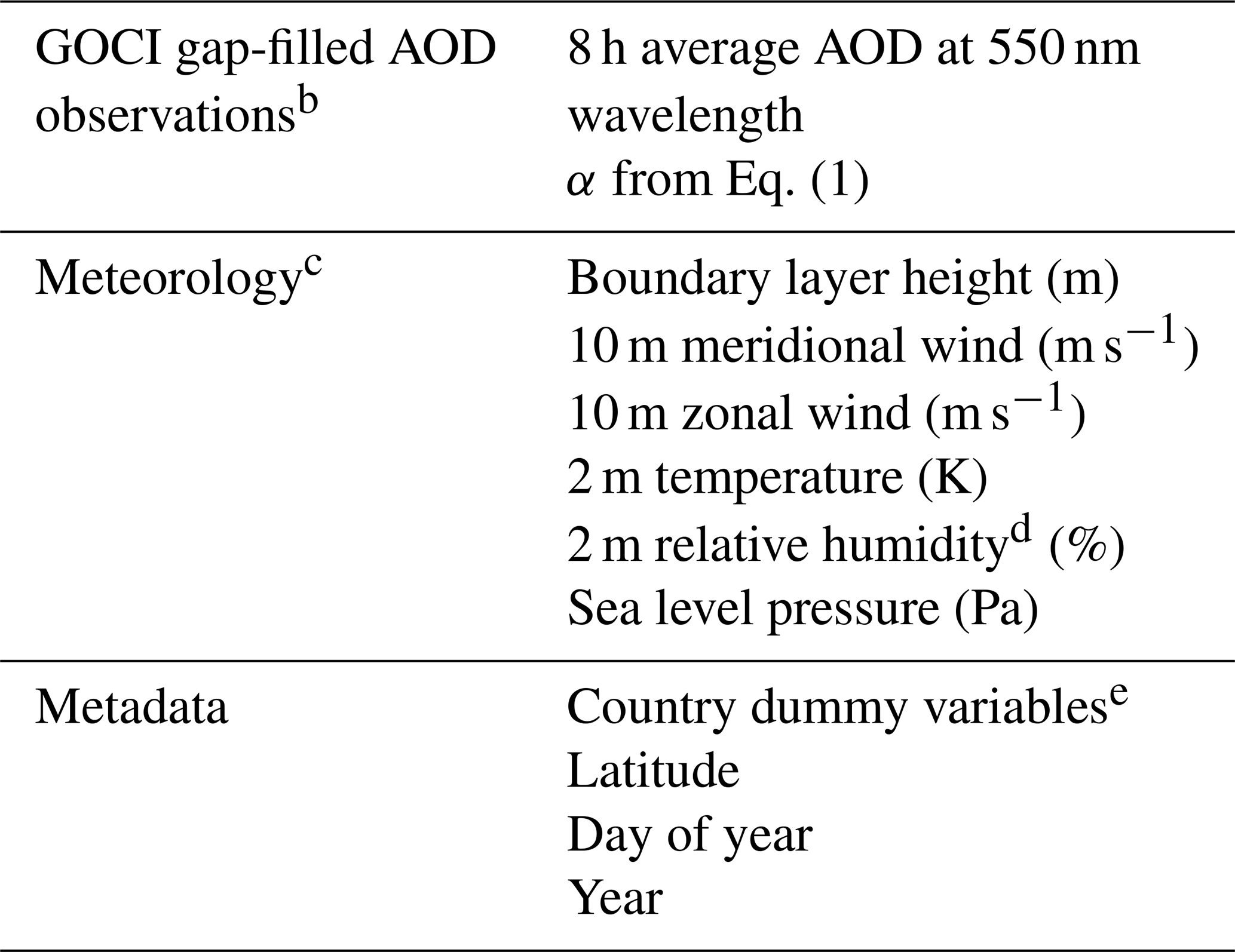
a The RF algorithm predicts continuous 24 h PM2.5 on a 6 × 6 km2 grid for eastern China, South Korea, and Japan after training with PM2.5 surface network data. b The 8 h average 550 nm AODs on the 6 × 6 km2 grid retrieved with the YAER V2 algorithm (Choi et al., 2018). c ECMWF ERA5 fields (Hersbach et al., 2020) at 30 × 30 km2 spatial resolution and hourly temporal resolution interpolated bilinearly to the GOCI grid and averaged over 24 h. d Estimated from temperature and dew point using the August–Roche–Magnus approximation (Alduchov and Eskridge, 1996). e The three variables that, for each of eastern China, South Korea, and Japan, have a value of 1 if a grid cell is within those national borders and of 0 otherwise.
Decision trees are fit recursively to the predictor variable. Suppose we have a collection of N data elements , denoted as xi, each composed of m predictor variables (xi∈Rm) and a corresponding list of N labels yi that we would like to learn. In our case, yi denotes the observed PM2.5 concentrations from the surface networks averaged on the 6 × 6 km2 grid, and N denotes the number of these observations. The algorithm works by splitting the data into left and right subsets, L and R, at an optimum split point determined from the predictor variables in xi (Pedregosa et al., 2011). The optimum split point is defined as the one that minimizes the impurity G, as follows:
where β represents the fraction of data in the subset L, and MSE represents the mean squared error of each of the subsets, as follows:
where is the mean of the target labels within a given subset X, and n is the number of elements in that subset. From there, the same algorithm is recursively applied to the left and right subsets L and R until the tree is grown. We follow the advice of Hastie et al. (2009) and grow trees until the data are fully classified (each leaf contains only one value).
Due to the recursive training structure, decision trees are sensitive to the data on which they are trained because a change in one split point changes the composition of all its child nodes. Individual decision trees thus have high error variance but no inherent bias. It follows that averaging many individual and uncorrelated trees should yield a low variance, low bias, prediction. We construct 200 trees in parallel and reduce the correlation between them through a bagging procedure; for each of the 200 decision trees in the RF, we sample the input data with replacement to form a new dataset of the same dimensions and then grow a decision tree from this bootstrapped data (Breiman, 2001). Because of the high input sensitivity, a wide variety of decorrelated trees are grown. The predictions of each individual tree are averaged to yield the prediction of the RF. We fit our RF using the RandomForestRegression class in the Python module Scikit-learn (Pedregosa et al., 2011). We attempted to further decorrelate the trees by following Breiman (2001) and calculating the split points of each individual tree using only a random subset of the m predictor variables; however, a sensitivity test we performed showed only minor differences with the base case, and therefore, we follow Geurts et al. (2006) in considering all predictor variables in the training process.
We evaluate how the RF generalizes to predictions for the full 6 × 6 km2 domain via a 10-fold cross-validation. For each fold of the cross-validation, we leave out a randomly selected 10 % of PM2.5 network sites (averaged on the 6 × 6 km2 grid if needed) from each country. These 10 % represent the test set. Because we perform the validation 10 times, each grid cell is in the test set exactly once. We compare the predicted PM2.5 to withheld observed PM2.5 using four metrics, i.e., root mean square error (RMSE), the RMSE divided by mean observed PM2.5 (relative RMSE or RRMSE), the coefficient of variation (R2), and the mean bias computed by averaging the difference between predicted and observed PM2.5 (MB).
An outcome of interest is the ability of our predictions to capture exceedances of National Ambient Air Quality Standards (NAAQS). We categorize each prediction within the test sets into one of the following four classes: true positives (TPs), where both predicted and observed PM2.5 exceed the NAAQS threshold, true negatives (TNs), where neither exceed the threshold, false positives (FPs), where an exceedance is predicted but not observed, and false negatives (FNs), where an exceedance is observed but not predicted (Brasseur and Jacob, 2017; Cusworth et al., 2018). We use these classes to compute three overall prediction grades. The first, percent of detection (POD), gives the fraction of observed exceedances that were successfully predicted, as follows:
The second, false alarm ratio (FAR), gives the fraction of predicted exceedances that did not occur as follows:
The third, equitable threat score (ETS), compares how well the prediction does relative to random chance, as follows:
where β is the number of true positives obtained by random chance, as follows:
ETS is 1 for perfect prediction skill and 0 for no better or worse than chance.
Predictor variable selection is an important task in implementing an RF, as the addition of non-informative variables can decrease performance. Unlike linear regression, which can naturally ignore unhelpful predictors, irrelevant data can, by chance, aid in minimizing impurity G at some stage in the optimization process, making all subsequent splits suboptimal. The six meteorological variables given in Table 1 are standard in the AOD PM2.5 prediction (e.g., Kloog et al., 2014; Li et al., 2017), while the four spatiotemporal variables (location dummies, latitude, year, and day of the year) and the retrieval gap-filling parameter α proved to be informative in sensitivity tests. In addition to the predictor variables in Table 1, we considered as additional variables the population density, the GOCI fine mode fraction (FMF), and the GOCI multiple prognostic expected error (MPEE), but we found that they worsened accuracy of the fit, and so we did not retain them. Because population density worsened the fit, we did not include other spatially varying but temporally fixed land use variables such as road data, elevation, or emissions. We also compared RFs trained on GOCI AOD and on GOCI–AHI-fused AOD and found no significant difference in the fitting of PM2.5. We, therefore, use the GOCI AOD product because of its longer record.
3.1 Accuracy and precision of RF predictions
Figure 3 shows scatterplots, color-coded by count, comparing surface observations of 24 h and annual mean PM2.5 to the predicted GOCI PM2.5 values in grid cells whose records are entirely withheld from training in the cross-validation procedure. GOCI PM2.5 values for the annual mean are obtained by averaging the 24 h predictions. Table 2 gives comprehensive GOCI PM2.5 evaluation statistics for East Asia and for each country. The 24 h predictions for East Asia have a negligible mean bias of 0.23 µg m−3 (annual; 0.22 µg m−3), though the RF underpredicts PM2.5 at the high tail of the distribution; we will return to that issue later in the context of NAAQS exceedances. The root mean square error (RMSE) between observed and predicted 24 h PM2.5 is 8.8 µg m−3 (annual; 3.3 µg m−3), corresponding to a relative RMSE (RRMSE) of 37 % (annual; 14 %), as defined in Sect. 2.3. The prediction captures 89 % of the observed 24 h variance (R2 = 0.89) and 96 % of annual variance (R2 = 0.96). These results compare favorably to previous reconstructions of PM2.5 from satellite AOD data. For example, a 1 km 2000–2015 continental USA product and 3 km 2015–2016 eastern China product have cross-validations R2 of 0.86 and 0.87, respectively, for daily PM2.5 (Di et al., 2019; Hu et al., 2019), while a global 0.01∘ 1998–2018 product and a 0.1∘ 2000–2016 product for China have cross-validated R2 of 0.90–0.92 and 0.77, respectively, for annual PM2.5 (Hammer et al., 2020; Xue et al., 2019). R2 for the annual mean PM2.5 in South Korea is relatively low (0.41), which can be explained by the weak dynamic range of observed annual PM2.5 in the country (Fig. 1), as will be discussed later in this section.
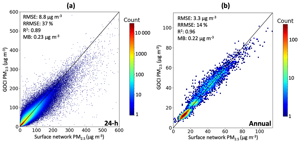
Figure 3The ability of the random forest algorithm to predict 24 h (a) and annual mean PM2.5 (b) in East Asia. Scatterplots depict the relationship between GOCI and surface network PM2.5 at grid cells withheld from training in the cross-validation. The plots are two-dimensional histograms, where the pixel color corresponds to the count of observation/prediction correspondences within the corresponding bin on a logged scale. The identity line is plotted in black. For the annual mean PM2.5, grid cells with fewer than 80 % of PM2.5 observation days in a given year are removed to avoid biasing the average values. For panel (a), 0.002 % of the data are not shown, as they exceed the plot range; all data are shown in panel (b).
Table 2Error statistics for fitting of PM2.5 data by the RF algorithm∗.
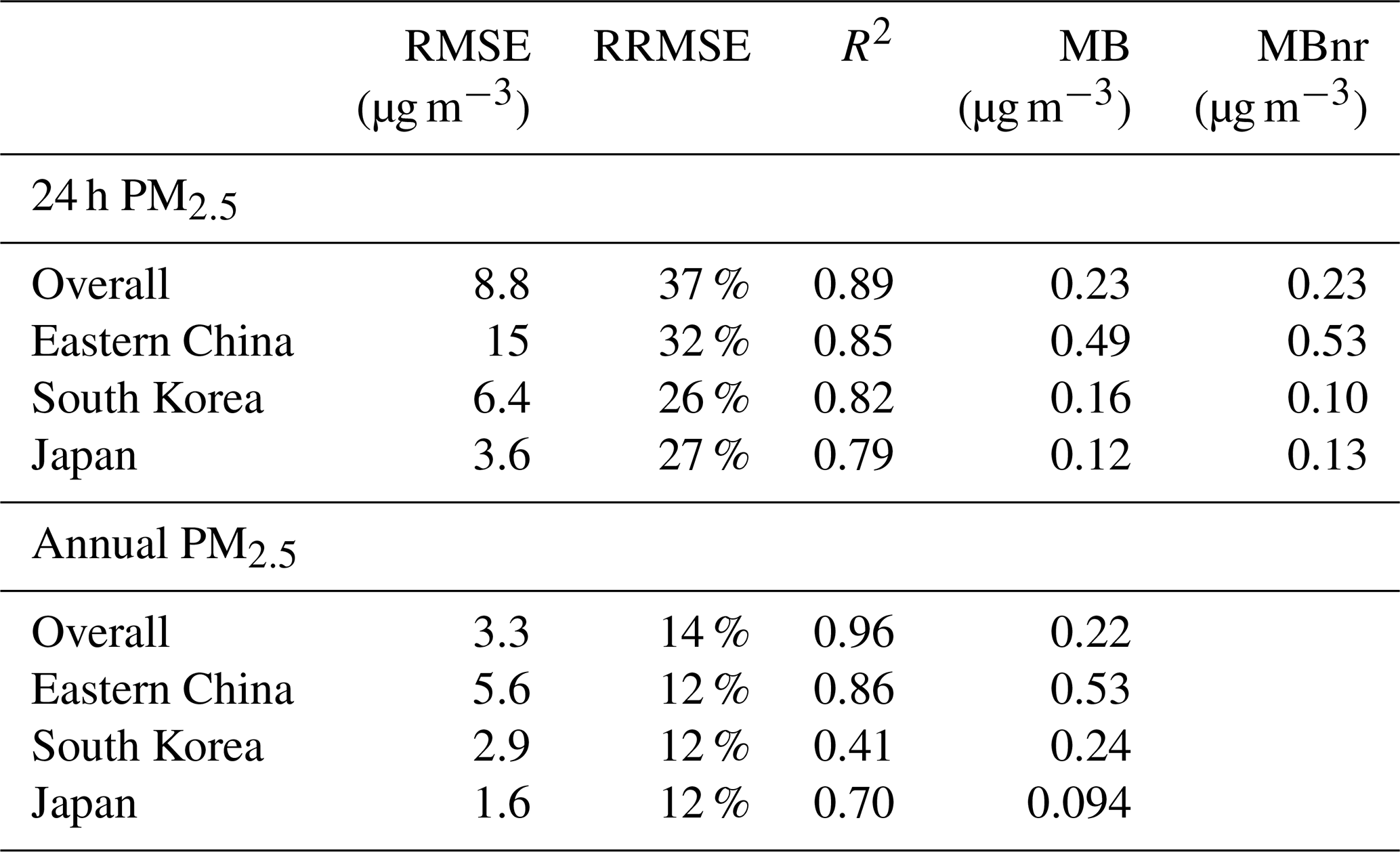
∗ Comparison statistics between GOCI and surface network PM2.5 for the grid cells in each of eastern China, South Korea, and Japan are completely withheld from the RF training process in the cross-validation procedure. Statistics shown are for the root mean square error (RMSE), relative RMSE (RRMSE), coefficient of variation (R2), mean bias (MB), and mean bias on days where AOD retrieval fails (MBnr).
Our gap-filling strategy does not introduce bias for days without GOCI observations (and with AOD inferred, instead, from Eq. 1). Figure S1 in the Supplement shows that surface network PM2.5 has distinct distributions on days where AOD retrieval fails compared to when AOD retrieval succeeds, a pattern successfully reproduced by GOCI PM2.5. Table 2 shows that the mean bias statistic on days where AOD retrieval fails is similar to the whole population. This suggests that the RF algorithm is able to successfully exploit the information encoded in AOD retrieval failure in making a PM2.5 prediction, a phenomenon also noted by Brokamp et al. (2018).
Table 3Ability of the RF algorithm to diagnose exceedances of air quality standardsa.
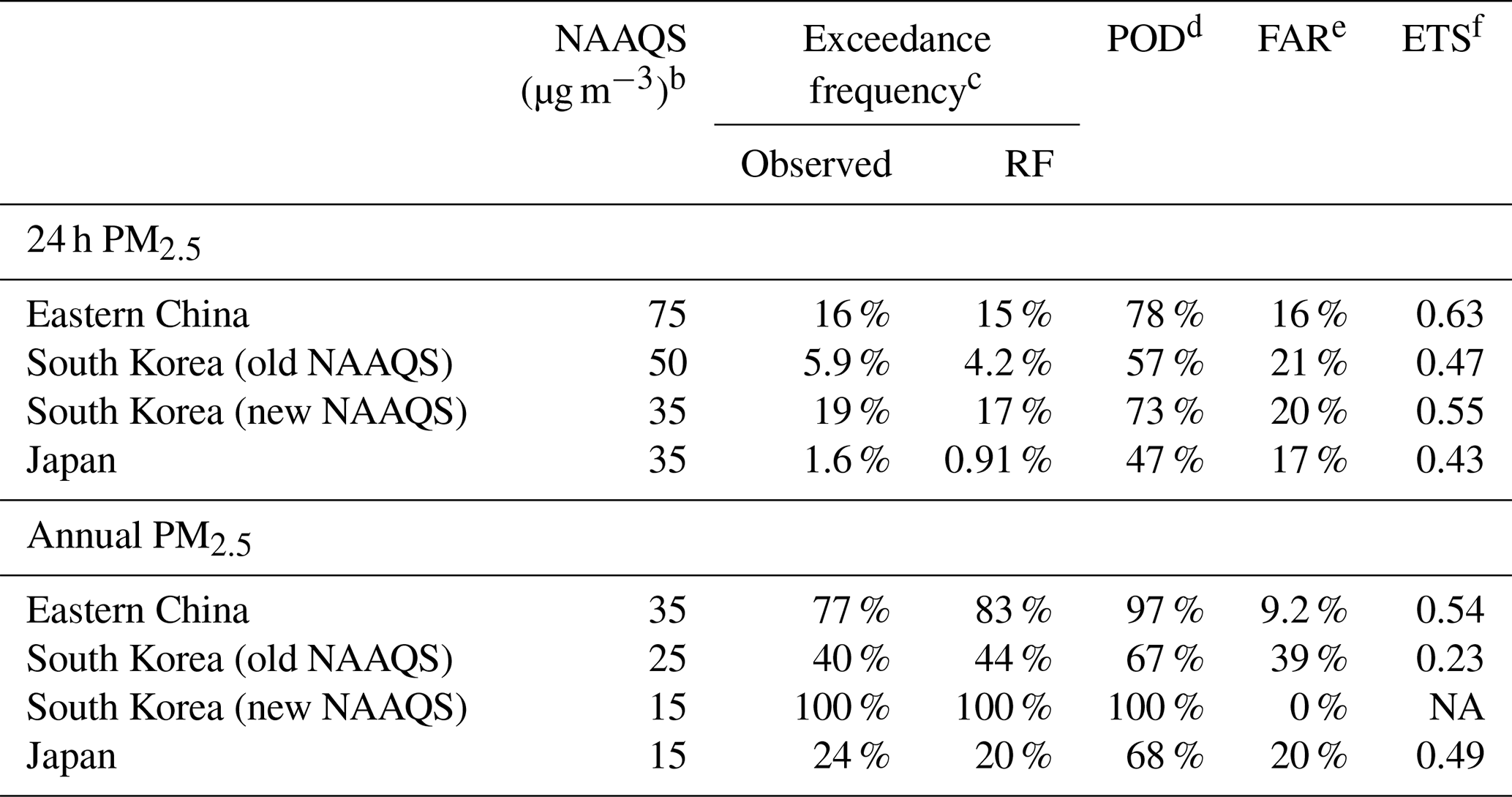
a Calculated using sites withheld from training in the cross-validation procedure. b National Ambient Air Quality Standards (NAAQS), which are specific to each country. We show results for the class 2 NAAQS in eastern China and for both pre-2018 (old) and post-2018 (new) NAAQS for South Korea because all observed grid cells exceed the new annual NAAQS of 15 µg m−3. c Percentage of site days (24 h standard) or site years (annual standard) exceeding the NAAQS. d Percent of detection (POD) defined as the percentage of exceedances successfully detected. e False alarm ratio (FAR) defined as the percentage of predicted exceedances that did not occur. f Equitable threat score (ETS), which is defined as the ability of the RF to predict exceedances beyond random chance.
One potential application of PM2.5 monitoring from space would be to diagnose exceedances of national ambient air quality standards (NAAQS) at locations without network sites. Table 3 shows the NAAQS for 24 h and annual PM2.5 for the three countries and the ability of GOCI PM2.5 to diagnose NAAQS exceedances in grid cells excluded from the training process in the cross-validation procedure. The 24 h exceedances correspond to the high tails of the distributions but annual exceedances are much more widespread. The POD column shows the percent of true positives successfully detected, while the FAR shows the rate of false positives (defined in Sect. 2.3). The POD for 24 h exceedances ranges from 47 %–78 % by country (16 %–21 % – FAR). PODs are higher for annual exceedances, but that reflects the higher observed frequency of these exceedances. The ETS values ranging from 0.43–0.63 indicate that the model captures exceedances with much better skill than random guessing.
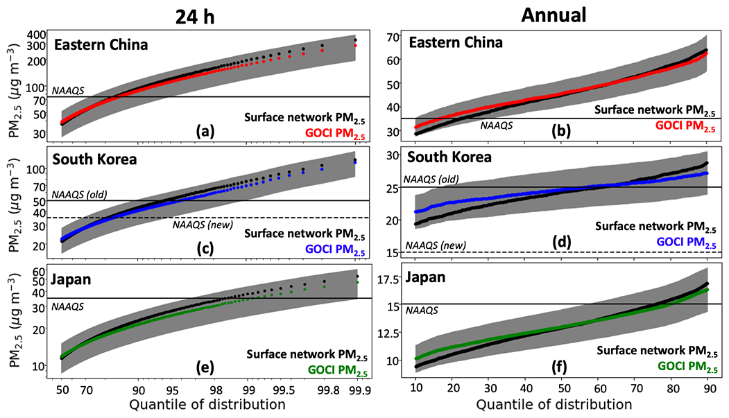
Figure 4Cumulative probability density functions (pdf's) of 24 h and annual mean PM2.5 concentrations in eastern China, South Korea, and Japan. Surface network PM2.5 (black) is compared to GOCI PM2.5 (colored) taken from the cross-validation. The gray envelope represents the relative root mean square error (RRMSE) of the RF algorithm, as given in Table 2, measuring the predictive capability of the algorithm for individual events. The NAAQS for each country is shown as the horizontal line, with both the pre-2018 and post-2018 NAAQS shown for South Korea. The left panel scales are log–log, while the right panel scales are linear, and the y-axis scales vary for the different countries.
The main difficulty for GOCI PM2.5 in predicting NAAQS exceedances is that many of those exceedances fall within the precision of individual predictions. This is illustrated in Fig. 4, with the cumulative probability density function (pdf) of the 24 h and annual mean PM2.5 concentrations in eastern China, South Korea, and Japan representing the same withheld data from the cross-validation as in Tables 2 and 3. The 24 h RRMSE of 26 %–32 %, depending on country (Table 2) is shown as the gray envelope and is relatively flat across the distribution. The prediction of NAAQS exceedances within that uncertainty envelope is limited by the precision of the algorithm. All of the 24 h exceedances in Japan are within that envelope, as are most of the exceedances in eastern China and Korea. China has the largest fraction of exceedances beyond the RRMSE of the GOCI PM2.5 and, therefore, the best prediction success. An additional, though smaller, cause of bias is that GOCI PM2.5 underestimates the high tail of the pdf, as is apparent in Fig. 4, which explains in particular why we achieve a better FAR than POD for 24 h PM2.5 in South Korea and Japan. Our worst NAAQS prediction performance is for annual PM2.5 in South Korea for the old 25 µg m−3 standard because most of the distribution is within the RRMSE envelope. Additionally, the already small dynamic range of the surface network annual PM2.5 (black dots) is underestimated by the GOCI PM2.5 (blue dots). These culminate in a GOCI PM2.5 estimate with good RMSE but low R2.
We experimented with several modifications to the RF algorithm to improve the prediction of NAAQS exceedances but with no success. These tests included training separate RFs for each of the three countries, training annual PM2.5 predictions on annual (rather than 24 h) PM2.5 data, directly predicting NAAQS exceedances by setting the learned label to be true if a day (year) is above the 24 h (annual) NAAQS for a given country, and applying different weights to the data so that the high tail is oversampled in the training process. None of these tests yielded significant improvements. Smoothing of the tails in RFs is a well-recognized problem (Zhang and Lu, 2012). Following Zhang and Lu (2012), we attempted to train RFs to predict and correct the residuals but found this to be ineffective. Part of this tail smoothing could also result from the underlying GOCI AOD land product, which has a negative bias (−0.02) for high AODs and a positive bias (+0.02) for low AODs (Choi et al., 2018).
3.2 PM2.5 temporal trends and spatial distributions
Figure 5 shows long-term trends of annual PM2.5 for each country, as measured by the PM2.5 surface network and as inferred in the GOCI PM2.5 for both areal- and population-weighted means. We do not include GOCI PM2.5 for years before the networks became available (and, hence, when the RF could be trained) because of concern over extrapolation bias. The PM2.5 networks show decreasing trends in all three countries, and these trends are consistent with the GOCI PM2.5 for both areal- and population-weighted means, demonstrating that the trends reported by the PM2.5 networks are representative of the countries. However, the PM2.5 networks in eastern China and South Korea underestimate the population-weighted means. Moreover, trends in South Korea and eastern China become flat between 2018 and 2019 (with a slight population-weighted increase in South Korea). This could possibly reflect interannual meteorological variability (Zhai et al., 2019; Koo et al., 2020) but also an increase in oxidants producing secondary aerosol (Huang et al., 2021). Figure S2 shows maps of annual GOCI PM2.5 across the entire study domain.
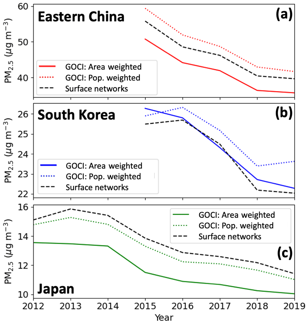
Figure 5Trends in the annual mean PM2.5 concentrations for eastern China, South Korea, and Japan. Trends determined from the national surface PM2.5 networks (dashed black line) averaged over 6 × 6 km2 grid cells, requiring at least 80 % of data for all years plotted, are compared to GOCI PM2.5 trends inferred by the random forest (RF) algorithm with continuous temporal and spatial coverage on the 6 × 6 km2 grid and weighted either by area (solid colored line) or by population (dashed colored line). Here we use an RF trained on all the data. The gridded population data are from CIESIN (2018). The national PM2.5 networks include 413 continuously observed grid cells in eastern China, 74 in South Korea, and 307 in Japan. Trends are initialized at the onset of the surface network for complete years of data; due to the unavailability of the early months of the year, 2011 is discarded for Japan, and 2014 is discarded for eastern China.
Figure 6 shows the changes in annual mean PM2.5 concentrations over South Korea between 2015 and 2019 as observed from the national network and as inferred from GOCI. We focus on South Korea here because it demonstrates how GOCI PM2.5 adds considerable information to a region that already has relatively good network coverage, including the detection of PM2.5 hot spots missing from the network, such as the Iksan region on the west coast of South Korea in 2015 that was subsequently added to the network by 2019. Figures S3 and S4 show analogous maps for China and Japan, respectively.
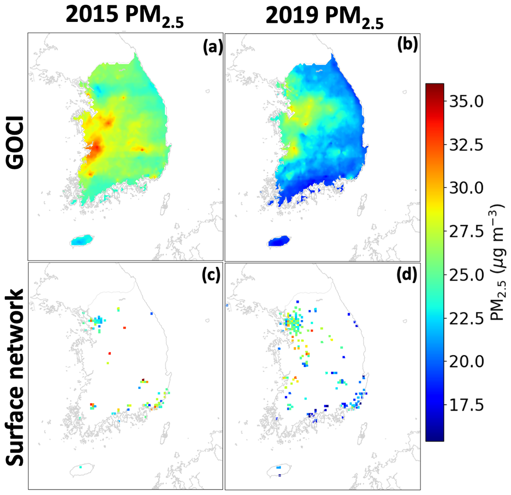
Figure 6Annual mean PM2.5 concentrations in South Korea in 2015 and 2019. GOCI PM2.5 (a, b) inferred from an RF trained on all available data are compared to AirKorea network observations (c, d). Network observations are shown only if at least 80 % of the year was observed.
Figure 7 depicts the relative 2015–2019 trends of PM2.5 concentrations in South Korea derived from a linear regression applied to the annual GOCI PM2.5 in each 6 × 6 km2 grid cell. Such a spatially resolved trend analysis is uniquely enabled by the GOCI coverage. We find decreases across the country, except in the Seoul metropolitan area, which mostly shows no significant trend except for a few pixels in Incheon. These results are consistent with the spatial patterns calculated from AirKorea data by Yeo and Kim (2019), who found 2015–2018 decreases in Incheon but not Seoul or the surrounding Gyeonggi province. Despite the insignificant changes in Seoul, substantial PM2.5 decreases are found over other large urban areas including Busan, Ulsan, Daegu, and Gwangju. The three rapidly decreasing spots on the southern coast are Gwangyang, Sacheon, and Changwon, which house industrial complexes related to the South Korean shipbuilding industry that has recently declined (Jung-a, 2016). Figure S5 shows absolute 2015–2019 trends of GOCI PM2.5 concentrations across the entire study domain and demonstrates that the North China Plain has the largest overall PM2.5 reductions.
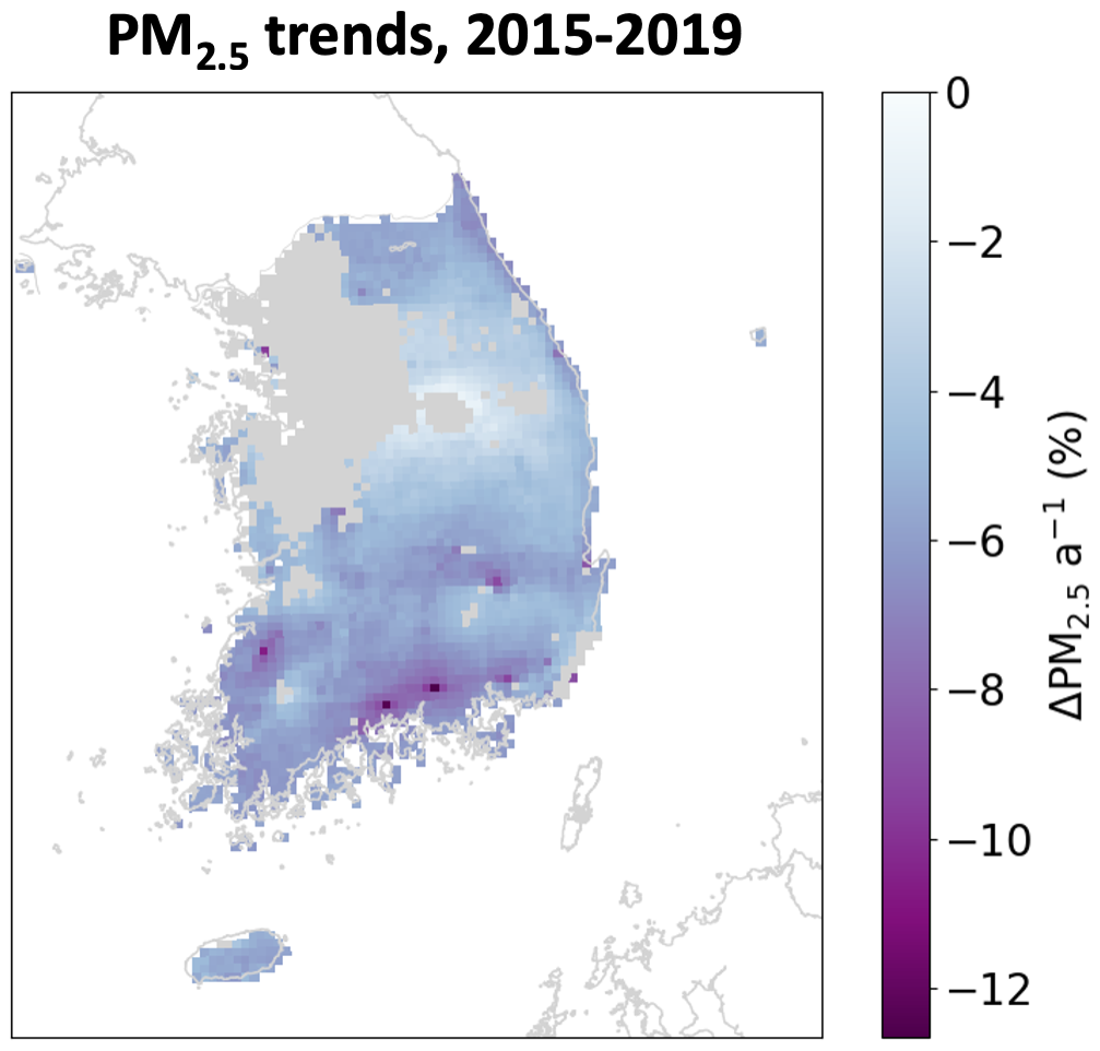
Figure 7The 2015–2019 trends per year in PM2.5 concentrations across South Korea. The trends are obtained by ordinary linear regression of the annual mean GOCI PM2.5 in each 6 × 6 km2 grid cell, with significant regression slopes (p<0.05) where the RF is trained on all the available data. Grid cells with insignificant trends are plotted in gray.
AOD and PM2.5 in East Asia tend to have opposite seasonalities driven by boundary layer depth and RH (Zhai et al., 2021). Figure 8 compares GOCI and the surface network monthly mean PM2.5 in the Beijing, Seoul, and Tokyo metropolitan areas, with predictions coming from withheld data in the 10-fold cross-validation. Correspondence between GOCI and the network PM2.5 may be tighter than the nationwide annual means plotted in Fig. 5 because these urban areas are well observed. We see that the RF algorithm fully captures the observed seasonality in PM2.5, although some observed monthly spikes are underestimated. The figure illustrates the lack of trend in the Seoul metropolitan area over 2015–2019 but also shows that winter and summer PM2.5 in the region have opposite and roughly equal trends, with winter growing more polluted while summers become cleaner.
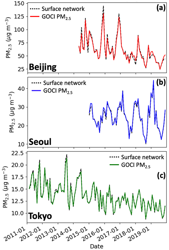
Figure 8Monthly PM2.5 concentrations in the Beijing, Seoul, and Tokyo metropolitan areas. GOCI PM2.5 inferred from the RF algorithm for totally withheld sites in the cross-validation are compared to network observations. Beijing is defined by the namesake's province boundary, Seoul by the Seoul and Incheon boundaries, and Tokyo is defined as the Ibaraki, Saitama, Chiba, Tokyo, Kanagawa, and Yamanashi prefectures.
3.3 Urban-scale pollution events
We examine here the ability of GOCI PM2.5 to capture the spatial and temporal variability of PM2.5 pollution events on urban scales. Figure 9 shows a map of GOCI PM2.5 – produced by a RF trained on all the data, with the surface network PM2.5 overlaid – across the Seoul metropolitan area on 24–29 May 2016, corresponding to a severe pollution event sampled during the Korea–United States Air Quality (KORUS-AQ) field campaign (Crawford et al., 2021). The dense PM2.5 network for Seoul shows large variability at the sub-6 × 6 km2 scale that GOCI does not resolve. However, GOCI PM2.5 captures most of the variability in the network data aggregated on the 6 × 6 km2 grid (R2=0.74). It also successfully captures the day-to-day variability during the event.
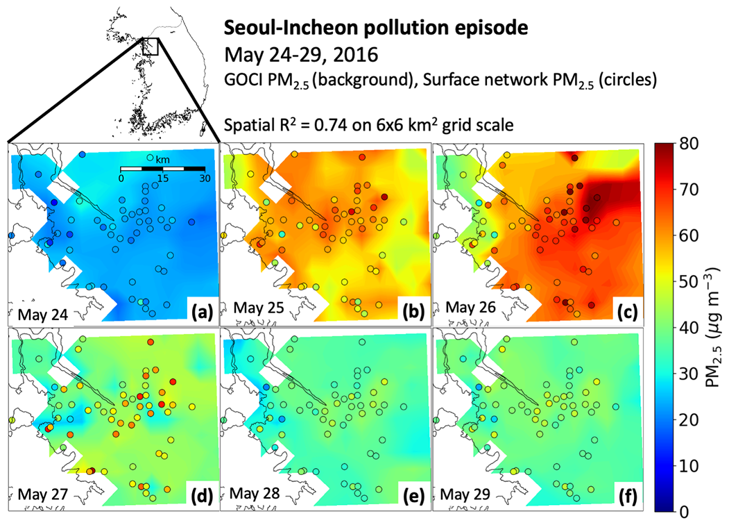
Figure 9The 24 h PM2.5 concentrations during a pollution event in Seoul–Incheon (24–29 May 2016). GOCI PM2.5 inferred from the RF algorithm (background; 6 × 6 km2 grid scale) trained on all available data is compared to observations from the AirKorea surface network (circles).
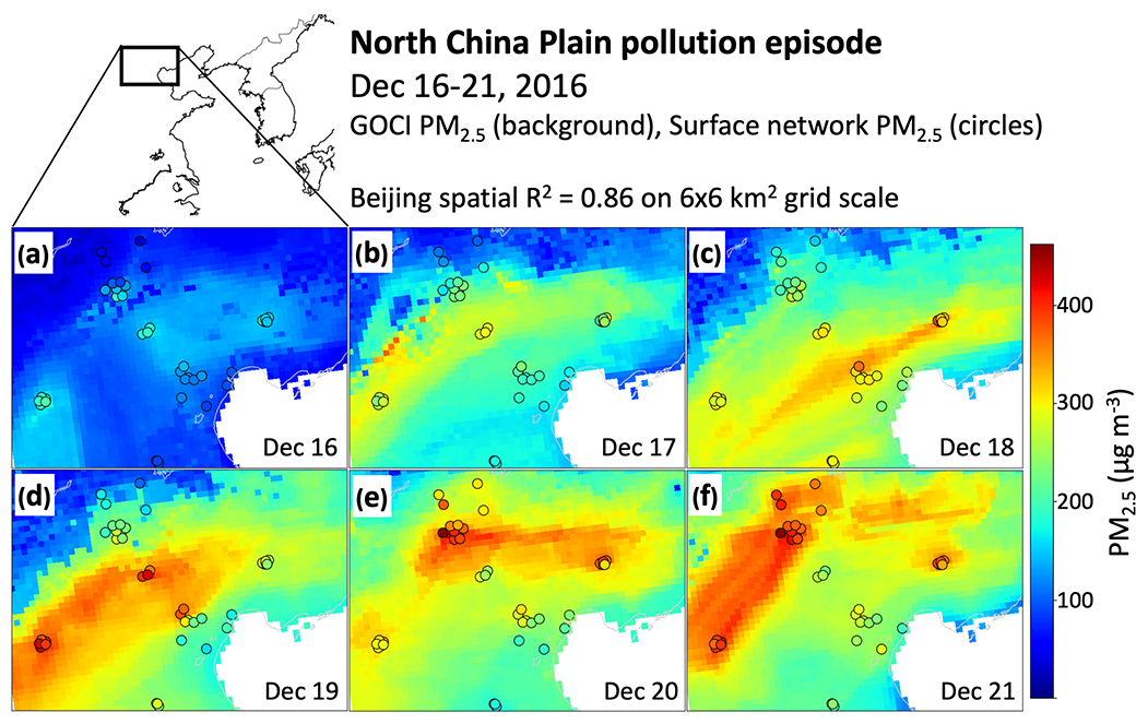
Figure 10Same as Fig. 9 but for a pollution event in Beijing on 16–21 December 2016.
Figure 10 shows an additional test of the RF algorithm with one of the most severe pollution events in the record, the 16–21 December 2016 Beijing winter haze episode. The 24 h PM2.5 concentrations exceeded 400 µg m−3 at some of the network sites. While there is a tight correspondence between the GOCI and surface network 24 h PM2.5 for Beijing grid cells (R2 range of 0.74–0.99), the network observations are on average 20 µg m−3 higher than the GOCI PM2.5. The difference is most pronounced at the December 21 concentration peak which has mean observed value 396 µg m−3 to the predicted 348 µg m−3. This reflects the RF smoothing and AOD underestimate for the high tail of the distribution, as previously illustrated in Fig. 4. It nevertheless illustrates the ability of GOCI, combined with our gap-filling method, to capture severe winter haze episodes that are particularly challenging to observe from space.
3.4 Regional air quality model evaluation
Regional air quality model predictions of PM2.5 are typically evaluated with observations from surface network sites, but the spatially continuous GOCI PM2.5 fields offer more extensive coverage and, hence, a broader opportunity for model evaluation. We demonstrate this capability here with the Community Multiscale Air Quality Modeling System (CMAQ, version 4.7.1) simulations for the Korean peninsula including both South and North Korea at 9 km resolution (Bae et al., 2018, 2021). There are no surface PM2.5 data in North Korea to train the RF, so we use the South Korea categorical variable to generate the GOCI PM2.5 fields there.
The simulation for South Korea was conducted for 2015–2019 using emissions from the Clean Air Policy Support System (CAPSS) 2016 (Choi et al., 2020) for South Korea and KORUSv5 (Woo et al., 2022) for outside South Korea. The simulation for North Korea was conducted for 2016 using emissions from the Comprehensive Regional Emissions inventory for Atmospheric Transport Experiment (CREATE) 2015 (Woo et al., 2020) and CAPSS 2013. Natural aerosols, including sea salt and mineral dust, are included. To prepare the boundary conditions, a coarse domain at 27 km horizontal grid resolution covering northeastern Asia was used.
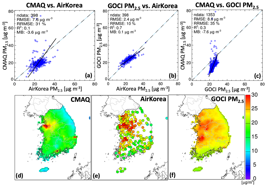
Figure 11Mean PM2.5 concentrations in South Korea in 2015–2019 as simulated by CMAQ, measured at the AirKorea sites, and inferred from GOCI. Panels (a), (b), and (c) show scatterplots comparing the CMAQ and GOCI PM2.5 fields to the AirKorea measurements (398 sites) and CMAQ to GOCI PM2.5 on the 9 × 9 km2 CMAQ grid (1353 grid cells to compare). Panels (d), (e), and (f) show maps of the mean 2015–2019 concentrations.
Figure 11 illustrates the increased capability for model evaluation in South Korea enabled by the GOCI PM2.5 fields. The bottom row shows the mean 2015–2019 PM2.5 concentrations in CMAQ compared to the AirKorea network and to GOCI PM2.5, and the top row shows comparison scatterplots. The top left panel compares the CMAQ simulation to 2015–2019 mean PM2.5 observations from the 398 AirKorea network sites. The top middle panel compares the GOCI PM2.5 to the same AirKorea network data, showing excellent agreement. The GOCI PM2.5 fields provide 1353 points for South Korea on the 9 × 9 km2 CMAQ grid, and the top right panel shows the resulting increase in capability for evaluation of the CMAQ simulation. It shows, in particular, that CMAQ underestimates PM2.5 in coastal environments, possibly because of unaccounted ship emissions.

Figure 12Mean PM2.5 concentrations in North Korea in 2016, as simulated by CMAQ and as represented by the GOCI PM2.5 product, assuming that South Korea is a categorical variable. Panel (b) shows surface PM2.5 concentrations from the AirKorea and China Ministry of Ecology and Environment (MEE) networks.
Figure 12 evaluates the CMAQ simulation with the GOCI PM2.5 fields over North Korea. Unlike in South Korea, there are no observation sites in North Korea and GOCI PM2.5 offers the only opportunity for local evaluation. CMAQ and GOCI PM2.5 show dramatically different patterns. The highest PM2.5 in CMAQ is in the Pyongyang capital region, while GOCI shows highest values in the north–central region. The lack of reliable emission inventories for North Korea makes it difficult to arbitrate this difference. The RF is not trained for North Korea, which might lead to positive biases because the AOD PM2.5 ratio modeled in the Zhai et al. (2021) GEOS-Chem simulation is higher over North Korea outside the mountainous east (range of 0.010–0.013 m3 µg−1) than over South Korea (0.008–0.010 m3 µg−1). However, the difference could also be explained by missing emissions in the inventory. Further evaluation could be done with border sites in South Korea and northeastern China. China Ministry of Ecology and Environment (MEE) sites along the border are consistent with high PM2.5 in north–central North Korea.
We used 2011–2019 geostationary aerosol optical depth (AOD) observations from the GOCI satellite instrument, in combination with a random forest (RF) machine learning algorithm trained on air quality network data, to produce a continuous 24 h PM2.5 data set for eastern China, South Korea, and Japan at 6 × 6 km2 resolution. The resulting gap-free GOCI PM2.5 product complements the air quality networks that cover only 1 % of 6 × 6 km2 grid cells in eastern China, 7 % in South Korea, and 8 % in Japan. It provides a general dataset for PM2.5 mapping to serve regional pollution analysis, air quality monitoring, and public health applications.
We trained the RF algorithm on gap-filled AODs from the GOCI instrument and a suite of 12 meteorological, geographical, and temporal predictor variables. Gap-filling of AODs was done by a weighted combination of nearest-neighbor data and chemical transport model fields, with the weight serving as an additional predictor variable. The RF algorithm is successfully able to exploit information encoded in AOD retrieval failure to produce a continuous product. Testing of the RF algorithm by the prediction of withheld network sites shows single-value precisions in each country of 26 %–32 % for 24 h PM2.5 and 12 % for annual mean PM2.5, with negligible mean bias. Accuracy statistics for PM2.5 inferred on grid cells with no AOD retrieval (i.e., estimated using Eq. 1) show similar accuracy statistics to that of the entire population, indicating that the gap-filling procedure does not bias the results. The algorithm has only moderate success at predicting NAAQS exceedance events because most of these events are within the single-value precision and also because of some smoothing of the extreme high tail of the PM2.5 frequency distribution.
We compared the continuous 24 h GOCI PM2.5 fields to spatial and temporal patterns observed at the national network sites. National trends of PM2.5 inferred from GOCI and weighted by area or population are consistent with those observed at network sites (2015–2019 in eastern China and South Korea; 2011–2019 in Japan), confirming that the trends observed at these sites are representative. However, the network sites in eastern China and South Korea underestimate population exposure. The GOCI PM2.5 fields over South Korea show PM2.5 hot spots missing in the early AirKorea network (2015) that are confirmed by subsequent addition of sites to the network (2019). The spatial distribution of GOCI PM2.5 trends in South Korea shows decreases everywhere, except in the Seoul metropolitan area where trends are flat. We show with the time series in the capital cities (Beijing, Seoul, and Tokyo) that the RF successfully captures the seasonality of PM2.5 even though AOD and PM2.5 have different and often opposite seasonalities.
We examined the ability of the RF algorithm to map air quality on urban scales by an analysis of two multi-day pollution episodes in Seoul and Beijing. The algorithm captures the day-to-day temporal variability observed by the surface networks and the spatial variability on the 6 × 6 km2 scale. The highest PM2.5 concentrations are underpredicted, which reflects the smoothing of the high tail of the distribution.
The continuous spatial coverage of PM2.5 provided by the GOCI fields enables improved evaluation of the air quality models used in support of emission control policies. A comparison to a CMAQ simulation for South Korea in 2015–2019 reveals a large model underestimate in coastal environments undersampled by the AirKorea network. A comparison to a CMAQ simulation for North Korea in 2016, where the RF provides the only PM2.5 data for model evaluation, shows drastically different patterns, with the RF featuring high PM2.5 throughout North Korea. The RF results in North Korea could be affected by errors due to lack of training data but they appear consistent with the PM2.5 network observations at Chinese border sites.
More work could be done to improve our GOCI PM2.5 product. We find, in our current RF algorithm, consistent with Hu et al. (2017), that the addition of certain predictor variables such as population decreases performance. This motivated our practice of excluding spatially varying but temporally constant fields such as elevation and emissions. However, these variables have been found to be useful in other inferences of PM2.5 from AOD data (Kloog et al., 2012; Di et al., 2019), so further investigation is needed on how to accommodate them in our modeling framework. A higher-resolution meteorological reanalysis, such as ERA5-Land (Muñoz-Sabater et al., 2021), could be used for the meteorological predictor variables and enable the inclusion of additional variables such as precipitation. Additional remote sensing products such as Normalized Difference Vegetation Index (NDVI) could also be useful. More work needs to be done to address our underestimate of the high tail of the PM2.5 distribution, i.e., extreme pollution events. Such an underestimate is common in RF applications (Zhang and Lu, 2012) but could be addressed by leveraging specialized statistical tools like extreme value theory. Additional training methods could be used to improve the ability of the RF to predict NAAQS exceedances, such as data sampling adjustments. Moreover, it is possible that skill in modeling NAAQS exceedance could be improved by leveraging data that better capture diurnal variations of PM2.5, as high concentrations tend to occur at night. The unique geostationary capability of GOCI to generate hourly AOD data could be used to produce an hourly PM2.5 product. A new GOCI AOD product with 2 × 2 km2 resolution is expected to become available in the near future and will provide the motivation to explore these improvements in a new version of our RF algorithm.
The 24 h 6 × 6 km2 resolution daily GOCI PM2.5 data are made freely available on Dataverse at https://doi.org/10.7910/DVN/0L3IP7 (Pendergrass et al., 2021).
The supplement related to this article is available online at: https://doi.org/10.5194/amt-15-1075-2022-supplement.
DCP and DJJ designed the study. DCP developed the RF and performed analysis. SZ, MB, and SK ran and analyzed the chemical transport model data. SL aided in satellite data processing. JK, HL, and JHK provided the scientific interpretation and discussion. All authors provided input on the paper for revision.
The contact author has declared that neither they nor their co-authors have any competing interests.
Publisher’s note: Copernicus Publications remains neutral with regard to jurisdictional claims in published maps and institutional affiliations.
This work was funded by the Samsung PM2.5 Strategic Research Program and the Harvard-NUIST Joint Laboratory for Air Quality and Climate (JLAQC). GOCI data were provided by the Korea Institute of Ocean Science and Technology (KIOST). Drew C. Pendergrass was funded by U.S. National Science Foundation Graduate Fellowships Program. We thank the two anonymous reviewers for their thoughtful feedback.
This research has been supported by the Samsung Advanced Institute of Technology (Samsung PM2.5 Strategic Research Program), the Harvard-NUIST Joint Laboratory for Air Quality and Climate (JLAQC), and the U.S. National Science Foundation Graduate Fellowships Program.
This paper was edited by Marloes Penning de Vries and reviewed by two anonymous referees.
Alduchov, O. A. and Eskridge, R. E.: Improved Magnus Form Approximation of Saturation Vapor Pressure, J. Appl. Meteor., 35, 601–609, https://doi.org/10.1175/1520-0450(1996)035<0601:IMFAOS>2.0.CO;2, 1996.
Bae, M., Kim, H. C., Kim, B.-U., and Kim, S.: PM2.5 Simulations for the Seoul Metropolitan Area: (V) Estimation of North Korean Emission Contribution, J. Korean Soc. Atmos. Environ., 34, 294–305, https://doi.org/10.5572/KOSAE.2018.34.2.294, 2018.
Bae, M., Kim, B.-U., Kim, H. C., Kim, J., and Kim, S.: Role of emissions and meteorology in the recent PM2.5 changes in China and South Korea from 2015 to 2018, Environ. Pollut., 270, 116233, https://doi.org/10.1016/j.envpol.2020.116233, 2021.
Brasseur, G. P. and Jacob, D. J: Modeling of Atmospheric Chemistry, Cambridge University Press, Cambridge, UK, https://doi.org/10.1017/9781316544754, 2017.
Breiman, L.: Random Forests, Mach. Learn., 45, 5–32, https://doi.org/10.1023/A:1010933404324, 2001.
Brokamp, C., Jandarov, R., Hossain, M., and Ryan, P.: Predicting Daily Urban Fine Particulate Matter Concentrations Using a Random Forest Model, Environ. Sci. Technol., 52, 4173–4179, https://doi.org/10.1021/acs.est.7b05381, 2018.
Burnett, R., Chen, H., Szyszkowicz, M., Fann, N., Hubbell, B., Pope, C. A., Apte, J. S., Brauer, M., Cohen, A., Weichenthal, S., Coggins, J., Di, Q., Brunekreef, B., Frostad, J., Lim, S. S., Kan, H., Walker, K. D., Thurston, G. D., Hayes, R. B., Lim, C. C., Turner, M. C., Jerrett, M., Krewski, D., Gapstur, S. M., Diver, W. R., Ostro, B., Goldberg, D., Crouse, D. L., Martin, R. V., Peters, P., Pinault, L., Tjepkema, M., Donkelaar, A. van, Villeneuve, P. J., Miller, A. B., Yin, P., Zhou, M., Wang, L., Janssen, N. A. H., Marra, M., Atkinson, R. W., Tsang, H., Thach, T. Q., Cannon, J. B., Allen, R. T., Hart, J. E., Laden, F., Cesaroni, G., Forastiere, F., Weinmayr, G., Jaensch, A., Nagel, G., Concin, H., and Spadaro, J. V.: Global estimates of mortality associated with long-term exposure to outdoor fine particulate matter, P. Natl. Acad. Sci. USA, 115, 9592–9597, https://doi.org/10.1073/pnas.1803222115, 2018.
Center for International Earth Science Information Network – CIESIN – Columbia University: Gridded Population of the World, Version 4 (GPWv4): Population Density, Revision 11, NASA Socioeconomic Data and Applications Center (SEDAC) [dataset], https://doi.org/10.7927/H49C6VHW, 2018.
Chen, J., Yin, J., Zang, L., Zhang, T., and Zhao, M.: Stacking machine learning model for estimating hourly PM2.5 in China based on Himawari 8 aerosol optical depth data, Sci. Total Environ., 697, 134021, https://doi.org/10.1016/j.scitotenv.2019.134021, 2019.
Choi, J.-K., Park, Y. J., Ahn, J. H., Lim, H.-S., Eom, J., and Ryu, J.-H.: GOCI, the world's first geostationary ocean color observation satellite, for the monitoring of temporal variability in coastal water turbidity, J. Geophys. Res.-Oceans, 117, C09004, https://doi.org/10.1029/2012JC008046, 2012.
Choi, M., Kim, J., Lee, J., Kim, M., Park, Y.-J., Jeong, U., Kim, W., Hong, H., Holben, B., Eck, T. F., Song, C. H., Lim, J.-H., and Song, C.-K.: GOCI Yonsei Aerosol Retrieval (YAER) algorithm and validation during the DRAGON-NE Asia 2012 campaign, Atmos. Meas. Tech., 9, 1377–1398, https://doi.org/10.5194/amt-9-1377-2016, 2016.
Choi, M., Kim, J., Lee, J., Kim, M., Park, Y.-J., Holben, B., Eck, T. F., Li, Z., and Song, C. H.: GOCI Yonsei aerosol retrieval version 2 products: an improved algorithm and error analysis with uncertainty estimation from 5-year validation over East Asia, Atmos. Meas. Tech., 11, 385–408, https://doi.org/10.5194/amt-11-385-2018, 2018.
Choi, S., Kim, T., Lee, H., Kim, H., Han, J., Lee, K., Lim, E., Shin, S., Jin, H., Cho, E., Kim, Y., and Yoo, C.: Analysis of the National Air Pollutant Emission Inventory (CAPSS 2016) and the Major Cause of Change in Republic of Korea, Asian J. Atmos. Environ, 14, 422–445, https://doi.org/10.5572/ajae.2020.14.4.422, 2020.
Crawford, J. H., Ahn, J.-Y., Al-Saadi, J., Chang, L., Emmons, L. K., Kim, J., Lee, G., Park, J.-H., Park, R. J., Woo, J. H., Song, C.-K., Hong, J.-H., Hong, Y.-D., Lefer, B. L., Lee, M., Lee, T., Kim, S., Min, K.-E., Yum, S. S., Shin, H. J., Kim, Y.-W., Choi, J.-S., Park, J.-S., Szykman, J. J., Long, R. W., Jordan, C. E., Simpson, I. J., Fried, A., Dibb, J. E., Cho, S., and Kim, Y. P.: The Korea–United States Air Quality (KORUS-AQ) field study, Elementa: Science of the Anthropocene, 9, 00163, https://doi.org/10.1525/elementa.2020.00163, 2021.
Cusworth, D. H., Jacob, D. J., Sheng, J.-X., Benmergui, J., Turner, A. J., Brandman, J., White, L., and Randles, C. A.: Detecting high-emitting methane sources in oil/gas fields using satellite observations, Atmos. Chem. Phys., 18, 16885–16896, https://doi.org/10.5194/acp-18-16885-2018, 2018.
Di, Q., Amini, H., Shi, L., Kloog, I., Silvern, R., Kelly, J., Sabath, M. B., Choirat, C., Koutrakis, P., Lyapustin, A., Wang, Y., Mickley, L. J., and Schwartz, J.: An ensemble-based model of PM2.5 concentration across the contiguous United States with high spatiotemporal resolution, Environ. Int., 130, 104909, https://doi.org/10.1016/j.envint.2019.104909, 2019.
Dominici, F., Peng, R. D., Bell, M. L., Pham, L., McDermott, A., Zeger, S. L., and Samet, J. M.: Fine particulate air pollution and hospital admission for cardiovascular and respiratory diseases, Journal of the American Medical Association, 295, 1127–1134, https://doi.org/10.1001/jama.295.10.1127, 2006.
Gaspari, G. and Cohn, S. E.: Construction of correlation functions in two and three dimensions, Q. J. Roy. Meteor. Soc., 125, 723–757, https://doi.org/10.1002/qj.49712555417, 1999.
Geng, G., Zhang, Q., Martin, R. V., van Donkelaar, A., Huo, H., Che, H., Lin, J., and He, K.: Estimating long-term PM2.5 concentrations in China using satellite-based aerosol optical depth and a chemical transport model, Remote Sens. Environ., 166, 262–270, https://doi.org/10.1016/j.rse.2015.05.016, 2015.
Geng, G., Meng, X., He, K., and Liu, Y.: Random forest models for PM2.5 speciation concentrations using MISR fractional AODs, Environ. Res. Lett., 15, 034056, https://doi.org/10.1088/1748-9326/ab76df, 2020.
Geurts, P., Ernst, D., and Wehenkel, L.: Extremely randomized trees, Mach. Learn., 63, 3–42, https://doi.org/10.1007/s10994-006-6226-1, 2006.
Guo, B., Zhang, D., Pei, L., Su, Y., Wang, X., Bian, Y., Zhang, D., Yao, W., Zhou, Z., and Guo, L.: Estimating PM2.5 concentrations via random forest method using satellite, auxiliary, and ground-level station dataset at multiple temporal scales across China in 2017, Sci. Total Environ., 778, 146288, https://doi.org/10.1016/j.scitotenv.2021.146288, 2021.
Gupta, P. and Christopher, S. A.: Particulate matter air quality assessment using integrated surface, satellite, and meteorological products: Multiple regression approach, J. Geophys. Res.-Atmos., 114, D14205, https://doi.org/10.1029/2008JD011496, 2009.
Hammer, M. S., van Donkelaar, A., Li, C., Lyapustin, A., Sayer, A. M., Hsu, N. C., Levy, R. C., Garay, M. J., Kalashnikova, O. V., Kahn, R. A., Brauer, M., Apte, J. S., Henze, D. K., Zhang, L., Zhang, Q., Ford, B., Pierce, J. R., and Martin, R. V.: Global Estimates and Long-Term Trends of Fine Particulate Matter Concentrations (1998–2018), Environ. Sci. Technol., 54, 7879–7890, https://doi.org/10.1021/acs.est.0c01764, 2020.
Hastie, T., Tibshirani, R., and Friedman, J.: Random Forests, in: The Elements of Statistical Learning: Data Mining, Inference, and Prediction, edited by: Hastie, T., Tibshirani, R., and Friedman, J., Springer, New York, NY, 587–604, https://doi.org/10.1007/978-0-387-84858-7_15, 2009.
Hersbach, H., Bell, B., Berrisford, P., Hirahara, S., Horányi, A., Muñoz-Sabater, J., Nicolas, J., Peubey, C., Radu, R., Schepers, D., Simmons, A., Soci, C., Abdalla, S., Abellan, X., Balsamo, G., Bechtold, P., Biavati, G., Bidlot, J., Bonavita, M., Chiara, G. D., Dahlgren, P., Dee, D., Diamantakis, M., Dragani, R., Flemming, J., Forbes, R., Fuentes, M., Geer, A., Haimberger, L., Healy, S., Hogan, R. J., Hólm, E., Janisková, M., Keeley, S., Laloyaux, P., Lopez, P., Lupu, C., Radnoti, G., Rosnay, P. de, Rozum, I., Vamborg, F., Villaume, S., and Thépaut, J.-N.: The ERA5 global reanalysis, Q. J. Roy. Meteor. Soc., 146, 1999–2049, https://doi.org/10.1002/qj.3803, 2020.
Hu, H., Hu, Z., Zhong, K., Xu, J., Zhang, F., Zhao, Y., and Wu, P.: Satellite-based high-resolution mapping of ground-level PM2.5 concentrations over East China using a spatiotemporal regression kriging model, Sci. Total Environ., 672, 479–490, https://doi.org/10.1016/j.scitotenv.2019.03.480, 2019.
Hu, X., Belle, J. H., Meng, X., Wildani, A., Waller, L. A., Strickland, M. J., and Liu, Y.: Estimating PM2.5 Concentrations in the Conterminous United States Using the Random Forest Approach, Environ. Sci. Technol., 51, 6936–6944, https://doi.org/10.1021/acs.est.7b01210, 2017.
Huang, K., Xiao, Q., Meng, X., Geng, G., Wang, Y., Lyapustin, A., Gu, D., and Liu, Y.: Predicting monthly high-resolution PM2.5 concentrations with random forest model in the North China Plain, Environ. Pollut., 242, 675–683, https://doi.org/10.1016/j.envpol.2018.07.016, 2018.
Huang, X., Ding, A., Gao, J., Zheng, B., Zhou, D., Qi, X., Tang, R., Wang, J., Ren, C., Nie, W., Chi, X., Xu, Z., Chen, L., Li, Y., Che, F., Pang, N., Wang, H., Tong, D., Qin, W., Cheng, W., Liu, W., Fu, Q., Liu, B., Chai, F., Davis, S. J., Zhang, Q., and He, K.: Enhanced secondary pollution offset reduction of primary emissions during COVID-19 lockdown in China, Natl. Sci. Rev., 8, nwaa137, https://doi.org/10.1093/nsr/nwaa137, 2021.
Jung-a, S.: South Korean shipbuilders engulfed in crisis, Financial Times, https://www.ft.com/content/d74127ac-3140-11e6-8825-ef265530038e (last access: 25 February 2022), 2016.
Kianian, B., Liu, Y., and Chang, H. H.: Imputing Satellite-Derived Aerosol Optical Depth Using a Multi-Resolution Spatial Model and Random Forest for PM2.5 Prediction, Remote Sens., 13, 126, https://doi.org/10.3390/rs13010126, 2021.
Kioumourtzoglou, M.-A., Schwartz, J. D., Weisskopf, M. G., Melly, S. J., Wang, Y., Dominici, F., and Zanobetti, A.: Long-term PM2.5 Exposure and Neurological Hospital Admissions in the Northeastern United States, Environ. Health Persp., 124, 23–29, https://doi.org/10.1289/ehp.1408973, 2016.
Kloog, I., Nordio, F., Coull, B. A., and Schwartz, J.: Incorporating Local Land Use Regression And Satellite Aerosol Optical Depth In A Hybrid Model Of Spatio-Temporal PM2.5 Exposures In The Mid-Atlantic States, Environ. Sci. Technol., 46, 11913–11921, https://doi.org/10.1021/es302673e, 2012.
Kloog, I., Chudnovsky, A. A., Just, A. C., Nordio, F., Koutrakis, P., Coull, B. A., Lyapustin, A., Wang, Y., and Schwartz, J.: A new hybrid spatio-temporal model for estimating daily multi-year PM2.5 concentrations across northeastern USA using high resolution aerosol optical depth data, Atmos. Environ., 95, 581–590, https://doi.org/10.1016/j.atmosenv.2014.07.014, 2014.
Koo, J.-H., Kim, J., Lee, Y. G., Park, S. S., Lee, S., Chong, H., Cho, Y., Kim, J., Choi, K., and Lee, T.: The implication of the air quality pattern in South Korea after the COVID-19 outbreak, Sci. Rep., 10, 22462, https://doi.org/10.1038/s41598-020-80429-4, 2020.
Li, T., Shen, H., Yuan, Q., Zhang, X., and Zhang, L.: Estimating Ground-Level PM2.5 by Fusing Satellite and Station Observations: A Geo-Intelligent Deep Learning Approach, Geophys. Res. Lett., 44, 11985–11993, https://doi.org/10.1002/2017GL075710, 2017.
Lim, H., Go, S., Kim, J., Choi, M., Lee, S., Song, C.-K., and Kasai, Y.: Integration of GOCI and AHI Yonsei aerosol optical depth products during the 2016 KORUS-AQ and 2018 EMeRGe campaigns, Atmos. Meas. Tech., 14, 4575–4592, https://doi.org/10.5194/amt-14-4575-2021, 2021.
Liu, Y., Park, R. J., Jacob, D. J., Li, Q., Kilaru, V., and Sarnat, J. A.: Mapping annual mean ground-level PM2.5 concentrations using Multiangle Imaging Spectroradiometer aerosol optical thickness over the contiguous United States, J. Geophys. Res.-Atmos., 109, D22206, https://doi.org/10.1029/2004JD005025, 2004.
Liu, Y., Paciorek, C. J., and Koutrakis, P.: Estimating Regional Spatial and Temporal Variability of PM2.5 Concentrations Using Satellite Data, Meteorology, and Land Use Information, Environ. Health Persp., 117, 886–892, https://doi.org/10.1289/ehp.0800123, 2009.
Lyapustin, A., Wang, Y., Korkin, S., and Huang, D.: MODIS Collection 6 MAIAC algorithm, Atmos. Meas. Tech., 11, 5741–5765, https://doi.org/10.5194/amt-11-5741-2018, 2018.
Muñoz-Sabater, J., Dutra, E., Agustí-Panareda, A., Albergel, C., Arduini, G., Balsamo, G., Boussetta, S., Choulga, M., Harrigan, S., Hersbach, H., Martens, B., Miralles, D. G., Piles, M., Rodríguez-Fernández, N. J., Zsoter, E., Buontempo, C., and Thépaut, J.-N.: ERA5-Land: a state-of-the-art global reanalysis dataset for land applications, Earth Syst. Sci. Data, 13, 4349–4383, https://doi.org/10.5194/essd-13-4349-2021, 2021.
Park, S., Shin, M., Im, J., Song, C.-K., Choi, M., Kim, J., Lee, S., Park, R., Kim, J., Lee, D.-W., and Kim, S.-K.: Estimation of ground-level particulate matter concentrations through the synergistic use of satellite observations and process-based models over South Korea, Atmos. Chem. Phys., 19, 1097–1113, https://doi.org/10.5194/acp-19-1097-2019, 2019.
Pedregosa, F., Varoquaux, G., Gramfort, A., Michel, V., Thirion, B., Grisel, O., Blondel, M., Prettenhofer, P., Weiss, R., Dubourg, V., Vanderplas, J., Passos, A., Cournapeau, D., Brucher, M., Perrot, M., and Duchesnay, É.: Scikit-learn: Machine Learning in Python, J. Mach. Learn. Res., 12, 2825–2830, 2011.
Pendergrass, D., Jacob, D. J., Zhai, S., Kim, J., Koo, J.-H., Lee, S., Bae, M., Kim, S., and Liao, H.: Continuous daily maps of fine particulate matter (PM2.5) air quality in East Asia by application of a random forest algorithm to GOCI geostationary satellite data, Harvard Dataverse, V1 [data set], https://doi.org/10.7910/DVN/0L3IP7, 2021.
Remer, L. A., Kaufman, Y. J., Tanré, D., Mattoo, S., Chu, D. A., Martins, J. V., Li, R.-R., Ichoku, C., Levy, R. C., Kleidman, R. G., Eck, T. F., Vermote, E., and Holben, B. N.: The MODIS Aerosol Algorithm, Products, and Validation, J. Atmos. Sci., 62, 947–973, https://doi.org/10.1175/JAS3385.1, 2005.
Remer, L. A., Mattoo, S., Levy, R. C., Heidinger, A., Pierce, R. B., and Chin, M.: Retrieving aerosol in a cloudy environment: aerosol product availability as a function of spatial resolution, Atmos. Meas. Tech., 5, 1823–1840, https://doi.org/10.5194/amt-5-1823-2012, 2012.
Remer, L. A., Mattoo, S., Levy, R. C., and Munchak, L. A.: MODIS 3 km aerosol product: algorithm and global perspective, Atmos. Meas. Tech., 6, 1829–1844, https://doi.org/10.5194/amt-6-1829-2013, 2013.
She, Q., Choi, M., Belle, J. H., Xiao, Q., Bi, J., Huang, K., Meng, X., Geng, G., Kim, J., He, K., Liu, M., and Liu, Y.: Satellite-based estimation of hourly PM2.5 levels during heavy winter pollution episodes in the Yangtze River Delta, China, Chemosphere, 239, 124678, https://doi.org/10.1016/j.chemosphere.2019.124678, 2020.
Shepard, D.: A two-dimensional interpolation function for irregularly-spaced data, in: Proceedings of the 1968 23rd ACM national conference, New York, NY, USA, January 1968, 517–524, https://doi.org/10.1145/800186.810616, 1968.
Stafoggia, M., Bellander, T., Bucci, S., Davoli, M., de Hoogh, K., de' Donato, F., Gariazzo, C., Lyapustin, A., Michelozzi, P., Renzi, M., Scortichini, M., Shtein, A., Viegi, G., Kloog, I., and Schwartz, J.: Estimation of daily PM10 and PM2.5 concentrations in Italy, 2013–2015, using a spatiotemporal land-use random-forest model, Environ. Int., 124, 170–179, https://doi.org/10.1016/j.envint.2019.01.016, 2019.
van Donkelaar, A., Martin, R. V., and Park, R. J.: Estimating ground-level PM2.5 using aerosol optical depth determined from satellite remote sensing, J. Geophys. Res.-Atmos., 111, D21201, https://doi.org/10.1029/2005JD006996, 2006.
van Donkelaar, A., Martin, R. V., Brauer, M., Hsu, N. C., Kahn, R. A., Levy, R. C., Lyapustin, A., Sayer, A. M., and Winker, D. M.: Global Estimates of Fine Particulate Matter using a Combined Geophysical-Statistical Method with Information from Satellites, Models, and Monitors, Environ. Sci. Technol., 50, 3762–3772, https://doi.org/10.1021/acs.est.5b05833, 2016.
van Donkelaar, A., Martin, R. V., Li, C., and Burnett, R. T.: Regional Estimates of Chemical Composition of Fine Particulate Matter Using a Combined Geoscience-Statistical Method with Information from Satellites, Models, and Monitors, Environ. Sci. Technol., 53, 2595–2611, https://doi.org/10.1021/acs.est.8b06392, 2019.
Wang, J. and Christopher, S. A.: Intercomparison between satellite-derived aerosol optical thickness and PM2.5 mass: Implications for air quality studies, Geophys. Res. Lett., 30, 2095, https://doi.org/10.1029/2003GL018174, 2003.
Wang, W., Mao, F., Du, L., Pan, Z., Gong, W., and Fang, S.: Deriving Hourly PM2.5 Concentrations from Himawari-8 AODs over Beijing–Tianjin–Hebei in China, Remote Sens., 9, 858, https://doi.org/10.3390/rs9080858, 2017.
Wei, Y., Wang, Y., Di, Q., Choirat, C., Wang, Y., Koutrakis, P., Zanobetti, A., Dominici, F., and Schwartz, J. D.: Short term exposure to fine particulate matter and hospital admission risks and costs in the Medicare population: time stratified, case crossover study, BMJ, 367, l6258, https://doi.org/10.1136/bmj.l6258, 2019.
Woo, J.-H., Kim, Y., Kim, H.-K., Choi, K.-C., Eum, J.-H., Lee, J.-B., Lim, J.-H., Kim, J., and Seong, M.: Development of the CREATE Inventory in Support of Integrated Climate and Air Quality Modeling for Asia, Sustainability, 12, 7930, https://doi.org/10.3390/su12197930, 2020.
Woo, J.-H., Kim, Y., Kim, J., Park, M., Jang, Y., Kim, J., Bu, C., Lee, Y., Park, R., Oak, Y., Fried, A., Simpson, I., Emmons, L., and Crawford, J.: KORUS Emissions: A comprehensive Asian emissions information in support of the NASA/NIER KORUS-AQ mission, Elementa: Science of the Anthropocene, in press, 2022.
Xu, J.-W., Martin, R. V., van Donkelaar, A., Kim, J., Choi, M., Zhang, Q., Geng, G., Liu, Y., Ma, Z., Huang, L., Wang, Y., Chen, H., Che, H., Lin, P., and Lin, N.: Estimating ground-level PM2.5 in eastern China using aerosol optical depth determined from the GOCI satellite instrument, Atmos. Chem. Phys., 15, 13133–13144, https://doi.org/10.5194/acp-15-13133-2015, 2015.
Xue, T., Zheng, Y., Tong, D., Zheng, B., Li, X., Zhu, T., and Zhang, Q.: Spatiotemporal continuous estimates of PM2.5 concentrations in China, 2000–2016: A machine learning method with inputs from satellites, chemical transport model, and ground observations, Environ. Int., 123, 345–357, https://doi.org/10.1016/j.envint.2018.11.075, 2019.
Yeo, M. and Kim, Y.: Trends of the PM2.5 concentrations and high PM2.5 concentration cases by region in Korea, Particle and Aerosol Research, 15, 45–56, https://doi.org/10.11629/jpaar.2019.15.2.045, 2019.
Zang, L., Mao, F., Guo, J., Wang, W., Pan, Z., Shen, H., Zhu, B., and Wang, Z.: Estimation of spatiotemporal PM1.0 distributions in China by combining PM2.5 observations with satellite aerosol optical depth, Sci. Total Environ., 658, 1256–1264, https://doi.org/10.1016/j.scitotenv.2018.12.297, 2019.
Zhai, S., Jacob, D. J., Wang, X., Shen, L., Li, K., Zhang, Y., Gui, K., Zhao, T., and Liao, H.: Fine particulate matter (PM2.5) trends in China, 2013–2018: separating contributions from anthropogenic emissions and meteorology, Atmos. Chem. Phys., 19, 11031–11041, https://doi.org/10.5194/acp-19-11031-2019, 2019.
Zhai, S., Jacob, D. J., Brewer, J. F., Li, K., Moch, J. M., Kim, J., Lee, S., Lim, H., Lee, H. C., Kuk, S. K., Park, R. J., Jeong, J. I., Wang, X., Liu, P., Luo, G., Yu, F., Meng, J., Martin, R. V., Travis, K. R., Hair, J. W., Anderson, B. E., Dibb, J. E., Jimenez, J. L., Campuzano-Jost, P., Nault, B. A., Woo, J.-H., Kim, Y., Zhang, Q., and Liao, H.: Relating geostationary satellite measurements of aerosol optical depth (AOD) over East Asia to fine particulate matter (PM2.5): insights from the KORUS-AQ aircraft campaign and GEOS-Chem model simulations, Atmos. Chem. Phys., 21, 16775–16791, https://doi.org/10.5194/acp-21-16775-2021, 2021.
Zhang, G. and Lu, Y.: Bias-corrected random forests in regression, J. Appl. Stat., 39, 151–160, https://doi.org/10.1080/02664763.2011.578621, 2012.