Simulated multispectral temperature and atmospheric composition retrievals for the JPL GEO-IR Sounder

Satellite measurements enable quantification of atmospheric temperature, humidity, wind fields, and trace gas vertical profiles. The majority of current instruments operate on polar orbiting satellites and either in the thermal and mid-wave or in the shortwave infrared spectral regions. We present a new multispectral instrument concept for improved measurements from geostationary orbit (GEO) with sensitivity to the boundary layer. The JPL GEO-IR Sounder, which is an imaging Fourier transform spectrometer, uses a wide spectral range (1–15.4 µm) encompassing both reflected solar and thermal emission bands to improve sensitivity to the lower troposphere and boundary layer. We perform retrieval simulations for both clean and polluted scenarios that also encompass different temperature and humidity profiles. The results illustrate the benefits of combining shortwave and thermal infrared measurements. In particular, the former adds information in the boundary layer, while the latter helps to separate near-surface and mid-tropospheric variability. The performance of the JPL GEO-IR Sounder is similar to or better than currently operational instruments. The proposed concept is expected to improve weather forecasting as well as severe storm tracking and forecasting and also benefit local and global air quality and climate research.

1 Introduction

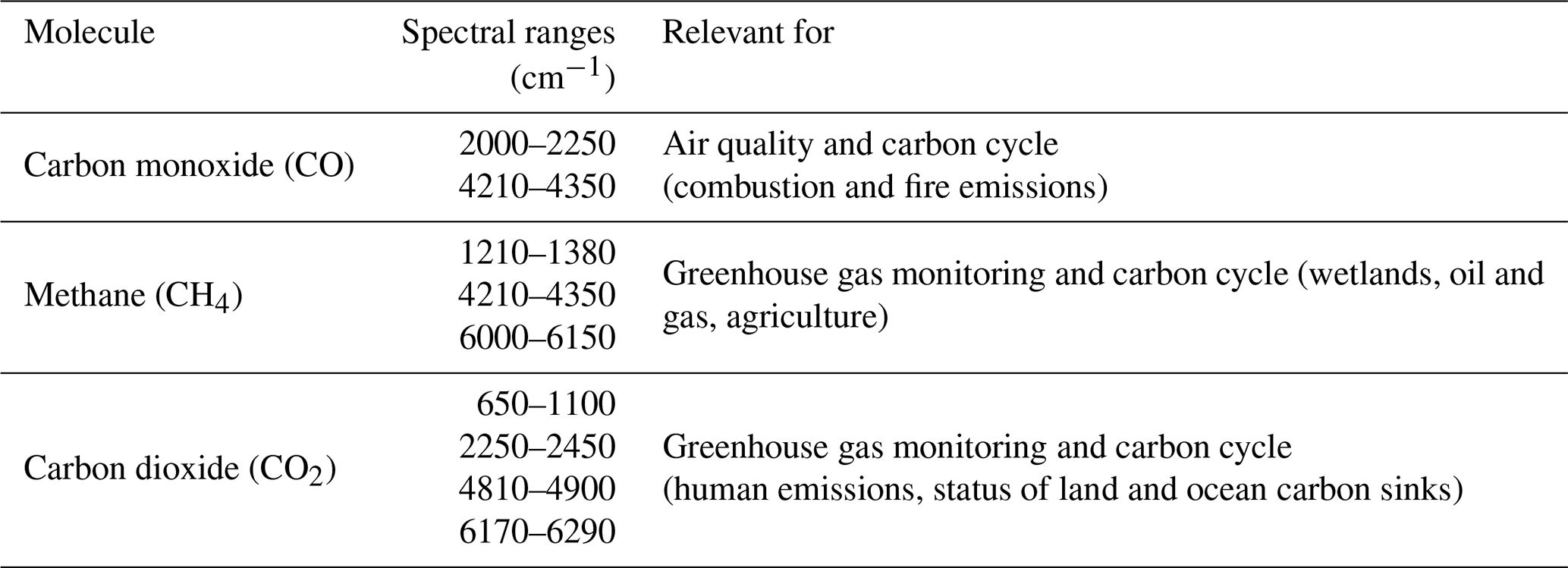
The Program of Record (PoR) of current and planned satellite observations, as described in the 2017 US Earth Science Decadal Survey (National Academies of Sciences, Engineering, and Medicine, 2018), includes a range of spectrally resolved radiance measurements in the thermal and shortwave infrared (TIR and SWIR) wavelength regions that provide key information on atmospheric temperature (TATM), water vapor (H₂O), and a range of trace gases (see Table 1 for a definition of spectral range designations). The TIR region can be further subdivided into mid-wave, longwave, and very longwave infrared (MIR, LWIR, and VLWIR) regions. Profiling of key gases including CO, CH₄, and CO₂ with sensitivity to planetary boundary layer (PBL) abundances was identified as a gap in current capability in the 2017 Decadal Survey, as was the promise of multispectral approaches for addressing this gap. In fact, combining radiances from the (thermal-emission-dominated) TIR and (solar-reflection-dominated) SWIR spectral regions has been shown to increase the vertical information content for these gases, providing improved information on near-surface variations relative to retrievals from the thermal alone (e.g., Christi and Stephens, 2004; Worden et al., 2010, 2015; Kuai et al., 2013; Fu et al., 2016; Zhang et al., 2018; Schneider et al., 2021). Such retrievals have the potential to extend the utility of satellite products for air quality forecasting, greenhouse gas monitoring, and carbon cycle research. In addition, combining TIR and SWIR infrared radiances also offers opportunities for increasing the vertical information of H₂O retrievals in the PBL, another topic highlighted by the Decadal Survey and by the NASA Decadal Survey PBL Incubation Study Team (Teixeira et al., 2021). Under clear-sky conditions, the SWIR provides sensitivity to H₂O (e.g., Noël et al., 2005; Trent et al., 2018; Nelson et al., 2016), CO (e.g., Buchwitz et al., 2004; Deeter et al., 2009; Landgraf et al., 2016; Borsdorff et al., 2017, 2018), CH₄ (e.g., Buchwitz et al., 2005; Frankenberg et al., 2006; Yokota et al., 2009; Hu et al., 2018; Parker et al., 2020) and CO₂ (e.g., Buchwitz et al., 2005; Yokota et al., 2009; O'Dell et al., 2018) throughout the full atmospheric column, providing complementary information to the TIR radiances that are strongly sensitive to the details of the profile of TATM, H₂O, and trace gases but have variable sensitivity to the PBL, depending on surface and atmospheric conditions.

Table 1 Spectral ranges and their designations used in this study.

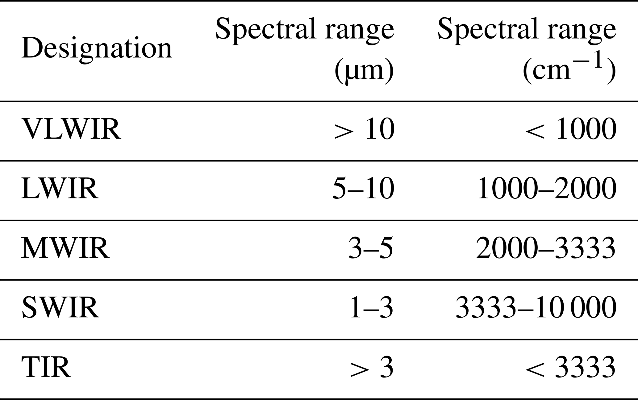
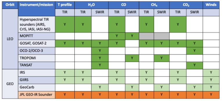
Table 2 shows a list of current and planned missions making spectrally resolved, spaceborne TIR and SWIR measurements. In low Earth orbit (LEO), the MOPITT instrument on the Terra platform has been providing a record of TIR + SWIR CO for over 2 decades (Buchholz et al., 2021). GOSAT provides spectrally resolved TIR and SWIR radiances on the same platform, with coverage of SWIR CO₂ and CH₄ bands, as well as H₂O absorption (Trent et al., 2018), but not SWIR CO. The TROPOMI instrument on the Sentinel-5P satellite flies in formation with the CrIS instrument on the Suomi-NPP satellite, providing nearly coincident observations of TIR and SWIR as well as presenting opportunities for multispectral retrievals of CO and CH₄. Measurements from geostationary (GEO) orbit can provide contiguous horizontal (∼4 km) and temporal (full sounding disk coverage in 1–2 h) resolution not possible from LEO (e.g., Schmit et al., 2009). The IRS instrument onboard the Meteosat Third Generation Sounder platform will track the four-dimensional structure of TATM and H₂O (Holmlund et al., 2021). The GIIRS instrument on the Fengyun-4 meteorological satellite has similar capabilities (Yang et al., 2017). Adkins et al. (2021) describe in comprehensive detail the value of a hyperspectral IR sounder in GEO orbit. Based on this report, an advanced high-resolution IR sounder has been recommended for the Geostationary Extended Observations (GeoXO) mission (https://www.nesdis.noaa.gov/next-generation-satellites/geostationary-extended-observations-geoxo, last access: 25 February 2022). However, none of the current or planned instruments and missions listed in Table 2 provide TIR + SWIR measurements from GEO on the same platform.

Table 2 Current and planned missions making spaceborne, spectrally resolved measurements of TIR and SWIR radiances. Note that MOPITT was designed to also offer measurements of CH₄, although that did not materialize (hence the gray shading).

Here, we describe an instrument concept, called the JPL GEO-IR Sounder, that would provide profiling of TATM, H₂O, CO, CH₄, and CO₂, as well as numerous other species important for air quality and the hydrological cycle, from a geostationary platform. The JPL GEO-IR Sounder is an imaging Fourier transform spectrometer that utilizes high-speed digital focal plane arrays to record simultaneous TIR and SWIR spectra from each pixel of the array (640×480 or 1024×1024 format). The primary advantages of this sounder include the following:

• coincident spatial and temporal retrievals of trace gases and TATM using both SWIR and TIR bands multiple times per day;

• combined TIR and SWIR retrievals provide for enhanced vertical resolution with PBL visibility for TATM, humidity, and multiple trace gases;

• capability for retrievals of 4D winds from combinations of TATM and H₂O temporal imagery as recently described using GIIRS data (Ma et al., 2021; Yin et al., 2021); and

• provision of data products that are not readily obtained by combining retrievals from PoR LEO and GEO sounders.

This paper is organized as follows: in Sect. 2, we describe the scenarios used in the simulations. Section 3 provides brief descriptions of the radiative transfer (RT), instrument, and inverse models. We discuss the considerations imposed on simulated JPL GEO-IR Sounder retrievals in Sect. 4. In Sect. 5, we present results for TATM, H₂O, and trace gas retrievals from simulated GEO-IR Sounder measurements for both individual spectral regions and combinations. The relevance of these simulated retrievals for observing system simulation experiments is discussed in Sect. 6. We arrive at some preliminary conclusions in Sect. 7. In particular, we show that the JPL GEO-IR Sounder would, for the first time, enable high-spatial- and temporal-resolution simultaneous retrievals in the TIR and SWIR, which together provide more vertical profile information and improved sensitivity to the PBL than either spectral region alone.

2 Scenarios

Representative atmospheric conditions, including TATM, H₂O and pollutant distributions, surface temperature, and other interferents, are needed to understand satellite instrument performance. Using the Weather Research and Forecasting model coupled to Chemistry (WRF-Chem) simulations at 4 km spatial resolution over the continental United States (Mary Barth, personal communication, 2012), we examined about 200 atmospheric profiles at six local times for 2 d in July 2006 over 17 locations that represent a range of diurnal meteorological conditions and a variety of air quality scenarios. For the purposes of these simulations, we assume clear-sky conditions. Simulation of conditions with significant aerosol loading and cloud interference adds significant complexity and is beyond the scope of this study. We calculate molecular absorption coefficients using the Line-By-Line Radiative Transfer Model (LBLRTM; Clough et al., 2005).

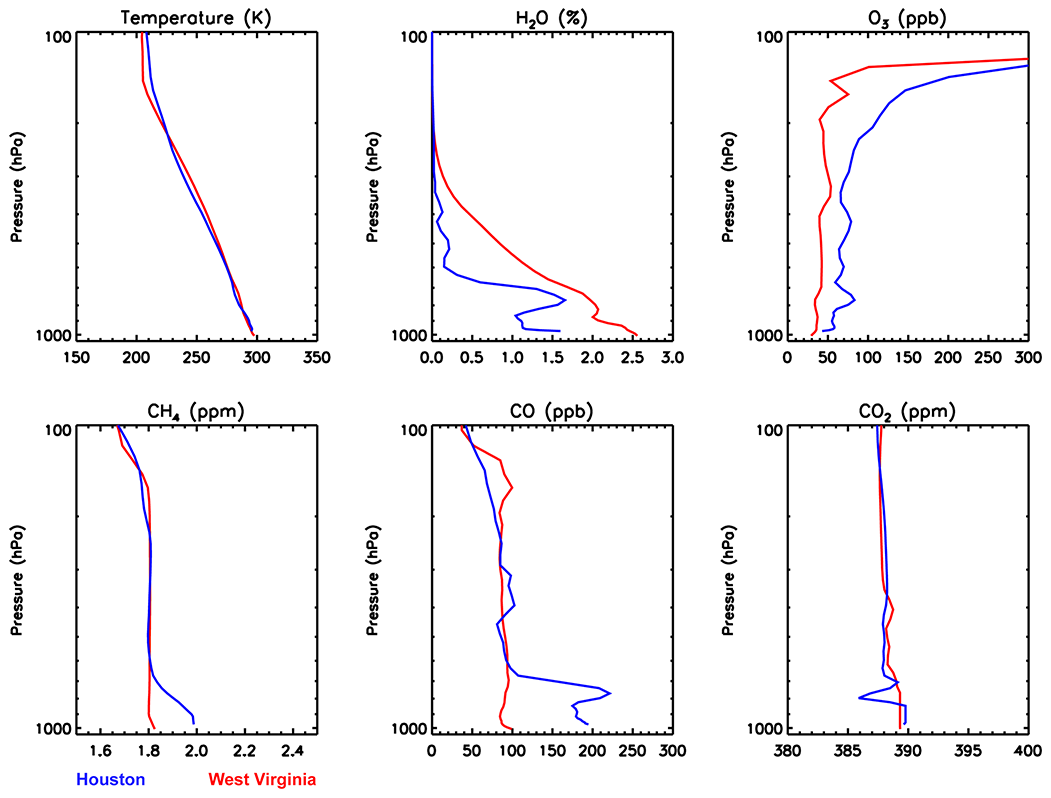
The main goal of these simulations is to evaluate the retrieval characteristics of TATM, H₂O, and trace gases for different instrument configurations. From our database of over 200 summertime atmospheric profiles over the continental US, we selected two representative daytime atmospheres: one near Houston to support the weather-focused observing system simulation experiment (OSSE) analyses and the background trace gas case and another in West Virginia that has more enhanced trace gas pollutants near the surface. Note that we kept the solar and viewing geometry as well as the surface albedo constant in order to isolate the effects of different boundary layer trace gas concentrations. Figure 1 shows the profile plots for TATM, H₂O, and trace gases that we examine in this paper (O₃, CO, CH₄, and CO₂) at the two locations.

Figure 1 Scenarios considered in the simulations.

The emissivity is obtained from a database structured by month and latitude–longitude coordinates. To populate the database, we used a global land use and land cover classification system developed by the US Geological Survey (Anderson et al., 1976) and mapped them into spectra from the ECOSTRESS spectral library (Baldridge et al., 2009; Meerdink et al., 2019; http://speclib.jpl.nasa.gov/, last access: 25 February 2022), as described in the TES Algorithm Theoretical Basis Document (Beer et al., 2002). The albedo is calculated from the emissivity using Kirchoff's law.

The location and times of the WRF-Chem profiles were used to calculate the solar viewing geometry, assuming a geostationary satellite at 95 W. The NOAA solar position calculator was used to verify the solar zenith and solar azimuth calculations (http://www.srrb.noaa.gov/highlights/sunrise/azel.html, last access: 25 February 2022).

3 Models

3.1 Radiative transfer model

We use the accurate and numerically efficient two-stream-exact-single-scattering (2S-ESS) RT model (Spurr and Natraj, 2011; Xi et al., 2015). This forward model is different from a typical two-stream model in that the two-stream approximation is used only to calculate the contribution of multiple scattering to the radiation field. Single scattering is treated in a numerically exact manner using all moments of the scattering phase function. High computational efficiency is achieved by employing the two-stream approximation for multiple-scattering calculations. The exact single-scattering calculation largely eliminates biases due to the severe truncation of the phase function inherent in a traditional two-stream approximation. Therefore, the 2S-ESS model is much more accurate than a typical two-stream model and produces radiances and Jacobians that are typically within a few percent of numerically exact calculations and in most cases with biases much less than a percent. This model has been widely used for the remote sensing of greenhouse gases and aerosols (Xi et al., 2015; Zhang et al., 2015, 2016; Zeng et al., 2017, 2018). Aerosols are not included in the analysis since the main objective was to investigate the impact of combining multiple spectral bands and of varying instrument parameters. However, the RT model has the capability of handling generic aerosol types.

The 2S-ESS RT model is used to generate monochromatic radiances at the top of the atmosphere for the atmospheric profiles and surface conditions near Houston over the entire spectral range considered for the JPL GEO-IR Sounder. Figure 2 shows the spectral radiance computed on a 0.002 cm⁻¹ wavelength grid. We also calculate the individual contributions of each absorbing gas to the radiance. The gaseous absorption features have different spectral distributions and line strengths, which can be used to identify spectral windows for profile retrievals and recognize interfering gases that also absorb strongly in the same channels.

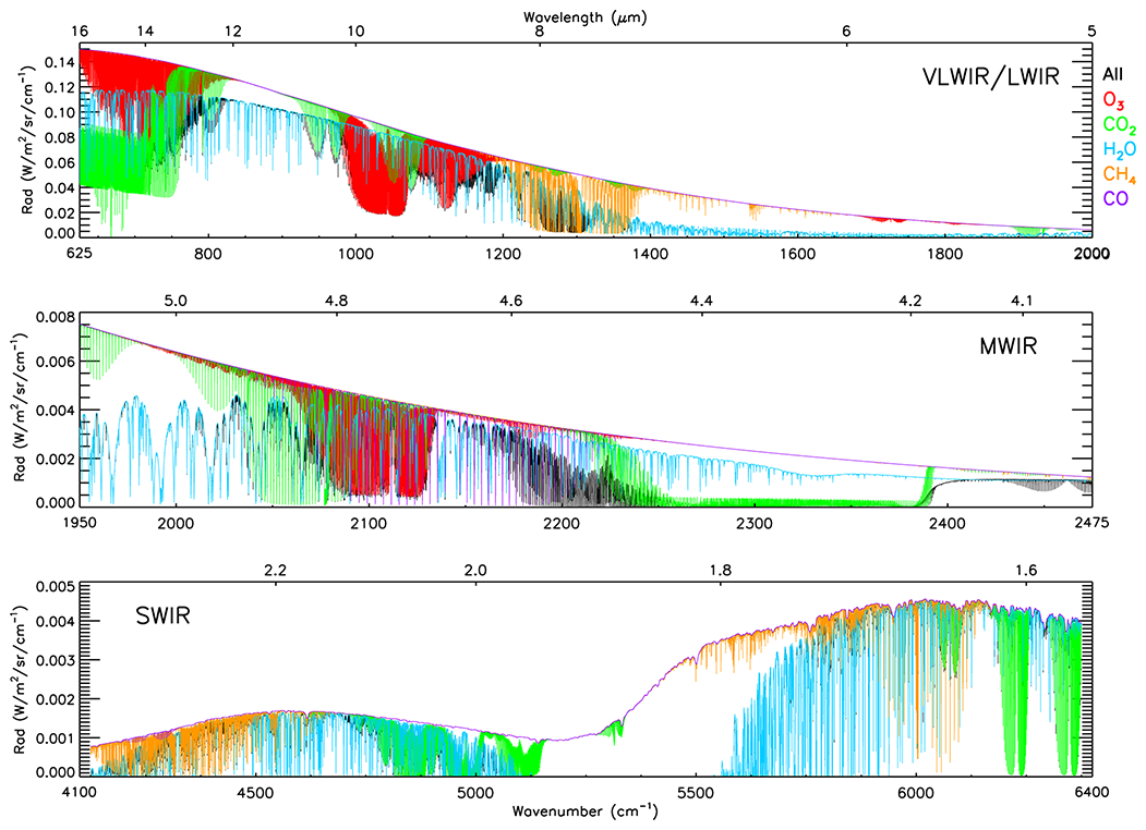
Figure 2 Simulated top-of-the-atmosphere monochromatic radiances (black) in the 650–7000 cm⁻¹ wavelength range for an atmospheric profile near Houston. Also shown are radiances corresponding to (red) O₃, (green) CO₂, (blue) H₂O, (orange) CH₄, and (purple) CO absorption.

3.2 Instrument model

This section starts with a brief description of the spectrometer, primarily to define the terms used in the instrument model. We then detail the focal plane arrays and the optical filter that determine the bandpasses of the instrument. The processing steps of the instrument model are then explained. Finally, we show some of the resulting spectra produced by the model.

3.2.1 Optics overview

The JPL GEO IR Sounder uses a Michelson interferometer, which modulates the light that passes through it. The interferometer is characterized by two main parameters: the spectral resolution, which is directly proportional to the maximum optical path difference (MOPD) between the two arms of the interferometer, and the optical throughput or étendue, which is given by the product of the area of the aperture stop and the angular field of view (AΩ). From geostationary orbit, a ground pixel of 2.1 km subtends an angle of 58.7 µrad, and for a focal plane array (FPA) of 1024×1024 pixels, the overall FOV is 60 mrad; this fits well within the Fourier transform spectrometer (FTS) design parameters. In parallel with the light from the target scene, a beam from an internal metrology laser travels through the interferometer. This laser is used to precisely measure the optical path difference to within a small fraction of the laser wavelength. An imaging FTS (IFTS) shares many of the principles of the traditional FTS; the main difference is that the detector is replaced with an FPA. The main challenge in the IFTS design is in the FPA, which must operate at a high frame rate (0.5–1 kHz) and high dynamic range (14–16 bits) to properly digitize the interferograms.

3.2.2 Focal plane arrays

The JPL GEO-IR Sounder FPA optics use a dichroic to split the interferometer output along the wavelength dimension: radiation from 1 to 5.3 µm is sent towards FPA 1, and radiation from 5.3 to 15.4 µm is directed to FPA 2. Whereas FPA 2 is a single-color detector handling its full domain at all times, FPA 1 is a dual-color detector. The two colors of FPA 1 are operated sequentially, recording either the 1 to 3 µm domain (SWIR; FPA 1a) or the 3 to 5.3 µm domain (MWIR; FPA 1b). This dual-color operation is implemented inside the FPA by having two distinct detectors in an optical “sandwich”. It is designed to minimize the effect of photon noise in the low-light MWIR and SWIR domains. Furthermore, the SWIR FPA 1a bandpass is narrowed by a triple-band optical filter tailored to the regions that contain absorption bands of interest (Fig. 3). As listed in Table 3, the SWIR domains of interest are (1) 4210–4350 cm⁻¹, (2) 4810–4900 cm⁻¹, (3) 6000–6150 cm⁻¹, and (4) 6170–6290 cm⁻¹. Based on previous optical filter studies, we allow 200 cm⁻¹ for the filter slope on either side. Since the gap between the first two domains would therefore be small and the signal there is low, these have been merged (4210–4900 cm⁻¹). Domains (3) and (4) have also been combined (6000–6290 cm⁻¹). In addition, the 1.27 µm oxygen band (7780–8010 cm⁻¹) will be used to measure the light path. We believe that it is best to specify the 50 % transmission points for the filter bands, as that is where the slope is maximum and hence most easily verified. With a 200 cm⁻¹ transition region, the 50 % point will be 100 cm⁻¹ outside the bandpasses. Hence, the final triple-band filter configuration is 4110–5000 cm⁻¹ (2.000–2.433 µm), 5900–6390 cm⁻¹ (1.565–1.695 µm), and 7680–8110 cm⁻¹ (1.233–1.302 µm). The triple-band filter physically covers the two-color FPA 1. It is intended to limit the photon flux only in the SWIR mode of operation, with the detector that is sensitive over the 1–3 µm domain (FPA 1a). The filter must also be transparent over the 3–5.3 µm domain of the other shared detector (FPA 1b). It may be possible to combine the first band of the triple-band filter (2–2.433 µm) with this MWIR transparency need (3–5.3 µm), but this has not been simulated in this study.

Table 3 Spectral ranges used in this study for simulated retrievals of CO, CH₄, and CO₂.

3.2.3 Instrument model description

The instrument model for the JPL GEO IR Sounder allows us to explore the instrument trade space and its effect on retrieved atmospheric composition. It includes the ability to convolve synthetic spectra and Jacobians with the instrument line shape (ILS). The model performs the following steps.

1. It reads synthetic data from the radiative transfer model. The radiance spectrum is extended using blackbody curves simulating the Earth and the Sun, and it is converted to a photon flux spectrum. After this step, the spectrum is in units of photons m⁻² sr⁻¹(cm⁻¹)⁻¹ s⁻¹.

2. It convolves the spectrum with the theoretical FTS ILS, given as 2Lsinc(2σL), where L is the MOPD and sinc$\left(x\right)=\sin \left(\mathit{\pi }x\right)/\mathit{\pi }x$. This expression of the ILS has unit area, and hence the convolution does not change the overall magnitude or the units of the spectrum. It does, however, reduce the spectral resolution, broadening all sharp features. In the same step, we resample the spectrum on a coarser grid; i.e., we “decimate” the spectrum. For example, in the current simulations, we reduce the wavenumber interval by a factor of 50 from 0.002 to 0.1 cm⁻¹.

3. It scales the spectrum by the étendue of the instrument. After this step, the units of the spectrum are photons (cm⁻¹)⁻¹ s⁻¹.

4. It applies further scaling to account for the single output design (whereby half the light is sent through the instrument and the other half sent back to the source), losses in the metallic coatings and at the uncoated optical interfaces (i.e., compensator and back side of beamsplitter), the efficiency of the beamsplitter coating, the quantum efficiency of the detector, and the integration time of the analog-to-digital converter. After this step, the units of the spectrum are photoelectrons per wavenumber.

5. It applies bandpass limits caused either by an optical filter or the working domain of the detector.

6. It applies the Fourier transform to convert the spectrum into an interferogram.

7. It computes the number of photoelectrons counted in each interferogram data sample. From this, we can compute the photon noise. Subsequently, white noise is added to the interferogram with a root mean square amplitude matching the computed photon noise.

8. It simulates the interferogram digitization, which is performed for each pixel within the read-out integrated circuit of the two FPAs.

9. It produces the final spectrum by Fourier transform. The signal-to-noise ratio (SNR) is then evaluated by computing the noise level in blacked-out regions on either side of the instrument bandpass and by locating the maximum signal within the bandpass.

3.2.4 Spectral results

Figure 3 shows a JPL GEO-IR Sounder model spectrum for FPA 1a, covering the SWIR domain. Figure 4 shows a similar spectrum for the VLWIR, LWIR, and MWIR FPA bands: FPA 2 covers the VLWIR and LWIR domains, and FPA 1b covers the MWIR domain. The spectral ranges include the range utilized by existing TIR sounders (AIRS, CrIS, IASI) and selected bands in the SWIR. In particular, the FPA 2 spectral range contains critical information for radiance assimilation by weather forecasting algorithms (see, e.g., Eresmaa et al., 2017). The spectral resolution (MOPD) of the JPL GEO-IR Sounder is configurable. For these simulations, we choose to look at three possible MOPD options: a CrIS-like spectral resolution (0.8 cm MOPD, 0.625 cm⁻¹ resolution, described as nominal spectral resolution or NSR in Table 4), an intermediate option (2 cm MOPD, 0.25 cm⁻¹ resolution), and a high-spectral-resolution option (5 cm MOPD, 0.1 cm⁻¹ resolution, described as full spectral resolution or FSR in Table 4). In order to make an “apples to apples” comparison, we consider the same integration time (1 ms per interferogram point) for these three options. The integration time is driven by the high-spectral-resolution option. The native and binned (footprint-averaged) ground sampling distance (GSD) is also indicated in Table 4.

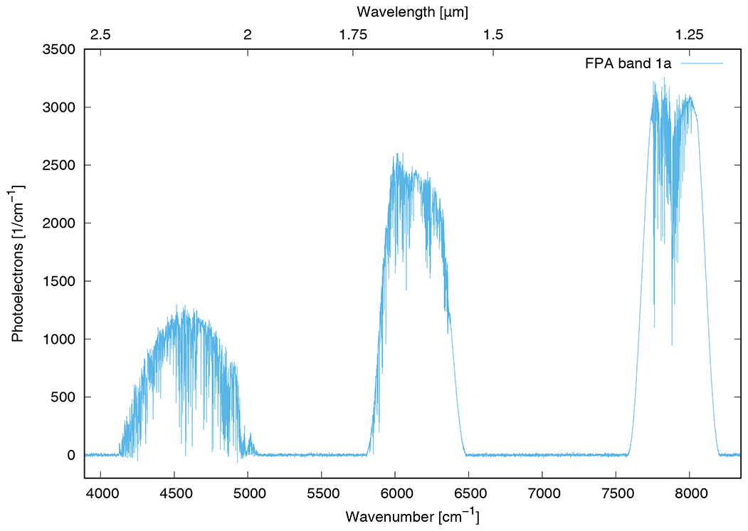
Figure 3 Simulated JPL GEO-IR Sounder spectrum in the SWIR domain. The SWIR domain is subdivided into discrete bands using a triple-band interference filter to maximize the SNR in spectral regions of interest (CO₂, CH₄, CO, H₂O, and O₂).

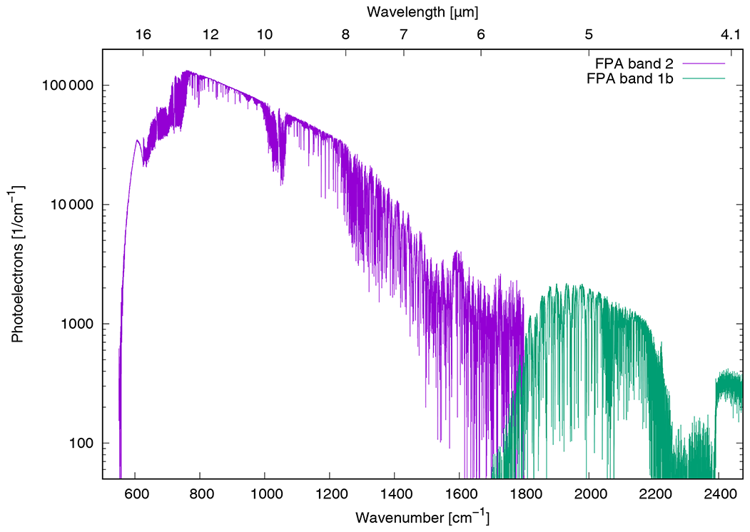
Figure 4 Simulated JPL GEO-IR Sounder spectrum in the VLWIR, LWIR, and MWIR domains. Note the logarithmic scale.

Table 4 Comparison of the JPL GEO-IR Sounder with other state-of-the-art instruments.

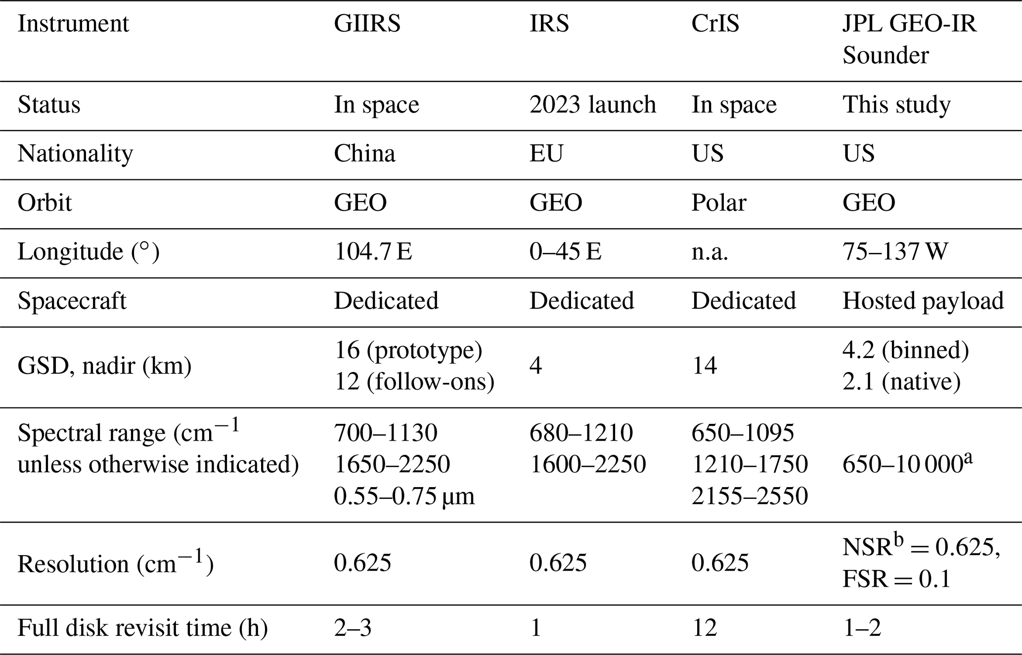
^a FTS instrument capability. ^b NSR: nominal spectral resolution. FSR: full spectral resolution. FSR mode decreases retrieval biases caused by interfering absorbers.

3.3 Inverse model

We use an optimal estimation approach (Rodgers, 2000) and perform linear retrievals from simulated radiances described in the previous section. The spectral differences of the modeled and satellite-measured radiances and the differences of the species profile and the a priori profile are mathematically minimized: weighted by the measurement error and the a priori constraint. The species profile can then be optimally derived.

The a priori constraint vectors for TATM and H₂O are obtained from forecast fields from the NASA Global Modeling and Assimilation Office, supplied for use within the TES retrieval algorithm (Bowman et al., 2006). A priori constraint matrices are constructed using the method described in Kulawik et al. (2006) from an altitude-dependent combination of zeroth-, first-, and second-order derivatives of the profiles. For TATM and H₂O, the square roots of the diagonals of the respective constraint matrices are on the order of 1.8–2.2 K and 15 %–18 %, respectively. A priori vectors for O₃, CO, and CH₄ are taken from calculations using the Model for OZone And Related chemical Tracers (MOZART3) (Brasseur et al., 1998; Park et al., 2004) that were performed for the purpose of construction of trace gas climatologies for the Aura mission. For O₃, the square root of the diagonal of the constraint matrix is on the order of 25 % in the troposphere, 40 % in the stratosphere, and 15 % above. For CO, this is set to 30 % over the entire atmosphere, while for CH₄, the values range from 2 %–10 %. The constraint matrices for CO are the same as those used by the MOPITT algorithm (Deeter et al., 2010). For CO₂, the a priori vector and constraint used are described in Kulawik et al. (2010). The square root of the diagonal of the constraint matrix ranges from 1.2 %–2 %. We note that these profile constraints were developed for TIR instruments and therefore may not capture strong near-surface variability. There could be scope for increasing the near-surface information content via development of updated constraints, although that work is outside the scope of this study.

The end-to-end retrieval analysis provides averaging kernels, which describe the sensitivity of the retrieved atmospheric state to the true state; degrees of freedom for signal (DOFS), which denote the pieces of vertical information contained in the retrieved profile; and retrieval errors. These metrics are used for evaluating the retrieval results for a variety of spectral bands as well as spectral and spatial resolutions.

4 Considerations for simulated retrievals

For the retrieval simulations described here, we consider a somewhat idealized scenario. Simulations have been performed for clear-sky, no-aerosol conditions. In retrievals from actual measured radiances, even for a clear-sky, non-scattering atmosphere, there is always some forward model error due to, e.g., uncertainties in spectroscopy, interfering species, and the treatment of the surface. With real data, these kinds of uncertainties can lead to significant systematic errors in the retrievals, particularly for well-mixed greenhouse gases such as CH₄ and CO₂. For the simulations presented here, we have considered only the error term associated with measurement noise.

The measurement noise associated with the simulated radiance is obtained using the instrument model described in Sect. 3.2. The JPL GEO-IR Sounder concept is configurable in terms of spectral range and spectral resolution, with a native spatial resolution that corresponds to a 2.1 km footprint on the ground. Different configurations of the instrument concept will affect the number of photons available in each channel and therefore impact the SNR. For a given integration time, lower spectral resolution leads to correspondingly higher SNR. The SNR of the observed radiance spectra can be increased by increasing the integration time. For geostationary observations, this leads to a trade-off between measurement noise and temporal resolution. An increase in the throughput (étendue) leads to lower noise (Schwantes et al., 2002).

In retrievals from real data, higher spectral resolution can offer advantages in terms of ability to distinguish between the target molecule and interfering spectral signatures from other molecules with features in the spectral range of interest, despite the increase in measurement noise. In the results presented in this study, that advantage in reduction of systematic error is not accounted for. The SNR can also be increased by aggregating spatially. For example, aggregating four 2.1 km footprints would increase the SNR by a factor of 2. Depending on the application of the measurements, there may be some advantage to trading spatial resolution for a gain in SNR.

5 Results

5.1 TATM and H₂O retrievals

High spectral resolution is necessary to provide the vertically resolved TATM and H₂O information critical for numerical weather prediction and for many other applications including local extreme weather conditions and global climate change. Current satellite-based TATM and H₂O retrievals mainly utilize TIR spectral measurements. Here we also examine information gained from adding SWIR measurements. Tables 5 and 6 list the possible choices of frequency range for TATM and H₂O retrievals. Some of these spectral ranges are used in current operational missions, while some are candidates for future missions. We compare results for three values of spectral resolution and for two values of spatial resolution.

Table 5 DOFS for TATM retrievals for three spectral (MOPD) and two spatial (GSD) resolution scenarios. The values shown here are for the Houston profile.

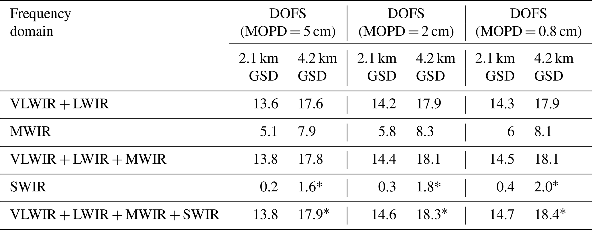
^* Instrument noise is reduced by a factor of 5 through footprint averaging for the SWIR only, providing an effective GSD of 21 km.

Table 6 Same as Table 5 but for H₂O.

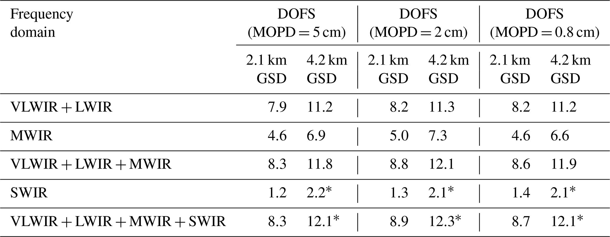
^* Instrument noise is reduced by a factor of 5 through footprint averaging for the SWIR only, providing an effective GSD of 21 km.

Examining the above DOFS tables, we see competing effects of spectral resolution (MOPD) and measurement noise. As described in Sect. 3.2, the measurement noise (noise-equivalent spectral radiance, NESR) is estimated for a fixed integration time for both the 2.1 and 4.2 km ground sampling distance (GSD) configurations. The NESR for the MOPD =0.8 cm instrument is therefore smaller than that for the MOPD =2 or 5 cm instruments. Typically, however, the higher-spectral-resolution instruments provide larger DOFS than the NSR instrument. For H₂O retrievals, the optimal DOFS are provided by the intermediate-resolution instrument.

The differences in DOFS for the two GSD values are obvious. This shows the trade-off between spatial resolution and retrieval vertical resolution as well as precision (not listed). Both GSDs provide high-precision, high-vertical-resolution TATM and H₂O retrievals. We estimate the tropospheric vertical resolution for TATM to be 1.5–2 km with <0.5 K precision and for H₂O to be 1–2 km with ∼5 % precision. In comparison, representative tropospheric values for AIRS are 1 km for TATM and 2 km for H₂O (Irion et al., 2018).

The selection of spectral regions also affects the TATM and H₂O products. For example, using the VLWIR + LWIR + MWIR domain provides much more sensitivity compared to using MWIR alone. Figure 5 shows averaging kernel plots for TATM and H₂O for the 4.2 km GSD option for four spectral band combinations: VLWIR + LWIR, MWIR, SWIR, and VLWIR + LWIR + MWIR + SWIR. The characteristics of the TIR TATM and H₂O retrievals are very similar to those obtained by currently operating instruments. We note that the sensitivity of SWIR retrievals is mostly near the surface. Further, the measurement noise in the SWIR was reduced by a factor of 5 in these figures by averaging 25 pixels, thereby reducing the effective GSD to 21 km. Note that this is worse than the 15 km AIRS/CrIS native resolution but better than the 45 km that the TATM and H₂O products are typically reported on. Further, while 5×5 pixels may be required for trace gas retrievals in the SWIR (see Sect. 5.2), which is therefore a little worse than AIRS/CrIS, we measure TIR and SWIR at the same time, eliminating bias from observing with separate instruments.

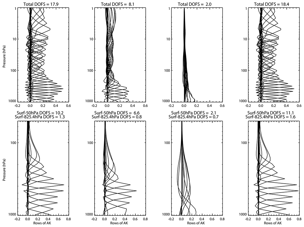
Figure 5 Plots of averaging kernel rows for (top) TATM and (bottom) H₂O. The spectral ranges are (from left to right) VLWIR + LWIR, MWIR, SWIR, and VLWIR + LWIR + MWIR + SWIR. These results are for the Houston case.

5.2 Trace gas retrievals

Among many possible detectable trace gases from the extended spectral radiance measurements, we selected to examine profile retrieval characteristics for O₃, CO, CH₄, and CO₂ for the given instrument configurations (see Table 3 for retrieval spectral ranges). Table 7 lists DOFS for the chosen trace gases for the West Virginia scenario. Results for the FSR option are largely similar to those for the intermediate-spectral-resolution instrument and are hence not shown. The DOFS in Table 7 are broadly consistent with previously published work on species profile retrievals from satellite observations (Beer, 2006; Connor et al., 2008; Deeter et al., 2009, 2015; George et al., 2009; Kulawik et al., 2010; Worden et al., 2010, 2013; Clerbaux et al., 2015; Fu et al., 2016; Smith and Barnet, 2020). For a given spectral resolution instrument, the higher DOFS in retrievals for the larger GSD case for all species are due to the reduced measurement noise. For a given GSD, the DOFS are slightly higher for the NSR case compared to the MOPD =2 cm case, but the differences are small. It is worth reiterating that these simulated retrievals represent an idealized scenario in which we assume perfect knowledge of interfering species in the spectral range for any given target species. In this scenario, with a constant integration time, the NSR option provides results similar to the MOPD =2 cm option due to the trade-off between spectral resolution and instrument noise.

Table 7 Trace gas retrieval configurations and DOFS for the West Virginia profile. TATM and H₂O are simultaneously retrieved when listed.

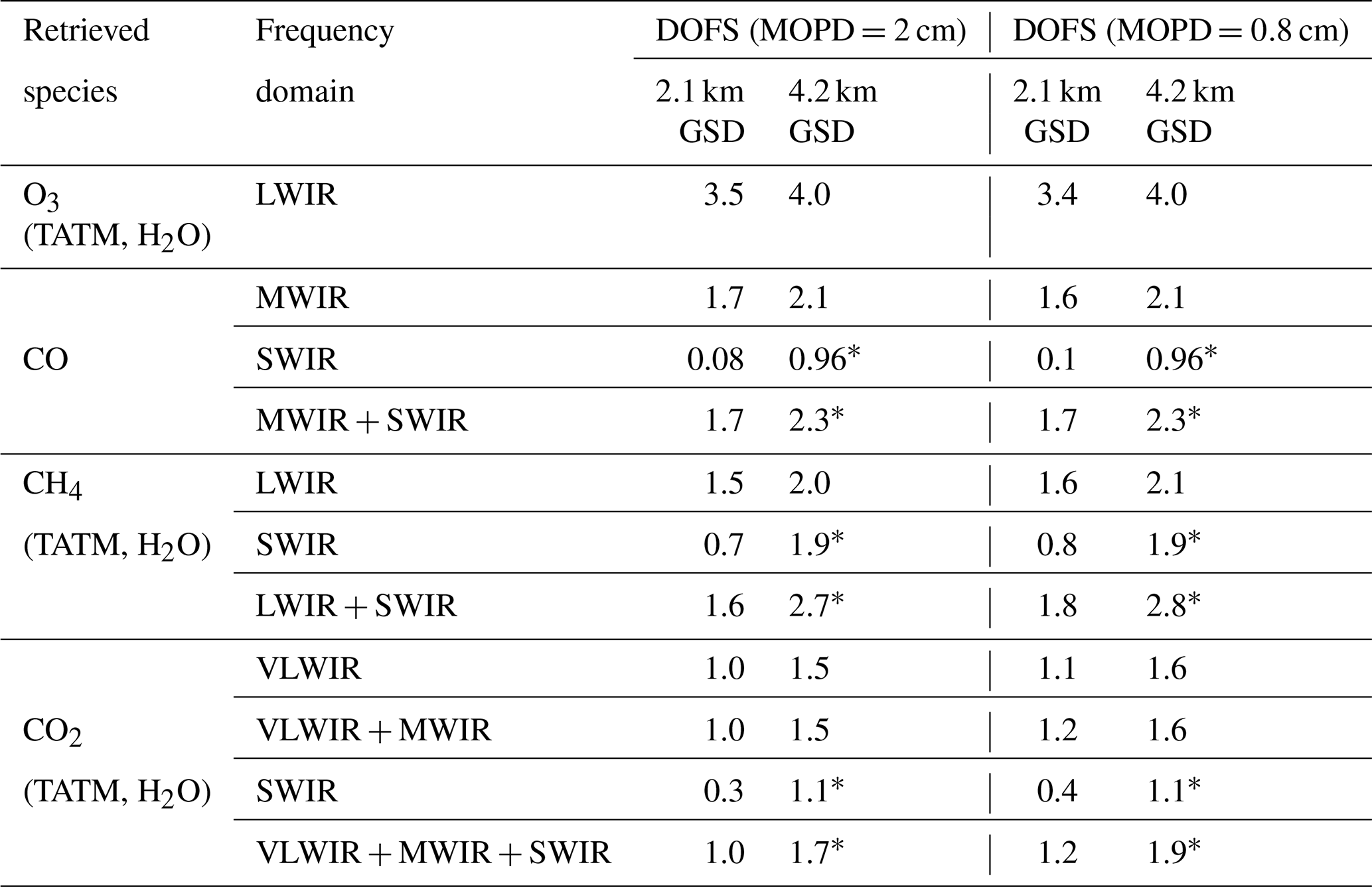
^* Instrument noise is reduced by a factor of 5 through footprint averaging for the SWIR only, providing an effective GSD of 21 km.

Figure 6 shows averaging kernel plots for CO for MWIR- and SWIR-only scenarios and for combined MWIR + SWIR retrievals. The combination of wavelength regions provides improved sensitivity to the lower troposphere compared to either spectral region alone. CO₂ retrievals (Fig. 7) benefit the most from the combination of VLWIR + MWIR + SWIR retrievals. The SWIR domain adds sensitivity in the lower troposphere and near the surface. The characteristics of the CO₂ retrievals are in good agreement with OCO-$\mathrm{2}/\mathrm{3}$ observations. For CH₄ (Fig. 8), the addition of SWIR bands also provides noticeable enhancement in lower tropospheric and near-surface sensitivity. For CO retrievals, the contribution of the SWIR to the near-surface sensitivity is less pronounced. The stronger contribution of SWIR measurements to the total DOFS for CH₄ and CO₂ compared to CO is a result of three factors: (1) lower top-of-the-atmosphere solar irradiance in the CO spectral region relative to the CH₄ and CO₂ regions, (2) lower surface albedo, and (3) larger absorption, primarily by H₂O and CH₄. Our results for O₃ are broadly consistent with published results for LWIR satellite observations (e.g., Nassar et al., 2008; Smith and Barnet, 2020). Figures 6–8 use the same effective GSD of 21 km in the SWIR as described in Sect. 5.1.

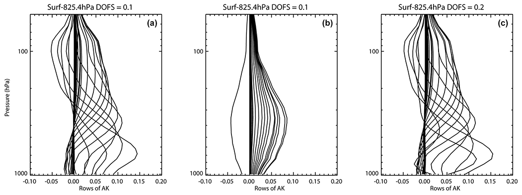
Figure 6 Plots of averaging kernel rows for CO retrievals. The spectral ranges are (from a to c) MWIR, SWIR, and MWIR + SWIR. These results are for the West Virginia case.

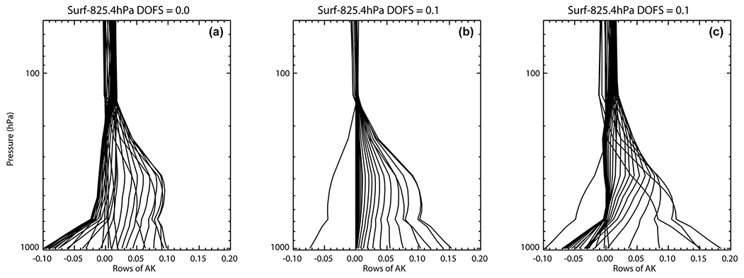
Figure 7 Plots of averaging kernel rows for CO₂ retrievals. The spectral ranges are (from a to c) VLWIR + MWIR, SWIR, and VLWIR + MWIR + SWIR. These results are for the West Virginia case.

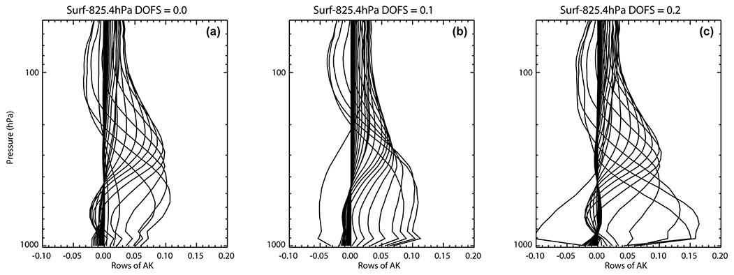
Figure 8 Plots of averaging kernel rows for CH₄ retrievals. The spectral ranges are (from a to c) LWIR, SWIR, and LWIR + SWIR. These results are for the West Virginia case.

6 Discussion: use of GEO-IR information in data assimilation and observing system simulation experiments

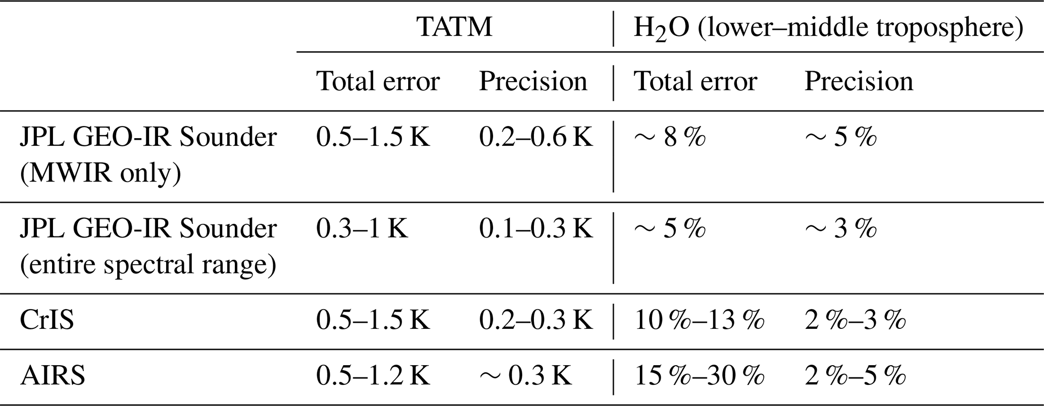
We have focused in this paper on the characteristics of the measurements and retrievals that we expect to obtain from the GEO-IR observing platform. While this paper does not deal directly with the use of this information in a data assimilation system, the results we have presented lay the necessary groundwork for future work in this area. In particular, the detailed characterization of uncertainties in the TATM and H₂O retrievals provided by this study can be directly incorporated into a set of weather forecast OSSEs. We have begun this research and will report on the results in a subsequent paper. Note that for a weather forecast OSSE to be credible, it is crucial to represent the synthetic measurements as accurately as possible. TATM and H₂O precision and total error are reported in Table 8; it can be seen that the errors for the MWIR-only configuration are on the order of the errors in CrIS and AIRS retrievals, while the full-spectrum JPL GEO-IR Sounder configuration yields total errors that are smaller than those from either CrIS or AIRS. As such, assimilation of information from JPL GEO-IR Sounder measurements is expected a priori to have as much or greater impact on weather forecasts compared with existing hyperspectral sounders. Note that the total error in the full-spectral-range TATM and H₂O retrievals is equivalent to, or less than, the uncertainty reported for radiosonde measurements of these quantities (Rienecker et al., 2008, Table 3.5.2).

Table 8 Estimates of total and precision errors for JPL GEO-IR Sounder, CrIS, and AIRS TATM and H₂O retrievals in the troposphere. Note that data used for CrIS and AIRS retrievals were obtained near Houston, Texas, in August 2020. Averaged retrieved cloud optical depths are limited to less than 0.1, consistent with mostly clear-sky conditions.

We also note that there will be particular advantages and challenges in assimilating the high-temporal-resolution data that will be available from the JPL GEO-IR Sounder. The clear advantage is the ability to observe rapidly evolving processes (e.g., the environment around thunderstorms and hurricanes; see, e.g., Li et al., 2018). This information is not available from the current LEO constellation. However, many modern data assimilation systems are configured for assimilation of intermittent data (at best hourly in operational data assimilation systems). While four-dimensional variational data assimilation (4D-Var) is capable of ingesting data at non-synoptic times, assimilation of sub-hourly data remains challenging. It is likely that all but the most rapid-update data assimilation systems will require modification to make best use of the high-time-frequency geostationary soundings provided by the JPL GEO-IR Sounder.

7 Conclusions

In this paper, we present an end-to-end retrieval study for a proposed FTS instrument covering the entire infrared spectral range from 1–15 µm from a geostationary satellite orbit. An instrument model is used to derive realistic measurement radiance and noise for several diurnal observations over small ground footprints (e.g., 2.1 km). We perform TATM and trace gas profile retrievals for the JPL GEO-IR Sounder that covers the entire VLWIR, LWIR, MWIR, and SWIR spectral domains. Retrieval characteristics, such as DOFS and measurement error, are examined in order to evaluate the performance of several instrument configurations. These configurations include VLWIR-, LWIR-, MWIR-, and SWIR-only, their combinations, and different spectral and spatial resolutions for a realistic geostationary observing system making field-of-view observations at fixed time intervals. Two summertime atmospheres are used: a scenario near Houston as a clean-air case and one in West Virginia representing a polluted scenario. We analyze TATM, H₂O, O₃, CO, CH₄, and CO₂ profile retrievals.

High spectral resolution can provide improved ability to distinguish absorption lines of the target species from interferents. In the case of species (such as O₃) for which much of the total column lies in the stratosphere, higher spectral resolution also provides enhanced ability to separate the tropospheric signal from the stratospheric signal. When the total integration time is fixed, there is a trade-off between spectral resolution and noise. In the idealized retrievals presented here, we assume perfect knowledge of interfering species. In this case, three different MOPDs provide comparable results in terms of DOFS. However, in the real world, we would expect higher spectral resolution to offer advantages in terms of reduction in systematic errors.

Compared to single-spectral-region instruments, e.g., only LWIR or MWIR, combinations of VLWIR, LWIR, MWIR, and SWIR enhance the sensitivity of the retrievals to the lower troposphere. In our analyses, we find that the contributions from the SWIR in the combined measurements are noticeable for both trace gas and TATM retrievals, especially when the ground pixels are averaged to reduce measurement noise in the SWIR. In particular, the SWIR measurements add information in the lower troposphere and for near-surface species retrievals.

We limit the spatial resolution choices to GSD =2.1 and 4.2 km in our simulations. Especially for multi-band retrievals, the results are realistically adequate for many research applications for both ground sampling footprints. We compare performance metrics (e.g., NESR and SNR) for the proposed instrument with values for several current and past satellite instruments in multiple spectral bands. The performance of the JPL GEO-IR Sounder is similar to or better than currently operational instruments. At the same time, the JPL GEO-IR Sounder provides much higher spatial and temporal resolution as well as a wider range of trace gases than current instruments that combine TIR and SWIR. The derived retrieval characteristics (e.g., DOFS and retrieval errors) also compare favorably with currently available products.