Modelling the spectral shape of continuous-wave lidar measurements in a turbulent wind tunnel

This paper describes the development of a theoretical model for the turbulence spectrum measured by a short-range, continuous-wave lidar (light detection and ranging). The lidar performance was assessed by measurements conducted with two WindScanners in an open-jet wind tunnel equipped with an active grid, for a range of different turbulent wind conditions. A hot-wire anemometer is used as reference to assess the lidar's measured statistics, time series and spectra. In addition to evaluating the statistics, the correlation between the time series and the root-mean-square error (RMSE) on the wind speed, the turbulence spectrum measured by the lidar is compared with a modelled spectrum. The theoretical spectral model is applied in the frequency domain, using a Lorentzian filter in combination with Taylor's frozen turbulence hypothesis for the probe length averaging effect and an added white noise term, evaluated by qualitatively matching the lidar measurement spectrum. High goodness-of-fit coefficients and low RMSE values between the hot wire and WindScanner were observed for the measured time series. The correlation showed an inverse relationship with the prevalent turbulence intensity in the flow for cases with a comparable power spectrum shape. Larger flow structures can be captured more accurately by the lidar, whereas small-scale turbulent flow structures are partly filtered out as a result of the lidar's probe volume averaging effect. It is demonstrated that an accurate way to define the cut-off frequency at which the lidar's power spectrum starts to deviate from the hot-wire reference spectrum is the frequency at which the coherence drops below 0.5. This coherence-based cut-off frequency increases linearly with the mean wind speed and is generally an order of magnitude lower than the probe length equivalent cut-off frequency, estimated according to a simple model based on the full width at half maximum (FWHM) of the laser beam intensity along the line of sight and assuming Taylor's frozen turbulence hypothesis. A convincing match between the modelled and the measured WindScanner power spectrum was found for various different cases, which confirmed that the deviation of the lidar's measured power spectrum in the higher frequency range can be analytically explained and modelled as a combination of a Lorentzian-shaped intensity function and white noise in the lidar measurement. Although the models were developed on the basis of wind tunnel measurements, they should be applicable to atmospheric boundary layer field measurements as well.

1 Introduction

Wind tunnels are frequently used to reproduce wind conditions more realistically, for example, in order to perform meaningful model wind turbine tests (Campagnolo et al., 2016; Tian et al., 2018; Berger et al., 2021). Existing wind tunnels can simulate the neutrally stratified atmospheric boundary layer through passive flow manipulation by means of roughness elements and spires, one example being the facility at the Polytechnic University of Milan (Bottasso et al., 2014). Other wind tunnels, such as the wind tunnel of the University of Oldenburg, are equipped with an active grid which can generate user-defined wind conditions, for example, wind shear and turbulence (Kröger et al., 2018; Neuhaus et al., 2020, 2021).

These complex wind conditions require equally sophisticated ways of measuring the flow in the wind tunnel. Hot-wire anemometers (Bradshaw, 1971; Comte-Bellot, 1976) have a high temporal resolution and can measure one to three wind speed components at a single point in space. Particle image velocimetry (PIV) can be used to measure a highly resolved two-dimensional wind flow over a small area of interest (Adrian and Westerweel, 2011). Laser Doppler anemometers (LDAs) use the Doppler effect in order to remotely measure one, two or three wind speed components by focusing a monochromatic, coherent laser at a single point in space (Durst et al., 1976).

The continuous-wave (CW) lidar (Slinger and Harris, 2012; Pitter et al., 2013) is also a laser-based Doppler anemometer. These coherent-detection-based lidars measure the line-of-sight component of the wind speed and have a slightly lower temporal and spatial resolution than the two aforementioned sensors but are, on the other hand, a non-invasive and flexible scanning measurement technique. In contrast to the other aforementioned sensors, lidar technology was originally developed for real-scale studies. The execution of lidar measurements inside a wind tunnel (Pedersen et al., 2012; van Dooren et al., 2017; Sjöholm et al., 2017; Hulsman et al., 2020) is a relatively novel and challenging concept, which we believe to become a benchmark for the measurement of the flow through and at cross-sections inside a wind tunnel, either with or without model wind turbines interacting with the flow.

Previous research on the effect of the lidar's effective probe length averaging and range gating on the measurement spectrum focuses mainly on the spectral transfer function. Angelou et al. (2012) propose two different ways of modelling the spectral transfer function between lidar and sonic anemometer time series. Held and Mann (2018) investigate the effect of the line-of-sight velocity determination method on the shape of the spectral transfer function. Puccioni and Iungo (2021) propose a spectral correction for the range-gate averaging effect of pulsed lidars, based on a simple low-pass filter fitted to the lidar's frequency spectrum. In this paper we implement a similar approach for a CW lidar; however, we use an analytical approach to model the lidar's measured spectrum that includes a minimal amount of a priori information from the lidar measurement itself.

Consequently, the main objective of this paper is to address the performance and the limitations of using short-range lidar for turbulence measurements, by modelling, comparing and evaluating the measurement principle in the frequency domain. This is addressed by analysing the following three aspects:

1. the correlation between the lidar and hot-wire time series, quantified with the linear regression goodness-of-fit coefficient;

2. the mean average error and root-mean-square error on the mean wind speed, quantified with respect to the hot wire;

3. the comparison between the CW-lidar and hot-wire measurement in the frequency domain, quantified by two different definitions for the cut-off frequency of the turbulence spectrum.

Apart from these three quantitative properties, an analytic model is applied to qualitatively model the shape of the lidar's measured spectrum and its difference with respect to a reference, in this case the hot-wire measurement spectrum.

The structure of the paper is as follows: Sects. 2 and 3 are both part of the methodology, describing the measurement equipment and setup, and the physical models developed in this study, respectively. Section 4 presents and immediately discusses the results of the implementation of said physical models, and Sect. 5 concludes the paper.

2 Methodology, part I: the measurement equipment

This section introduces the measurement infrastructure and equipment, which consists of the wind tunnel with an active grid, two short-range WindScanners and a single, mean wind component hot-wire anemometer.

2.1 The turbulent wind tunnel

ForWind, University of Oldenburg, operates a Göttinger-type open-jet wind tunnel with a 30 m long test section and a 3 m by 3 m outlet, as shown in Fig. 1. The wind tunnel enables wind speeds up to 32 m s⁻¹ and has a turbulence intensity of approximately 0.3 % in the case of an undisturbed flow. More details are described by Kröger et al. (2018). At the nozzle, either a passive or an active grid can be mounted. In Fig. 1 the nozzle is equipped with an active grid, consisting of 80 individually controllable shafts, to which 840 flaps are mounted. The flow through the outlet is regulated by dynamically varying the inclination angle of the flaps, which is related to the local blockage of the flow. The active grid can be used in a passive configuration, where the user fixes the flap angles on all shafts, in order to create a steady flow with a low turbulence intensity and fixed shear layer. However, when the active grid is used to run user-defined protocols, it is also possible to generate higher turbulence intensities and modelled turbulence and to reproduce prescribed wind speed time series, for example, derived from lidar measurements of the wind in the open field (Kröger et al., 2018; Neuhaus et al., 2020, 2021). This enables the generation of reproducible wind conditions for various purposes, for example, wind turbine model tests (Petrović et al., 2019).

Figure 1 The open-jet wind tunnel including the active grid at the nozzle.

Figure 2 View into the wind tunnel from the perspective of WindScanner 1.

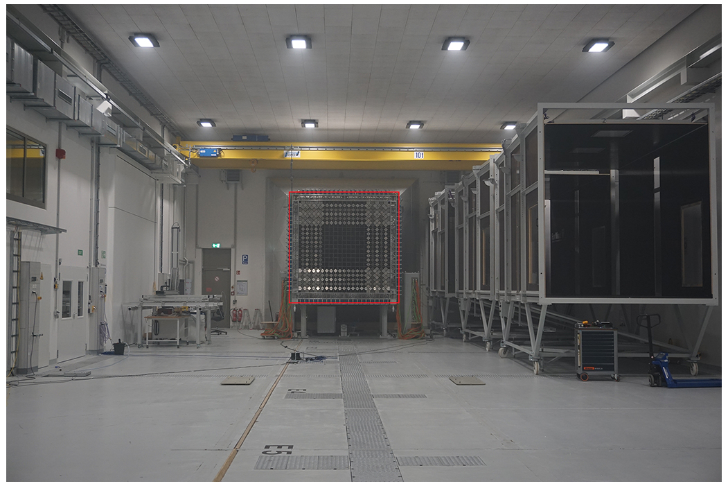
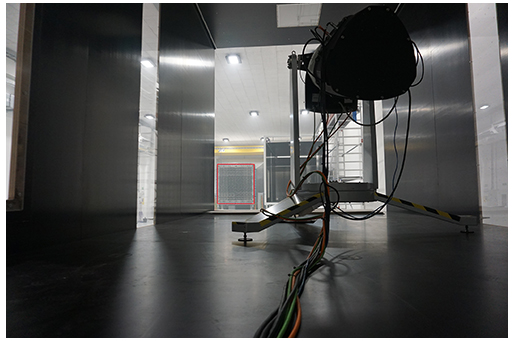
Five 6 m long test sections are available in the wind tunnel to build a closed measurement section. For the present campaign, all test sections are placed near the walls of the wind tunnel, and two of them are used as measurement platforms for the lidars, as illustrated by Fig. 2. In both Figs. 1 and 2, a red frame is drawn to indicate the nozzle with the active grid.

2.2 The short-range WindScanner

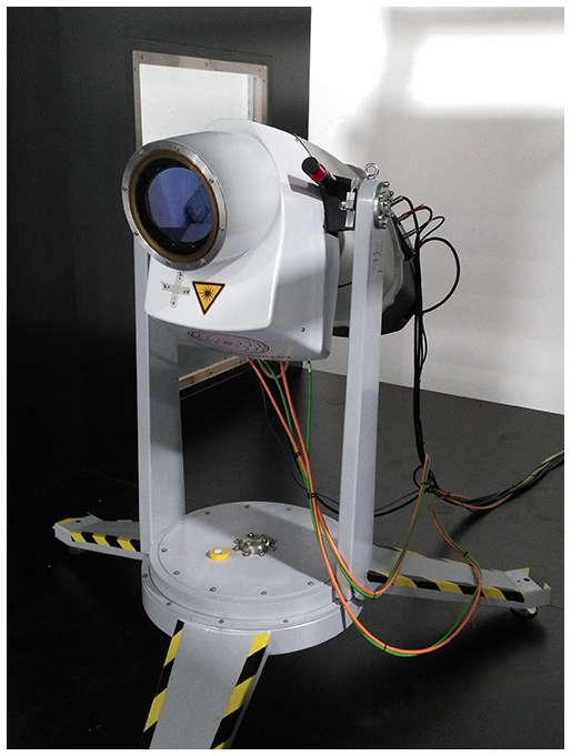
The lidars used for the measurements are two identical continuous-wave short-range WindScanners with a 6 in. aperture (Mikkelsen, 2014; Mikkelsen et al., 2017) developed and manufactured by the Technical University of Denmark (see Fig. 3). The wind speed measured by the WindScanner is based on coherent detection, which is an absolute measurement technique and determined solely by the laser's wavelength and the Doppler shift in hertz. The latter is defined as the difference between the backscattered and emitted laser frequency. As opposed to hot-wire anemometers, Doppler wind lidars do not need calibration. A recent paper by Pedersen and Courtney (2021) has shown that the WindScanner measured wind speeds are detectable with less than 0.1 % absolute uncertainty. The WindScanners set their measurement point by adjusting their focus setting of the telescopes. By changing the metal rods that attach the focus stages to the lens, different focus ranges, hence different scan regimes, can be achieved. The short-range mode allows the lidars to scan and measure at distances between 20 and 300 m, whereas the extra short-range mode, used for the measurement campaign described in this paper, limits the focus range setting to an interval between 12 and 37 m. An important aspect of this reduction in focus length is the corresponding smaller probe length (see Sect. 3.1). Both features are beneficial for wind tunnel measurements.

Figure 3 One of the two short-range WindScanners in the wind tunnel.

The two WindScanners are temporally synchronised at a fixed sampling rate of 451.7 Hz. Because the lidars have a steerable scan head that allows the focused beam to be steered into pointing directions within a cone with a 120^∘ opening angle, they are able to scan along any user-defined trajectory. The pointing accuracy of the two lidars for a fixed staring mode measurement was determined to be below 1 cm for the wind tunnel measurement campaign described here, which was guaranteed by a precise measurement setup geometry and a manual confirmation and adjustment of the focus point of both WindScanners. In order to maintain a sufficient number of aerosols in the wind tunnel to reflect the laser beam, seeding with di-ethyl-hexyl-sebacate (DEHS) was applied every few hours with a PALAS AGF 10.0 liquid nebuliser at the back of the wind tunnel, using the closed return wind tunnel itself for circulation. DEHS has a density of 0.91 g cm⁻³ and a mean particle diameter of 0.5 µm. The aerosol concentration was not confirmed by measurement; however, the quality of the WindScanners' backscatter signal was used as an indirect indicator.

2.3 The hot-wire anemometer

The hot-wire anemometer system used as reference for the wind tunnel measurement campaign consisted of a 54N80 MultiChannel CTA system in combination with a MiniCTA hot-wire probe, both acquired from the manufacturer Dantec Dynamics. The sensor is a basic, one-dimensional hot-wire probe with a wire thickness of 5 µm. It was mounted on a structure with an extended rod and aligned with the mean flow direction, i.e. the x direction, of the wind tunnel. It was calibrated manually every day, before and after the measurement, whilst taking into account a temperature correction. Figure 4 shows the hot-wire probe installation in the wind tunnel, together with the manually adjusted focus points of each respective WindScanner laser beam, visualised by an infrared detector card.

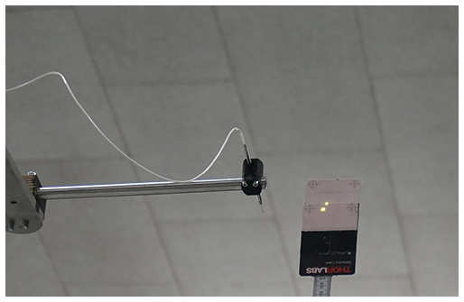
Figure 4 Setup of the hot-wire system next to the adjusted focus points of the WindScanners' laser beams.

2.4 The experimental setup

For an optimal setup of the WindScanner system in the wind tunnel, three important aspects have to be considered:

1. For the largest possible measurement domain coverage within the wind tunnel, with particular interest in the region directly in front of the active grid, and taking into account the minimum focus distance of 12 m, the WindScanners have to be placed as far downstream in the wind tunnel as possible. This also eliminates the obstruction of the flow by the lidars.

2. In order to accurately calculate a two-dimensional wind speed vector, there has to be a favourable opening angle between the beams of the WindScanners (Stawiarski et al., 2013), preferably larger than 30^∘. This means that the transverse distance between the WindScanners has to be maximised.

3. The lidars should measure with a near-zero elevation angle to avoid disturbance by the vertical wind speed component of the turbulent flow.

Although these three aspects cannot be satisfied in an optimal way simultaneously, an acceptable compromise between them is sketched in Fig. 5. The flow enters the measurement section from the left, where the active grid is positioned at the wind tunnel nozzle. WindScanners 1 and 2 are installed at distances of 27.48 and 27.32 m downstream of the nozzle, respectively. Therefore they can cover the region between the active grid and approximately x=15.5 m downstream. The lidars are installed at maximum transverse distance, inside the empty test sections that were parked at the back end of the wind tunnel, such that their separation along the y axis has the largest possible value of 9.7 m. The hot-wire probe (see Fig. 4) was installed at the position indicated in Table 1. It was calibrated twice every day, both at the start and at the end of the measurement. The lidars were focused at a point in space 7 cm away from the hot wire in the positive y direction, to avoid any mutual interference between the sensors (see Fig. 4). The opening angle between the lidars' laser beams for this point is 28.4^∘, which is acceptable for a two-dimensional wind speed reconstruction (Stawiarski et al., 2013). The temporal synchronisation between the WindScanners and the hot wire was established by performing a cross-correlation between the smoothed time series at a 451.7 Hz sampling rate.

Figure 5 Schematic measurement setup of the two WindScanner lidars and the hot wire in the wind tunnel.

Table 1 Coordinates relevant to the experimental setup.

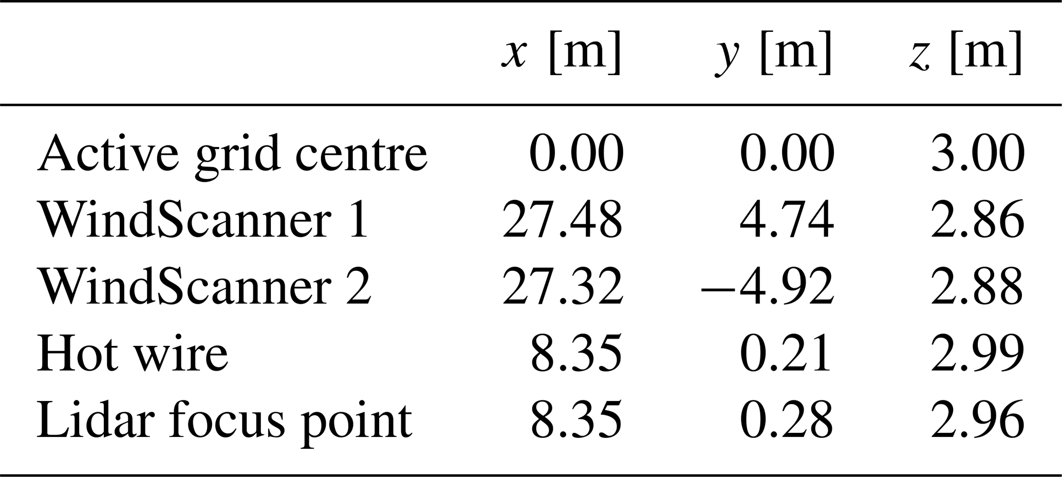
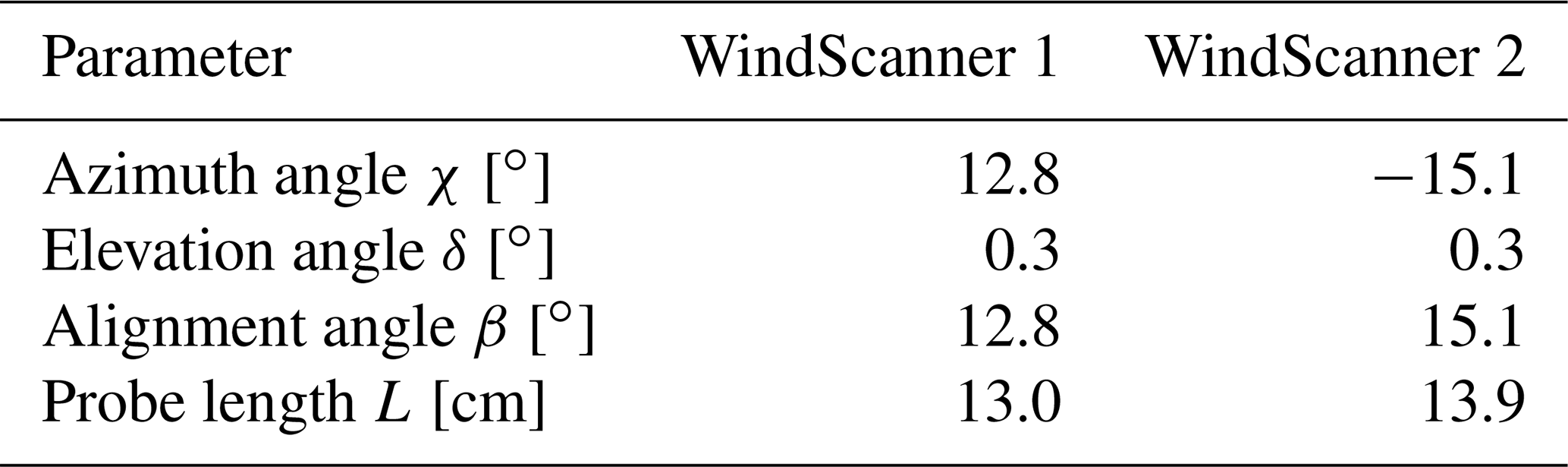
Table 2 Setup parameters describing the WindScanner staring mode scan.

3 Methodology, part II: the physical models

This section introduces the theory used to physically describe and model the lidar measurement principle. A more in-depth description of lidar theory is provided by van Dooren (2021).

3.1 The lidar measurement principle

One of the most important properties of a coherent detection wind lidar is that the measurement point is not an infinitesimal point in space but a probe volume, which is usually a thin cylinder with a radius of less than a millimetre at short ranges and a length in the order of centimetres or metres, depending on the focus distance. In comparison, a hot wire usually has a wire length of a few millimetres. A simple and commonly used physical model for the probe length averaging effect of a CW-lidar measurement comprises a low-pass filter with the shape of a Lorentzian function (Angelou et al., 2012; Slinger and Harris, 2012). In the following, this model is implemented and compared with the actual measurement. This is relevant for the analysis of the measurements in both the wave number space and the frequency domain.

The Lorentzian weighting function is represented by Eq. (1) (Sjöholm et al., 2009):

$$\begin{array}{}\text{(1)}& F={\displaystyle \frac{\mathrm{1}}{\mathit{\pi }}}{\displaystyle \frac{\frac{\mathrm{1}}{\mathrm{2}}L}{{\left(\frac{\mathrm{1}}{\mathrm{2}}L\right)}^{\mathrm{2}}+{\left(s-d_{\mathrm{f}}\right)}^{\mathrm{2}}}},\end{array}$$

where F is the normalised intensity of transmitted laser power along the line-of-sight direction coordinate s, resembling the distance from the lens, d_f is the focus distance and L is the probe length of the WindScanner, defined for CW lidar as the full width at half maximum of the Lorentzian intensity profile symmetrically centred about its focus point, by Eq. (2):

$$\begin{array}{}\text{(2)}& L=\mathrm{2}{\displaystyle \frac{\mathit{\lambda }{d}_{\mathrm{f}}^{\mathrm{2}}}{\mathit{\pi }{a}^{\mathrm{2}}}},\end{array}$$

where λ is the laser wavelength of 1.55 µm, and a is the effective radius of 56 mm of the lidar's 6 in. aperture telescope used for emitting and receiving the laser signal. As the backscattered radiation is proportional to the focused laser beam's power intensity, most of the laser light will be reflected by aerosols in the probe volume; however, a smaller backscatter contribution from outside these bounds is unavoidable.

For the aforementioned extra short-range focus distance range, the probe length varies between 4.5 and 43.1 cm. A plot indicating the probe length for the entire focus distance envelope can be consulted in Fig. 6.

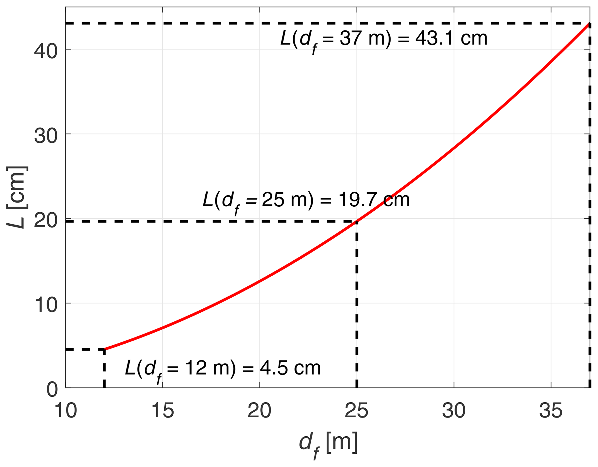
Figure 6 Plot of the theoretical probe length L of the 6 in. aperture WindScanner for the applied focus distance d_f ranging from 12 to 37 m.

A single Doppler wind lidar can only measure a one-dimensional component of the wind speed, i.e. the projection of the full three-dimensional wind velocity vector onto its line-of-sight direction, indicated by Eq. (3):

$$\begin{array}{}\text{(3)}& v_{\mathrm{LOS}}=\left[\begin{array}{l}\cos \left(\mathit{\chi }\right)\cos \left(\mathit{\delta }\right)\\ \sin \left(\mathit{\chi }\right)\cos \left(\mathit{\delta }\right)\\ \sin \left(\mathit{\delta }\right)\end{array}\right]\cdot \left[\begin{array}{l}u\\ v\\ w\end{array}\right],\end{array}$$

where v_LOS is the line-of-sight wind speed measured by the lidar, χ and δ are the azimuth and elevation angles of the line-of-sight direction, respectively, and u, v and w are the wind speed components in x, y and z direction, respectively.

Assuming the vertical wind speed w to be zero, a two-dimensional horizontal wind vector is calculated from two linearly independent measurements from different lidars through Eq. (4):

$$\begin{array}{}\text{(4)}& \left[\begin{array}{lr}\cos \left({\mathit{\chi }}_{\mathrm{1}}\right)\cos \left({\mathit{\delta }}_{\mathrm{1}}\right)& \sin \left({\mathit{\chi }}_{\mathrm{1}}\right)\cos \left({\mathit{\delta }}_{\mathrm{1}}\right)\\ \cos \left({\mathit{\chi }}_{\mathrm{2}}\right)\cos \left({\mathit{\delta }}_{\mathrm{2}}\right)& \sin \left({\mathit{\chi }}_{\mathrm{2}}\right)\cos \left({\mathit{\delta }}_{\mathrm{2}}\right)\end{array}\right]\left[\begin{array}{l}u\\ v\end{array}\right]=\left[\begin{array}{l}{v}_{{\mathrm{LOS}}_{\mathrm{1}}}\\ v_{{\mathrm{LOS}}_{\mathrm{2}}}\end{array}\right],\end{array}$$

where the indices 1 and 2 refer to the respective lidar. The wind speed vector [u v]^T can be calculated as the solution to this linear system, which we will refer to as dual-Doppler reconstruction.

Apart from the dual-Doppler reconstruction, for which two lidars are needed, it is also possible to calculate each single-lidar wind speed estimate. To be able to compare the performance of the two WindScanners, most of the results in this paper are based on one-dimensional projection measurements, calculated by Eq. (5):

$$\begin{array}{}\text{(5)}& u_{\mathrm{p}}={\displaystyle \frac{v_{\mathrm{LOS}}}{\cos \left(\mathit{\chi }\right)\cos \left(\mathit{\delta }\right)}},\end{array}$$

where u_p is the projected u component, under the assumption that v and w, weighted by their respective sine and cosine components in Eq. (3), are negligible with respect to u_p.

3.2 Lidar spectral modelling

For a deeper understanding of the measurement principle of CW lidar, it can be further investigated in the frequency domain (Angelou et al., 2012; Held and Mann, 2018). Our aim is to define a model for the spectral density function of a lidar measurement, encompassing a theoretical probe volume averaging filter and a white noise term. The spatial filter which the lidar's probe volume exerts on the turbulence along its line-of-sight direction is described by the aforementioned Lorentzian function in Eq. (1). This probe volume acts as a low-pass filter that reduces the spectral energy content of the turbulent eddies with wavelengths smaller than the axial extent of the probe volume; however, the spectrum measured by the lidar usually still shows a significant energy content in the spectral range above that cut-off frequency. The lidar's measured spectrum may be artificially increased for higher frequencies due to random noise on the measurements, associated with low signal-to-noise levels, which depend on the aerosol density in the wind tunnel. According to our findings, the lidar's measured spectrum tends towards a horizontal curve at the highest frequency range, which is an indication for the noise being white. This assumption is in agreement with previous research (Sjöholm et al., 2009; Angelou et al., 2012). Therefore, the model also includes a flat spectrum white noise term.

The proposed model in the time domain is given by Eq. (6):

$$\begin{array}{}\text{(6)}& {\widehat{v}}_{\mathrm{LOS}}={\displaystyle \frac{\mathrm{1}}{\mathit{\pi }}}\underset{-\mathrm{\infty }}{\overset{\mathrm{\infty }}{\int }}{\displaystyle \frac{\frac{\mathrm{1}}{\mathrm{2}}L}{{\left(\frac{\mathrm{1}}{\mathrm{2}}L\right)}^{\mathrm{2}}+{\left(s-d_{\mathrm{f}}\right)}^{\mathrm{2}}}}u\left(s\right)\mathrm{d}s+{\mathit{\sigma }}_{\mathit{\eta }}\mathit{\eta },\end{array}$$

where ${\widehat{v}}_{\mathrm{LOS}}$ is the modelled WindScanner line-of-sight time series, u(s) is the actual wind speed ucos (χ)cos (δ) to which the Lorentzian filter is applied, s is the coordinate along the line-of-sight direction, η is a dimensionless Gaussian noise term with a mean of zero and a standard deviation of 1, and σ_η is the magnitude of the standard deviation (in m s⁻¹) of the noise term. Please note that the estimated ${\widehat{v}}_{\mathrm{LOS}}$ is not meant to closely correlate to the actual v_LOS measurement in the time domain, which is impossible due to the random nature of the modelled noise term. The goal of this approach is to find a time series ${\widehat{v}}_{\mathrm{LOS}}$ with the same features in the frequency domain as v_LOS, by qualitatively comparing the spectral density functions.

A vital assumption for the model in Eq. (6) is that the hot-wire measurements, although also low-pass-filtered but at a much higher frequency, resemble the actual wind speed at the focus point of the lidar. In order to apply the spatial Lorentzian filter to a temporally sampled time series, we apply Taylor's frozen turbulence hypothesis (Taylor, 1938). This relies on the assumption that turbulence is advected through the lidar's probe volume by the mean wind speed without decaying.

In the frequency domain, the effect of the Lorentzian filter can be expressed in terms of the spectral transfer function T(β,f) in Eq. (7) (Kristensen et al., 2011):

$$\begin{array}{}\text{(7)}& \begin{array}{rl}T\left(\mathit{\beta },f\right)& ={\displaystyle \frac{\mathrm{11}}{\mathrm{9}\sqrt{\mathit{\pi }}}}{\displaystyle \frac{\mathrm{\Gamma }(\mathrm{1}/\mathrm{3})}{\mathrm{\Gamma }(\mathrm{5}/\mathrm{6})}}{\sin }^{\mathrm{5}/\mathrm{3}}\left(\mathit{\beta }\right){\left(\mathit{\pi }{\displaystyle \frac{f}{f_{\mathrm{c}}}}\right)}^{-\mathrm{1}}\\ & +{\displaystyle \frac{\mathrm{1}}{\mathrm{2}}}\left(\mathrm{7}\cos \left(\mathrm{2}\mathit{\beta }\right)-\mathrm{5}\right)e^{-\mathit{\pi }\frac{f}{f_{\mathrm{c}}}},\end{array}\end{array}$$

where the angle β denotes the angle between the lidar's line-of-sight direction and the mean flow direction, f is frequency, f_c is the probe length cut-off frequency to be defined in Sect. 4.1 and Γ is the gamma function. This function can be applied as a multiplier on an un-truncated turbulent inertial sub-range spectrum with an exponent equal to $-\mathrm{5}/\mathrm{3}$ according to Kolmogorov (1941) of the wind component in the mean wind direction, in order to resemble the spectrum of a time series measured by the lidar, pointed at the mean wind direction under an angle β that has passed through a Lorentzian filter. The full derivation of Eq. (7) is provided in Appendix A.

Since the mean wind tunnel flow is aligned with the x direction, we can express the angle β as a combination of both azimuth and elevation angles of the WindScanners, as stated by Eq. (8):

$$\begin{array}{}\text{(8)}& \mathit{\beta }=\arccos \left(\cos \right(\mathit{\chi }\left)\cos \right(\mathit{\delta }\left)\right).\end{array}$$

In the case of zero misalignment between the lidar line-of-sight direction and the mean flow direction, the spectral transfer function T(f) reduces to

$$\begin{array}{}\text{(9)}& T\left(f\right)=e^{-\mathit{\pi }\frac{f}{f_{\mathrm{c}}}}.\end{array}$$

We are now able to model the observed spectral density function of a CW lidar measuring turbulence within the inertial sub-range, simply by multiplying the observed hot-wire spectrum, which represents the un-filtered inertial sub-range spectrum of the turbulence component aligned with the mean wind direction, by the lidar transfer function T(β,f) and subsequently adding a white noise term S_η(f) to it, as Eq. (10) illustrates:

$$\begin{array}{}\text{(10)}& S\left(f\right)=T(\mathit{\beta },f)S_u\left(f\right)+{\mathit{\sigma }}_{\mathit{\eta }}^{\mathrm{2}}{S}_{\mathit{\eta }}\left(f\right),\end{array}$$

where S(f) is the modelled lidar spectrum, S_u(f) is the hot-wire spectrum and S_η(f) is the spectrum of white noise with a mean of zero and a standard deviation of 1, which has to be scaled with the variance ${\mathit{\sigma }}_{\mathit{\eta }}^{\mathrm{2}}$ for each specific case. White noise (Kuo, 1996) has the property that its power density spectrum S_η(f) shows the same energy content at each given frequency, which lets us maintain a low complexity of the model. Although the spectral density function is proportional to the square of a Fourier transform of the measured time series, the spectral densities of both the filtered hot-wire time series and the white noise can be joined by a simple addition, since they are assumed to be uncorrelated.

To complete the model, the standard deviation of the noise σ_η has to be expressed. We hypothesised based on our findings that this variable is connected to the energy dissipation rate ε of the classic Kolmogorov spectrum, the mean wind speed μ_u or a combination of both. The dependency of σ_η on the standard deviation of the mean σ_u was also investigated but proved to be unconvincing. Throughout the wind tunnel measurement campaign, the ambient temperature was measured to be in the range between 17.8 and 19.1 ^∘C and confirmed to show no significant correlation with the value of σ_η either. Based on empirical analysis, by investigating the linear dependency of σ_η on various combinations of the aforementioned variables, with respect to manually tuned values of σ_η for seven cases, the following model is suggested:

$$\begin{array}{}\text{(11)}& {\widehat{\mathit{\sigma }}}_{\mathit{\eta }}=\sqrt{{\displaystyle \frac{{\mathit{\mu }}_u\mathit{\epsilon }}{C}}},\end{array}$$

where C is a constant of 563 m s⁻² found by performing a linear fit between calculated and manually tuned σ_η values, and ε is the energy dissipation rate calculated by fitting the theoretical Kolmogorov spectrum adapted from Wang et al. (2020) to the hot-wire spectrum in the inertial sub-range. Appendix B elaborates on the procedure used to determine the relationship expressed in Eq. (11). The Kolmogorov spectrum for the longitudinal wind speed component in the inertial sub-range is modelled by Eq. (12):

$$\begin{array}{}\text{(12)}& S\left(f\right)=\mathrm{0.5}{\mathit{\epsilon }}^{\frac{\mathrm{2}}{\mathrm{3}}}{\left({\displaystyle \frac{\mathrm{2}\mathit{\pi }f}{{\mathit{\mu }}_u}}\right)}^{-\frac{\mathrm{5}}{\mathrm{3}}}.\end{array}$$

4 Results and discussion

The Results and discussion section is divided into three parts: first the WindScanner lidar measurements are validated by comparing them to hot-wire anemometer measurements. Afterwards, the lidars' ability to measure turbulent gusts generated by the active grid in the wind tunnel is analysed. Finally, the power spectral density model for CW lidar is evaluated.

4.1 Comparison between WindScanner and hot-wire anemometer measurements

As an evaluation of the equipment and the measurement setup, a comparison of the WindScanner lidar measurements to those obtained from a hot-wire anemometer was carried out for instantaneously sampled time series on a 10 min basis, for cases of both low and high turbulence intensity. The WindScanner and hot-wire anemometer measurements were sampled at 451.7 and 1000 Hz, respectively. The latter was downsampled to the lidar sampling rate by means of linear interpolation.

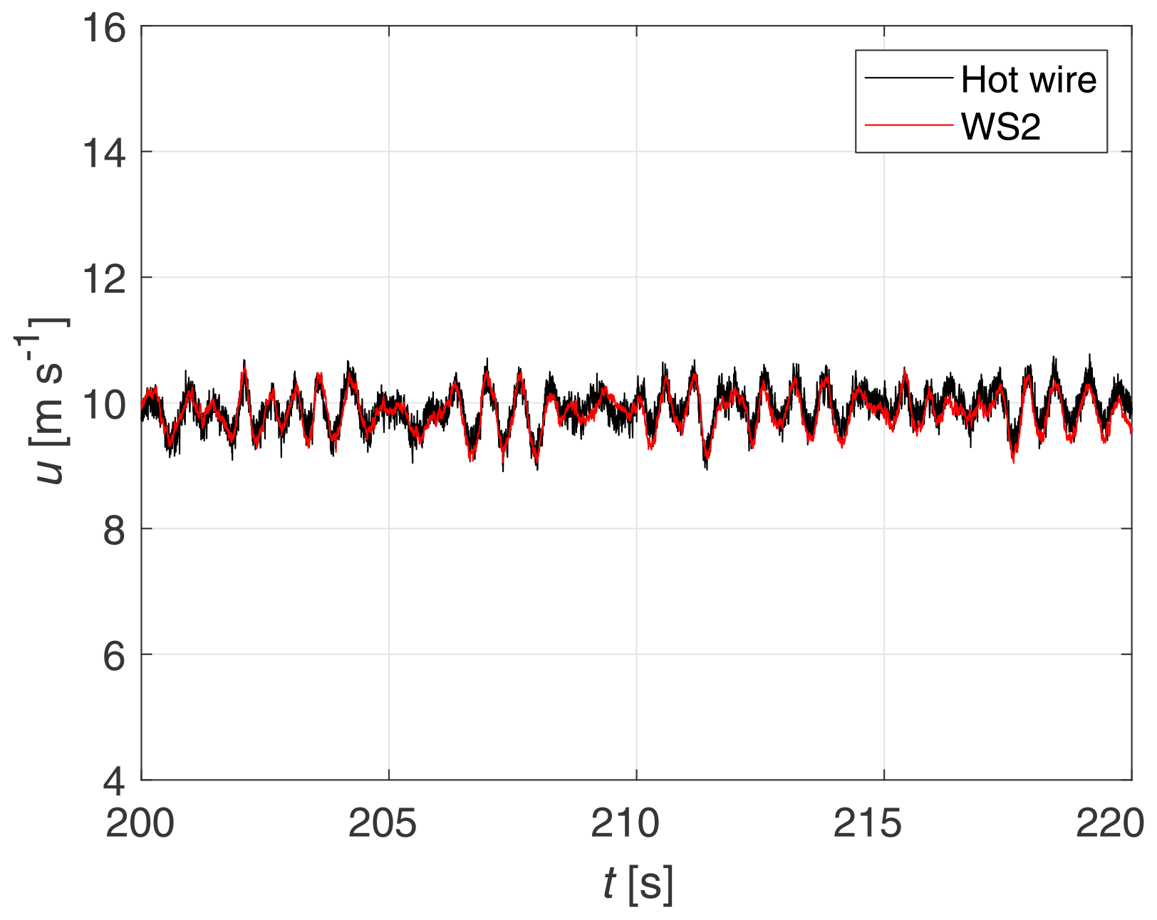
Figure 7 Snapshot of the 10 min time series measured by WindScanner 2 and the hot-wire anemometer for a turbulence intensity of 3 % (Case 1a).

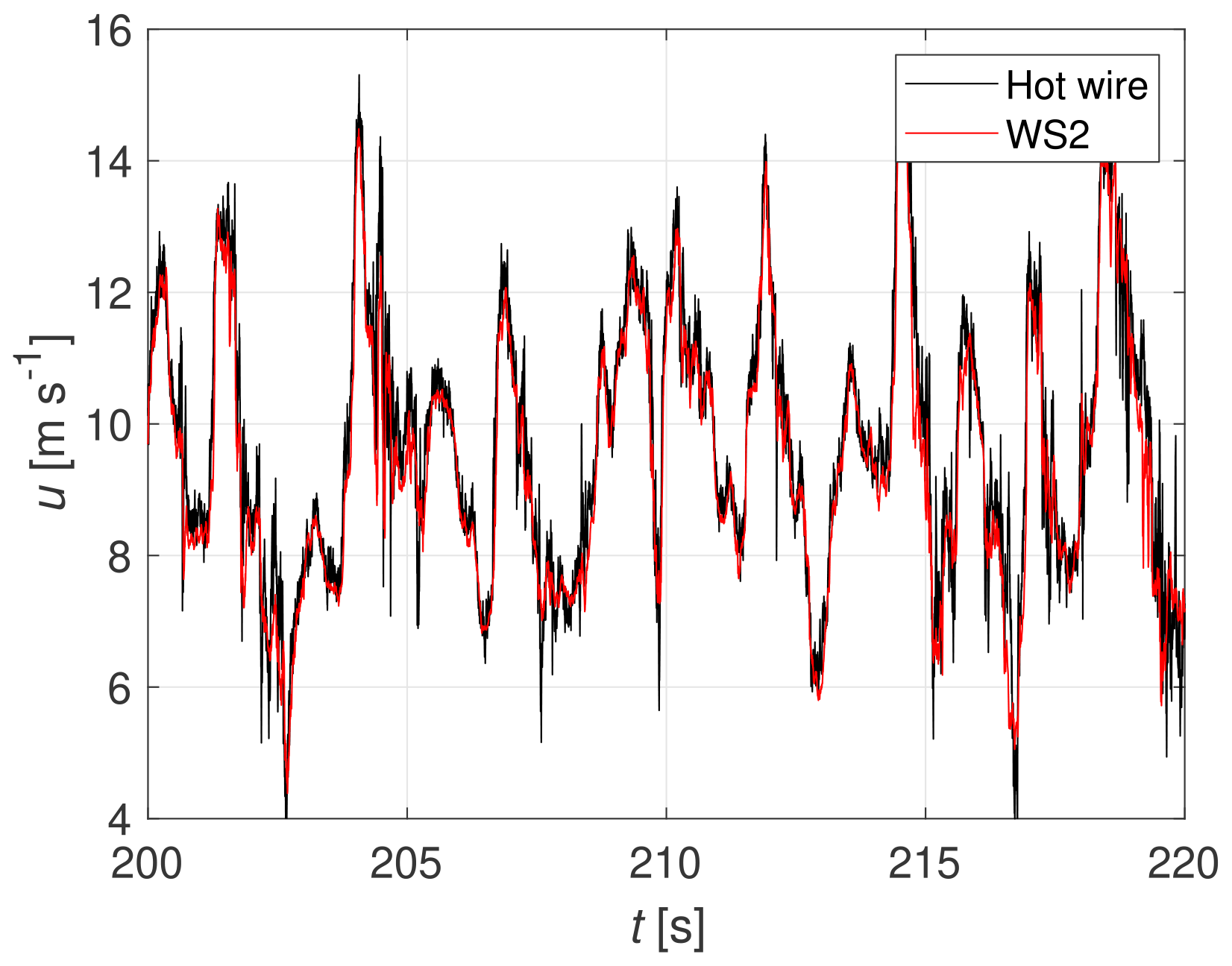
Figure 8 Snapshot of the 10 min time series measured by WindScanner 2 and the hot-wire anemometer for a turbulence intensity of 22 % (Case 1b).

Figures 7 and 8 show a 20 s snapshot of the 10 min time series measured by the hot wire and WindScanner 2, for two different turbulent conditions: Cases 1a and 1b, respectively. The black line resembles the wind speed measured by the hot wire, which is aligned with the x direction to measure the u component. The red line represents the projected u_p component of the wind speed, calculated by applying Eq. (5) to the measured line-of-sight wind speed of WindScanner 2. Case 1a with TI = 3 % was established by a fully opened active grid, effectively operating in a passive mode. For Case 1b with TI = 22 % the active grid ran a turbulent protocol based on the approach by Neuhaus et al. (2020). An overview of the corresponding statistics is provided in Table 3, where μ_u and σ_u are the mean and the standard deviation of the wind speed component u, respectively. The aforementioned turbulence intensity TI is defined on the basis of those statistics by Eq. (13):

$$\begin{array}{}\text{(13)}& \mathrm{TI}={\displaystyle \frac{{\mathit{\sigma }}_u}{{\mathit{\mu }}_u}}.\end{array}$$

By looking at the time series themselves, some differences in the turbulence behaviour can already be observed. For Case 1a there is a visible dominating frequency, with additional superimposed small-scale fluctuations. In Case 1b we do not identify such a distinct dominating frequency, but instead see a superposition of relatively large-scale structures and some small-scale fluctuations. This difference will be addressed in the following part of the subsection.

Table 3 Statistics of the 10 min hot-wire and WindScanner time series of the u component of the wind.

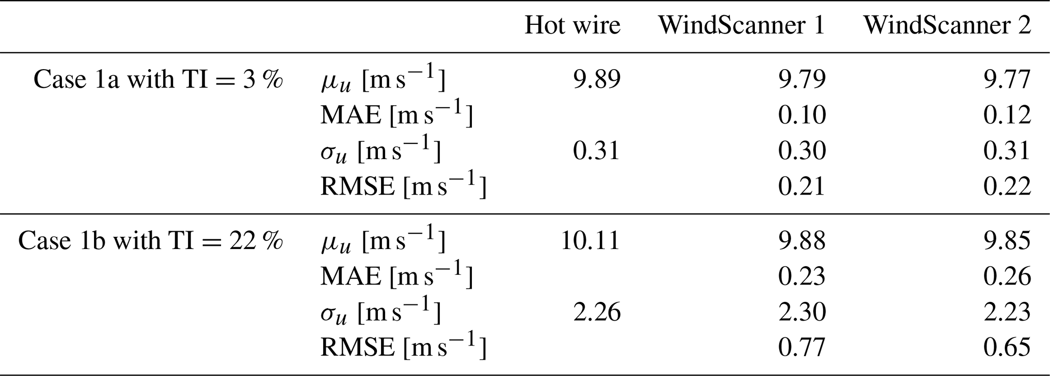
The values of the mean u component in Table 3 indicate that the WindScanners have a mean average error (MAE) relative to the hot-wire measurement of 0.10 and 0.12 m s⁻¹ for Case 1a, respectively, and 0.23 and 0.26 m s⁻¹ for Case 1b, respectively. This effect might be related to the measurement volume, which has a finite probe length L and is not aligned with the x direction. Even though the wind speed has been corrected for the scanning angles χ and δ by means of Eq. (5), the way the probe lengths of about 13.0 and 13.9 cm respectively (see Table 2) cross through the measurement point causes an averaging of the u component with contributions from outside the desired point. The bias may also be related to the uncertainty of the hot-wire calibration, given that the WindScanners proved to have an uncertainty below 0.1 % (Pedersen and Courtney, 2021). In contrast to the wind speed mean, only minor differences can be observed between the measured standard deviations. The root-mean-square error (RMSE) of WindScanner 1 and 2 with respect to the hot wire is 0.21 and 0.22 m s⁻¹ for Case 1a, respectively, and 0.77 and 0.65 m s⁻¹ for Case 1b, respectively. Case 1b shows a higher value as well as a larger difference between the two WindScanners.

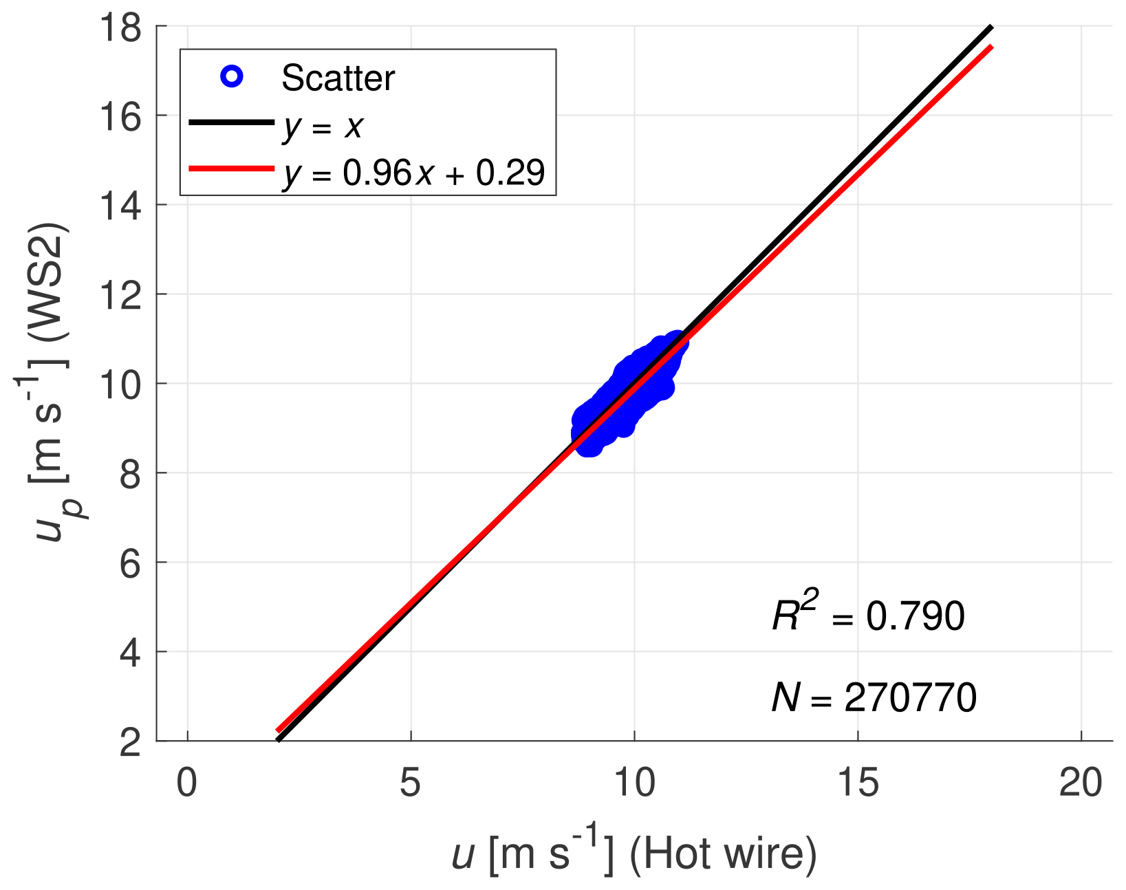
Figure 9 Correlation between WindScanner 2 and the hot-wire anemometer for a turbulence intensity of 3 % (Case 1a).

Figure 10 Correlation between WindScanner 2 and the hot-wire anemometer for a turbulence intensity of 22 % (Case 1b).

Figures 9 and 10 show the linear regression plots of the correlation of the full time series corresponding to Figs. 7 and 8, respectively. To eliminate the small scales that cannot be resolved by the WindScanners from this evaluation, a moving average with a window size of 20 samples was applied to both the hot wire and the lidar time series. For Cases 1a and 1b, the goodness-of-fit coefficients R² are 0.790 and 0.957, respectively. It seems counter-intuitive that the case with higher turbulence is measured more accurately by the WindScanner. This might be a numerical artefact resulting from the significantly different wind speed range. However, it should be kept in mind that the spectral characteristics of both time series strongly differ. An alternative explanation to the R² difference will be given in the following after performing a spectral analysis.

Figures 11 and 12 display the spectral density functions of the wind speed measurements corresponding to Figs. 9 and 10, respectively. To create the spectra, and all other spectra in the following, we performed Hann smoothing with N=10 non-overlapping Hann windows. Because of the lidar measurement principle, turbulent structures with a length scale smaller than the probe length are partly filtered out. Assuming again the Taylor's frozen turbulence hypothesis and the Nyquist criterion, the probe length cut-off frequency f_c corresponding to the smallest turbulence scales that can be measured relatively un-truncated by the lidars is estimated with Eq. (14):

$$\begin{array}{}\text{(14)}& f_{\mathrm{c}}={\displaystyle \frac{\mathrm{1}}{\mathrm{2}}}{\displaystyle \frac{u_{\mathrm{\infty }}}{L}},\end{array}$$

where L is the probe length, and u_∞ is the free-stream wind speed in the wind tunnel, assumed to be represented by the average of the wind speed time series measured by the hot-wire anemometer. For Case 1a the probe length of WindScanner 2 is 13.9 cm, and the mean wind speed is 9.89 m s⁻¹, leading to a probe length cut-off frequency of 35.6 Hz. For Case 1b, the mean wind speed increased to 10.11 m s⁻¹, leading to a slightly higher cut-off frequency of 36.4 Hz. These values are indicated in Figs. 11 and 12 with a magenta line. The variable f_cc will be defined later in Sect. 4.2.

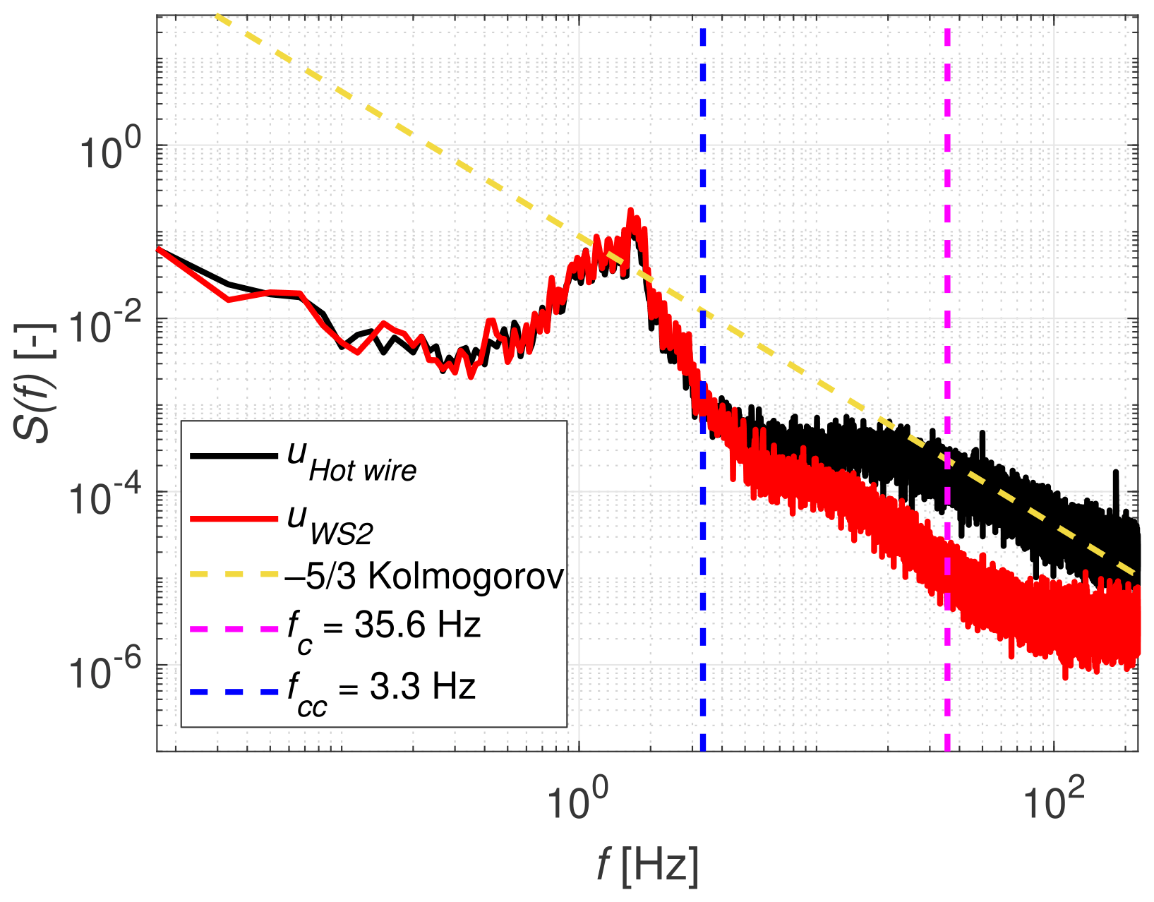
Figure 11 Spectrum of WindScanner 2 and the hot-wire anemometer for a turbulence intensity of 3 % (Case 1a).

Figure 12 Spectrum of WindScanner 2 and the hot-wire anemometer for a turbulence intensity of 22 % (Case 1b).

By means of these spectra, we can now readdress the observation regarding the time series in Figs. 7 and 8 and the difference in the goodness-of-fit coefficients of the linear regression plots in Figs. 9 and 10. The spectrum for the low turbulence case shows a clear signature of high energy content around 1.65 Hz, which confirms our observation of a dominating frequency based on visual inspection of the time series. This frequency has been addressed as a common phenomenon in open-duct wind tunnels before (Wickern et al., 2000) and can be explained by vortex shedding occurring around the nozzle. This phenomenon causes a pulsating pressure wave, leaving a characteristic fluctuation pattern in the wind speed time series in Fig. 7. According to Wickern et al. (2000), the vortex shedding frequency of an open duct can be calculated by Eq. (15):

$$\begin{array}{}\text{(15)}& f_{\mathrm{vs}}=St{\displaystyle \frac{u_{\mathrm{\infty }}}{D}},\end{array}$$

where f_vs is the vortex shedding frequency, St is the Strouhal number and D is the diameter of the nozzle, which is equated here with the square width W of the nozzle. Solving this equation for our known parameters u_∞=9.89 m s⁻¹ and W=3 m, a Strouhal number St=0.5 is found, which is in accordance with the findings by Ahuja et al. (1997) and Wickern et al. (2000).

The high TI spectrum does not show this peak but has a significantly higher energy content broadly distributed over the lower frequency region, representing the more dominant presence of longer length scales. This explains why the WindScanners have a better correlation with the hot wire for the high turbulence case, since the CW lidars are much more capable of measuring large-scale structures over small-scale fluctuations. The small scales play a more dominant role in the spectrum of the low TI case, which was confirmed by integrating the spectrum between $\mathrm{0}<f<f_{\mathrm{cc}}$ and $f_{\mathrm{cc}}<f<\mathrm{\infty }$, for both cases respectively, and expressing the ratio of the variance in both ranges. This approach yielded a contribution of the turbulence scales with f>f_cc of 20.4 % and 3.8 % to the total integrated variance, for Case 1a and 1b, respectively.

The visually observed frequencies at which the WindScanner spectra drop from the hot-wire spectra imply a significantly lower limit than the prediction by Eq. (14) according to Taylor's frozen turbulence hypothesis and the Nyquist criterion. Possible reasons for this are the insufficiency of the full width at half maximum metric to characterise the effective probe length and the invalidity of the assumption of isotropic turbulence, combined with the misalignment between the line of sight and the x direction.

4.2 Analysis of WindScanner measurements of turbulent gusts

In order to analyse the WindScanners' ability to measure gusts, we set up an additional five cases, where an identical 10 min gust protocol based on the approach by Neuhaus et al. (2021) was run by the active grid, and only the mean wind speed in the wind tunnel was varied between 2.36 and 11.25 m s⁻¹. However, the varying wind speed naturally affects the coefficient of variation $c_{\mathrm{v}}={\mathit{\sigma }}_u/{\mathit{\mu }}_u$, i.e. between 11.7 % and 16.4%. This is illustrated by Fig. 13, which serves as a summary of the hot-wire statistics for the five investigated cases. This particular active grid protocol was selected for its ability to generate a time series containing structures with varying length scales, providing a suitable test case for the WindScanner measurement. Please note that we opt for the coefficient of variation c_v instead of the turbulence intensity TI here, since the fluctuations introduced by the artificially generated gusts do not comply with the classic definition of TI.

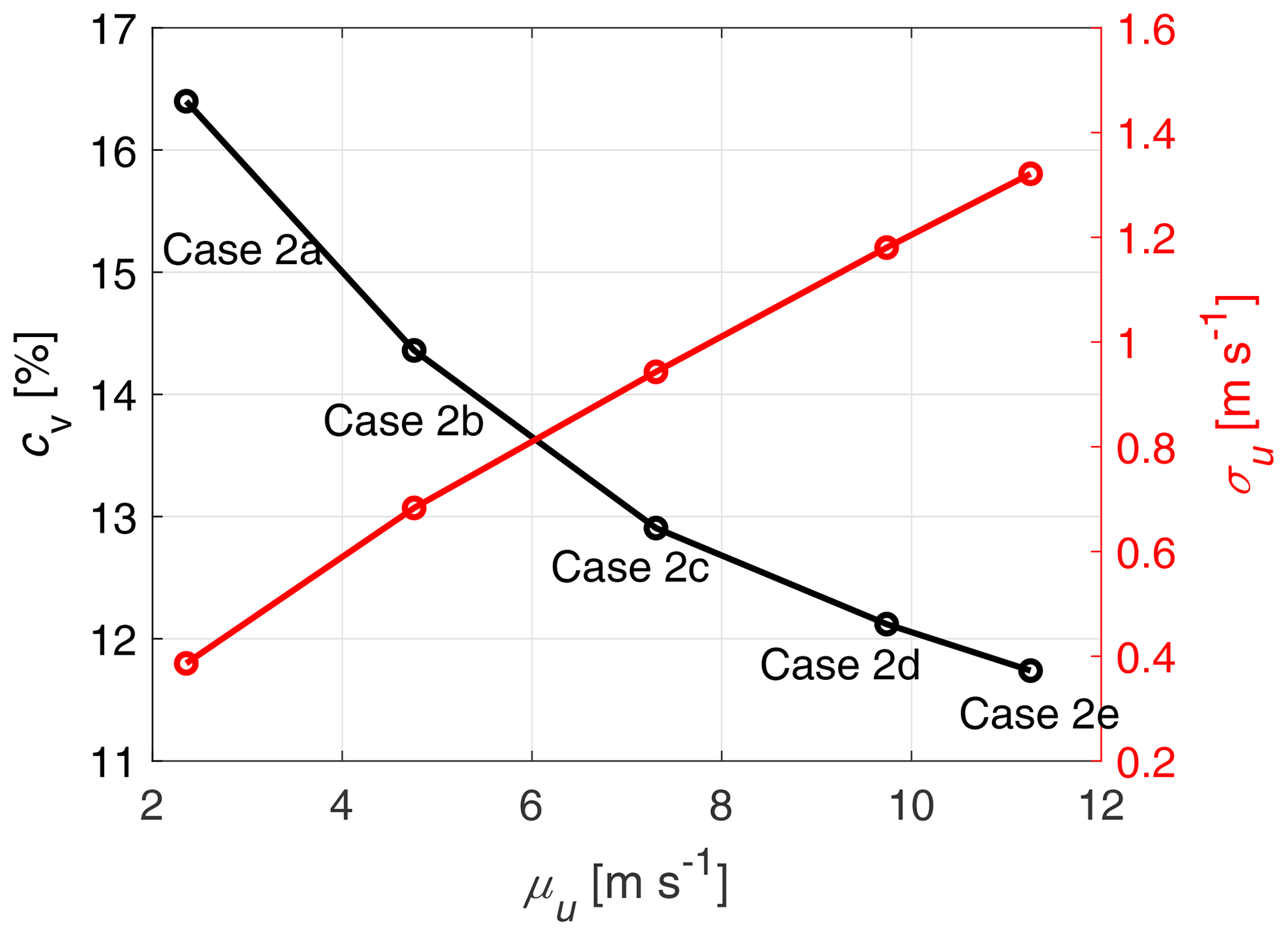
Figure 13 Plot of the standard deviation σ_u and coefficient of variation c_v as a function of the mean wind speed μ_u calculated from the hot-wire time series of each of the five cases 2a–2e.

Even though the hot wire was calibrated twice every day, the post-processing revealed a bias relative to the WindScanner measurements equal to −5.2 % of the mean wind speed for this data. This bias was constant throughout Cases 2a–2e of the measurement campaign, i.e. the measurement of turbulent gusts, but did not occur at all during the validation measurement (Cases 1a and 1b) that was done a few months prior. After careful reassessment of the entire measurement chain, we assumed it was caused by a faulty hot-wire calibration, and therefore we corrected the hot-wire measurements by a factor of 0.948 as a part of the post-processing to yield a satisfactory match between the measurement sensors. This has to be taken into consideration when assessing the results.

For a more comprehensive overview of the statistics measured during each of the five cases, see Table 4. It contains the mean and standard deviation values of the 10 min time series measured by the hot wire, WindScanner 1 and 2, as well as the dual-Doppler reconstructed wind speed.

Table 4 Statistics of the hot-wire and WindScanner time series of the u component of the wind speed.

Figure 14 shows the measured wind speed time series, produced by the active grid running a gust protocol, for Case 2c. The protocol cycles through a series of gusts, facilitating a combination of gusts with varying duration and intensity. This allows the analysis of the performance of the CW lidar for a wide range of turbulence scales. The protocol has a duration of approximately 100 s, which is repeated six times to yield a 10 min time series. Each of the cycles contains 10 distinct gusts. Figure 15 displays three such gusts, which occur between t=200 and t=220 s.

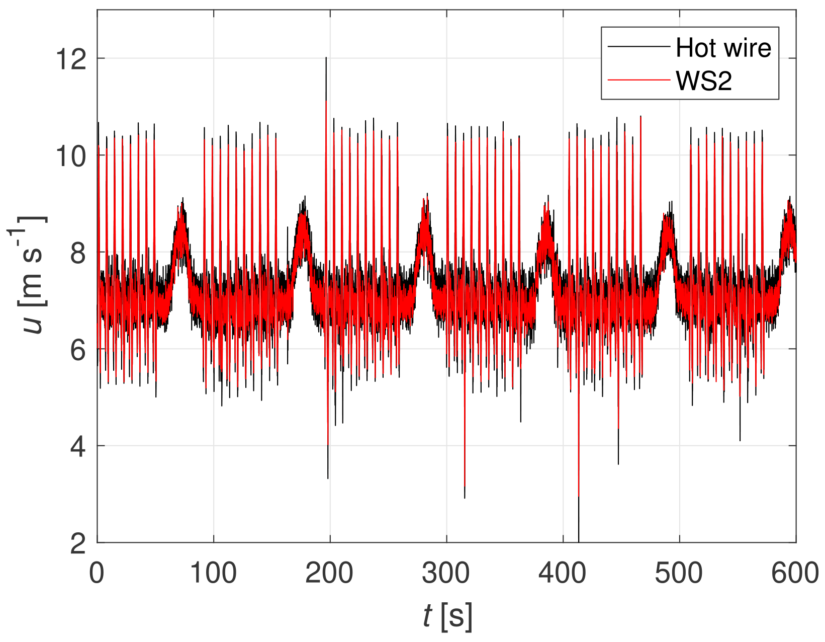
Figure 14 The 10 min time series measured by WindScanner 2 and the hot-wire anemometer for a coefficient of variation of 12.9 % (Case 2c).

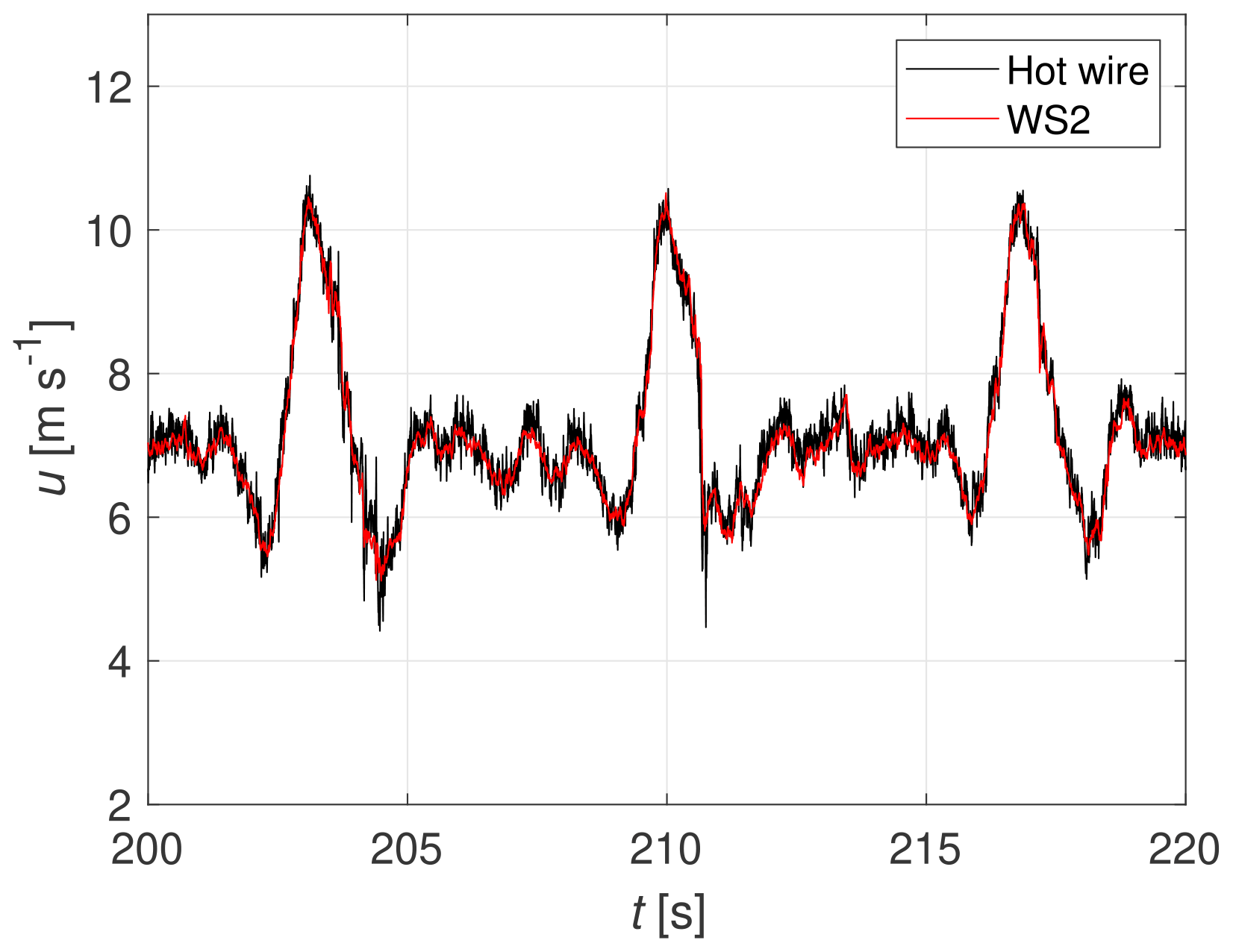
Figure 15 Snapshot of the 10 min time series measured by WindScanner 2 and the hot-wire anemometer for a coefficient of variation of 12.9 % (Case 2c).

In both Figs. 14 and 15, the black line is the wind speed u measured by the hot wire, and the red line resembles the projected u_p component of the wind speed of WindScanner 2. At first glance, it can be seen that the WindScanner measurements have a narrower spread than the hot wire, indicating that the smallest turbulence scales are filtered out in the probe volume.

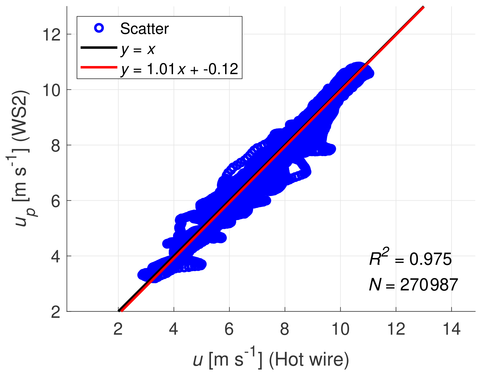
Figure 16 Correlation between WindScanner 2 and the hot-wire anemometer for a coefficient of variation of 12.9 % (Case 2c).

Figure 16 illustrates the correlation between the projected wind speed based on WindScanner 2 and the hot-wire measurement for Case 2c, corresponding to the time series of Fig. 14 with 451.7 Hz sampling rate. As before, a moving average with a window size of 20 samples was applied to the time series. A goodness-of-fit coefficient of R²=0.975 was found, which is similar to the value for Case 1b in Fig. 10. The linear regression curve has a slope of 1.01 and an offset of −0.12 m s⁻¹.

Figure 17 Correlation between WindScanner and hot-wire time series, as a function of coefficient of variation, for both 451.7 Hz (solid lines) and 1 Hz (dashed lines) resolution. HW denotes the hot wire, WS1 and WS2 stand for WindScanner 1 and 2, respectively, and WS resembles the dual-Doppler reconstruction.

To investigate the effect of coefficient of variation on the accuracy of the WindScanner measurement with respect to the hot wire, the correlation for Cases 2a–2e is plotted in Fig. 17. Here all solid lines represent the correlation of the highly resolved 451.7 Hz time series, and the respective dashed lines resemble the correlation between the 1 Hz averaged time series. The 1 Hz averaging was applied to investigate the correlation after further eliminating the small-scale turbulence fluctuations that cannot be fully resolved by the CW lidar.

We see a decreasing trend for the correlation of all sensors with respect to the coefficient of variation. However, for all cases, the goodness-of-fit coefficient R² is higher than 0.9. For both the highly resolved and averaged time series, WindScanner 2 correlates better to the hot wire than WindScanner 1 does. The dual-Doppler reconstruction performance lies closest to the curve for WindScanner 2. The correlation between the two WindScanners is not the highest, even though they are identical devices. This may be attributed to different tolerances in the optical system, most likely related to the prisms and the lens. For all 1 Hz averaged cases, the goodness-of-fit coefficient is above 0.96. The order in which the correlation curves are plotted is the same as for the highly resolved time series, the only exception being the correlation between the two WindScanners.

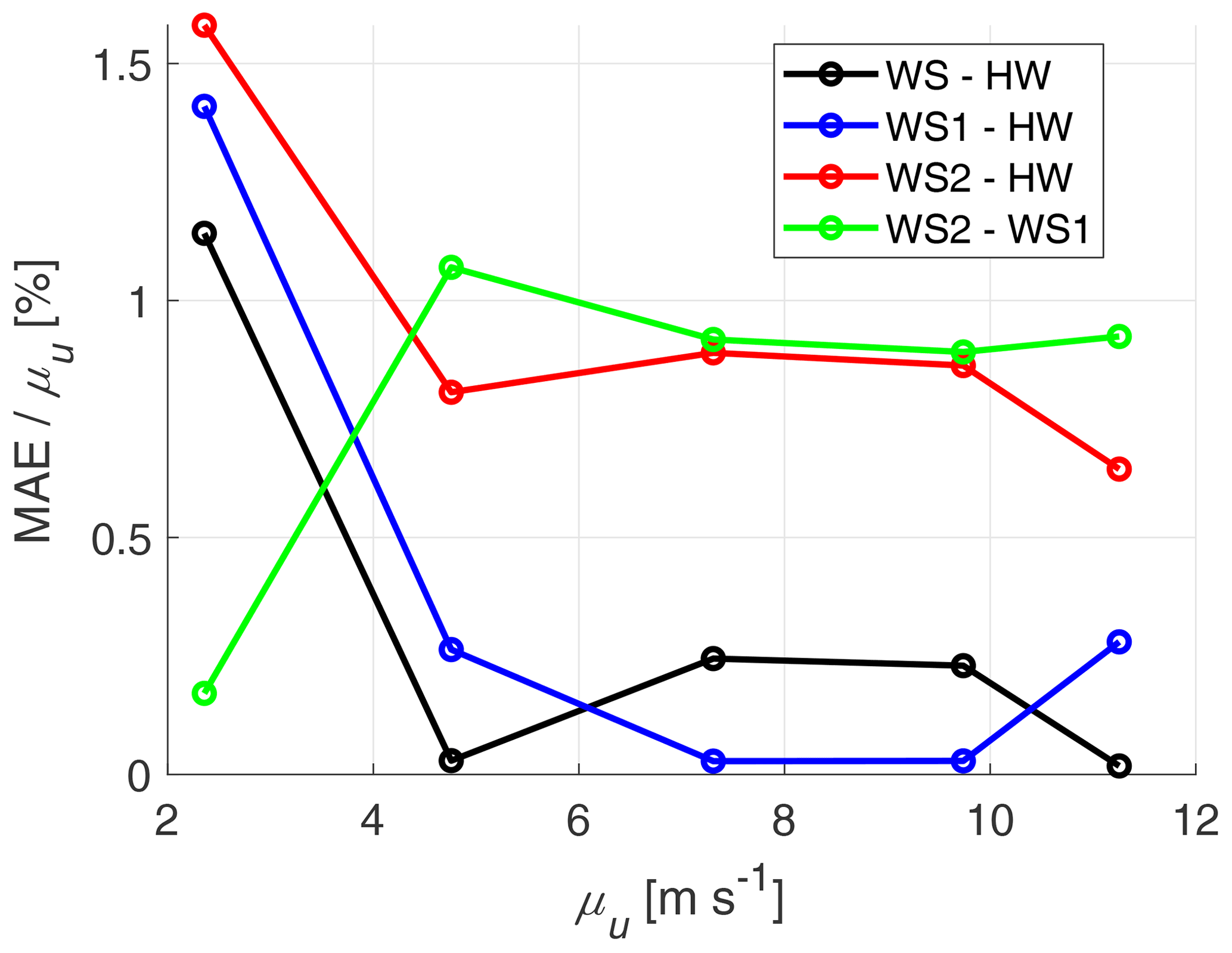
Figure 18 Normalised mean averaged error of the measured wind speed with respect to the hot-wire anemometer for each of the five cases at 451.7 Hz.

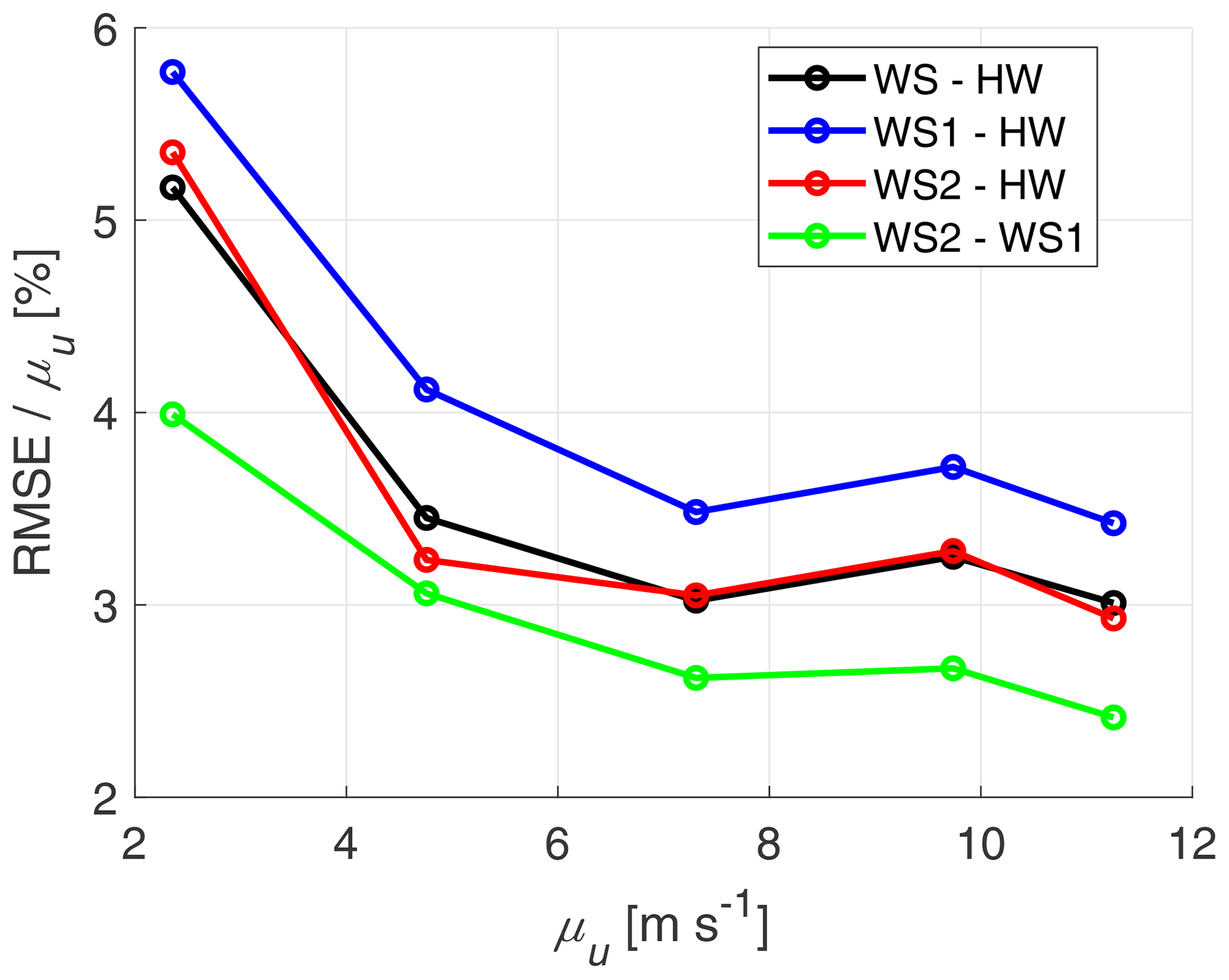
Figure 19 Normalised root-mean-square error of the measured wind speed with respect to the hot-wire anemometer for each of the five cases at 451.7 Hz.

Two different measures for the performance of the WindScanners besides the correlation analysis are the mean average error (MAE) and the root-mean-square error (RMSE) with respect to the hot wire, as illustrated by Figs. 18 and 19, respectively. Both are normalised with respect to the mean hot-wire wind speed μ_u and plotted as a function of the same variable, corresponding to the statistics in Table 4. Please consider that a hot-wire calibration correction factor of 0.948 has been implemented here, as explained before in Sect. 2.4.

When observing the MAE curves excluding the first measurement (Case 2a), there seems to be a relative bias for both WindScanners, around 0.2 % and 0.9 % respectively, which also affects the dual-Doppler reconstruction. There also seems to be a bias of around 0.9 % between WindScanner 1 and 2, for which different properties and tolerances of the optical systems of the respective WindScanners are considered the most likely reason. Whereas the MAE signifies measurement bias, the RMSE gives a better indication of the measurement uncertainty. The RMSE shows a decreasing trend with respect to the mean wind speed and is below 6 % of the mean wind speed for all cases. The lowest RMSE is found between the two WindScanners because of the identical measurement principle. WindScanner 2 performs slightly better than WindScanner 1 in terms of RMSE, whereas the dual-Doppler reconstruction coincides with the former.

Putting the relative errors in perspective of the findings of Pedersen and Courtney (2021), who found a 0.1 % total calibration uncertainty when measuring the speed of a rotating flywheel, it is concluded that additional measurement uncertainties related to the fluctuating wind speed and the atmospheric conditions inside the wind tunnel play an important role.

Figure 20 presents the power spectral density (PSD) function of the time series corresponding to Case 2c. Both WindScanner 2 and the hot wire clearly indicate several peaks for frequencies lower than 1 Hz, which correspond to the periodicity in the gust protocol. As they result from external gust variations, these peaks are not deemed to be due to turbulence and have a much larger scale than the lowest scales detectable by the WindScanners. No differences can be distinguished between the two curves below approximately 3 Hz. Overall the slope of the hot-wire spectrum is close to the $-\mathrm{5}/\mathrm{3}$ Kolmogorov ratio. The spectrum of the WindScanner drops below the hot-wire spectrum earlier than the predicted cut-off frequency, which we have seen before in Figs. 11 and 12. It is worth noticing that the slope of the WindScanner spectrum is not constant but first has a large negative tendency and later bends back upwards to a nearly horizontal curve for frequencies above 200 Hz. This phenomenon will be explained and modelled in Sect. 4.3.

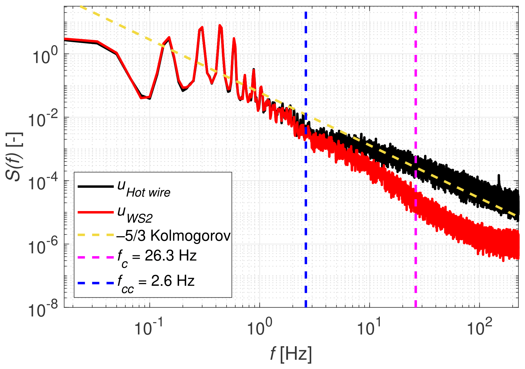
Figure 20 Spectrum of WindScanner 2 and the hot-wire anemometer for a coefficient of variation of 12.9 % (Case 2c).

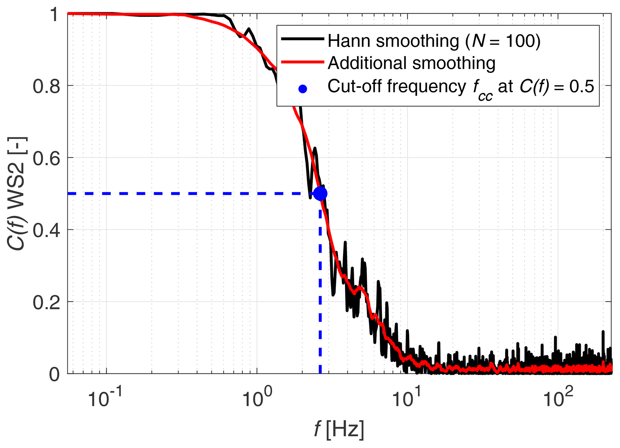
Figure 21 Coherence between WindScanner 2 and the hot-wire anemometer for a coefficient of variation of 12.9 % (Case 2c).

A different method for addressing the differences between the hot-wire and CW-lidar time series in the frequency domain is the magnitude-squared coherence estimate, which relates two time series using the Welch's averaged, modified periodogram method. It is expressed by Eq. (16):

$$\begin{array}{}\text{(16)}& C(f{)}_{\mathrm{WS}\mathrm{2}}={\displaystyle \frac{\left|S\right(f{)}_{\mathrm{WS}\mathrm{2},\mathrm{HW}}{|}^{\mathrm{2}}}{S(f{)}_{\mathrm{WS}\mathrm{2}}\cdot S(f{)}_{\mathrm{HW}}}},\end{array}$$

where S(f)_WS2 and S(f)_HW are the PSD functions of the CW-lidar and hot-wire time series, respectively, and S(f)_WS2,HW is the cross-PSD between the two time series. Figure 21 shows the magnitude-squared coherence for WindScanner 2 for Case 2c, based on the lidar and hot-wire time series, after having been smoothed by using 100 overlapping Hann windows. Below 1 Hz there is an excellent coherence between the hot wire and WindScanner, which means that all coherent structures with scales up to 1 Hz can be measured adequately in agreement by both sensors. Based on this coherence curve, we estimate the coherence-based cut-off frequency of the WindScanner measurement as the frequency at which the coherence drops down to a value of 0.5, indicated with a blue dot in Fig. 21, i.e. f_cc=2.6 Hz for this case. When having a closer look at the frequency spectrum in Fig. 20, it can be seen that this value corresponds quite well to the point at which the WindScanner spectrum begins to deviate from the hot-wire spectrum. This also holds true for the spectra of the other cases.

Table 5 Estimated probe volume and coherence-based cut-off frequencies, f_c and f_cc respectively, of the spectrum of WindScanner 2 with respect to the hot wire.

In Table 5 the cut-off frequencies of all seven cases are summarised. The probe volume cut-off frequency f_c is estimated according to Taylor's frozen turbulence hypothesis, as explained before in Sect. 4.1. There is a characteristic ratio of 7.7 to 10.9 between the two definitions of the cut-off frequency, which means that Taylor's frozen turbulence hypothesis in combination with the probe volume filtering is not sufficient to explain the lidar measurement principle.

4.3 Modelling of WindScanner characteristics in the frequency domain

After having verified the basic statistics, now the model described in Sect. 3.2 is implemented and evaluated. The modelled lidar spectrum is generated by applying the methodology on the measured hot-wire spectrum. Figures 22, 23 and 24 correspond to the spectra for WindScanner 2 shown earlier in Figs. 11, 12 and 20, respectively, but are now extended with two additional curves each: the modelled lidar spectrum for a perfect alignment of β=0^∘ excluding noise, shown in green, only taking into account the Lorentzian filter that resembles the probe length averaging, and the modelled lidar spectrum for the actual case with a misalignment of β=15.1^∘ (see Table 3) including noise, shown in cyan, taking into account the Lorentzian filter as well as a randomly generated white noise term, resembling the full model according to Eq. (10). Please note that the latter curve is not valid for large-scale structures, since it is derived for the inertial sub-range and is therefore only plotted for the region above 1 Hz.

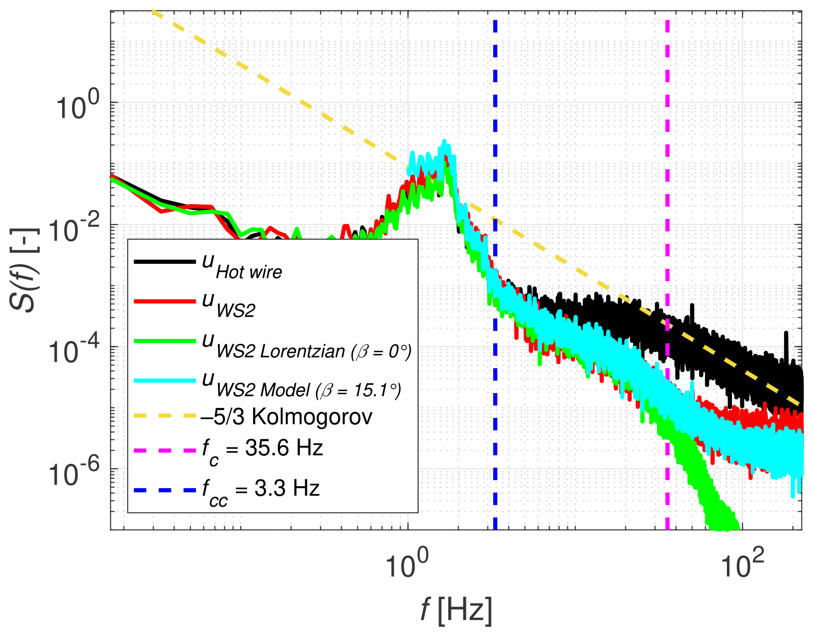
Figure 22 Spectrum of WindScanner 2 (measurements and model) for a turbulence intensity of 3 % (Case 1a).

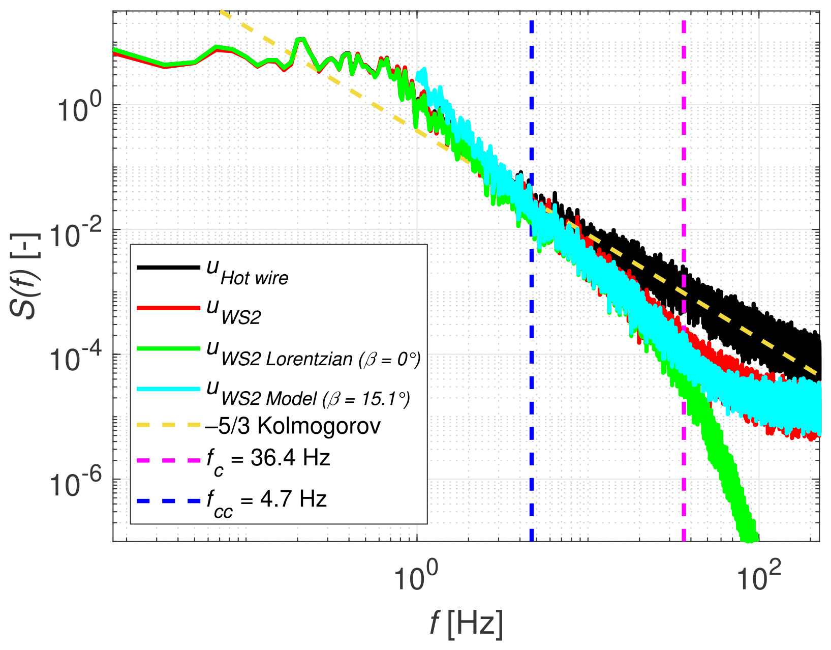
Figure 23 Spectrum of WindScanner 2 (measurements and model) for a turbulence intensity of 22 % (Case 1b).

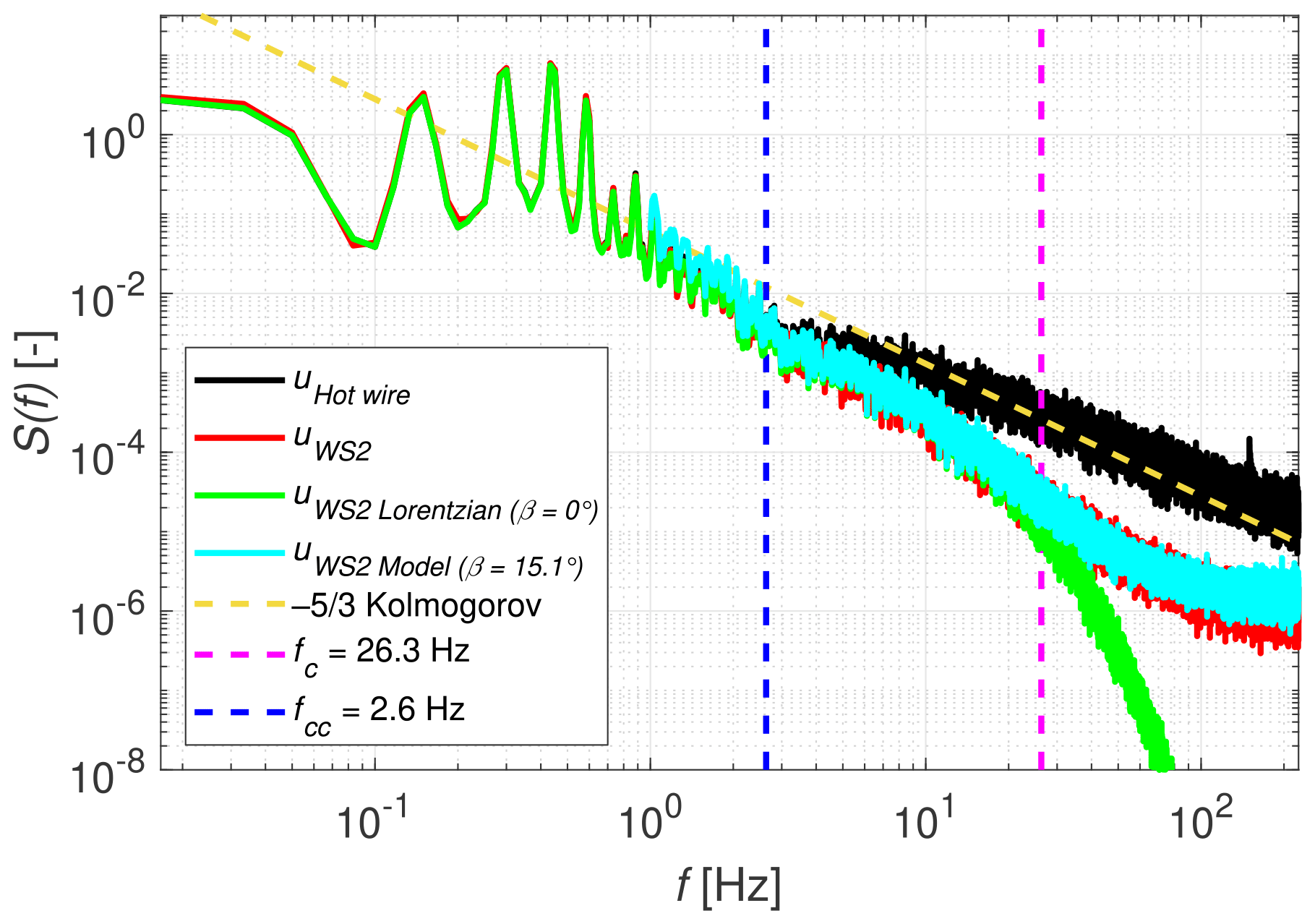
Figure 24 Spectrum of WindScanner 2 (measurements and model) for a coefficient of variation of 12.9 % (Case 2c).

For all three cases it can be seen that the Lorentzian filter model excluding white noise follows the actual WindScanner measurement spectrum, until the probe volume cut-off frequency f_c is reached, after which it drops significantly. This means that the smallest fluctuations, which are within the lidar's probe volume, are filtered out completely. This implies a discrepancy with the measured spectrum for the highest frequencies, where the lidar measurement does not show such a harsh drop-off. When extending the model to its complete form, which includes both the 15.1^∘ misalignment and the noise term ${\mathit{\sigma }}_{\mathit{\eta }}^{\mathrm{2}}{S}_{\mathit{\eta }}\left(f\right)$, we find a spectrum that closely resembles the measured WindScanner 2 spectrum in a qualitative way.

For the definition of the standard deviation of the white noise, the function of the energy dissipation rate and the mean wind speed expressed by Eq. (11) seems to be effective. Although we assumed the noise to be white and thus uncorrelated to the measured wind speed in the time domain, we clearly observed an increase in the manually tuned σ_η with increasing energy in the flow, confirming to us that the level of the noise in a CW-lidar spectrum is partly influenced by global flow parameters. The performance of the model can be addressed by looking at the difference between the Lorentzian filter model excluding noise and the full model including noise in Figs. 22, 23 and 24 for the frequency region f>f_c, which shows a good agreement between the measured and modelled spectrum. However, the model was based on only seven cases in a controlled environment and for a single lidar configuration with a fixed misalignment angle β. To further verify this model, additional research for a wider variety of wind conditions, turbulence intensities and misalignment angles is required. Also, the fitted constant C in Eq. (11) has a unit of metres per second squared (m s⁻²), indicating that there could be additional parameters playing a role, for example, intrinsic time and length scales or lidar parameters.

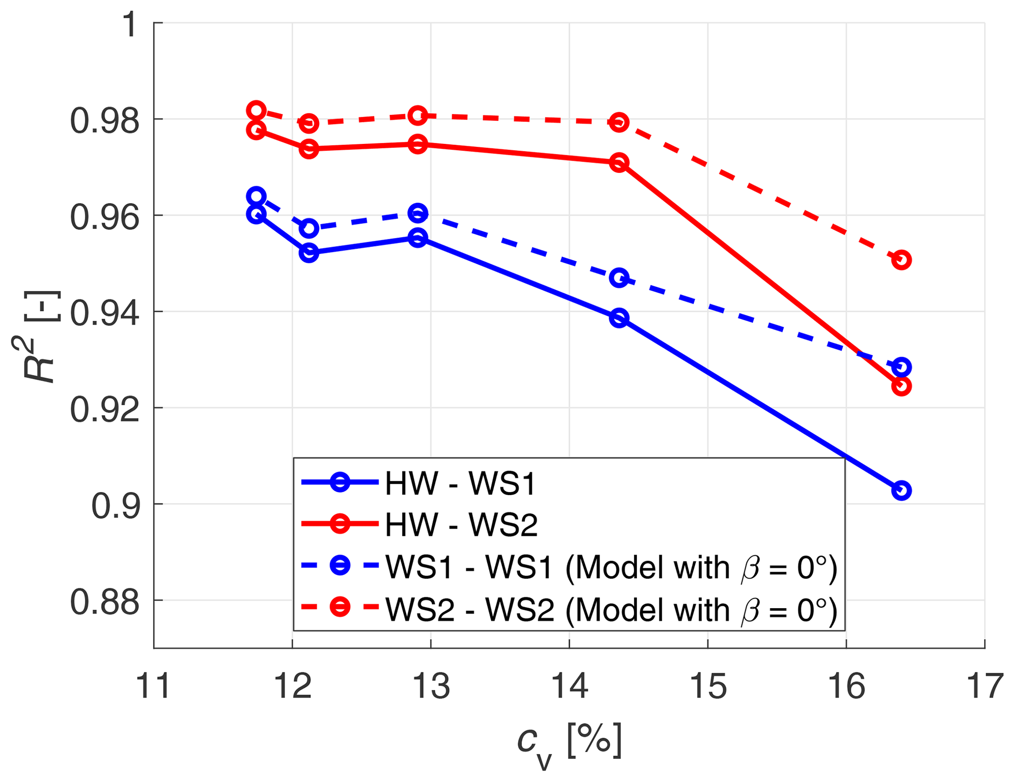
Figure 25 Correlation between WindScanner and hot-wire time series (solid lines) and between modelled and actual WindScanner time series (dashed lines), as a function of the coefficient of variation.

As an additional verification of the approach, we address the correlation between the modelled WindScanner time series with the actual measurement (see Fig. 25). The solid blue and red lines resemble the exact same curves as in Fig. 17 as a reference. The dashed lines correspond to the respective modelled WindScanner time series. Note that these are the results of the time domain implementation of the model (see Eq. 6) and therefore do not consider the misalignment with the flow. However, the white noise term is included. Over the entire range of cases, the modelled lidar measurement correlates better to the actual WindScanner measurement than the non-filtered hot-wire time series does, even including the white noise. This confirms that the model was implemented in a physically realistic way and can successfully resemble the CW lidar.

The potential application of the proposed analytical model is that one could derive the turbulence spectrum directly from the CW-lidar measurement, by rearranging Eq. (10). In this paper a hot wire was used as a reference, but the model only depends on it for the initial tuning of the model through constant C and the calculation of the energy dissipation rate ε. If these parameters are derived through alternative methods, and the model is consolidated by means of additional research for different situations, one could potentially resolve the full power spectral density from the CW-lidar measurement alone. The spectral model was established by analysing the flow inside a controlled environment, but it is hypothesised that it should also be valid for wind speed measurements in the atmospheric boundary layer. However, further research is required to evaluate this.

5 Conclusions

This paper conducted a thorough analysis on the performance of a WindScanner lidar setup for a variety of turbulent wind conditions in a wind tunnel.

It was concluded that the correlation between WindScanner and hot wire was better for a turbulence intensity of 22 % than for a 3 % reference, under similar mean wind speeds. This was mainly influenced by the nature of the turbulence fluctuations, as a result of the active grid protocol used to generate the high-turbulent case. An identical active grid protocol was used to address five different cases, with mean wind speeds varying between 2.36 and 11.25 m s⁻¹ and corresponding coefficients of variation varying between 11.7 % and 16.4%. Here it is found that the correlation improves for higher wind speeds and lower coefficients of variation, which is regarded as a more realistic tendency for atmospheric turbulence.

Analysis of the MAE and RMSE of the WindScanner time series with respect to the hot-wire revealed different biases for each of the two lidars, where WindScanner 2 has a higher MAE but a lower RMSE than WindScanner 1. The dual-Doppler reconstruction tends to coincide with whichever WindScanner has the lower MAE or RMSE values. The MAE and RMSE for Cases 2a–2e are consistently below 1.5 % and 6 % of the mean wind speed, respectively. Please note that the uncertainty on both error estimates might be significant, since a correction factor of 0.948 was applied to the hot-wire measurements after having discovered a faulty hot-wire calibration.

The turbulence spectrum of the WindScanner measurement matches very well with the hot-wire spectrum at the lowest frequencies, corresponding to larger eddy structures of the turbulent flow. However, the WindScanner spectrum starts to deviate from the hot-wire spectrum at frequency which is an order of magnitude lower than the probe volume cut-off frequency. For this reason an alternative way to define the cut-off frequency is proposed, i.e. the frequency at which the coherence drops below 0.5, which corresponds better to the point where a clear deviation of the lidar power spectrum from the hot-wire spectrum takes place. It is hypothesised that the effective probe length exceeds well over the full width at half maximum, but no concrete alternative definition for the probe length is proposed.

A model was established that can be used to simulate a lidar measurement time series or power spectrum based on a probe length filter resembled by a Lorentzian function, acting on the hot-wire time series, and randomly generated white noise. Not only does the resulting model match the actual lidar measurement qualitatively in the frequency domain, but its time domain implementation also correlates better to the actual WindScanner measurement than the non-filtered hot-wire time series does. Modelling of the lidar measurement solely with a Lorentzian probe volume filter was proven insufficient, since the angle β between the line-of-sight pointing direction and the mean flow direction and random measurement noise also defines the shape of the measured spectrum. The proposed model, which does cover these aspects, can potentially be used to resolve the power spectral density function of atmospheric flow on the basis of CW-lidar measurements alone, overcoming the inherent shortcomings of the measurement principle.

It was observed that the noise in the lidar spectrum is, although uncorrelated with the wind speed time series, proportional to both the mean wind speed and the energy dissipation rate in the flow. However, the model of the lidar noise standard deviation has to be further investigated, for example, by performing additional measurements.

Appendix A

For modelling the spectral shape of CW-lidar measurements, we utilised physical methods. According to Kristensen et al. (2011), an analytical approach for the spectral density transfer function of a CW lidar, measuring a flow within isotropic three-dimensional turbulence within the inertial sub-range under a fixed angle, can be expressed as such:

$$\begin{array}{}\text{(A1)}& \begin{array}{rl}f(\mathit{\beta },k,L)& ={\displaystyle \frac{\mathrm{1}}{\mathrm{5}\sqrt{\mathit{\pi }}}}{\displaystyle \frac{\mathrm{\Gamma }(\mathrm{1}/\mathrm{3})}{\mathrm{\Gamma }(\mathrm{5}/\mathrm{6})}}{\sin }^{\mathrm{5}/\mathrm{3}}\left(\mathit{\beta }\right)(kL{)}^{-\mathrm{5}/\mathrm{3}}\\ & +{\displaystyle \frac{\mathrm{9}}{\mathrm{110}}}\left(\mathrm{7}\cos \right(\mathrm{2}\mathit{\beta })-\mathrm{5})e^{-kL}(kL{)}^{-\mathrm{2}/\mathrm{3}},\end{array}\end{array}$$

where β represents the angle between the lidar's line-of-sight direction and the mean flow direction, k is the wave number, L is the probe length of the lidar measurement and Γ is the gamma function.

In the next step, we express the spectral density function for an infinitesimally small probe volume (L→0) and for a perfectly aligned measurement (β=0^∘):

$$\begin{array}{}\text{(A2)}& f(\mathrm{0},k,L){\mid }_{L\to \mathrm{0}}={\displaystyle \frac{\mathrm{9}}{\mathrm{55}}}(kL{)}^{-\mathrm{2}/\mathrm{3}}.\end{array}$$

This expression allows us to define the theoretical spectral transfer function as

$$\begin{array}{}\text{(A3)}& T\left(\mathit{\beta },k,L\right)={\displaystyle \frac{f(\mathit{\beta },k,L)}{f(\mathrm{0},k,L){\mid }_{L\to \mathrm{0}}}}.\end{array}$$

Substituting this for $f(\mathit{\beta },k,L)$ and $f(\mathrm{0},k,L){\mid }_{L\to \mathrm{0}}$ yields

$$\begin{array}{}\text{(A4)}& \begin{array}{rl}T\left(\mathit{\beta },k,L\right)& ={\displaystyle \frac{\mathrm{11}}{\mathrm{9}\sqrt{\mathit{\pi }}}}{\displaystyle \frac{\mathrm{\Gamma }(\mathrm{1}/\mathrm{3})}{\mathrm{\Gamma }(\mathrm{5}/\mathrm{6})}}{\sin }^{\mathrm{5}/\mathrm{3}}\left(\mathit{\beta }\right)(kL{)}^{-\mathrm{1}}\\ & +{\displaystyle \frac{\mathrm{1}}{\mathrm{2}}}\left(\mathrm{7}\cos \right(\mathrm{2}\mathit{\beta })-\mathrm{5})e^{-kL}.\end{array}\end{array}$$

The last step is the expression of the transfer function as a function of frequency, i.e. T(f,β). We make use of the definition of the wave number k:

$$\begin{array}{}\text{(A5)}& k={\displaystyle \frac{\mathrm{2}\mathit{\pi }}{\mathit{\lambda }}}={\displaystyle \frac{\mathrm{2}\mathit{\pi }f}{u_{\mathrm{\infty }}}},\end{array}$$

where λ is the wavelength, and u_∞ is the free-stream flow velocity.

We can now further simplify the formula by taking into account the previously defined cut-off frequency f_c according to Eq. (14):

$$\begin{array}{}\text{(A6)}& f_{\mathrm{c}}={\displaystyle \frac{\mathrm{1}}{\mathrm{2}}}{\displaystyle \frac{u_{\mathrm{\infty }}}{L}}.\end{array}$$

Combining the aforementioned equations, we can define

$$\begin{array}{}\text{(A7)}& kL=\mathit{\pi }{\displaystyle \frac{f}{f_{\mathrm{c}}}},\end{array}$$

which allows us to express the spectral transfer function as

$$\begin{array}{}\text{(A8)}& \begin{array}{rl}T(\mathit{\beta },f)& ={\displaystyle \frac{\mathrm{11}}{\mathrm{9}\sqrt{\mathit{\pi }}}}{\displaystyle \frac{\mathrm{\Gamma }(\mathrm{1}/\mathrm{3})}{\mathrm{\Gamma }(\mathrm{5}/\mathrm{6})}}{\sin }^{\mathrm{5}/\mathrm{3}}\left(\mathit{\beta }\right){\left(\mathit{\pi }{\displaystyle \frac{f}{f_{\mathrm{c}}}}\right)}^{-\mathrm{1}}\\ & +{\displaystyle \frac{\mathrm{1}}{\mathrm{2}}}\left(\mathrm{7}\cos \right(\mathrm{2}\mathit{\beta })-\mathrm{5})e^{-\mathit{\pi }\frac{f}{f_{\mathrm{c}}}}.\end{array}\end{array}$$

For the special case in which β=0^∘, corresponding to the situation where the lidar's line-of-sight direction is aligned with the mean wind direction, the transfer function reduces to the simple form:

$$\begin{array}{}\text{(A9)}& T\left(f\right)=e^{-\mathit{\pi }\frac{f}{f_{\mathrm{c}}}}.\end{array}$$

Appendix B

In order to model the noise standard deviation σ_η, we performed an empirical parameter study. We initially assumed that the noise in a lidar measurement should be related to random fluctuations of the backscattered signal only and that this is a property inherent to the lidar measurement principle and not to the physical properties of the turbulent flow. However, in our analysis we saw a convincing increase of the noise level for more energetic flows with higher wind speeds. We have evaluated various possible dependencies of σ_η on parameters such as the ambient temperature, the mean and standard deviation of the measurement time series, and the energy dissipation rate. In the following, we describe the procedure for the empirical analysis of the lidar spectral noise estimate:

1. For each case (1a, 1b and 2a–2e), we manually tuned the lidar noise standard deviation σ_η to the model in Eq. (10) for the best possible match between modelled and measured lidar spectrum, in particular for the high-frequency range.

2. With a linear regression, we then tried to identify a parameter or a combination of parameters that could best match those tuned values for σ_η.

3. The best fit was found for the square root of the product of energy dissipation rate ε and mean wind speed μ_u. This expression outperformed the dependencies on either of those sole parameters.

Figure B1 displays the convincing linear fit through the seven available cases, indicating the plausibility of Eq. (11).

Figure B1 Plot of the relationship between the lidar spectral noise standard deviation σ_η and the square root of the energy dissipation rate multiplied by the mean wind speed.