the Creative Commons Attribution 4.0 License.
the Creative Commons Attribution 4.0 License.
 | 16 Mar 2022
Improved monitoring of shipping NO2 with TROPOMI: decreasing NOx emissions in European seas during the COVID-19 pandemic
Tobias Christoph Valentin Werner Riess
Klaas Folkert Boersma
Jasper van Vliet
Wouter Peters
Maarten Sneep
Henk Eskes
Jos van Geffen
TROPOMI (TROPOspheric Monitoring Instrument) measurements of tropospheric NO2 columns provide powerful information on emissions of air pollution by ships on open sea. This information is potentially useful for authorities to help determine the (non-)compliance of ships with increasingly stringent NOx emission regulations. We find that the information quality is improved further by recent upgrades in the TROPOMI cloud retrieval and an optimal data selection. We show that the superior spatial resolution of TROPOMI allows for the detection of several lanes of NO2 pollution ranging from the Aegean Sea near Greece to the Skagerrak in Scandinavia, which have not been detected with other satellite instruments before. Additionally, we demonstrate that under conditions of sun glint TROPOMI's vertical sensitivity to NO2 in the marine boundary layer increases by up to 60 %. The benefits of sun glint are most prominent under clear-sky situations when sea surface winds are low but slightly above zero (±2 m s−1). Beyond spatial resolution and sun glint, we examine for the first time the impact of the recently improved cloud algorithm on the TROPOMI NO2 retrieval quality, both over sea and over land. We find that the new FRESCO+ (Fast Retrieval Scheme for Clouds from the Oxygen A band) wide algorithm leads to 50 hPa lower cloud pressures, correcting a known high bias, and produces 1–4×10¹⁵ molec. cm−2 higher retrieved NO2 columns, thereby at least partially correcting for the previously reported low bias in the TROPOMI NO2 product. By training an artificial neural network on the four available periods with standard and FRESCO+ wide test retrievals, we develop a historic, consistent TROPOMI NO2 data set spanning the years 2019 and 2020. This improved data set shows stronger (35 %–75 %) and sharper (10 %–35 %) shipping NO2 signals compared to co-sampled measurements from OMI. We apply our improved data set to investigate the impact of the COVID-19 pandemic on ship NO2 pollution over European seas and find indications that NOx emissions from ships reduced by 10 %–20 % during the beginning of the COVID-19 pandemic in 2020. The reductions in ship NO2 pollution start in March–April 2020, in line with changes in shipping activity inferred from automatic identification system (AIS) data on ship location, speed, and engine.
- Article
(7705 KB) - Full-text XML
-
Supplement
(362 KB) - BibTeX
- EndNote


Emissions of nitrogen oxides (NOx = NO + NO2) have several primary and secondary effects on air quality, human health, and the environment. NOx is a toxic gas itself (WHO, 2003) and contributes to the formation of secondary pollutants and ozone. Ozone close to the Earth's surface is a toxic pollutant which can lead to respiratory problems and has negative effects on plant growth and crop yield (e.g., Wang and Mauzerall, 2004). NOx also contributes to acid deposition and eutrophication, harming sensitive ecosystems (European Environment Agency, 2019).
The international shipping sector is a strong source of NOx and other air pollutants to the atmosphere (e.g., Eyring et al., 2010). Previous studies suggest that international shipping makes up annual emissions of 2.0–10.4 TgN (Crippa et al., 2018; Eyring et al., 2010; Johansson et al., 2017) or 15 %–35 % of total anthropogenic NOx emissions worldwide. While cars, the power sector, and industry have shown substantial reductions in their emissions over the last 10–20 years in Europe and the United States (Curier et al., 2014; Hassler et al., 2016), NOx emissions from shipping activity have increased (De Ruyter de Wildt et al., 2012; Boersma et al., 2015), and the number of ship movements and ship size are expected to keep increasing in the future (Eyring et al., 2005; UNCTAD, 2019). Shipping-related air pollution emissions are estimated to lead to 60 000 premature deaths annually, especially in coastal regions (Corbett et al., 2007; Marais et al., 2015).
To mitigate these and other harmful impacts, more stringent regulations on NOx emissions for ships have been implemented in coastal regions and on the open ocean (IMO, 2013). For example, ships built in 2011 or later have to follow Tier II nitrogen emission regulation as defined in MARPOL Annex VI. In so-called Emission Control Areas (ECAs) even more stringent rules apply. From 1 January 2021 onwards, the new MARPOL Annex VI regulation 13 determines that newly built ship engines should be compliant with Tier III in the new ECA in the Baltic and North Sea, which should result in 75 % lower NOx emissions from new ships. The exact limits depend on ship engine speed (IMO, 2013); see Sect. S1 in the Supplement.
For new regulations to be effective, monitoring and verification of ship emissions are required. Traditional compliance monitoring includes national authorities conducting onboard checks of engine certificates and keel-laying date. This is not a direct verification of emissions and can only be done for a limited number of vessels. Other methods are onboard measurements at the ship's exhaust pipe (e.g., Agrawal et al., 2008) or downwind measurements of emission plumes using sniffer techniques or DOAS (differential optical absorption spectroscopy) measurements (e.g., Lack et al., 2009; Berg et al., 2012; McLaren et al., 2012; Pirjola et al., 2014; Seyler et al., 2019). Modern techniques also include airborne platforms such as helicopters, small aircraft (Mellqvist and Conde, 2021; Chen et al., 2005a), or drones (Van Roy and Scheldeman, 2016). While these methods do not require inspectors to board the vessel, they require proximity to the ships monitored and are thus less fit-for-purpose when a large number of ships is to be checked or on open sea away from land. For the above reasons monitoring by satellite remote sensing offers a promising alternative.
Satellite instruments have observed enhancements of NO2 column densities over major shipping routes, e.g., from GOME (Beirle et al., 2004), SCIAMACHY (Richter et al., 2004), and OMI (Vinken et al., 2014b; Marmer et al., 2009). These satellite measurements have recently been continued with new observations from the TROPOMI (TROPOspheric Monitoring Instrument) sensor. With a pixel size of 3.5 km ×5.5 km TROPOMI provides a spatially more resolved evaluation of NO2 pollution patterns compared to its predecessors GOME (40 km ×320 km), SCIAMACHY (30 km×60 km), and OMI (13 km ×24 km). Indeed, previous studies demonstrated TROPOMI's capability to pinpoint emissions from the mining industry (Griffin et al., 2019), emissions patterns within cities (Beirle et al., 2019; Lorente et al., 2019), emissions along a gas pipeline in Siberia (van der A et al., 2020), and even from individual ships in the Mediterranean Sea (Georgoulias et al., 2020). Ding et al. (2020) used TROPOMI NO2 columns and inverse modeling to show NOx emission reductions during the COVID-19 lockdown over urban centers and regions with strong maritime transport.
While the aforementioned studies demonstrate the large potential of TROPOMI and its high resolution, retrieval problems remain. Validation studies (e.g., Griffin et al., 2019; Verhoelst et al., 2021) suggest a 15 %–40 % low bias in TROPOMI tropospheric vertical NO2 (Nv,trop) columns relative to independent in situ and MAX-DOAS (multi-axis differential optical absorption spectroscopy) measurements. Cloud properties present one of the leading sources of uncertainty in trace gas retrieval from space (Boersma et al., 2004; Lorente et al., 2017), and cloud heights used until (and including) v1.3 of the operational TROPOMI retrieval algorithm have been suggested to be biased low (Compernolle et al., 2021). To address this bias in cloud heights, the Royal Dutch Meteorological Institute (KNMI) recently updated the FRESCO+ (Fast Retrieval Scheme for Clouds from the Oxygen A band) cloud retrieval by widening the spectral window, which is supposed to improve the sensitivity to low clouds.
The here-presented study presents and assesses the impact of steps towards an improved monitoring of shipping NO2 with TROPOMI. First, we demonstrate TROPOMI's capability to detect ship emissions applying a typical data selection and compare it to OMI's. We examine previous suggestions of improved retrieval sensitivity over sun glint scenes (Georgoulias et al., 2020). Additionally, we evaluate the new FRESCO+ wide cloud pressure retrieval and its impact on the TROPOMI NO2 columns in v1.4–2.1 of the operational TROPOMI NO2 algorithm. Based on our findings, we create a data set of historical TROPOMI NO2 columns consistent with the v1.4 data allowing for otherwise challenging trend analysis. We conclude with an application of our findings to quantify the effects of the COVID-19 pandemic on ship pollution, a unique opportunity to assess the relationship between the anticipated emission reductions and observed NO2 columns.
2.1 TROPOMI and OMI NO2 column measurements
The European TROPOMI (Veefkind et al., 2012) is on board the Sentinel-5 Precursor launched in October 2017. TROPOMI has a push-broom design with a 2-D detector, which measures back-scattered radiation from the Earth’s atmosphere for viewing zenith angles up to 57∘, in the spectral region from UV to shortwave infrared. The instrument is equipped with a polarization scrambler, simplifying the radiative transfer analysis. The width of the TROPOMI swath is about 2600 km, which results in daily (near-)global coverage with about 25 million measurement points. In band 4, where NO2 is retrieved, TROPOMI provides 450 measurements across-track, with a minimal width of 3.5 km.
The design of OMI is similar to that of TROPOMI, but OMI measures in a smaller spectral range (270–500 nm) (Levelt et al., 2006, 2018). Another important difference is that OMI has only 60 across-track measurements, with the smallest pixels having a width of 25 km. Along track, the resolution of TROPOMI is 7 km (5.5 km since August 2019), compared to 13 km for OMI. Combined, the area of the smallest TROPOMI pixel is 19 km2, while it is 325 km2 for OMI, a factor of 17 improvement in spatial resolution. Both instruments are in a sun-synchronous ascending orbit and have an Equator overpass time of about 13:30 local time.
To retrieve tropospheric NO2 columns, TROPOMI uses a three-step retrieval approach based on the DOAS (differential optical absorption spectroscopy; Platt and Stutz, 2008) technique: first the slant column density (Ns) is retrieved by spectral fitting of a modeled reflectance spectrum to the observed reflectances in the 405–465 nm window (van Geffen et al., 2021b, 2020; Zara et al., 2018). In the second step, data assimilation in the global chemistry transport model 5 (TM5-MP) results in vertical NO2 profiles that are then used to separate the stratospheric and tropospheric contribution to the slant columns (van Geffen et al., 2020; Dirksen et al., 2011). In the last step, air mass factors (AMFs) are calculated (Lorente et al., 2017) to translate the Ns into vertical column densities (Nv). The AMF is calculated using the DAK radiative transfer model (de Haan et al., 1987; Stammes, 2001) and accounts for the viewing and solar geometry, as well as surface properties and cloud effects. Cloud height information is retrieved with TROPOMI's FRESCO+ cloud algorithm (driven by the 761 and 765 nm O2 absorption depths) and cloud fraction from the reflectance levels within the 405–465 nm NO2 fitting window. Other input parameters to the TROPOMI AMF calculation are the surface albedo climatology (Kleipool et al., 2008; 0.5∘ × 0.5∘), a priori NO2 profiles simulated with TM5-MP (Williams et al., 2017; 1∘ × 1∘), and terrain height from Global 3 km Digital Elevation Model (DEM_3KM).
The retrieval of tropospheric NO2 columns (Nv,trop) from OMI (Boersma et al., 2018) proceeds along the same lines and is therefore similar in many aspects. On the other hand, especially spatial resolution, signal-to-noise, and the retrieval of cloud properties differ as highlighted in Table 1.
Clouds have several relevant effects on NO2 retrieval. Clouds shield the lower part of the atmosphere which is most influenced by anthropogenic emissions including those from shipping. Therefore, data users are typically advised to consider scenes with cloud radiance fractions below 50 % (Eskes et al., 2019). Initial validation of TROPOMI NO2 v1.2–1.3 pointed out that the FRESCO+ algorithm retrieves cloud heights close to the surface heights, leading to overestimations in the TROPOMI NO2 AMFs and, consequently, underestimations of the tropospheric NO2 columns (Verhoelst et al., 2021). Accurate knowledge of cloud fraction and height is key for high-quality trace gas column retrievals (e.g., Boersma et al., 2004; van Geffen et al., 2021a). A detailed description of the TROPOMI and OMI cloud algorithms and recent updates therein is given in the following subsection.
Table 1Retrieval settings for the TROPOMI and OMI NO2 retrievals used in this work.
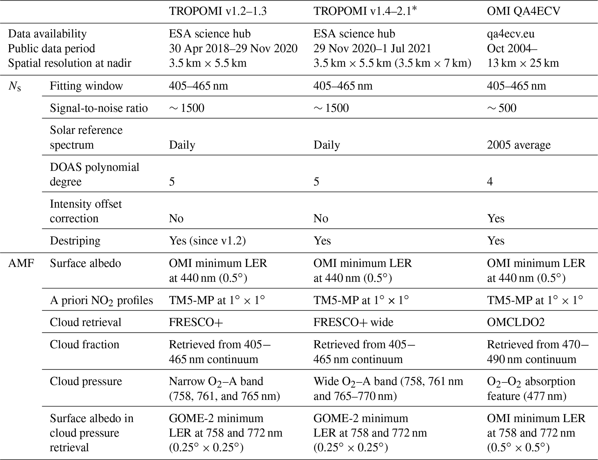
* In addition to improved cloud parameters, TROPOMI v2.1 data has improved further through a better calibration of level-1 spectra, especially in the treatment of outliers and saturation (Ludewig et al., 2020), and through improvements in the NO2 algorithm itself (van Geffen et al., 2021a). Version v2.1 is only used for production of the DDS-2B test data and not for publicly released data. Version v2.2, available publicly as of July 2021, is essentially the same as v2.1.
2.2 Improved TROPOMI FRESCO+, OMI, and VIIRS cloud retrievals
FRESCO+ (Fast Retrieval Scheme for Clouds from the Oxygen A band) retrieves cloud pressures from the relative depth of O2–A band measurements (Koelemeijer et al., 2001; Wang et al., 2008) using three spectral windows at 758–759 nm (continuum, no absorption), 760–761 nm (strong absorption), and 765–766 nm (moderate absorption). In the algorithm, clouds are assumed to be Lambertian reflectors with a fixed albedo of 0.8, consistent with assumptions for the NO2 AMF calculation. The surface albedo assumed in the cloud pressure retrieval is from the GOME-2 minimum Lambertian-equivalent reflectivity (LER) climatology at 758 and 772 nm (Tilstra et al., 2017), which is a potential source of uncertainty in the cloud pressure retrieval as the resolution and overpass time of GOME-2 are different from TROPOMI. FRESCO+ has been compared to other cloud data sets by Compernolle et al. (2021), who reported on tendencies in FRESCO+ to overestimate cloud pressures.
To address the high-bias in TROPOMI FRESCO+ cloud pressures, a new version of the FRESCO+ algorithm was introduced and implemented in the operational NO2 retrieval with the introduction of TROPOMI v1.4 in December 2020. This version, called FRESCO+ wide, uses a wider spectral window for the cloud retrieval (765–770 nm, see Table 1), which includes the flank of the absorption band, where oxygen absorption is weaker than in the center of the O2–A band (761 and 765 nm). Adding weaker O2 absorption features improves the sensitivity to clouds low in the atmosphere. This is not possible from the strong O2 absorption at 761 nm, which is so close to saturation that it becomes difficult to use its absorption depth in order to distinguish between bright reflecting layers at the Earth's surface and reflecting surfaces in the lower atmosphere.
Prior to the implementation of FRESCO+ wide in the operational TROPOMI NO2 retrieval in December 2020, KNMI produced four periods with TROPOMI NO2 test data based on FRESCO+ wide, the so-called diagnostic data set 2B (DDS-2B). DDS-2B contains data from four v1.2–v1.3 periods during 2018–2019 additionally processed with v2.1 of the TROPOMI algorithm. The most significant difference between the two is that v2.1 (and v1.4) uses cloud fractions and AMFs determined from the FRESCO+ wide cloud pressure instead of the FRESCO+ cloud pressures used in v1.2–v1.3 data.
Additionally, we use co-sampled cloud information from the Ozone Monitoring Instrument (OMI) on board of EOS-Aura. The OMI OMCLDO2 retrieval uses the relative depth of the O2–O2 absorption feature at 477 nm to retrieve cloud pressures (Acarreta et al., 2004; Veefkind et al., 2016). The general approach of using Lambertian reflectors is similar to the FRESCO+ algorithm, but an important difference is that the OMCLDO2-algorithm needs to account for Raman scattering and O3 absorption and that the absorption strength of the O2–O2 features is proportional to the square of the O2 concentration, making it more sensitive to low clouds compared to FRESCO+.
We also use cloud information from VIIRS (Visible Infrared Imager Radiometer Suite) on board of the SUOMI National Polar-orbiting Partnership (SNPP) as a completely independent means of verification. SNPP orbits the Earth in a sun-synchronous, ascending node with full daily global coverage and observes the same scenes as TROPOMI within 3 min. We use NASA's CLDPROP L2 VIIRS-SNPP cloud product (Platnick et al., 2017) with a resolution of 750 m at nadir, which provides a cloud mask, cloud (top) pressure, cloud optical thickness (COT), and cloud water phase for each pixel retrieved. The VIIRS retrieval derives a cloud top temperature using an optimal estimation approach in the thermal infrared spectral bands M14–M16 (8.5–12.3 µm). In a subsequent step, these cloud top temperatures are converted to cloud pressures using numerical weather prediction temperature profiles (Heidinger and Li, 2017). In addition to the cloud top pressure, we use the VIIRS cloud optical thickness (COT) to generate (effective) cloud fractions that can be compared directly to the TROPOMI cloud fractions. First, we derive a geometrical cloud fraction by calculating the share of cloudy VIIRS pixels per grid cell. Then, we translate this geometrical cloud fraction fc,geo into a effective cloud fraction fc,eff using
with ac being the cloud albedo. The cloud albedo is calculated from the VIIRS COT and a previously established empirical relationship between cloud optical thickness and cloud albedo for liquid water clouds (Buriez, 2005; Boersma et al., 2016)1.
To evaluate the improvements in the FRESCO+ wide retrieval, we compare daily gridded, co-sampled cloud data from (partly) cloudy pixels seen by TROPOMI (FRESCO+ and FRESCO+ wide), OMI, and VIIRS over parts of the Mediterranean Sea (37.0–41.25∘ N, 2.0–8.0∘ W), the Bay of Biscay (43.5–47.5∘ N, 10.0–3.0∘ E), and Northwest Europe (50.0–53.0∘ N, 4.0–9.0∘ W). These regions represent different surface types (land and ocean), climatological conditions, and pollution levels. We define partly cloudy pixels as all pixels with an effective cloud fraction fc≥0.05. For TROPOMI we additionally apply sufficient quality of retrieval (fQA≥0.5) and a pressure difference between surface pressure and cloud pressure of at least 7 hPa. The last filter is applied to filter out “ghost” clouds coming from sun glint viewing geometries (see Sect. 2.3 below). For OMI, we use the OMCLDO2 cloud properties and take only pixels with solar and viewing zenith angles smaller than 80∘ into account. As Eq. (1) is valid for liquid water clouds only, we select liquid water clouds and reject ice clouds, as indicated by the VIIRS cloud water phase. Around 25 %–30 % of VIIRS pixels are missed due to this filter.
2.3 Sun glint in the TROPOMI NO2 retrieval
The term sun glint refers to particular satellite viewing geometries, under which the ocean acts as a mirror by reflecting sun light directly to the satellite instrument. In the TROPOMI data product pixels that are potentially in sun glint mode are identified based on the combination of their solar and viewing zenith and azimuth angles. The sun glint condition is fulfilled when the scattering angle Θ is smaller than a threshold angle Θmax:
with θ and θ0 being the solar and viewing zenith angles and ϕ and ϕ0 the solar and viewing azimuth angles, respectively (see Fig. S1). For the TROPOMI data products the maximum threshold angle has been set at 30∘. Smaller angles are used before, e.g., for SCIAMACHY and GOME-2 (Loots et al., 2017). The TROPOMI algorithm treats the enhanced albedo as a partially cloudy scene with the cloud pressure located at or close to the sea surface.
2.4 Relationship between NOx emissions and columns
When studying NO2 columns to investigate emission trends, the non-linearity of NOx chemistry needs to be taken into account. For example, the lifetime of NOx depends on the background O3 level, the available sun light, and NOx concentrations themselves (Jacob, 1999). We use a (modeled) β factor to express the sensitivity of relative NO2 column changes to changes in the relative emission strength following the approach in Vinken et al. (2014a) with
where represents the imposed relative change in NOx emission flux and the relative change in subsequently simulated tropospheric NO2 columns. Here we use β values from Vinken et al. (2014b) modeled with GEOS-Chem at 0.5∘ × 0.67∘ and accounting for plume-in-grid chemistry. These β values have a similar spatial resolution as the spatially averaged TROPOMI NO2 signals from ships (see Fig. 9). As we are interested in European seas only, we average β in the area 35–40∘ N and 5∘ E–10∘ W for Gibraltar and 30–37∘ N and 15–35∘ W for the Eastern Mediterranean. We use the resulting β value to estimate relative changes in NOx emissions as
where is the observed relative change in NO2 columns.
2.5 AIS data and ship-specific data
To relate the TROPOMI NO2 columns to shipping activity, we use data from the automatic identification system (AIS) for shipping. Since 2005, the International Maritime Organization (IMO) requires all ships with a gross tonnage over 300 and all passenger ships to carry an AIS transponder. These transponders broadcast static (e.g., identity, size) and dynamic (e.g., position, speed, course) information of the ship, which can be received by other ships, shore stations, and satellites (International Maritime Organization (IMO), 2014). Here we use historical AIS data available to the Dutch Human Environment and Transport Inspectorate (ILT) to assess changes in shipping activity over densely traveled European shipping lanes in 2019 and 2020. We use AIS data of ships in a part of the shipping lane in the Eastern Mediterranean (31.91–34.53∘ N and 25.91–27.67∘ E) and close to the Strait of Gibraltar (35.0–37.0∘ N and 4.0–2.5∘ W). Furthermore, we use information on ship dimensions from the official ship registrations (https://gisis.imo.org/Public/Default.aspx, last access: 20 December 2021) to calculate a ship emission proxy E from ship length L and ship speed v as , as used, for example, in Georgoulias et al. (2020). For the areas and times under study, ship-specific data were available only for 50 % (Gibraltar) and 70 % (Eastern Mediterranean) of the ships.
We start with demonstrating TROPOMI's capabilities to detect shipping NO2 by applying established data selection criteria. Next, we show steps to optimize monitoring of ship emissions by making use of sun glint (Sect. 3.2) and recent improvements in the cloud retrieval (Sect. 3.3) and compare the improved TROPOMI data to OMI data in Sect. 3.4. We end with an application of our findings to quantify NO2 emission reductions from shipping due to COVID in 2020 in Sect. 3.5.
3.1 Detection of NO2 pollution over European shipping lanes
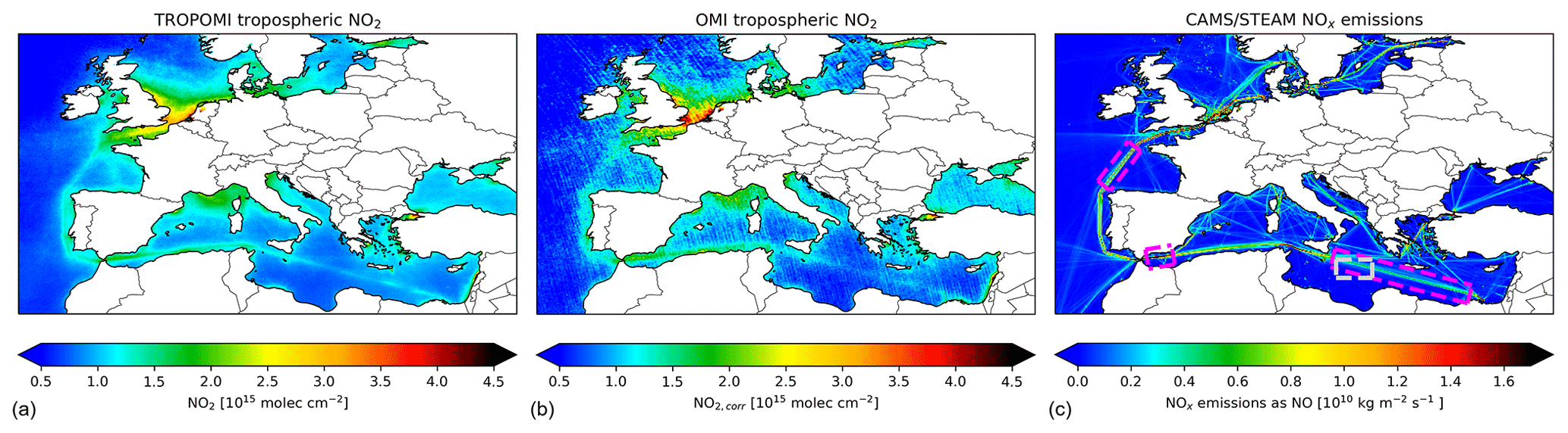
Figure 1Summertime (May–September) mean tropospheric NO2 columns from TROPOMI (a) and OMI (b) over European seas in 2019. Panel (c) shows the summertime mean NOx emissions from the CAMS/STEAM emission inventory (Granier et al., 2019; Johansson et al., 2017). The gray and pink rectangles in the center panel indicate areas used in Sect. 3.2 and 3.4, respectively.
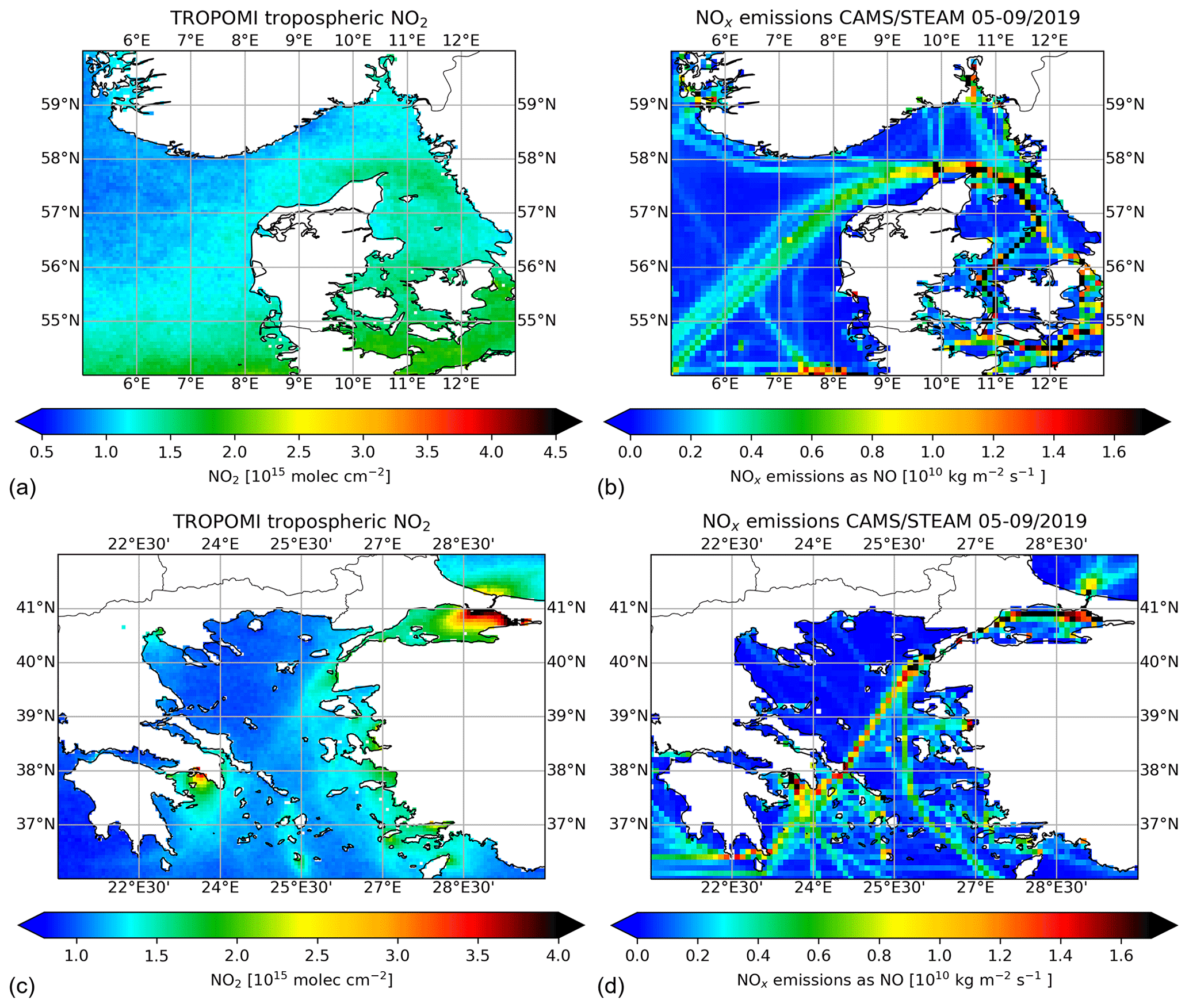
Figure 2The 2019 summertime mean (May–September) tropospheric NO2 columns from TROPOMI (a, c) and summertime mean NOx emissions from the CAMS/STEAM emission inventory (b, d; Granier et al., 2019; Johansson et al., 2017) of shipping lanes around Denmark (a, b) and the eastern Aegean Sea (c, d) for the first time detected with satellites.
TROPOMI detects unprecedented spatial detail in shipping NO2 over busy shipping routes. Figure 1 shows the summertime mean (May–September 2019) NO2 columns from TROPOMI and OMI averaged to a common 0.0625∘ × 0.0625∘ grid, as well as CAMS/STEAM NO2 emissions (Granier et al., 2019; Johansson et al., 2017) for the same period. We find a clear signal of shipping NO2 in the TROPOMI data west of Portugal and from the Strait of Gibraltar to the east. There are further indications of enhanced NO2 related to shipping in the Bay of Biscay from the tip of Brittany towards the northwest of Spain, and in the Eastern Mediterranean from the south of Sicily towards the Suez Canal. Previous studies reported NO2 enhancements over these shipping lanes with other satellites (e.g., by OMI; Vinken et al., 2014b). Additionally, we see a clear NO2 enhancement in the Aegean Sea between Istanbul and the Greek islands, as well as around Denmark, as shown in Fig. 2, which to our knowledge have not been observed by satellite instruments previously. Furthermore, (clear) hints of shipping activity can be seen in the Baltic Sea, the eastern Aegean Sea, the Adrian Sea, northeast of Corsica, the British Channel, and several forks in the Eastern Mediterranean and southeast of Sicily, which are all present as shipping lanes in CAMS/STEAM emissions. Corresponding zoomed-in maps of TROPOMI tropospheric NO2 and CAMS/STEAM emissions are shown in Appendix A. For the analysis, we selected mostly clear-sky pixels with a quality assurance value (fQA) of 0.75 or higher as recommended in the TROPOMI (Eskes et al., 2019) and (equivalent settings) OMI user manuals (Boersma et al., 2017). These enhancements are not an artifact in the retrieval coming from the AMF calculation (see Sect. 2.1) as they are visible in tropospheric vertical column densities Ntrop,geo using a geometric AMF (see Appendix B) shown in Fig. B1.
TROPOMI and OMI show a comparable high spatial correlation to CAMS/STEAM emission data of R=0.93 and R=0.91, respectively. For the calculation, we brought OMI and TROPOMI tropospheric data to the CAMS resolution (0.1∘ × 0.1∘) and selected only grid cells over the Mediterranean Sea. This was done to ensure comparable meteorological and chemical conditions. Next, we binned the data by emission strength in bins of kg m−2 s−1. A reduced major axis regression of all bins with more than 10 entries leads to the correlation coefficients given above. Corresponding scatter plots can be found in Fig. C1. The y-axis intercept of 1.07 (1.05) ×1015 molec. cm−2 for TROPOMI (OMI) represents the mean background NO2 column over the summertime Mediterranean. Other emission bin sizes lead to slightly different but comparable regression results.
Besides the higher resolution of the TROPOMI instrument, TROPOMI Nv,trop thus has a comparable spatial correlation with emission inventories when compared to OMI's. The distinct shipping lanes visible in Figs. 1 and B1 visualize TROPOMI's unprecedented capabilities to detect shipping NO2.
3.2 Sun glint
For situations of sun glint (see Sect. 2.3) the usually dark ocean appears bright in the TROPOMI data, leading to a strong increase in the effective scene albedo with decreasing scattering angle as shown in Fig. 3a. Figure 3b shows that the increase in scene albedo leads to substantially higher vertical sensitivities, as diagnosed by the averaging kernels (AKs) in the operational TROPOMI NO2 product. The sensitivity increased most in the lowest vertical layer, where the kernel values are on average ≈60 % higher for sun glint compared to non-sun glint circumstances (0.44 vs. 0.28). Increased albedo generally enhances a satellite sensor's sensitivity to NO2 concentrations in the lower atmosphere (e.g., Eskes and Boersma, 2003), and sun glint scenes have been tentatively used previously to attribute shipping plumes to individual ships in the Mediterranean Sea (Georgoulias et al., 2020).
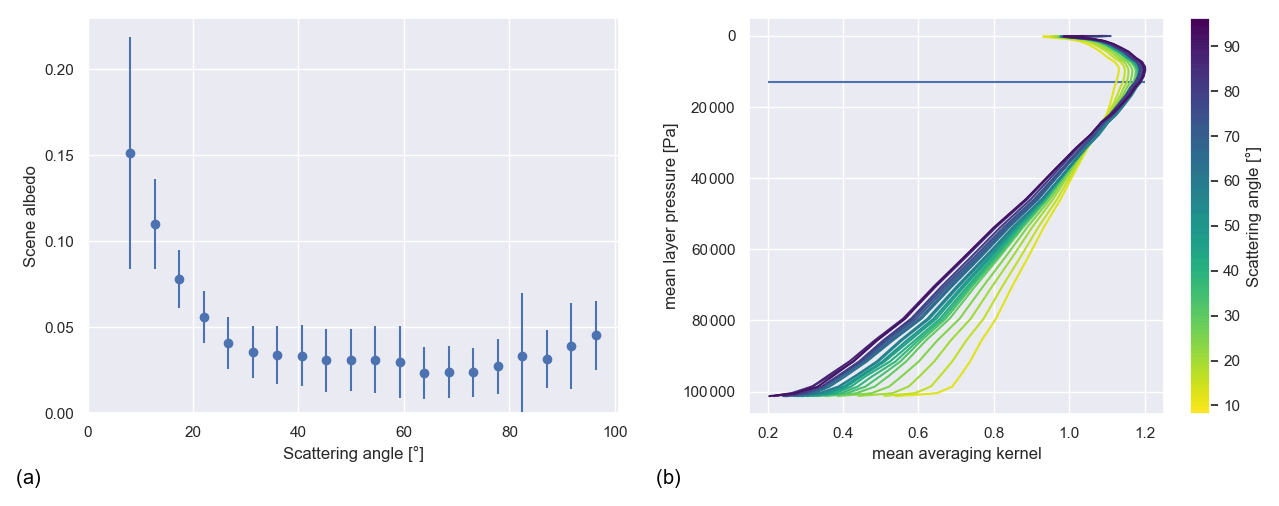
Figure 3(a) Change in effective scene albedo with scattering angle over the Central Mediterranean north of Libya in June–July–August 2018 (see gray rectangle in Fig. 1c, ≈200 000 data points in total). The error bars indicate the standard deviation of each bin. (b) Mean averaging kernel (profiles) for different scattering angles, sampled as for (a). Only pixels with cloud radiance fractions < 0.25 or Pa were selected. The blue line in (b) indicates the average tropopause altitude.
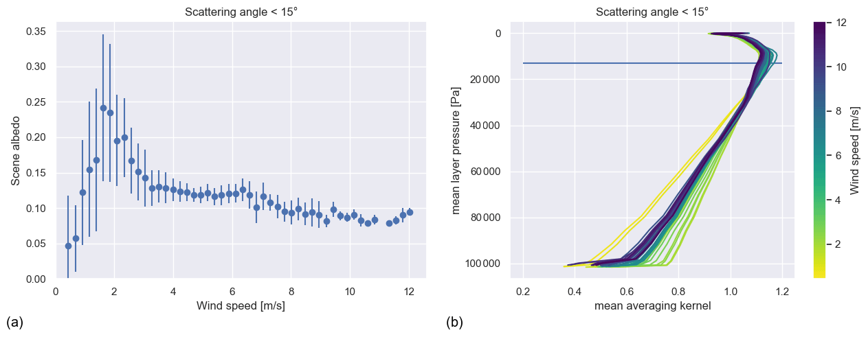
Figure 4(a) Change in effective scene albedo with wind speed over the Central Mediterranean north of Libya in June–July–August 2018 (see gray rectangle in Fig. 1c) for scenes with scattering angles smaller than 15∘ (≈22 000 data points in total). The error bars indicate the standard deviation of each bin. (b) Mean averaging kernel (profiles) for different wind speeds, sampled as for (a). Only pixels with cloud radiance fractions <0.25 or Pa were selected. The horizontal blue line in (b) indicates the average tropopause altitude.
The scene albedo and vertical sensitivity can be further increased by focusing on scenes with low–moderate wind speeds (≈2 m s−1) as wind-induced waves are expected to change the reflectivity. Fig. 4a shows the relationship between effective scene albedo and wind speed for scenes with small scattering angles Θ≤15∘. For very low wind speeds the mean scene albedo is almost as small as for non-sun glint scenes and smaller than for all other wind speeds. For wind speeds between 1.5 and 2.0 m s−1 we find an effective scene albedo of almost 0.25, which is approximately double compared to the average for these scattering angles and more than 5 times as high as for non-sun glint scenes. For higher wind speeds the scene albedo decreases to around 0.10. In Fig. 4b the effect on the averaging kernel profile is shown. As expected low wind speeds lead to the smallest AK in the lower atmosphere, whereas wind speeds between 1.5 and 2.0 m s−1 show the largest AKs close to the sea surface. This relationship can be understood in terms of wind-induced sea surface roughness (Cox and Munk, 1956). Both very low and strong winds limit the probability that a scattering angle Θ≤Θmax leads to sun glint effects at the sensor: For very low wind speeds, the sea surface is effectively flat, leading to sun glint only for very small scattering angles Θ≪Θmax, whereas for strong winds the sea surface is so rough that the sun light is reflected in all directions, making the reflections towards the satellite instrument unlikely.
Additionally, we find that sun glint scenes can be used with confidence for detecting ship pollution signals from UV–Vis spectrometers such as TROPOMI, and the usage of sun glint data should be encouraged. The (normalized) tropospheric slant columns (, see Appendix B) observed under sun glint conditions are 20 %–25 % higher than under non-sun glint conditions as shown in Fig. 5a. Vertical profiles of NO2 over oceans typically feature enhancements from ships within the marine boundary layer and small background levels above (e.g., Chen et al., 2005b; Boersma et al., 2008; see Fig. 1). Therefore, it is no surprise that the AK increases in the lower atmosphere lead to small but detectable increases in (tropospheric) slant columns over the study region covering a frequently traveled shipping lane.
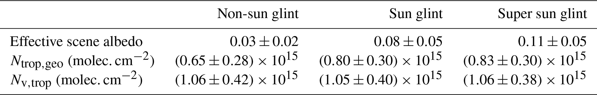
The enhanced slant columns are correctly accounted for by increased AKs leading to reliable retrievals under sun glint. Figure 5b compares the tropospheric vertical columns reported in the official TROPOMI NO2 product sampled under sun glint compared to non-sun glint conditions. The differences between the distributions are only small. Mean values for scene albedo, (normalized) tropospheric slant columns, and tropospheric vertical columns reported in the official TROPOMI NO2 product for different scattering angles are summarized in Table 2.
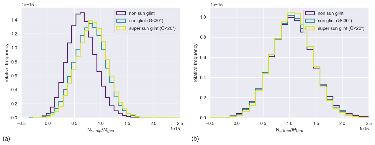
Figure 5(a) Probability distribution of tropospheric NO2 columns () over the Central Mediterranean north of Libya in June–July–August 2018 (see grey rectangle in Fig. 1c) taken under non-sun glint, sun glint (Θ≤30∘), and super sun glint (Θ≤20∘). (b) Probability distribution of tropospheric NO2 columns in the official TROPOMI NO2 product () for the same data selection.
Table 2Summary of mean effective scene albedo, normalized tropospheric slant column, and Nv,trop for non-sun glint, sun glint (Θ≤30∘), and super sun glint (Θ≤20∘) over the Central Mediterranean north of Libya in June–July–August 2018 (see gray rectangle in Fig. 1c).
3.3 Cloud properties
Here we evaluate TROPOMI’s capability to retrieve realistic cloud parameters retrieved from the 405–465 nm continuum reflectances and effective cloud pressures from the O2–A band (Table 1), addressing recent improvements in the FRESCO+ algorithm to avoid overestimated cloud pressures (Compernolle et al., 2021). These improvements in cloud retrievals lead to an inconsistency in the tropospheric NO2 column record.
3.3.1 Cloud fractions
We find that improved TROPOMI cloud fractions are of sufficient quality to support the TROPOMI NO2 AMF calculation. They show good correlation with independent data such as from OMI and VIIRS. TROPOMI v1.2 and v2.1 cloud fractions are very similar, with the new v2.1 cloud fractions being slightly smaller. More details can be found in Appendix D1.
3.3.2 Cloud pressure

Figure 6Probability distribution function of effective cloud pressures from TROPOMI v1.2, TROPOMI v2.1, OMI, and VIIRS for 1–6 July 2018 over the Bay of Biscay. Only cloud pressures for cloud fractions between 0.05 and 0.20 were selected as these are most relevant for AMF calculations for mostly clear-sky pixels.
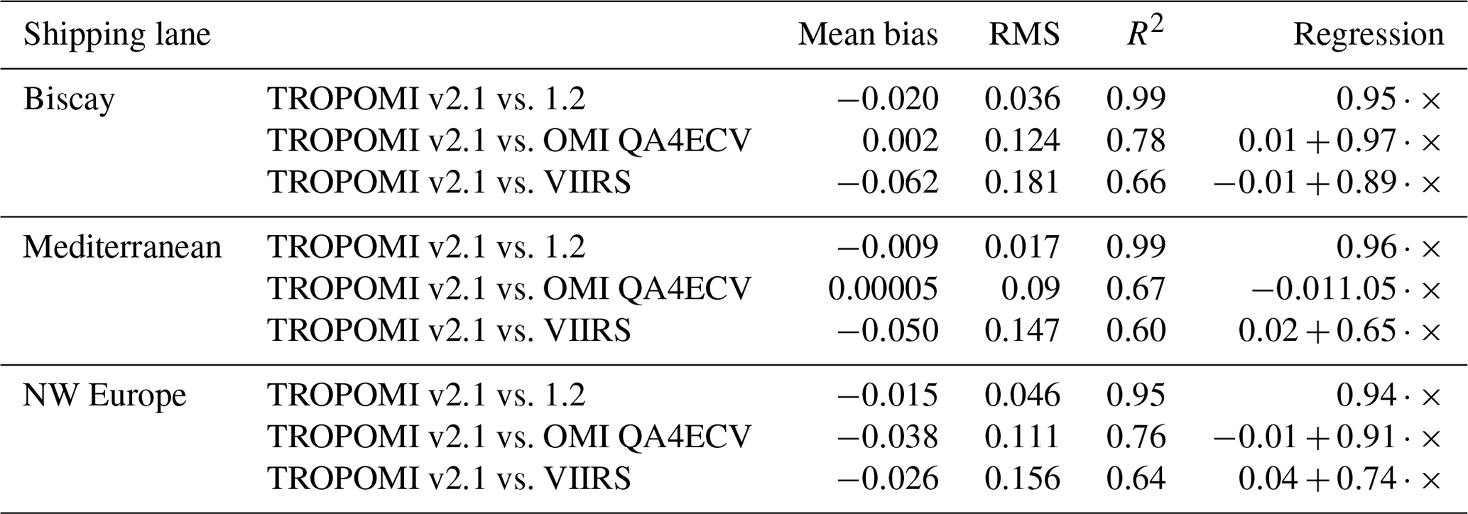
FRESCO+ wide cloud pressures are a clear improvement over the FRESCO+ data used in v1.2–1.3. Figure 6 shows a comparison of gridded, co-sampled cloud pressure distributions from TROPOMI v1.2 (FRESCO+), TROPOMI v2.1 (FRESCO+ wide), OMI QA4ECV, and VIIRS over the Bay of Biscay between 1 and 7 July 2018. As expected, the improved TROPOMI v2.1 cloud pressures are ≈40 hPa lower than for v1.2, in line with their enhanced sensitivity, and show more realistic, elevated clouds. It is apparent that OMI cloud pressures are generally lower and show a flatter distribution than the other products. TROPOMI v2.1 and v1.2 show similar distributions as VIIRS, with v1.2 pressures higher by 50 hPa in the median and v2.1 moving closer to VIIRS with a difference of 2 hPa relative to VIIRS. We find similar agreement between TROPOMI and independent data over the Mediterranean Sea and Northwest Europe as shown in Table D2. FRESCO+ wide cloud pressures agree best but remain higher than VIIRS in the median (both FRESCO cloud pressure distributions show a larger tail towards low pressures compared to VIIRS, possibly caused by filtering for liquid water clouds in VIIRS). This is in line with expectations as VIIRS's infrared cloud retrieval is mostly sensitive to the cloud top (Platnick et al., 2017), whereas FRESCO’s O2–A band retrieval is more sensitive to the center of a cloud (e.g., Sneep et al., 2008). Around 25 %–30 % of VIIRS cloud retrievals in the areas studied here are ice water clouds and therefore not included in the analysis. As these clouds appear at higher altitudes, improved cloud pressures have only a little influence on the NO2 columns (see Sect. 3.3.3).
Table 3Evaluation of TROPOMI v2.1 cloud pressures against reference data for the Bay of Biscay.
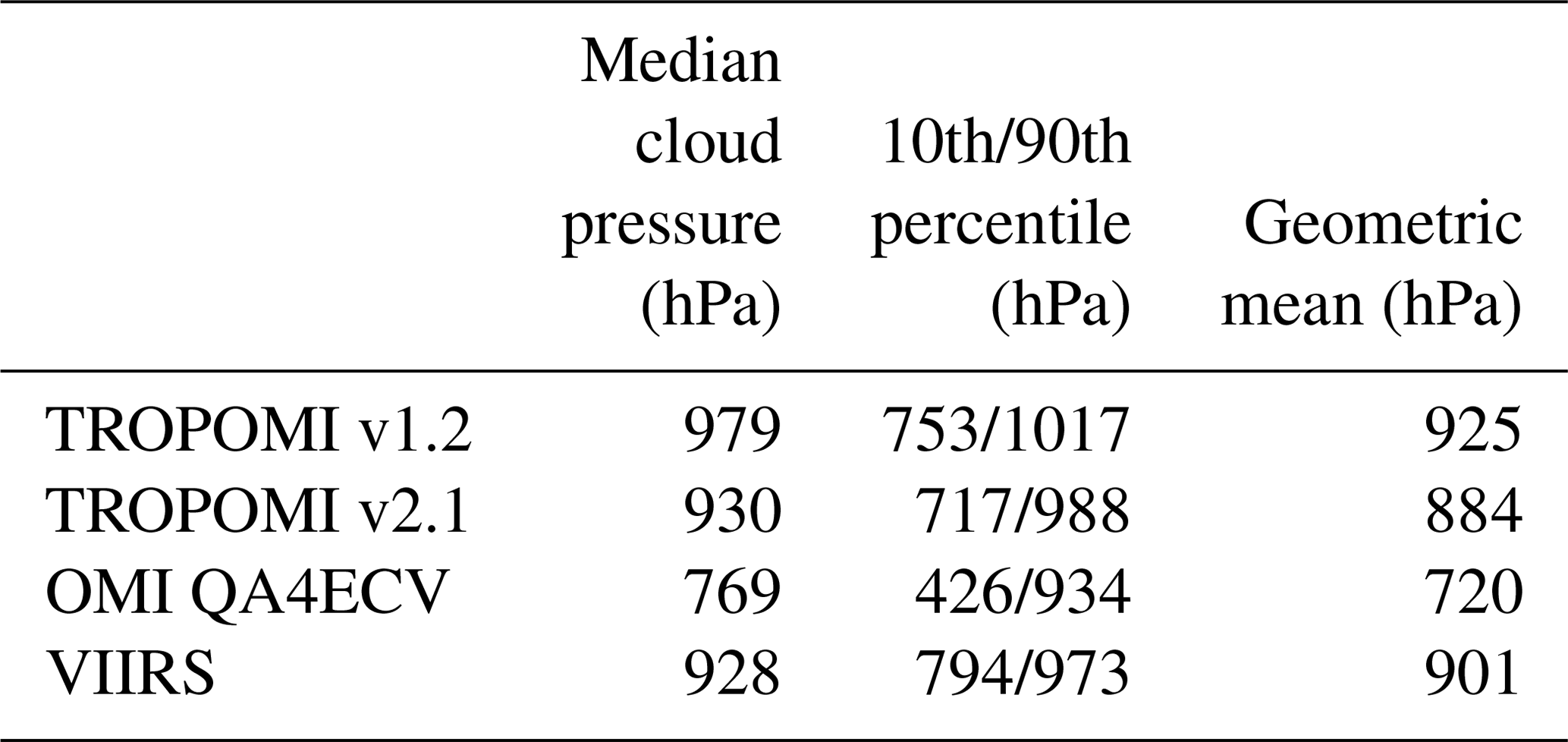
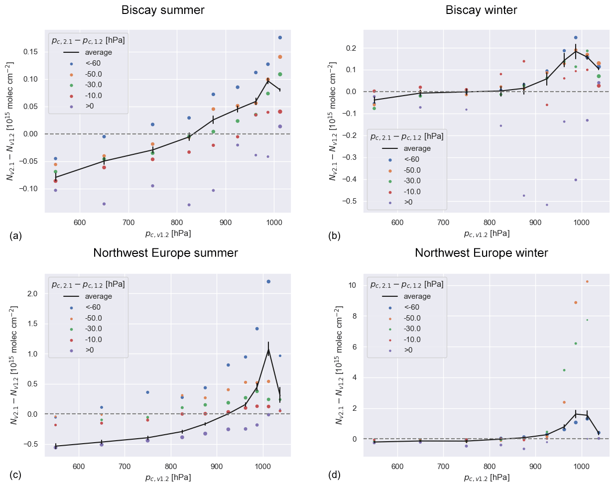
Figure 7Difference between tropospheric NO2 columns retrieved with TROPOMI v1.2 and v2.1 as a function of the v1.2 cloud pressure for 27 June–6 July 2018 over the mildly polluted Bay of Biscay in summer (a) and winter (b), as well as the highly polluted Northwest Europe (c, d). Colors indicate the difference in cloud pressures between the two versions. The marker size is proportional to the logarithm of the sample size, and the black line shows the effective average.
3.3.3 Effect of improved cloud pressure on TROPOMI NO2 columns
The improved cloud pressures lead to increases in NO2 columns of up to 40 % depending on area and season. The left panels of Fig. 7 show the change in tropospheric NO2 columns as a function of cloud pressure over the Bay of Biscay and Northwest Europe in summer. We see that NO2 columns increase most for locations that had the highest original v1.2 cloud pressures and that the improvements are strongest when cloud pressures are reduced most (light blue dots). The increase over the Bay of Biscay is smaller (up to 0.1×10¹⁵ molec. cm−2) than over Northwest Europe (up to 1.0×10¹⁵ molec. cm−2), reflecting the higher pollution levels over the mainland. We see similar patterns with stronger improvements in winter, as shown in the right panels of Fig. 7. The increased v2.1 NO2 columns indicate that the v1.2 TROPOMI NO2 product suffers from a “cloud shielding” effect: NO2 columns are underestimated due to clouds that are situated too low within the polluted boundary layer, and improved v2.1 cloud pressures (at least partly) resolve the low bias in v1.2 NO2 columns. For this analysis, we compared the TROPOMI v2.1 columns retrieved with improved cloud information to the TROPOMI v1.2 NO2 columns. We used 10 d in four different seasons (27 June–6 July 2018, 28 December 2018–5 January 2019, 25 March–5 April 2019, and 13–23 September 2019) for which both v2.1 test data and v1.2 operational data were available to us as part of the DDS-2B. Our comparison focused on mostly clear-sky situations (fc<0.2), which are most relevant for the detection of near-surface pollution sources.
We trained a deep neural network (DNN) to predict v2.1 columns for the full TROPOMI mission period up to December 2020 and thereby created a consistent data set. The DNN-predicted v2.1 (hereafter v2.1p) reduces the mean difference to the retrieved v2.1 NO2 columns to molec. cm−2 (original v2.1–v1.2 mean difference was 0.12×10¹⁵ molec. cm−2) over the three areas (see Sect. 2.2) of study during the four periods, suggesting considerable skill in the DNN approach. Details can be found in Appendix E.
Figure 8 shows the averaged NO2 columns from v2.1p over the summer of 2019 and winter of 2019/2020. The difference map in the right panels indicates that predicted v2.1 NO2 columns are higher by up to 0.5×10¹⁵ molec. cm−2, especially over the most polluted seas such as the English Channel and shipping lanes. We find a stronger impact of the improved cloud pressures in the winter season, reflecting that NO2 pollution is confined in a thinner marine boundary layer in that season.
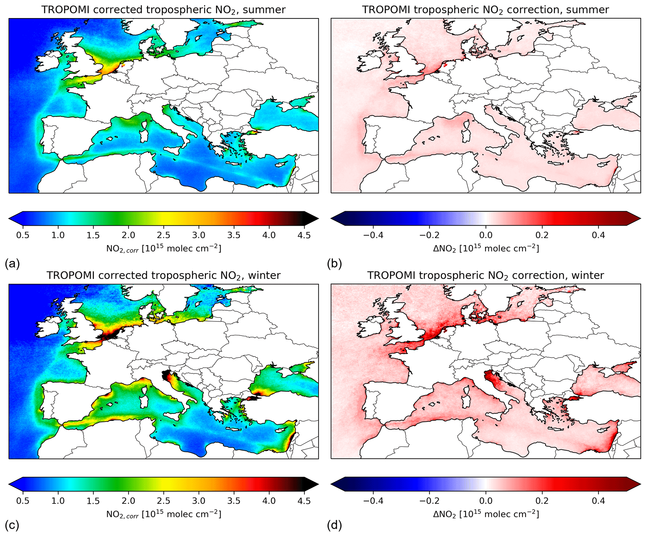
Figure 8Effect of DNN correction: (a) corrected TROPOMI data for summer (May–September) 2019, (b) change in NO2 columns by the correction for the same period (v2.1p–v1.3), (c) corrected TROPOMI data for winter (November–April) 2019/2020, and (d) change in NO2 columns by the correction for the same period (v2.1p–v1.3). Land areas are whitened out for clarity.
3.4 Comparison of TROPOMI and OMI NO2 columns in shipping lanes
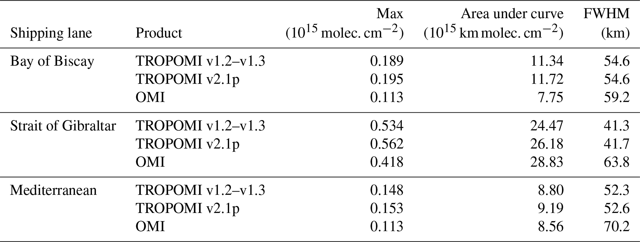
TROPOMI detects a more pronounced and narrower region of ship NO2 pollution than OMI. On average, TROPOMI v2.1p detects 45 % higher peak NO2 values than OMI. TROPOMI data allow the attribution of 14 % more NO2 to shipping lane enhancements and over 23 % to narrower shipping lanes. To quantitatively investigate TROPOMI's capability to detect NO2 over shipping lanes under different measurement conditions and compare it to OMI's, we created average NO2 cross sections over busy shipping lanes. We studied NO2 enhancements in summer 2019 (June–August) over shipping lanes in the Bay of Biscay, from Sicily to the Suez Canal, and east of Gibraltar, the regions visually defined in Fig. 1c. First, we defined the location of the shipping lanes according to the emission data shown in Fig. 1c. Then, we calculated the average NO2 columns along the shipping lane and parallel to it, taking care to exclude NO2 columns measured over land. In that way we created an average cross section of NO2 over shipping lanes. In the last step, we performed a background correction by subtracting a linear NO2 background to isolate the NO2 enhancements caused by shipping. The orbital data were gridded to regular grids of 0.0625∘ × 0.0625∘ and 0.125∘ × 0.125∘ resolution for TROPOMI and OMI, respectively. For TROPOMI only pixels with fQA>0.75 were taken into account. For OMI, a consistent filtering was applied, including maximal solar and viewing zenith angles of 80∘ and maximal cloud radiance fractions of 0.5. The resulting cross sections are shown in Fig. 9. Table 4 summarizes the peak value, the area under the curve (i.e., the total NO2 attributed to shipping) and the full width at half maximum (FWHM) for the three shipping lanes. It should be noted that the grid used for OMI is 2 times coarser than the one used for TROPOMI. Gridding TROPOMI to the coarser grid used for OMI only changes the results slightly, indicating that the improved spatial resolution of TROPOMI indeed improves the detection of NO2 from narrow ship lanes and is in line with the finding of new shipping lanes shown in Fig. 2.

Figure 9Mean enhancement cross sections in June–August 2019. TROPOMI v1.2–v1.3 in black, the improved TROPOMI v2.1p in green, and OMI in grey. Shaded areas indicate the 95 % confidence interval.
As already seen in Fig. 8, the v2.1p data set shows slightly higher NO2 compared to the TROPOMI v1.2–v1.3 data, especially in the center of the lane, while background NO2 is less affected by the correction. The impact of the DNN is larger in winter than in summer as discussed before.
Table 4Statistics for the NO2 enhancement cross section over the Mediterranean shipping lane.
For the Bay of Biscay it is also apparent that the NO2 peak is shifted to the east for all data sets. As the location is defined by an emission inventory based on AIS data (and therefore real ship location), this is likely an effect of dominant westerly winds.
We conclude that TROPOMI provides a significant improvement for the detection of shipping NO2 with sharper and more pronounced shipping lanes in seasonal averages. The improved v2.1p TROPOMI data increase the signal further.
3.5 Reductions in ship NOx emissions during the COVID-19 pandemic
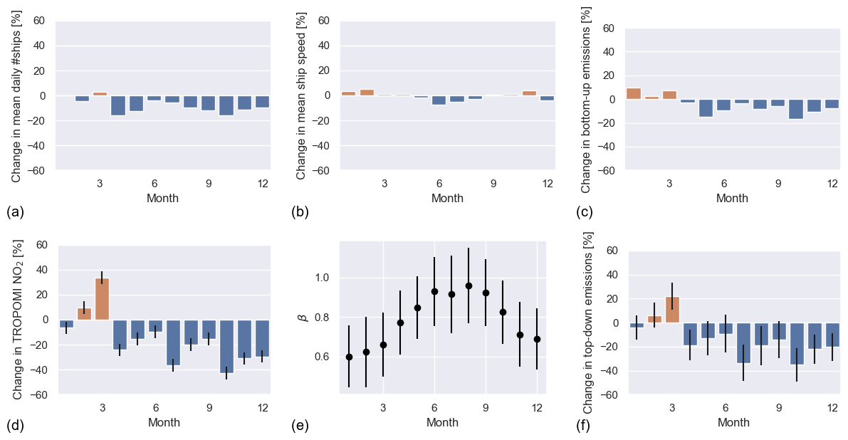
Figure 10(a) Relative change in monthly mean of daily number of ships passing the Strait of Gibraltar between 2019 and 2020 inferred from AIS data. (b) Same but with average ship speed. (c) Relative change in emission proxy (v3⋅L2). (d) Relative change in TROPOMI shipping NO2. (e) Monthly β values from Vinken et al. (2014b) with month-to-month variability imposed by monthly values from Verstraeten et al. (2015). Uncertainty intervals represent the temporal and spatial variability in β (see discussion in the text). (f) Relative change in top-down emissions from shipping. Error bars represent the propagated uncertainties in TROPOMI shipping NO2, β, and differences in meteorological conditions between 2019 and 2020 (see discussion in the text).
Emission proxies derived from AIS data and from TROPOMI NO2 suggest emission reductions from shipping in 2020 compared to 2019 as depicted in Fig. 10c and f. While in the first 3 months of 2020 the ship emissions were generally higher compared to 2019, both emission proxies show reductions starting in April and lasting until the end of the year. This reduction can be linked to the COVID-19 pandemic, which led to economic lockdowns in many countries of the world. Europe had its most stringent measures in spring and autumn 2020.
We created daily 0.0625×0.0625∘ maps of TROPOMI data using v2.1p NO2 columns as described in Sect. 3.3.3 with fQA≥0.75. We calculate the area under the cross section as a measure for shipping NO2 for monthly mean NO2 columns for the shipping lanes of Gibraltar and the Mediterranean defined in Fig. 1c. Monthly TROPOMI shipping NO2 for 2019 and 2020 can be seen in Fig. S2c. Figure 10d shows the relative change in shipping NO2 from 2019 to 2020 in the Strait of Gibraltar. Using β values and the approach described Sect. 2.4 and shown in Fig. 10e, we arrive at the TROPOMI-based relative change in emission changes shown in Fig. 10f.
The uncertainty in our top-down NOx emission changes follows from the following: (i) the sensitivity of TROPOMI shipping NO2 to the area of study (σarea=5 %), (ii) the inter-year differences on monthly averaged NO2 columns over the areas of study caused by meteorology, and (iii) the combined spatial and temporal spread of β as a result of differences in the chemical regime caused, for example, by differences in atmospheric composition and radiation (σβ=0.15). Figures 10d and F1d show σarea, in panel (e) uncertainties (ii) and (iii) are used, while for panel (f) a full error propagation of all uncertainties listed above was performed. A full discussion on the uncertainty estimates can be found in Sect. S4.
Additionally, we used AIS data to calculate an AIS-based emission proxy as described in Sect. 2.5. We filtered for days with TROPOMI coverage of at least 50 % of each study area. AIS data indicate that the number of ships passing per month through the Strait of Gibraltar has reduced from March 2020 onwards relative to 2019 (Figs. 10a and S2a). The average speed of the ships passing through the shipping lanes is lower between May–September 2020 compared to the same period in 2019 as well (Figs. 10b and S2b). This is in agreement with a study by Millefiori et al. (2020) who found an increase in container ship speed in May and June in 2019 which is absent in 2020 leading to a relative decrease. Finally, Fig. 10c shows the relative change in AIS-deduced emission proxy from 2019 to 2020. Similar results for the shipping lane in the Mediterranean can be found in Figs. F1 and S3.
Several studies report changes in ship activity in 2020 using AIS data. In addition to the 5 % decrease in ship speed in the Mediterranean between March and April 2020 compared to 2019 mentioned above, Millefiori et al. (2020) reported global mobility of container ships to have decreased by 10 % between March and June 2020 compared to the previous year. March et al. (2021) find increases in traffic density for January and February 2020 with decreases in March–June, with western Europe showing very strong reductions. Both studies show strong variations by vessel category and geographical distribution. Doumbia et al. (2021) find a global decrease in container ship port calls in 2020 of 7 %, with a monthly local reduction of 20 % for Europe in June. The timing and magnitude of reductions reported in these studies agree with our findings: on average, AIS data indicate a reduction of 9 % (2 %) in April–December for Gibraltar (Mediterranean). The TROPOMI-based emission estimates agree in timing but show larger magnitude in reduction (20 % and 10 %) in April–December for the shipping lanes in the Strait of Gibraltar and the Eastern Mediterranean, respectively.
While the top-down emission reductions show a larger magnitude compared to the bottom-up emissions, they largely agree within the margin of uncertainty on a month-to-month basis. The difference in the mean reduction magnitude might be due to chemistry. The β values used here are calculated on a coarse grid (0.5∘ × 0.67∘). Additionally, we assume the chemical conditions in 2019 and 2020 to be similar to 2006 for when the β values were calculated. Furthermore, lateral transport complicates the choice of NO2 background as a discrimination between land and ship emissions is not possible. The NO2 background in turn has a large influence on the top-down emission estimate. These factors are all considered in our uncertainty estimates of the top-down emission changes. Other possible sources of uncertainty lie in the different temporal and spatial sampling of AIS and TROPOMI data and the simplified emission proxy. However, this is not expected to lead to a systematic bias.
We used tropospheric NO2 column observations from the TROPOMI sensor to optimally monitor ship NO2 pollution and study the changes in ship NOx emissions over European seas in 2019–2020. Satellite observations of tropospheric NO2 columns provide valuable information on ship air pollution over open seas, which can be used to inform compliance monitoring by flag states and national authorities. We evaluated the high-resolution TROPOMI NO2 retrievals for its potential to better detect ship NO2 pollution. In European waters alone, TROPOMI finds six new lanes with enhanced NO2 ranging from the Aegean Sea to the Skagerrak between Denmark and Norway, which are not detected by OMI and which have not previously been reported in the literature. These newly found lanes of pollution coincide with busy sailing routes and bottom-up emission proxies.
To better understand the recent detection of an individual ship’s NO2 plume under conditions of sun glint, we examined how sun glint viewing geometries affect subsequent steps in the TROPOMI retrieval procedure. We find that sun glint drives higher apparent scene reflectivity, which enhances the signal strength from spectral fitting of NO2 columns along the average light path by 20 %–30 % over clear-sky shipping lanes. In such situations, the vertical sensitivity to NO2 within the marine boundary layer increases by up to 60 %. This effect is especially strong when sea surface wind speeds are low but non-zero. When winds are strong, the wash causes sunlight to be reflected in other directions than directly towards the satellite, leading to little gain in vertical sensitivity. We find that the TROPOMI NO2 algorithm accounts for these effects so that data within and outside of sun glint geometries can be used with confidence. Nevertheless, our work clearly indicates that optimal spectral fitting can be accomplished for small scattering angles (<15∘) and sea surface wind speeds of 1.5–3 m s−1. Although selecting a subset fulfilling these sampling criteria reduces the amount of available data sharply, our findings indicate that sun glint conditions are beneficial for quantifying previously undetectable small NOx emission sources over open sea and holding promise for also detecting other trace gases with UV–Vis satellite instruments over water, where surface reflectivity and vertical sensitivity are generally small.
In November 2020, KNMI implemented an improved FRESCO+ cloud retrieval called FRESCO+ wide in the operational TROPOMI NO2 algorithm. We find here that this new FRESCO+ wide cloud retrieval provides some 50 hPa lower cloud pressures which agree better with coinciding cloud top heights from the VIIRS sensor than the standard FRESCO+. We show that the improved cloud pressures lead to a more realistic description of vertical sensitivities in the TROPOMI NO2 algorithm and at least partly address the known low bias in the tropospheric NO2 product prior to November 2020, thus not only solving a known issue in the TROPOMI NO2 retrieval but also increasing signal strength. We then trained a neural network on a limited data set of simultaneously available standard and improved cloud and NO2 retrievals. Based on four different training sets, the neural network learned the statistical relationship between standard FRESCO+ cloud pressures and other parameters and the new tropospheric NO2 columns. We used the neural network to predict updated NO2 columns for the entire 2019–2020 TROPOMI NO2 record. The neural network predicts a general increase in tropospheric NO2 columns. Increases are particularly strong (up to 4×10¹⁵ molec. cm−2) in the most polluted regions of Europe in wintertime. Our predicted (v2.1p) TROPOMI data set enables the consistent analysis of temporal changes in NO2 during the COVID year 2020 and is useful to other data users until the TROPOMI NO2 reprocessing scheduled for 2022 has been completed.
We compared changes in our v2.1p TROPOMI NO2 columns between 2019 and 2020 to changes in the number of ships, their speed, and their size obtained from AIS data in the main European traffic lanes. From April 2020 onwards, TROPOMI observes 25 % less NO2 pollution than in the year before, in step with a 10 % reduction in the number of ships and a 5 % speed reduction relative to 2019. Accounting for non-linearity in local NOx chemistry, we infer an average 20 % reduction in top-down NOx emissions in the Strait of Gibraltar from ships during months in which COVID measures were in force in Europe, and global mobility decreased as a result of the pandemic. For future research, a full chemical transport modeling of AIS-based emissions and strict co-sampling of AIS and TROPOMI data can help with understanding the observed differences in top-down and bottom-up emission changes and reduce the error margins.
We showed that TROPOMI is a superior instrument to analyze relatively small enhancements in NO2 pollution over dark European seas. Its vertical sensitivity to ship pollution is substantially enhanced for small scattering angles under cloud free conditions and low wind speeds. Such sun glint scenes should allow improved detection of other pollutants, such as formaldehyde and SO2 as well. KNMI's operational TROPOMI NO2 product is subject to continuous improvement, which causes step changes in the publicly available data record until the official reprocessing has been finalized. Our improved (v2.1p) TROPOMI data set offers a consistent alternative that can be used over Europe in and after 2019 and may be applied to other regions of the world where consistent NO2 time series are needed.
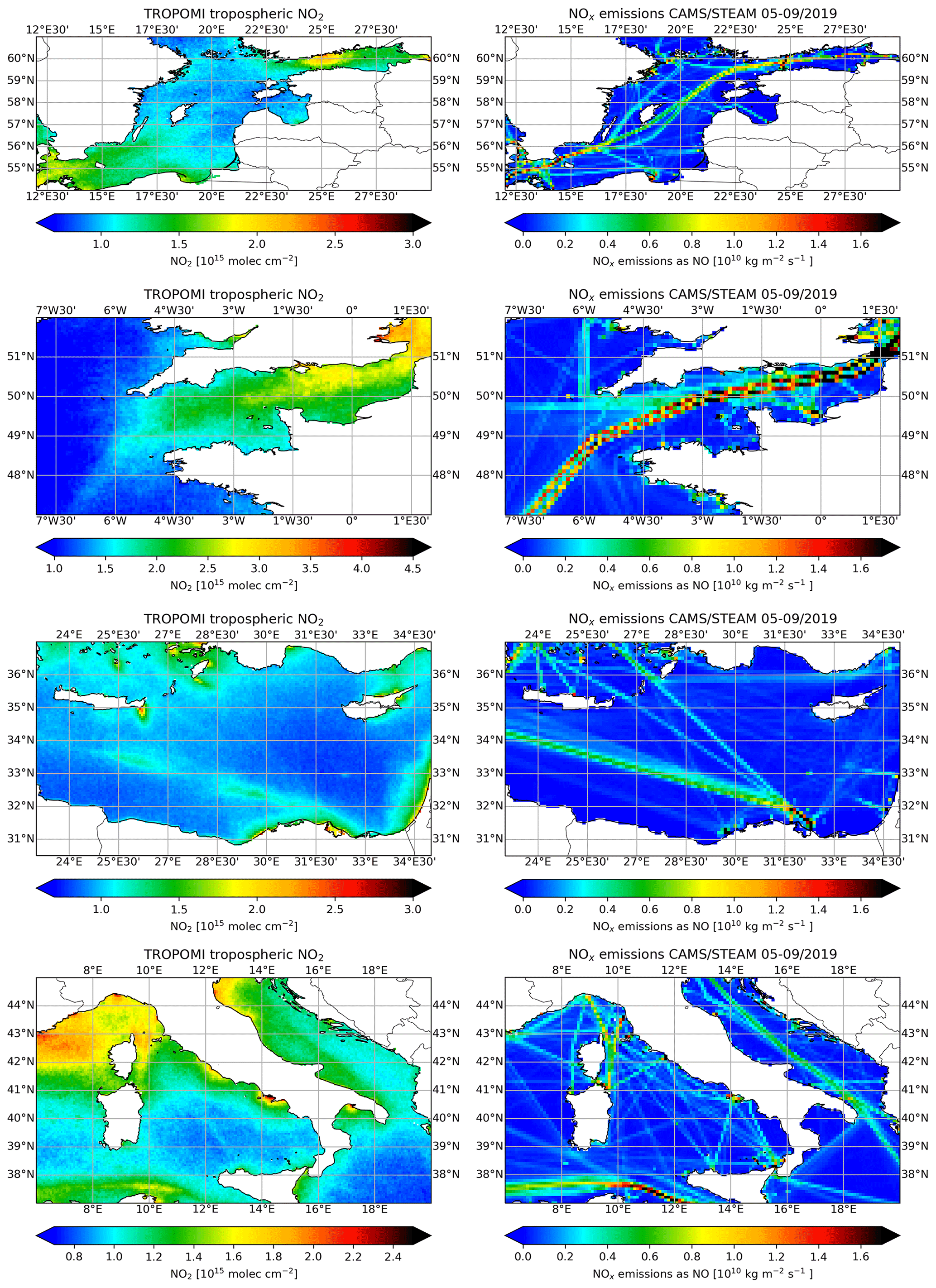
Figure A1Summertime mean (May–September) tropospheric NO2 columns from TROPOMI (left panels) and summertime mean NOx emissions from the CAMS/STEAM emission inventory (right panels; Granier et al., 2019; Johansson et al., 2017).
We calculate a geometric tropospheric vertical column density Ntrop,geo using
where Ns,trop is the tropospheric slant column density which can be calculated from the TROPOMI files using
where M, Ns, and Nv are mean air mass factor, slant column density, and vertical column density, respectively. The subscripts trop, tot, and strat indicate tropospheric, total, and stratospheric columns, respectively. Mgeo can be calculated using the solar zenith angle θ and the viewing zenith angle θ0 as . The resulting tropospheric column is shown in Fig. B1.
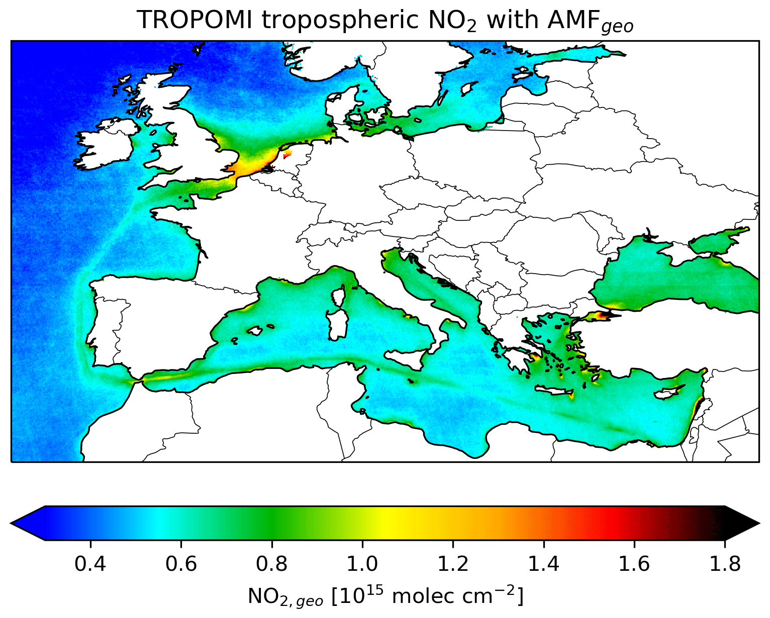
Figure B1Mean of NO2 columns calculated with geometrical AMF for summer 2019 (May–September); land areas have been whitened for clarity.
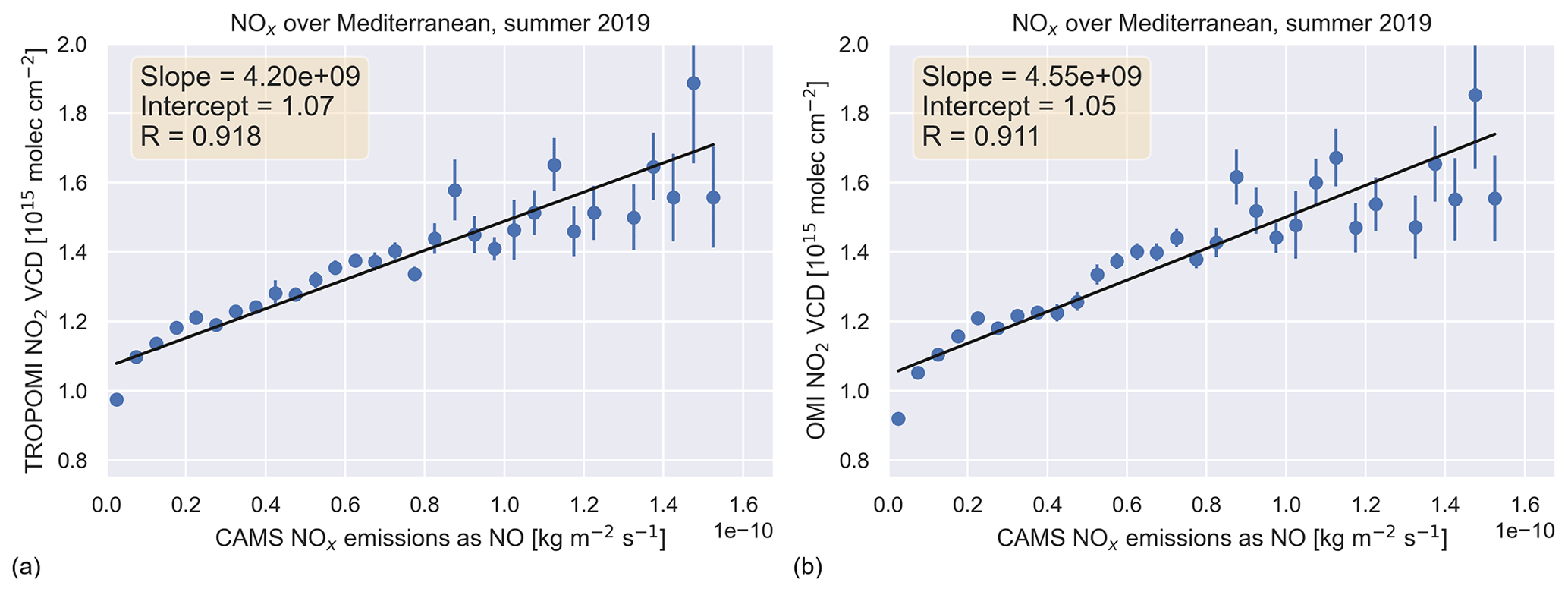
Figure C1Scatter of binned summertime (May–September) 2019 tropospheric NO2 columns vs. emissions from CAMS/STEAM for the same period at 0.1∘ × 0.1∘ in the Mediterranean. Error bars indicate the standard error of the bin. (a): TROPOMI; (b): OMI.
Table D1Evaluation of TROPOMI v2.1 cloud fractions over European shipping lanes (1–6 July 2018) against reference data.
D1 Cloud fractions
The improved (v2.1) and old (v1.2) cloud fractions have a strong correlation (R2=0.99), but v2.1 cloud fractions are 5 % lower on average; see Table D1. The spatiotemporal correlation between TROPOMI v2.1 and the well-established OMI QA4ECV cloud fraction product is also very high (R2=0.78), with TROPOMI v2.1 cloud fractions 3 % lower than OMI on average. TROPOMI v2.1 shows high correlation (R2=0.66) and somewhat lower cloud fractions (−11 %) compared to the co-sampled effective VIIRS cloud fractions. TROPOMI cloud fractions are especially lower for partly cloud-covered scenes, possibly resulting from biased surface albedos assumed in the TROPOMI retrieval (from the GOME-2 climatology at 0.5∘ resolution, see Table 1). We find a similar high correlation and small differences between TROPOMI and independent data over the Mediterranean Sea and Northwest Europe as shown in Table D1.
D2 Cloud pressures
Table D2Evaluation of TROPOMI v2.1 cloud pressures against reference data for European shipping lanes.

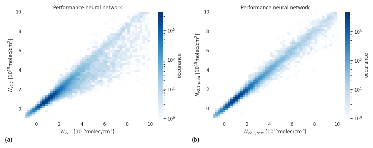
Figure E1(a) Scatterplot of TROPOMI v1.2 (uncorrected) vs. actually retrieved v2.1 TROPOMI NO2 columns observed over Europe in the four test periods. (b) Scatterplot of DNN-predicted vs. actually retrieved v2.1 TROPOMI NO2 columns observed over Europe in all areas and periods under study.
An artificial neural network allows us to predict v2.1 columns for the full TROPOMI mission period up to December 2020. We find the predicted v2.1 columns to be close to actual retrieved v2.1 columns in a testing data set. Figure E1 illustrates the skill of the DNN approach to reliably predict v2.1 data: as a reduced major axis regression shows, the DNN-predicted v2.1 (hereafter v2.1p) NO2 columns agree substantially better with the retrieved v2.1 NO2 values ( molec. cm−2, R2=0.98, n=56219) compared to the originally retrieved v1.2 NO2 columns ( molec. cm−2, R2=0.91). The improvement from TROPOMI v1.2 to v2.1 is driven by the improved cloud pressures and associated changes in the tropospheric AMFs.
We trained the artificial DNN using the Python package Keras (Chollet and others, 2015) with three hidden layers. We divided the combined v1.2 and v2.1 data sets in three random subsets for training (60 %), validation (20 %), and testing (20 %). The input parameters to predict TROPOMI (pseudo) v2.1 NO2 columns are Nv,v1.2, Mtrop, fcl, pcl, all viewing geometry parameters, surface albedo, and the fQA value (all from v1.2). The DNN was then trained to minimize the mean absolute difference between the predicted and actually retrieved v2.1 NO2 columns from the training set. This means our prediction does not use FRESCO+ wide cloud pressures for dates outside the training set period. Rather, the DNN has been trained to predict new NO2 columns based on the old FRESCO+ cloud pressures and other parameters. Our DNN application succeeds in reducing the mean difference between the predicted and retrieved v2.1 NO2 columns to molec. cm−2 (original v2.1–v1.2 mean difference was 0.12×10¹⁵ molec. cm−2) over the three areas of study during the four periods, suggesting considerable skill in the DNN approach. Our improved data set consists of the original L2 TROPOMI NetCDF files with the predicted change in tropospheric NO2 columns as additional variable.
To show that DNN is capable of capturing seasonal variations in NO2 corrections and, more broadly, that we can use a generic DNN to correct historic TROPOMI v1.2 data, we train a DNN based on three seasons (summer, winter, and spring) and tested its predicted NO2 columns against actually retrieved v2.1 data in autumn. This analysis is done for the three testing areas defined in Sect. 3.3. After application of DNN, the mean discrepancy between predicted and retrieved v2.1 NO2 columns reduces to molec. cm−2 (original mean discrepancy: 0.09×10¹⁵ molec. cm−2), and R2 improved from 0.82 to 0.97.
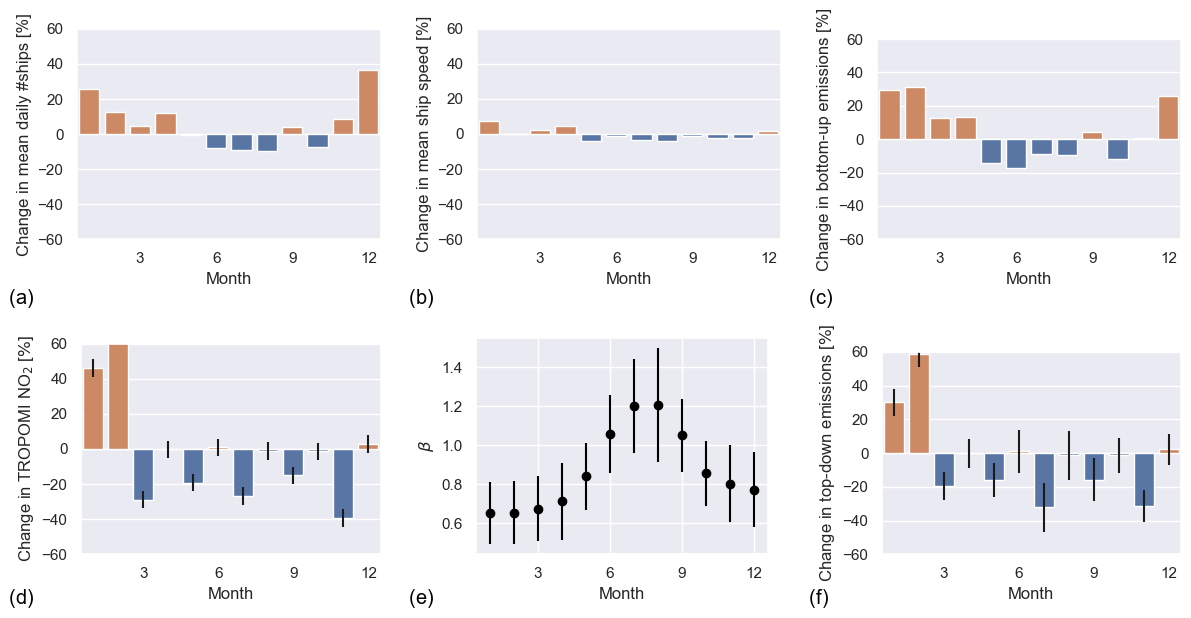
Figure F1(a) Relative change in monthly mean of daily number of ships passing the Mediterranean shipping lane between 2019 and 2020. (b) Same but with average ship speed. (c) Relative change in emission proxy (v3⋅L2). (d) Relative change in TROPOMI shipping NO2; the error bars indicate the sensitivity to changes in the area of study. (e) Monthly β values as discussed in Sect. 2.4. Error bars represent uncertainty originating from the temporal and spatial variability (see discussion in the text). (f) Relative change in top-down emissions from shipping. Error bars represent the propagated uncertainties in TROPOMI shipping NO2, β, and differences in meteorological conditions between 2019 and 2020 (see discussion in the text).
The data can be made available upon request by contacting the author (christoph.riess@wur.nl). TROPOMI L2 NO2 is publicly available via the Copernicus open-access hub (https://s5phub.copernicus.eu/dhus/#/home, van Geffen et al., 2019).
The supplement related to this article is available online at: https://doi.org/10.5194/amt-15-1415-2022-supplement.
TCVWR, KFB, and JvV designed the study. TCVWR performed the data analysis with support from KFB, JvV, and WP. TCVWR wrote the manuscript with contributions from KFB, JvV, and WP. JvV made the AIS data available. MS developed the FRESCO+ wide algorithm, and JvG provided specifics on the TROPOMI NO2 data versions and made the DDS-2B available. HE oversees the NO2 retrieval improvements at KNMI. All authors reviewed the manuscript.
The contact author has declared that neither they nor their co-authors have any competing interests.
Publisher’s note: Copernicus Publications remains neutral with regard to jurisdictional claims in published maps and institutional affiliations.
The authors want to thank Auke van der Woude for his help regarding the neural network.
This work is funded by the Netherlands Human Environment and Transport Inspectorate and the Dutch Ministry of Infrastructure and Water Management.
This research has been supported by the Horizon 2020 (SCIPPER (grant no. 814893)).
This paper was edited by Natalya Kramarova and reviewed by two anonymous referees.
Acarreta, J. R., De Haan, J. F., and Stammes, P.: Cloud pressure retrieval using the O2-O2 absorption band at 477 nm, J. Geophys. Res.-Atmos., 109, 1–11, https://doi.org/10.1029/2003jd003915, 2004.
Agrawal, H., Welch, W. A., Miller, J. W., and Cocker, D. R.: Emission measurements from a crude oil tanker at sea, Environ. Sci. Tech., 42, 7098–7103, https://doi.org/10.1021/es703102y, 2008.
Beirle, S., Platt, U., von Glasow, R., Wenig, M., and Wagner, T.: Estimate of nitrogen oxide emissions from shipping by satellite remote sensing, Geophys. Res. Lett., 31, 4–7, https://doi.org/10.1029/2004GL020312, 2004.
Beirle, S., Borger, C., Dörner, S., Li, A., Hu, Z., Liu, F., Wang, Y., and Wagner, T.: Pinpointing nitrogen oxide emissions from space, Sci. Adv., 5, 1–7, https://doi.org/10.1126/sciadv.aax9800, 2019.
Berg, N., Mellqvist, J., Jalkanen, J.-P., and Balzani, J.: Ship emissions of SO2 and NO2: DOAS measurements from airborne platforms, Atmos. Meas. Tech., 5, 1085–1098, https://doi.org/10.5194/amt-5-1085-2012, 2012.
Boersma, K. F., Eskes, H. J., and Brinksma, E. J.: Error analysis for tropospheric NO2 retrieval from space, J. Geophys. Res.-Atmos., 109, D4, https://doi.org/10.1029/2003jd003962, 2004.
Boersma, K. F., Jacob, D. J., Bucsela, E. J., Perring, A. E., Dirksen, R., van der A, R. J., Yantosca, R. M., Park, R. J., Wenig, M. O., Bertram, T. H., and Cohen, R. C.: Validation of OMI tropospheric NO2 observations during INTEX-B and application to constrain NOx emissions over the eastern United States and Mexico, Atmos. Environ., 42, 4480–4497, https://doi.org/10.1016/j.atmosenv.2008.02.004, 2008.
Boersma, K. F., Vinken, G. C., and Tournadre, J.: Ships going slow in reducing their NOx emissions: Changes in 2005–2012 ship exhaust inferred from satellite measurements over Europe, Environ. Res. Lett., 10, 74007, https://doi.org/10.1088/1748-9326/10/7/074007, 2015.
Boersma, K. F., Vinken, G. C. M., and Eskes, H. J.: Representativeness errors in comparing chemistry transport and chemistry climate models with satellite UV–Vis tropospheric column retrievals, Geosci. Model Dev., 9, 875–898, https://doi.org/10.5194/gmd-9-875-2016, 2016.
Boersma, K. F., van Geffen, J., Eskes, H., van der A, R., De Smedt, I., Van Roozendael, M., Yu, H., Richter, A., Peters, E., Beirle, S., Wagner, T., Lorente, A., Scanlon, T., Compernolle, S., and Lambert, J.-C.: Product Specification Document for the QA4ECV NO2 ECV precursor product, techreport QA4ECV Deliverable D4.6, KNMI, available at: http://www.qa4ecv.eu/sites/default/files/D4.6.pdf (last access: 2 February 2022), 2017.
Boersma, K. F., Eskes, H. J., Richter, A., De Smedt, I., Lorente, A., Beirle, S., van Geffen, J. H. G. M., Zara, M., Peters, E., Van Roozendael, M., Wagner, T., Maasakkers, J. D., van der A, R. J., Nightingale, J., De Rudder, A., Irie, H., Pinardi, G., Lambert, J.-C., and Compernolle, S. C.: Improving algorithms and uncertainty estimates for satellite NO2 retrievals: results from the quality assurance for the essential climate variables (QA4ECV) project, Atmos. Meas. Tech., 11, 6651–6678, https://doi.org/10.5194/amt-11-6651-2018, 2018.
Buriez, J.-C.: An improved derivation of the top-of-atmosphere albedo from POLDER/ADEOS-2: Narrowband albedos, J. Geophys. Res., 110, D05202, https://doi.org/10.1029/2004JD005243, 2005.
Chen, G., Huey, L. G., Trainer, M., Nicks, D., Corbett, J., Ryerson, T., Parrish, D., Neuman, J. A., Nowak, J., Tanner, D., Holloway, J., Brock, C., Crawford, J., Olson, J. R., Sullivan, A., Weber, R., Schauffler, S., Donnelly, S., Atlas, E., Roberts, J., Flocke, F., Hübler, G., and Fehsenfeld, F.: An investigation of the chemistry of ship emission plumes during ITCT 2002, J. Geophys. Res.-Atmos., 110, 1–15, https://doi.org/10.1029/2004JD005236, 2005a.
Chen, G., Huey, L. G., Trainer, M., Nicks, D., Corbett, J., Ryerson, T., Parrish, D., Neuman, J. A., Nowak, J., Tanner, D., Holloway, J., Brock, C., Crawford, J., Olson, J. R., Sullivan, A., Weber, R., Schauffler, S., Donnelly, S., Atlas, E., Roberts, J., Flocke, F., Hübler, G., and Fehsenfeld, F.: An investigation of the chemistry of ship emission plumes during ITCT 2002, J. Geophys. Res.-Atmos., 110, 1–15, https://doi.org/10.1029/2004JD005236, 2005b.
Chollet, F., Bursztein, E., Jin, H., Watson, M., and Zhu, Q. S.: Keras, https://github.com/fchollet/keras (last access: 21 December 2021), 2015.
Compernolle, S., Argyrouli, A., Lutz, R., Sneep, M., Lambert, J.-C., Fjæraa, A. M., Hubert, D., Keppens, A., Loyola, D., O'Connor, E., Romahn, F., Stammes, P., Verhoelst, T., and Wang, P.: Validation of the Sentinel-5 Precursor TROPOMI cloud data with Cloudnet, Aura OMI O2–O2, MODIS, and Suomi-NPP VIIRS, Atmos. Meas. Tech., 14, 2451–2476, https://doi.org/10.5194/amt-14-2451-2021, 2021.
Corbett, J. J., Winebrake, J. J., Green, E. H., Kasibhatla, P., Eyring, V., and Lauer, A.: Mortality from ship emissions: A global assessment, Environ. Sci. Technol., 41, 8512–8518, https://doi.org/10.1021/es071686z, 2007.
Cox, C. and Munk, W.: Slopes of the sea surface deduced from photographs of sun glitter, Bulletin of the scripps institution of oceanography of the University of California, 6, 401–488, 1956.
Crippa, M., Guizzardi, D., Muntean, M., Schaaf, E., Dentener, F., van Aardenne, J. A., Monni, S., Doering, U., Olivier, J. G. J., Pagliari, V., and Janssens-Maenhout, G.: Gridded emissions of air pollutants for the period 1970–2012 within EDGAR v4.3.2, Earth Syst. Sci. Data, 10, 1987–2013, https://doi.org/10.5194/essd-10-1987-2018, 2018.
Curier, R. L., Kranenburg, R., Segers, A. J., Timmermans, R. M., and Schaap, M.: Synergistic use of OMI NO2 tropospheric columns and LOTOS-EUROS to evaluate the NOx emission trends across Europe, Remote Sens. Environ., 149, 58–69, https://doi.org/10.1016/j.rse.2014.03.032, 2014.
de Haan, J., Bosma, P., and Hovenier, J.: The adding method for multiple scattering calculations of polarized light, Astron. Astrophys. (Berlin. Print), 183, 371–391, 1987.
De Ruyter de Wildt, M., Eskes, H., and Boersma, K. F.: The global economic cycle and satellite-derived NO2 trends over shipping lanes, Geophys. Res. Lett., 39, 2–7, https://doi.org/10.1029/2011GL049541, 2012.
Ding, J., van der A, R. J., Eskes, H. J., Mijling, B., Stavrakou, T., van Geffen, J. H., and Veefkind, J. P.: NOx Emissions Reduction and Rebound in China Due to the COVID-19 Crisis, Geophys. Res. Lett., 47, 1–9, https://doi.org/10.1029/2020GL089912, 2020.
Dirksen, R. J., Boersma, K. F., Eskes, H. J., Ionov, D. V., Bucsela, E. J., Levelt, P. F., and Kelder, H. M.: Evaluation of stratospheric NO2 retrieved from the Ozone Monitoring Instrument: Intercomparison, diurnal cycle, and trending, J. Geophys. Res.-Atmos., 116, 1–22, https://doi.org/10.1029/2010JD014943, 2011.
Doumbia, T., Granier, C., Elguindi, N., Bouarar, I., Darras, S., Brasseur, G., Gaubert, B., Liu, Y., Shi, X., Stavrakou, T., Tilmes, S., Lacey, F., Deroubaix, A., and Wang, T.: Changes in global air pollutant emissions during the COVID-19 pandemic: a dataset for atmospheric modeling, Earth Syst. Sci. Data, 13, 4191–4206, https://doi.org/10.5194/essd-13-4191-2021, 2021.
Eskes, H., Van Geffen, J., Boersma, F., Eichmann, K.-U., Apituley, A., Pedergnana, M., Sneep, M., Veefkind, J. P., and Loyola, D.: Sentinel-5 precursor/TROPOMI Level 2 Product User Manual Nitrogendioxide, Royal Netherlands Meteorological Institute, version 4.0.2., p. 147, 2019.
Eskes, H. J. and Boersma, K. F.: Averaging kernels for DOAS total-column satellite retrievals, Atmos. Chem. Phys., 3, 1285–1291, https://doi.org/10.5194/acp-3-1285-2003, 2003.
European Environment Agency: Nitrogen oxides (NOx) Emissions, https://www.eea.europa.eu/data-and-maps/indicators/eea-32-nitrogen-oxides-nox-emissions-1%0Ahttps://www.eea.europa.eu/data-and-maps/indicators/eea-32-nitrogen-oxides-nox-emissions-1/assessment.2010-08-19.0140149032-3 (last access: 29 June 2021), 2019.
Eyring, V., Köhler, H. W., Lauer, A., and Lemper, B.: Emissions from international shipping: 2. Impact of future technologies on scenarios until 2050, J. Geophys. Res.-Atmos., 110, 183–200, https://doi.org/10.1029/2004JD005620, 2005.
Eyring, V., Isaksen, I. S., Berntsen, T., Collins, W. J., Corbett, J. J., Endresen, O., Grainger, R. G., Moldanova, J., Schlager, H., and Stevenson, D. S.: Transport impacts on atmosphere and climate: Shipping, Atmos. Environ., 44, 4735–4771, https://doi.org/10.1016/j.atmosenv.2009.04.059, 2010.
Georgoulias, A. K., Boersma, K. F., Van Vliet, J., Zhang, X., Van Der A, R., Zanis, P., and De Laat, J.: Detection of NO2 pollution plumes from individual ships with the TROPOMI/S5P satellite sensor, Environ. Res. Lett., 15, 124037, https://doi.org/10.1088/1748-9326/abc445, 2020.
Granier, C., Darras, S., Denier Van Der Gon, H., Jana, D., Elguindi, N., Bo, G., Michael, G., Marc, G., Jalkanen, J.-P., and Kuenen, J.: The Copernicus Atmosphere Monitoring Service global and regional emissions (April 2019 version), https://doi.org/10.24380/d0bn-kx16, 2019.
Griffin, D., Zhao, X., McLinden, C. A., Boersma, F., Bourassa, A., Dammers, E., Degenstein, D., Eskes, H., Fehr, L., Fioletov, V., Hayden, K., Kharol, S. K., Li, S. M., Makar, P., Martin, R. V., Mihele, C., Mittermeier, R. L., Krotkov, N., Sneep, M., Lamsal, L. N., ter Linden, M., van Geffen, J., Veefkind, P., and Wolde, M.: High-Resolution Mapping of Nitrogen Dioxide With TROPOMI: First Results and Validation Over the Canadian Oil Sands, Geophys. Res. Lett., 46, 1049–1060, https://doi.org/10.1029/2018GL081095, 2019.
Hassler, B., McDonald, B. C., Frost, G. J., Borbon, A., Carslaw, D. C., Civerolo, K., Granier, C., Monks, P. S., Monks, S., Parrish, D. D., Pollack, I. B., Rosenlof, K. H., Ryerson, T. B., von Schneidemesser, E., and Trainer, M.: Analysis of long-term observations of NOx and CO in megacities and application to constraining emissions inventories, Geophys. Res. Lett., 43, 9920–9930, https://doi.org/10.1002/2016GL069894, 2016.
Heidinger, A. and Li, Y.: Algorithm Theoretical Basis Document AWG Cloud Height Algorithm (ACHA), Tech. rep., NOAA NESDIS Center for Satellite Applications and Research, 60 pp., NESDIS, Silver Spring, USA, 2017.
IMO: Nitrogen oxides (NOx) – Regulation 13, https://www.imo.org/en/OurWork/Environment/Pages/Nitrogen-oxides-(NOx)-–-Regulation-13.aspx (last access: 15 April 2020), 2013.
International Maritime Organization (IMO): AIS transponders, https://www.imo.org/en/OurWork/Safety/Pages/AIS.aspx (last access: 24 February 2021), 2014.
Jacob, D. J.: Introduction to Atmospheric Chemistry, by Daniel Jacob (Harvard University), Princeton University Press, https://projects.iq.harvard.edu/files/acmg/files/edu_jacob_atmchem_problems_jan_2021.pdf (last access: 30 June 2021), 1999.
Johansson, L., Jalkanen, J. P., and Kukkonen, J.: Global assessment of shipping emissions in 2015 on a high spatial and temporal resolution, Atmos. Environ., 167, 403–415, https://doi.org/10.1016/j.atmosenv.2017.08.042, 2017.
Kleipool, Q. L., Dobber, M. R., de Haan, J. F., and Levelt, P. F.: Earth surface reflectance climatology from 3 years of OMI data, J. Geophys. Res.-Atmos., 113, 1–22, https://doi.org/10.1029/2008JD010290, 2008.
Koelemeijer, R. B., Stammes, P., Hovenier, J. W., and De Haan, J. F.: A fast method for retrieval of cloud parameters using oxygen a band measurements from the Global Ozone Monitoring Experiment, J. Geophys. Res.-Atmos., 106, 3475–3490, https://doi.org/10.1029/2000JD900657, 2001.
Lack, D. A., Corbett, J. J., Onasch, T., Lerner, B., Massoli, P., Quinn, P. K., Bates, T. S., Covert, D. S., Coffman, D., Sierau, B., Herndon, S., Allan, J., Baynard, T., Lovejoy, E., Ravishankara, A. R., and Williams, E.: Particulate emissions from commercial shipping: Chemical, physical, and optical properties, J. Geophys. Res.-Atmos., 114, D7, https://doi.org/10.1029/2008JD011300, 2009.
Levelt, P. F., Van Den Oord, G. H., Dobber, M. R., Mälkki, A., Visser, H., De Vries, J., Stammes, P., Lundell, J. O., and Saari, H.: The ozone monitoring instrument, IEEE T. Geosci. Remote, 44, 1093–1100, https://doi.org/10.1109/TGRS.2006.872333, 2006.
Levelt, P. F., Joiner, J., Tamminen, J., Veefkind, J. P., Bhartia, P. K., Stein Zweers, D. C., Duncan, B. N., Streets, D. G., Eskes, H., van der A, R., McLinden, C., Fioletov, V., Carn, S., de Laat, J., DeLand, M., Marchenko, S., McPeters, R., Ziemke, J., Fu, D., Liu, X., Pickering, K., Apituley, A., González Abad, G., Arola, A., Boersma, F., Chan Miller, C., Chance, K., de Graaf, M., Hakkarainen, J., Hassinen, S., Ialongo, I., Kleipool, Q., Krotkov, N., Li, C., Lamsal, L., Newman, P., Nowlan, C., Suleiman, R., Tilstra, L. G., Torres, O., Wang, H., and Wargan, K.: The Ozone Monitoring Instrument: overview of 14 years in space, Atmos. Chem. Phys., 18, 5699–5745, https://doi.org/10.5194/acp-18-5699-2018, 2018.
Loots, E., Rozemeijer, N., Kleipool, Q., and Ludewig, A.: S5P L1B Atbd, Knmi, Algorithm theoretical basis document for the TROPOMI L01b data processor, version 8.0.0, KNMI, de Bilt, Netherlands, 2017.
Lorente, A., Folkert Boersma, K., Yu, H., Dörner, S., Hilboll, A., Richter, A., Liu, M., Lamsal, L. N., Barkley, M., De Smedt, I., Van Roozendael, M., Wang, Y., Wagner, T., Beirle, S., Lin, J.-T., Krotkov, N., Stammes, P., Wang, P., Eskes, H. J., and Krol, M.: Structural uncertainty in air mass factor calculation for NO2 and HCHO satellite retrievals, Atmos. Meas. Tech., 10, 759–782, https://doi.org/10.5194/amt-10-759-2017, 2017.
Lorente, A., Boersma, K. F., Eskes, H. J., Veefkind, J. P., van Geffen, J. H., de Zeeuw, M. B., Denier van der Gon, H. A., Beirle, S., and Krol, M. C.: Quantification of nitrogen oxides emissions from build-up of pollution over Paris with TROPOMI, Sci. Rep., 9, 1–10, https://doi.org/10.1038/s41598-019-56428-5, 2019.
Ludewig, A., Kleipool, Q., Bartstra, R., Landzaat, R., Leloux, J., Loots, E., Meijering, P., van der Plas, E., Rozemeijer, N., Vonk, F., and Veefkind, P.: In-flight calibration results of the TROPOMI payload on board the Sentinel-5 Precursor satellite, Atmos. Meas. Tech., 13, 3561–3580, https://doi.org/10.5194/amt-13-3561-2020, 2020.
Marais, E. A., Jacob, D. J., Jimenez, J. L., Campuzano-Jost, P., Day, D. A., Hu, W., Krechmer, J., Zhu, L., Kim, P. S., Miller, C. C., Fisher, J. A., Travis, K., Yu, K., Hanisco, T. F., Wolfe, G. M., Arkinson, H. L., Pye, H. O. T., Froyd, K. D., Liao, J., and McNeill, V. F.: Aqueous-phase mechanism for secondary organic aerosol formation from isoprene: application to the southeast United States and co-benefit of SO2 emission controls, Atmos. Chem. Phys., 16, 1603–1618, https://doi.org/10.5194/acp-16-1603-2016, 2016.
March, D., Metcalfe, K., Tintoré, J., and Godley, B. J.: Tracking the global reduction of marine traffic during the COVID-19 pandemic, Nat. Commun., 12, 1–12, https://doi.org/10.1038/s41467-021-22423-6, 2021.
Marmer, E., Dentener, F., Aardenne, J. v., Cavalli, F., Vignati, E., Velchev, K., Hjorth, J., Boersma, F., Vinken, G., Mihalopoulos, N., and Raes, F.: What can we learn about ship emission inventories from measurements of air pollutants over the Mediterranean Sea?, Atmos. Chem. Phys., 9, 6815–6831, https://doi.org/10.5194/acp-9-6815-2009, 2009.
McLaren, R., Wojtal, P., Halla, J. D., Mihele, C., and Brook, J. R.: A survey of NO2:SO2 emission ratios measured in marine vessel plumes in the Strait of Georgia, Atmos. Environ., 46, 655–658, https://doi.org/10.1016/j.atmosenv.2011.10.044, 2012.
Mellqvist, J. and Conde, V.: Best practice report on compliance monitoring of ships with respect to current and future IMO regulation, Chalmers University of Technology, Göteborg, Sweden, https://cshipp.eu/wp-content/uploads/2021/ (last access: 8 March 2022), 2021.
Millefiori, L. M., Braca, P., Zissis, D., Spiliopoulos, G., Marano, S., Willett, P. K., and Carniel, S.: COVID-19 impact on global maritime mobility, Sci. Rep., 11, 18039, https://doi.org/10.1038/s41598-021-97461-7, 2021.
Pirjola, L., Pajunoja, A., Walden, J., Jalkanen, J.-P., Rönkkö, T., Kousa, A., and Koskentalo, T.: Mobile measurements of ship emissions in two harbour areas in Finland, Atmos. Meas. Tech., 7, 149–161, https://doi.org/10.5194/amt-7-149-2014, 2014.
Platnick, S., Meyer, K. G., Heidinger, A. K., and Holz, R.: VIIRS Atmosphere L2 Cloud Properties Product, https://doi.org/10.5067/VIIRS/CLDPROP_L2_VIIRS_SNPP.001, NASA MODIS Adaptive Processing System, Goddard Space Flight Center, US, 2017.
Platt, U. and Stutz, J.: Differential Optical Absorption Spectroscopy, Physics of Earth and Space Environments, Springer Berlin Heidelberg, Berlin, Heidelberg, 1–608, https://doi.org/10.1007/978-3-540-75776-4, 2008.
Richter, A., Eyring, V., Burrows, J. P., Bovensmann, H., Lauer, A., Sierk, B., and Crutzen, P. J.: Satellite measurements of NO2 from international shipping emissions, Geophys. Res. Lett., 31, 1–4, https://doi.org/10.1029/2004GL020822, 2004.
Seyler, A., Meier, A. C., Wittrock, F., Kattner, L., Mathieu-Üffing, B., Peters, E., Richter, A., Ruhtz, T., Schönhardt, A., Schmolke, S., and Burrows, J. P.: Studies of the horizontal inhomogeneities in NO2 concentrations above a shipping lane using ground-based multi-axis differential optical absorption spectroscopy (MAX-DOAS) measurements and validation with airborne imaging DOAS measurements, Atmos. Meas. Tech., 12, 5959–5977, https://doi.org/10.5194/amt-12-5959-2019, 2019.
Sneep, M., de Haan, J. F., Stammes, P., Wang, P., Vanbauce, C., Joiner, J., Vasilkov, A. P., and Levelt, P. F.: Three-way comparison between OMI and PARASOL cloud pressure products, J. Geophys. Res., 113, 15–23, https://doi.org/10.1029/2007jd008694, 2008.
Stammes, P.: Spectral radiance modelling in the UV-visible range, in: IRS 2000: Current Problems in Atmospheric Radiation, pp. 385–388, edited by: Smith, W. L. and Timofeyev, Y. M., 2001.
Tilstra, L. G., Tuinder, O. N. E., Wang, P., and Stammes, P.: Surface reflectivity climatologies from UV to NIR determined from Earth observations by GOME-2 and SCIAMACHY, J. Geophys. Res.-Atmos., 122, 4084–4111, https://doi.org/10.1002/2016JD025940, 2017.
UNCTAD: Review of Maritime Transport 2019 – Ch. 4, Tech. Rep. October, UNCTAD, https://www.environment.gov.au/system/files/resources/8453a2da-8717-40f8-8ce7-636ae3ec64cf/files/impacts-shipping.pdf (last access: 17 March 2021), 2019.
van der A, R. J., de Laat, A. T., Ding, J., and Eskes, H. J.: Connecting the dots: NOx emissions along a West Siberian natural gas pipeline, npj – Clim. Atmos. Sci., 3, 1–7, https://doi.org/10.1038/s41612-020-0119-z, 2020.
Van Geffen, J. H. G. M., Eskes, H. J., Boersma, K. F., Maasakkers, J. D., and Veefkind, J. P.: TROPOMI ATBD of the Total and Tropospheric NO2 Data Products; Royal Netherlands Meteorological Institute (KNMI): De Bilt, The Netherlands, ESA Copernicus [data set], https://s5phub.copernicus.eu/dhus/#/home (last access: 16 June 2021), 2019.
van Geffen, J., Boersma, K. F., Eskes, H., Sneep, M., ter Linden, M., Zara, M., and Veefkind, J. P.: S5P TROPOMI NO2 slant column retrieval: method, stability, uncertainties and comparisons with OMI, Atmos. Meas. Tech., 13, 1315–1335, https://doi.org/10.5194/amt-13-1315-2020, 2020.
van Geffen, J., Eskes, H., Compernolle, S., Pinardi, G., Verhoelst, T., Lambert, J.-C., Sneep, M., ter Linden, M., Ludewig, A., Boersma, K. F., and Veefkind, J. P.: Sentinel-5P TROPOMI NO2 retrieval: impact of version v2.2 improvements and comparisons with OMI and ground-based data, Atmos. Meas. Tech. Discuss. [preprint], https://doi.org/10.5194/amt-2021-329, in review, 2021a.
van Geffen, J. H. G. M., Eskes, H. J., Boersma, K. F., and Veefkind, J. P.: TROPOMI ATBD of the total and tropospheric NO2 data products; Report S5P-KNMI-L2-0005-RP, version 2.2.0, https://sentinel.esa.int/documents/247904/2476257/Sentinel-5P-TROPOMI-ATBD-NO2-data-products (last access: 16 June 2021), 2021b.
Van Roy, W. and Scheldeman, K.: Best Practices Airborne MARPOL Annex VI Monitoring, https://www.trafi.fi/filebank/a/1482762219/d80cdd7de80e58885ce5a4dd0af86c02/23541-Best_Practices_Airborne_MARPOL_Annex_VI_Monitoring.pdf, 2016.
Veefkind, J. P., Aben, I., McMullan, K., Förster, H., de Vries, J., Otter, G., Claas, J., Eskes, H. J., de Haan, J. F., Kleipool, Q., van Weele, M., Hasekamp, O., Hoogeveen, R., Landgraf, J., Snel, R., Tol, P., Ingmann, P., Voors, R., Kruizinga, B., Vink, R., Visser, H., and Levelt, P. F.: TROPOMI on the ESA Sentinel-5 Precursor: A GMES mission for global observations of the atmospheric composition for climate, air quality and ozone layer applications, Remote Sens. Environ., 120, 70–83, https://doi.org/10.1016/j.rse.2011.09.027, 2012.
Veefkind, J. P., de Haan, J. F., Sneep, M., and Levelt, P. F.: Improvements to the OMI O2–O2 operational cloud algorithm and comparisons with ground-based radar–lidar observations, Atmos. Meas. Tech., 9, 6035–6049, https://doi.org/10.5194/amt-9-6035-2016, 2016.
Verhoelst, T., Compernolle, S., Pinardi, G., Lambert, J.-C., Eskes, H. J., Eichmann, K.-U., Fjæraa, A. M., Granville, J., Niemeijer, S., Cede, A., Tiefengraber, M., Hendrick, F., Pazmiño, A., Bais, A., Bazureau, A., Boersma, K. F., Bognar, K., Dehn, A., Donner, S., Elokhov, A., Gebetsberger, M., Goutail, F., Grutter de la Mora, M., Gruzdev, A., Gratsea, M., Hansen, G. H., Irie, H., Jepsen, N., Kanaya, Y., Karagkiozidis, D., Kivi, R., Kreher, K., Levelt, P. F., Liu, C., Müller, M., Navarro Comas, M., Piters, A. J. M., Pommereau, J.-P., Portafaix, T., Prados-Roman, C., Puentedura, O., Querel, R., Remmers, J., Richter, A., Rimmer, J., Rivera Cárdenas, C., Saavedra de Miguel, L., Sinyakov, V. P., Stremme, W., Strong, K., Van Roozendael, M., Veefkind, J. P., Wagner, T., Wittrock, F., Yela González, M., and Zehner, C.: Ground-based validation of the Copernicus Sentinel-5P TROPOMI NO2 measurements with the NDACC ZSL-DOAS, MAX-DOAS and Pandonia global networks, Atmos. Meas. Tech., 14, 481–510, https://doi.org/10.5194/amt-14-481-2021, 2021.
Verstraeten, W. W., Neu, J. L., Williams, J. E., Bowman, K. W., Worden, J. R., and Boersma, K. F.: Rapid increases in tropospheric ozone production and export from China, Nat. Geosci., 8, 690–695, https://doi.org/10.1038/ngeo2493, 2015.
Vinken, G. C. M., Boersma, K. F., Maasakkers, J. D., Adon, M., and Martin, R. V.: Worldwide biogenic soil NOx emissions inferred from OMI NO2 observations, Atmos. Chem. Phys., 14, 10363–10381, https://doi.org/10.5194/acp-14-10363-2014, 2014a.
Vinken, G. C. M., Boersma, K. F., van Donkelaar, A., and Zhang, L.: Constraints on ship NOx emissions in Europe using GEOS-Chem and OMI satellite NO2 observations, Atmos. Chem. Phys., 14, 1353–1369, https://doi.org/10.5194/acp-14-1353-2014, 2014b.
Wang, P., Stammes, P., van der A, R., Pinardi, G., and van Roozendael, M.: FRESCO+: an improved O2 A-band cloud retrieval algorithm for tropospheric trace gas retrievals, Atmos. Chem. Phys., 8, 6565–6576, https://doi.org/10.5194/acp-8-6565-2008, 2008.
Wang, X. and Mauzerall, D. L.: Characterizing distributions of surface ozone and its impact on grain production in China, Japan and South Korea: 1990 and 2020, Atmos. Environ., 38, 4383–4402, https://doi.org/10.1016/j.atmosenv.2004.03.067, 2004.
WHO: Health Aspects of Air Pollution with Particulate Matter, Ozone and Nitrogen Dioxide, Tech. Rep. January, World Health Organization, http://www.euro.who.int/__data/assets/pdf_file/0005/112199/E79097.pdf (last access: 29 June 2021), 2003.
Williams, J. E., Boersma, K. F., Le Sager, P., and Verstraeten, W. W.: The high-resolution version of TM5-MP for optimized satellite retrievals: description and validation, Geosci. Model Dev., 10, 721–750, https://doi.org/10.5194/gmd-10-721-2017, 2017.
Zara, M., Boersma, K. F., De Smedt, I., Richter, A., Peters, E., van Geffen, J. H. G. M., Beirle, S., Wagner, T., Van Roozendael, M., Marchenko, S., Lamsal, L. N., and Eskes, H. J.: Improved slant column density retrieval of nitrogen dioxide and formaldehyde for OMI and GOME-2A from QA4ECV: intercomparison, uncertainty characterisation, and trends, Atmos. Meas. Tech., 11, 4033–4058, https://doi.org/10.5194/amt-11-4033-2018, 2018.
The cloud albedo ac for liquid water clouds can be expressed as a 6th order polynomial of the VIIRS cloud optical thickness (τ) as with the coefficients b0=0.0153, b1=0.0967, , b3=0.000212, , b5=0.0000000392, and .
- Abstract
- Introduction
- Methods and materials
- Results
- Discussion and conclusion
- Appendix A: Zoomed-in NO2 maps
- Appendix B: NTROP,geo
- Appendix C: Spatial correlation to emissions
- Appendix D: Cloud properties
- Appendix E: DNN
- Appendix F: Ship NOx emission reductions during the COVID-19 pandemic
- Data availability
- Author contributions
- Competing interests
- Disclaimer
- Acknowledgements
- Financial support
- Review statement
- References
- Supplement