the Creative Commons Attribution 4.0 License.
the Creative Commons Attribution 4.0 License.
 | 16 Mar 2022
Snow microphysical retrieval from the NASA D3R radar during ICE-POP 2018
S. Joseph Munchak
Robert S. Schrom
Charles N. Helms
Ali Tokay
A method is developed to use both polarimetric and dual-frequency radar measurements to retrieve microphysical properties of falling snow. It is applied to the Ku- and Ka-band measurements of the NASA dual-polarization, dual-frequency Doppler radar (D3R) obtained during the International Collaborative Experiments for PyeongChang 2018 Olympic and Paralympic winter games (ICE-POP 2018) field campaign and incorporates the Atmospheric Radiative Transfer Simulator (ARTS) microwave single-scattering property database for oriented particles. The retrieval uses optimal estimation to solve for several parameters that describe the particle size distribution (PSD), relative contribution of pristine, aggregate, and rimed ice species, and the orientation distribution along an entire radial simultaneously. Examination of Jacobian matrices and averaging kernels shows that the dual-wavelength ratio (DWR) measurements provide information regarding the characteristic particle size, and to a lesser extent, the rime fraction and shape parameter of the size distribution, whereas the polarimetric measurements provide information regarding the mass fraction of pristine particles and their characteristic size and orientation distribution. Thus, by combining the dual-frequency and polarimetric measurements, some ambiguities can be resolved that should allow a better determination of the PSD and bulk microphysical properties (e.g., snowfall rate) than can be retrieved from single-frequency polarimetric measurements or dual-frequency, single-polarization measurements.
The D3R ICE-POP retrievals were validated using Precipitation Imaging Package (PIP) and Pluvio weighing gauge measurements taken nearby at the May Hills ground site. The PIP measures the snow PSD directly, and its measurements can be used to derived the snowfall rate (volumetric and water equivalent), mean volume-weighted particle size, and effective density, as well as particle aspect ratio and orientation. Four retrieval experiments were performed to evaluate the utility of different measurement combinations: Ku-only, DWR-only, Ku-pol, and All-obs. In terms of correlation, the volumetric snowfall rate (r=0.95) and snow water equivalent rate (r=0.92) were best retrieved by the Ku-pol method, while the DWR-only method had the lowest magnitude bias for these parameters (−31 % and −8 %, respectively). The methods that incorporated DWR also had the best correlation to particle size (r=0.74 and r=0.71 for DWR-only and All-obs, respectively), although none of the methods retrieved density particularly well (r=0.43 for All-obs). The ability of the measurements to retrieve mean aspect ratio was also inconclusive, although the polarimetric methods (Ku-pol and All-obs) had reduced biases and mean absolute error (MAE) relative to the Ku-only and DWR-only methods. The significant biases in particle size and snowfall rate appeared to be related to biases in the measured DWR, emphasizing the need for accurate DWR measurements and frequent calibration in future D3R deployments.
- Article
(3290 KB) - Full-text XML
- BibTeX
- EndNote


Estimation of snowfall rates and other properties from weather radar is made difficult by many of the same challenges that exist for rainfall estimation (primarily, the discrepancy between the sixth-moment dependence of radar reflectivity factor Z and the third- to fourth-moment dependence of precipitation rate R), but additional factors further confound radar retrievals of snow. Whereas the shape and scattering properties of a raindrop depend only on its mass and temperature (e.g., Beard et al., 2010; Ekelund et al., 2020), there is tremendous diversity in ice crystals of a given mass, resulting from the infinite complexity of particle trajectories through differing thermodynamic environments resulting in growth by vapor deposition (e.g., Kuroda and Lacmann, 1982; Chen and Lamb, 1994; Fukuta and Takahashi, 1999), aggregation (e.g., Hosler et al., 1957; Hobbs et al., 1974; Connolly et al., 2012), and riming (e.g., Mitchell et al., 1990; Jensen and Harrington, 2015; Moisseev et al., 2017), as well as ablation by sublimation (e.g., Smith et al., 2009) and melting (e.g., Matsuo and Sasyo, 1981; Leinonen and von Lerber, 2018). All of these processes influence the scattering and aerodynamic properties of these ice particles in ways that can influence the interpretation of radar data (e.g., Hall et al., 1984; Vivekanandan et al., 1994; Bechini et al., 2013; Botta et al., 2013; Thompson et al., 2014). Despite these challenges, since the introduction of weather radar, these instruments have been important tools in gathering information about ice-phase precipitation. Early efforts focused on using Z to estimate the intensity of snow precipitation measurements with assumed ice particle size distribution (PSD) forms (e.g., Marshall and Gunn, 1952). These efforts relied on in situ ground measurements to derive empirical relations to the measured Z, yielding a variety of Z–S relations, depending on the climatological properties of snow at the measurement location.
Improvements upon these situational Z–S relationships can be made if multiparameter radar observations are available. For snow, these have historically proceeded along two pathways following advances in multi-frequency/Doppler and dual-polarization radar technologies. Multi-frequency methods essentially rely upon deviations from Rayleigh scattering to infer a characteristic particle size (e.g., Matrosov et al., 2005; Liao et al., 2016) and, with three frequencies (typically X or Ku, Ka, and W bands), density can also be inferred (Kneifel et al., 2015). For vertically pointing radars, Doppler velocities can also be used to refine the density estimate (Oue et al., 2015; Mason et al., 2018), since fall velocity of a snow particle depends (to first order) on its size and density (Heymsfield and Westbrook, 2010). These methods have been employed primarily towards data collected at a few well-equipped snow observatories such as the Hyytiälä Forestry Research Station in Hyytiälä, Finland (Hari and Kulmala, 2005), the Jülich Observatory for Cloud Evolution (JOYCE) in Germany (Löhnert et al., 2015), and the Department of Energy – Atmospheric Radiation Measurement Program facility in Alaska (de Boer et al., 2018) and applied to airborne and spaceborne radar datasets (Leinonen et al., 2018; Tridon et al., 2019; Chase et al., 2021).
Polarimetric radar measurements have shown value in inferring ongoing ice growth processes, due to the dependence of these measurements on the distributions of particle shapes, orientations, and sizes. In particular, enhancements in the differential reflectivity (ZDR) and specific differential phase (Kdp) have been linked to the planar crystal growth near −15 ∘C (e.g., Ryzhkov and Zrnić, 1998; Kennedy and Rutledge, 2011; Andrić et al., 2013; Schrom et al., 2015; Moisseev et al., 2015). Assessing changes in vertical profiles of the polarimetric radar variables also provides information on ice growth processes. Decreases in ZDR and Kdp towards the ground have been observed with increases in reflectivity towards the ground, indicating growing ice particles becoming more chaotically oriented and more spherical, a result of some combination of aggregation and intense riming (e.g., Bechini et al., 2013; Oue et al., 2015; Ryzhkov et al., 2016; Schrom and Kumjian, 2016; Kumjian and Lombardo, 2017). Some recent efforts have been made to gain quantitative information about the ice particle properties (and thus associated microphysical processes and snowfall rates) from polarimetric radar measurements using empirically determined algorithms (e.g., Bukovčić et al., 2020) and microphysical-model informed parameter estimation (e.g., Schrom et al., 2021). However, there has been limited evaluation of these methods using additional remote sensing (e.g., multi-frequency radar measurements) and in situ observations.
From the extensive literature on multi-frequency and polarimetric radar studies of snow, it is evident that complementary information is contained in these measurements. However, relatively few studies have been performed to assess the information content of multi-frequency, dual-polarization radar measurements of snow, partially because of a lack of radar platforms with these capabilities deployed in locations subject to frequent and high-accumulation snowfall events. The NASA dual-polarization, dual-frequency Doppler radar (D3R) is a premier radar for making such measurements. The D3R was built to provide ground validation measurements for the NASA Global Precipitation Measurement (GPM) mission's dual-frequency precipitation radar (DPR; Chandrasekar et al., 2010; Vega et al., 2014) and operates at Ku and Ka bands using novel solid-state transmitters. The D3R was first deployed in the GPM Cold-season Precipitation Experiment (GCPex; Skofronick-Jackson et al., 2015) and in subsequent GPM ground validation field campaigns. Upgrades to improve sensitivity and range resolution have been implemented (Kumar et al., 2017) since these early campaigns.
Recognizing the potential utility of D3R measurements to provide unique information about microphysics, dynamics, and quantitative precipitation estimation (QPE) in snowstorms, the Korean Meteorological Administration (KMA), organizers of the International Collaborative Experiments for PyeongChang 2018 Olympic and Paralympic winter games (ICE-POP 2018) cooperated with NASA to deploy the D3R radar in Daegwallyeong, South Korea, from November 2017–March 2018. The D3R was part of an extensive network of ground-based remote sensing and in situ instrumentation deployed during ICE-POP 2018 and formed a central observation point for measurements aligned perpendicular to the coastal mountain ranges of eastern South Korea. This measurement strategy was devised to examine the distribution of precipitation from the coast to the mountains in different winter synoptic weather situations and evaluate high-resolution numerical weather prediction in this complex topographic region (Lim et al., 2020).
The objective of this study is to use the data collected by the D3R during ICE-POP 2018 develop a snow retrieval algorithm using realistic scattering models of pristine, aggregate, and rimed snow particles to further our understanding of the complementary nature of the dual-frequency and polarimetric radar measurements and their utility regarding snow microphysical characterization and QPE. The output of this algorithm is intended to aid in identifying microphysical processes during ICE-POP events and provide snow QPE during the deployment. The extensive network of ground instrumentation is leveraged to validate the algorithm output. The manuscript is organized as follows: the observational datasets are listed in Sect. 2, the particle scattering properties we use and the construction of lookup tables from these databases is described in Sect. 3, algorithm mechanics and information content are analyzed in Sect. 4, validation for selected cases is presented in Sect. 5, and the conclusions are given in Sect. 6.
2.1 D3R
The NASA D3R radar is a polarimetric Doppler weather radar operating at Ku (13.91 GHz) and Ka (35.56 GHz) bands, which utilizes novel design features including aligned antennas, solid-state transceivers, and a digital waveform generator to enable deployment in a wide range of environmental conditions on a mobile trailer platform (Chandrasekar et al., 2010). At both frequencies, the following parameters are measured: reflectivity (Z), differential reflectivity (Zdr), differential propagation phase (ϕdp), co-polar correlation coefficient (ρhv), radial velocity (V), and spectrum width (W).
During ICE-POP 2018, the D3R was located on the roof of the Daegwallyeong (DGW) regional weather office (36.677∘ N, 128.719∘ E; altitude 789 m m.s.l.). The D3R was configured to measure 150 m range gates out to a maximum range of 39.75 km, combining a short pulse for ranges <3.3 km with a medium pulse for the remaining range gates. This gives a Ku-band sensitivity ranging approximately from −30 to −5 dBZ over the short pulse and from −15 to 5 dBZ over the long pulse (Kumar et al., 2017). The primary scan schedule during snow events conducted a Plan Position Indicator (PPI) scan at 5∘ elevation followed by Range Height Indicator (RHI) scans at 51, 231, and 330∘ azimuths, with each set of scans taking 5 min. For this study, we focus on the 231∘ RHI scans aimed towards the May Hills Supersite (MHS) 2 km downrange, which contained a wealth of ground instrumentation.
We use the D3R data available from the NASA ICE-POP data archive held at the Global Hydrology Resource Center (Petersen et al., 2018). Several snowfall events were observed by D3R during the ICE-POP 2018 campaign, but we selected only three events to analyze in this manuscript, listed in Table 1, for their diversity in synoptic forcing, environmental profiles, and microphysics. Time–height profiles from the Ku-band polarimetric RHIs near the Precipitation Imaging Package (PIP) are shown for these in Fig. 1. The 9 January case was relatively shallow and had increases in reflectivity at the lowest altitudes of the radar beam close to the ground (Fig. 1a). The 28 February and 7–8 March cases were deeper, with reflectivity >20 dBZ extending above 2 km. These cases both had larger enhancements in Kdp, with the 28 February having the largest Kdp and ZH values of the three cases (Fig. 1b and h). We disregarded events that had mixed-phase precipitation, as the modeling of their scattering properties is less mature than ice particles for our needs, as well as events that did not have both the D3R and data from ground instruments at MHS available.
Table 1Selected snowfall events during ICE-POP 2018. Synoptic classification is from Kim et al. (2021). SWER indicates snow water equivalent rate.
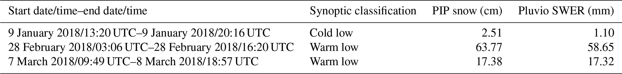

Figure 1Time–height plots of vertical profiles of ZH (first row), ZDR (second row), Kdp (third row), ρhv (fourth row), and DWR (fifth row) for the 9 January 2018 (left column), 28 February 2018 (middle column), and 7–8 March 2018 (right column) cases.
The D3R Zdr and ϕdp were calibrated on an event basis, and the absolution calibration of Ku and Ka Z was established in the early period of the deployment (Chandrasekar et al., 2018). Notwithstanding these calibration efforts, in order for the retrieval algorithm to perform optimally, we examined the data for self-consistency of Zdr and the dual-wavelength ratio (DWR), defined as ZKu−ZKa. The expectation is that, at near-zenith angles, Zdr should be close to zero, and, in the limit of small particles, the DWR should equal the difference in attenuation, which should be small, but positive, depending on the path-integrated attenuation from water vapor, cloud liquid water, and hydrometeors.
We examined time series of the PDFs of these quantities for the events listed in Table 1. In Fig. 2, the top two rows show the time series of the PDF of Ku and Ka Zdr at elevation angles and altitudes above 1.5 km m.s.l. There is clearly some non-stationary behavior in these PDFs, so we applied additional calibration offsets (independently at each frequency) to the Zdr for each RHI such that the average Zdr at elevation angles is equal to zero. The time series of the calibrated Ku and Ka Zdr are shown in the third and fourth rows of Fig. 2. In addition to the modification to Zdr, we also noticed some unusual behavior in the small-particle DWR PDF (fifth row of Fig. 2) during the 28 February case. When ZKu<10 dBZ, Skofronick-Jackson et al. (2019) found that Ku–Ka DWR is typically close to zero, but during this case, there is large increase in the DWR, peaking around 06:00 UTC, that is difficult to explain entirely by particle size or attenuation. Accumulation of wet snow on the radome is a possible explanation for this behavior (Venkatachalam Chandrasekhar, personal communication, 2020), but for this study we have chosen to avoid correcting the DWR because it is difficult to have a continuous independent estimate of the Ku–Ka relative calibration from a ground radar.
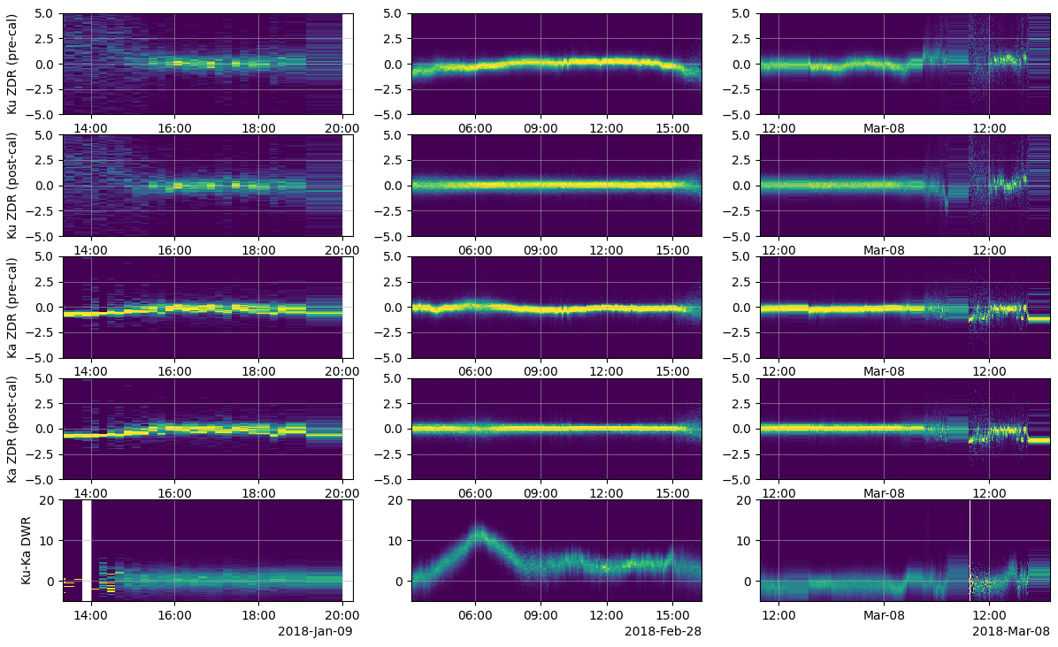
Figure 2Time-series histograms of near-zenith Ku Zdr before (top row) and after (second row) offsets were applied. Similar histograms are presented for Ka-band data in rows three and four. The fifth row displays the time-series histogram of the Ku–Ka DWR where Ku reflectivity is less than 10 dBZ within 10 km of the radar. Colors are indicative of relative occurrence, normalized at each time step.
2.2 PIP
The primary source of validation for the microphysical retrievals in this study is PIP (Pettersen et al., 2020), which takes measurements that can be used to derive quantities including snowfall rate and effective density. The PIP is a video disdrometer made up of a single high-speed camera, continuously recording at 380 frames per second, and a halogen lamp, which is used to backlight the precipitation particles. The camera and lamp are separated by 2 m and the focal plane is located 1.33 m from the camera lens and uses an open sampling volume (i.e., the sampling volume is not enclosed within a box). The images produced are 640×480 pixels with a resolution of 0.1 mm×0.1 mm. The field of view (FOV), including the edge effects, is then 64−Deq mm mm, where Deq is the equivalent diameter in millimeters. The depth of field (DOF) also varies with particle size and is expressed as (in mm). The sampling volume is a multiplication of the FOV, DOF, and the number of frames over a given time period. Considering 100 particles with uniform size of Deq=1 mm, the sampling volume is 790 m3 for a 1 min observation period. As PIP only uses a single camera, the precipitation particle images are of a projected view of the particle and do not contain any information on the particle dimension along the viewing direction.
PIP determines the characteristics of the precipitation particles using an algorithm written using the National Instruments IMage AQuisition (IMAQ) software package. This algorithm determines the shape of the precipitation particle (i.e., the long and the short dimensions) by fitting an ellipse to the PIP-imaged particle. The IMAQ software package defines the fitted ellipse as the ellipse having both the same area and the same perimeter as the PIP-imaged particle. During our preliminary analysis of the data, we found that the IMAQ-fitted ellipses tended to overestimate the long dimension of the particle and underestimate the short dimension, resulting in an underestimate of the aspect ratio. As such, we have reprocessed the PIP data using an alternative, custom-built ellipse-fitting strategy (Helms et al., 2022). This strategy uses the method implemented in the fit_ellipse program in the Coyote Interactive Data Language (IDL) library (http://www.idlcoyote.com/, last access: 25 February 2022) to perform the actual fit. The fitting is performed on images of particles taken from videos that PIP records for troubleshooting purposes. These videos contain the first 2000 frames that contain precipitation particles within each 10 min period. For periods with fewer than 2000 frames containing precipitation particles, the videos will be shorter than 2000 frames.
The PIP-determined orientation angle is defined as the counterclockwise angle from the positive horizontal axis, where positive is to the right, to the longest dimension of the particle. This results in orientation angles ranging from 0 to 180∘. In order to combine the ellipse aspect ratio (minor axis length divided by major axis length) and orientation angle information, we have used the natural logarithm of the aspect ratio of the bounding box of the particle. The bounding box is defined as the smallest rectangle that is able to contain the particle and whose edges are either horizontally or vertically oriented.
2.3 Soundings
Radiosonde launches were performed every 3 h during precipitation events from the DGW Regional Weather Office, supplementing the normal 12-hourly observations, and used Meteomodem M10 radiosondes (Meteomodem, 2021). The profiles of temperature and humidity from the nearest-in-time radiosonde were used as input to the D3R algorithm to calculate attenuation from atmospheric gases. These profiles are also used to qualitatively evaluate the retrieval output with respect to locations of well-known thermodynamic importance (e.g., the −15 ∘C dendritic growth maximum and layers that are supersaturated with respect to ice).
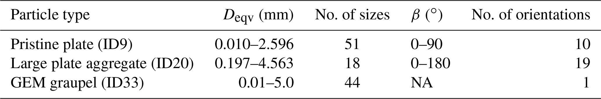
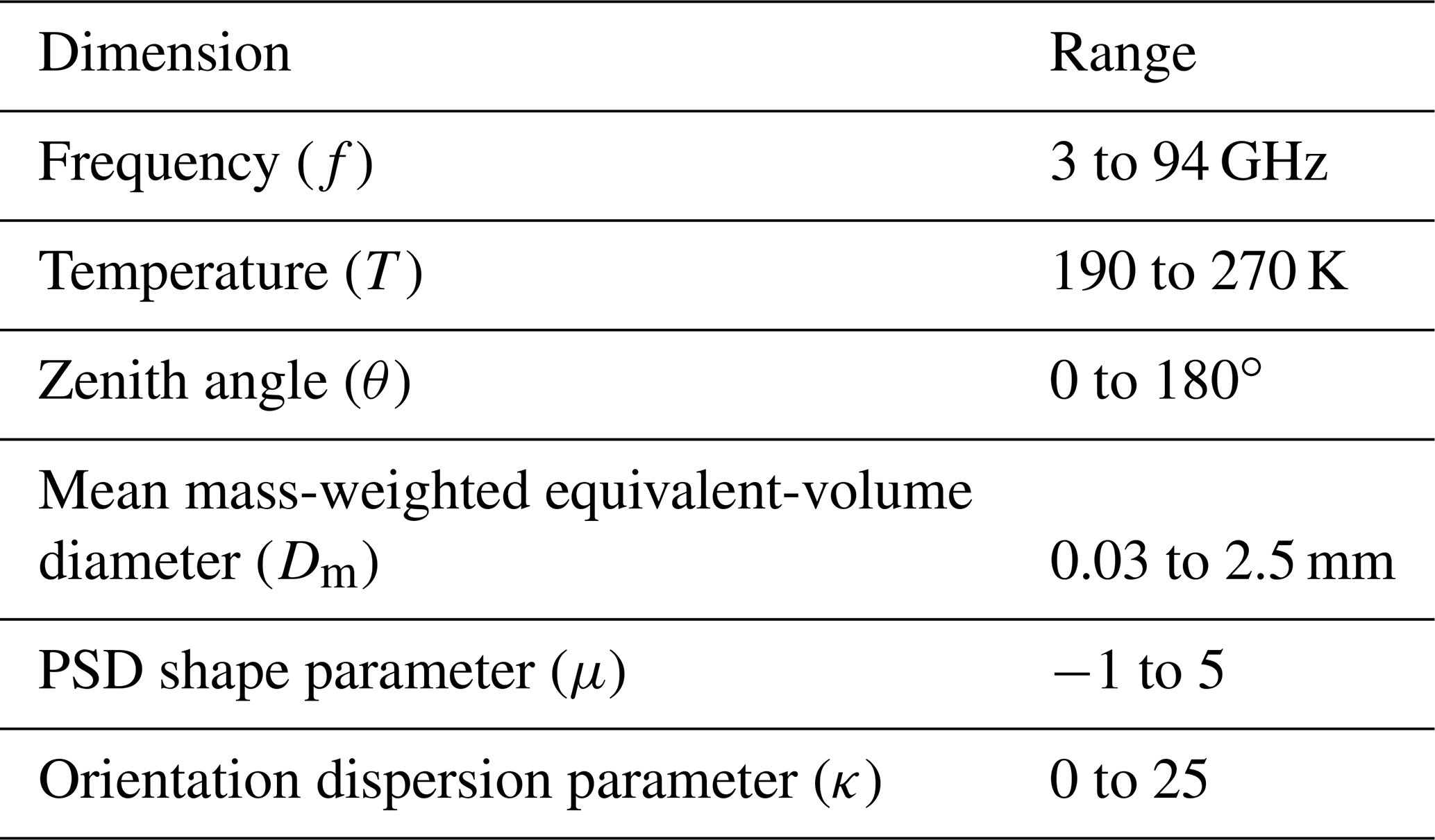
Gaining useful information from polarimetric radar measurements requires scattering properties of hydrometeors with preferred mean orientations. We incorporate such scattering properties into the retrieval algorithm described herein, by way of lookup tables (LUTs) that are derived by integrating these scattering properties over a prescribed PSD. Specifically, we use scattering properties for a pristine plate, an aggregate of plates, and graupel (all at a wide range of sizes) from the Atmospheric Radiative Transfer Simulator (ARTS; Eriksson et al., 2018; Brath et al., 2020; Ekelund et al., 2020) database. Scattering properties for each of these particles are available for a discrete set of frequencies (for this study, we use the calculations at 13.4 and 35.6 GHz), temperatures (190, 230, and 270 K), incident angles of the transmitted radiation, scattering angles of the scattered radiation, and, except for graupel (which is assumed to have total random orientation) zenith-relative orientation angles (we refer to this angle hereafter as β). Table 2 lists values of these properties that correspond to the scattering calculations.
Table 2Properties of the ARTS scattering database calculations used herein.
NA: not available.
The ARTS database aims to provide scattering properties for a set of particles over a large range of frequencies so that applications using both active and passive remote sensing measurements are consistent. The derivation of polarimetric radar variables from this database is described in Appendix A. For each particle type listed in Table 2, these variables are integrated over a PSD using a modified gamma form (e.g., Petty and Huang, 2011):
where D is the diameter of an equivalent-volume solid ice sphere in mm, Dm is the mass-weighted mean equivalent-volume diameter, and μ is the shape parameter. While this definition of D (and Dm) complicates the comparison to in situ measurements (where maximum dimension is typically used to describe size), it is directly related to particle mass, and, in the Rayleigh limit, radar reflectivity. To reduce the dimensionality of the LUTs while preserving the variables that control the shape of the PSD, only Dm and μ are varied in the construction of the LUT, and N0(Dm,μ) is a normalized concentration factor such that the ice water content of all PSDs stored in the LUT is 1 g m−3:
where ρi is the density of solid ice (0.917 g cm−3). The distribution is later scaled by a retrieved concentration factor to match the observed reflectivity. For the particle types with preferred orientation, these PSDs are further integrated over the range of β angles to account for the orientation distribution. We choose the von Mises distribution to represent the PDF of beta angles (Table 2). The von Mises distribution is a continuous function that represents the dispersion of variables in circular coordinates, and has been used to represent hydrometeor orientation retrieved from polarimetric radar (Bringi and Chandrasekar, 2001; Melnikov and Straka, 2013). For a zero-mean canting angle, this distribution simplifies to
where κ is a dispersion parameter and G(κ) is a normalization factor such that the sum of probabilities is equal to 1. When κ=0, the distribution is uniform; as κ increases, the distribution becomes narrower and can be approximated by a normal distribution with standard deviation . In the construction of the LUTs, we make the simplifying assumption that κ is independent of particle size. While this is almost certainly an oversimplification (observations and Reynolds number analysis suggest that smaller particles of a given aspect ratio should have more randomly distributed canting angles; Klett, 1995), in the retrieval, this is dealt with by allowing the combination of pristine and aggregate PSDs of different κ values, as will be further described in Sect. 4.
Table 3Dimensions of the lookup tables derived from the particle types selected from the ARTS single-scattering database.
The LUTs are constructed for each particle species. The LUT dimensions and ranges of the LUT indices are given in Table 3. The variables stored within the LUTs encompass three categories: radar variables, physical variables, and simulated PIP measurements. The radar variables are the single-particle scattering properties necessary to construct the polarimetric radar measurements: the reflectivity factor Z at both horizontal and vertical polarizations, the extinction coefficient k at both polarizations, the specific differential phase Kdp, and the real and imaginary parts of the co-polar conjugate product of scattering amplitudes (). The formulas used to forward model the radar measurements from these quantities are given in Appendix B.
In addition to the radar variables, we simulate several variables (denoted with subscript P) that represent PIP-measured quantities. Because the PIP measures 2-D projections of 3-D particles, assumptions must be made to convert the PIP measurements to physical variables. While several formulas have been proposed to achieve this purpose (e.g., Jiang et al., 2017), we opted instead to use 2-D projections of particles derived from the shapefiles used in the ARTS database to simulate the PIP measurements over the range of Dm, μ, and κ in the LUTs, as this process is less ambiguous than the alternative of attempting to derive the 3-D properties from the 2-D PIP measurements. Moreover, this process ensures an internally consistent comparison of the radar retrieval output with PIP measurements. Most of these quantities depend in some way on the equivalent diameter Deq measured by the PIP. The simulated PIP measurements include the snowfall water equivalent rate (S), volumetric snowfall rate (SV), effective density (ρP), normalized intercept , area-weighted mean particle volume diameter DP, mean box aspect ratio (), and mean ellipse aspect ratio (). The final two quantities are weighted by the projected area. The snowfall water equivalent rate is calculated as
where m(D) is the mass of the particle in grams, Vt(D,β) is the terminal velocity in m s−1, and S is in units of mm h−1. The terminal velocity is calculated following the process given in Heymsfield and Westbrook (2010), where the area ratio is simulated from the ARTS shapefiles (and thus depends on both D and β), and using values for the density and viscosity of air typical at the MHS location during ICE-POP 2018 snow events (−5 ∘C, 90 %RH, 925 hPa). The volumetric snowfall rate is calculated using the same terminal velocity but, instead of mass, using the volume of the particle derived from the PIP-measured diameter:
The PIP-derived density (ρP) is defined as the ratio of the liquid-equivalent snow rate to the volumetric snowfall rate multiplied by the density of liquid water ρw (Tiira et al., 2016):
The normalized intercept is adapted from the definition given for in Field et al. (2005):
where dmax2D(D,β) is the average 2-D projected maximum particle dimension. This parameter is useful for providing temperature-dependent constraints on the PSD as will be shown in Sect. 4.
DP is the ratio of the fourth to third moments of the PSD in terms of Deq:
In order to evaluate the capability of the D3R polarimetric measurements to retrieve a bulk measurement of the aspect ratio, we defined the area-weighted mean ellipse aspect ratio ():
where is the ratio of the short to long axis of the ellipse fitted to the simulated PIP image. In order to compare our retrievals to a variable that is influenced by the canting angle distribution parameter κ, we defined the area-weighted mean box aspect ratio ():
where is the ratio of the vertical to horizontal dimensions of the bounding box of the simulated PIP image.
While it is not feasible to illustrate every dimension of the LUTs, a few examples are provided to preview the expected sensitivity of the D3R measurements to microphysical parameters. In Fig. 3, the Ku–Ka dual-wavelength ratio is plotted as a function of both the volume-equivalent Dm and PIP-measured DP for each of the three species. The DWR is nearly identical for the pristine plates and plate aggregates at Dm<1 mm and DP<3 mm but reaches an upper limit of about 5 dBZ for the single plates while increasing to nearly 10 dBZ for the aggregates. Large Ku–Ka DWRs, sometimes exceeding 10 dBZ, have been observed coincident with large aggregates (20 mm projected diameter) in dendritic growth regimes during OLYMPEX (Chase et al., 2018), so it is important that the LUTs capture this DWR range. The DWR of graupel is lower than the unrimed plates and aggregates for a given volume-equivalent size but is similar or greater when viewed with respect to PIP-measured size based on the projected area. This suggests that DWR alone is not sufficient to determine the PSD mean particle size and density. Such information can be provided by the polarimetric measurements. For this study, we assume graupel to be randomly oriented and thus have zero contribution to Zdr and Kdp, which is a reasonable assumption for dry graupel (Kumjian, 2013). Meanwhile, the contributions to Zdr and Kdp from plates and aggregates primarily depend on Dm and κ (Fig. 4). As expected, both Zdr and Kdp increase with κ as the orientation distribution becomes less dispersive. The Zdr rapidly decreases with aggregate size, as does Kdp (though less rapidly). Meanwhile, the Zdr of the individual plates does not depend on Dm, since these plates have a fixed aspect ratio at sizes larger than about 0.2 mm (Brath et al., 2020). The Kdp of the individual plates also does not depend much on size, although some resonance effects lead to a small decrease in Kdp at larger size. From Figs. 3 and 4, it is clear that there is complementary information in the dual-frequency and polarimetric variables to discern particle size and species, which will be demonstrated in the next section.

Figure 3Ku–Ka dual-wavelength ratio for the three ice species listed in Table 2 as a function of the melted (volume equivalent) Dm (a) and DP (b). The families of curves represent different values for the shape parameter μ ranging from −1 to 5, with lighter shades indicating higher values and less dispersion of the PSD. The different ranges of DP are a consequence of the different size–density relationships for each species.
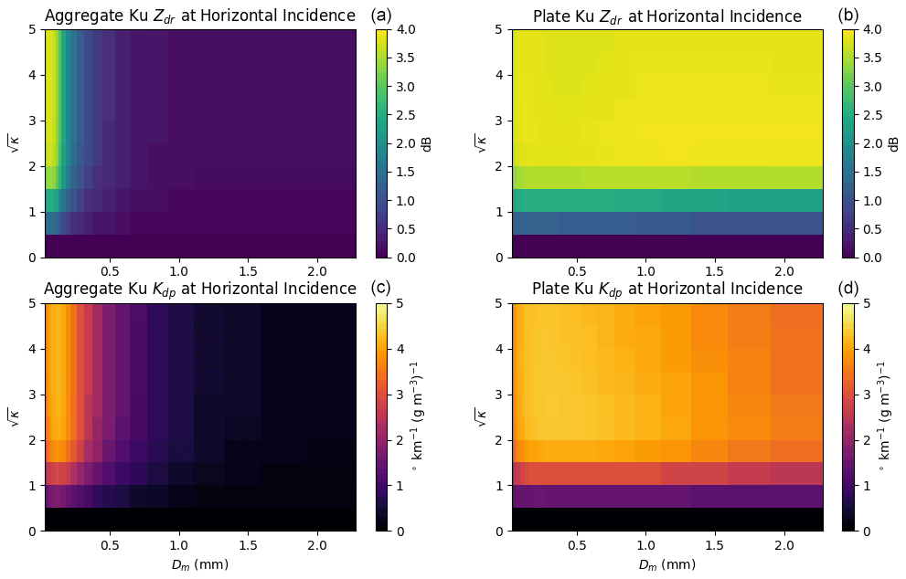
Figure 4Polarimetric variables Zdr (a, b) and Kdp (c, d) as a function of mean particle size Dm and orientation distribution parameter κ. Panels (a, c) represent aggregates, and (b, d) individual plates. All values are for horizontal incidence at the Ku band at 270 K.
Optimal estimation (OE; Rodgers, 2000) is a form of Bayesian inversion that assumes Gaussian error statistics and accommodates moderately nonlinear forward models. OE has been used for single-frequency (L'Ecuyer and Stephens, 2002; Munchak and Kummerow, 2011) and multi-frequency (Grecu et al., 2011; Mason et al., 2018) radar precipitation retrievals. It is applied here to the multi-frequency, polarimetric observations provided by the D3R. In this section, the OE components (state vector, observation vector, and covariance matrices) are defined and the approach is illustrated with an example retrieval along a single radar ray.
4.1 Optimal estimation setup
The cost function that is minimized by optimal estimation is
where Yobs is the observation vector and Ysim(X) its forward-modeled counterpart, Sy is the measurement and forward model error covariance matrix, X is the state vector and Xa its prior, and Sa is the state covariance matrix. For the D3R retrieval of snow microphysical properties, we define Yobs to contain one or more of the following series of dual-frequency or dual-polarization observations at each range gate along a radial:
where each type of observation is filtered for ground clutter and only considered if the signal-to-noise ratio exceeds 1. Thus, the number of observations of each type may differ. Note that ϕdp instead of Kdp was chosen because ϕdp is the more direct measurement, and additional assumptions (with potentially non-Gaussian errors) are required to derive Kdp from noisy ϕdp measurements.
The state vector consists of quantities that describe the PSD, relative contribution of each species, as well as other quantities known to affect the Ku- and Ka-band polarimetric radar measurements:
where each quantity is defined at nodes (indicated by the superscript in Eq. 13) which may be arbitrarily placed (for this study, nodes are spaced 600 m horizontally and 250 m vertically). Each of these quantities, their priors, and ranges are defined in Table 5. Following Grecu et al. (2011), the measured Ku-band Zhh (which is not in Yobs) is used as direct input to the forward model, and from these measurements and the quantities in the state vector X, the measurements in Yobs are simulated. A detailed description of this forward model is provided in Appendix B.
Field et al. (2005)Table 5Names, definitions, a priori value, standard deviation, and allowed ranges of quantities in the state vector (Eq. 13). Note that some quantities are retrieved in logarithmic space to accommodate lognormal distributions and/or to linearize the forward model. SD: standard deviation.
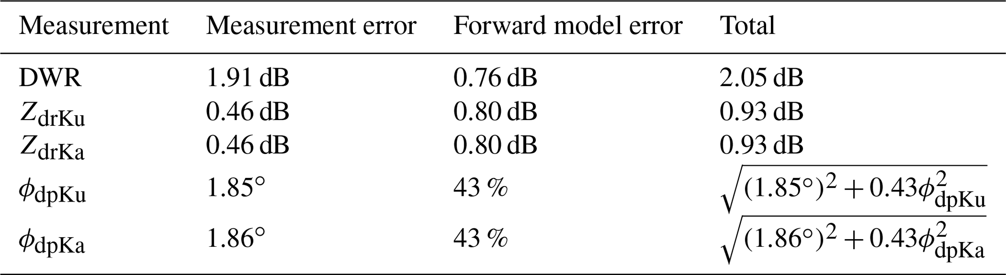
The observation error covariance matrix Sy must accurately describe the error characteristics of the measurements and forward model. Values that are unrealistically low can lead to overfitting, whereas overly conservative (large) error estimates can lead to underutilization of the information contained within the measurements. In this study, we consider the diagonal elements of Sy to be the sum of the measurement error and forward model error components, which are given in Table 6 for each measurement in Sy. The measurement errors are obtained from the gate-to-gate variance over many homogeneous scenes at low (<10∘) elevation angles, where the assumption is that the true change in the measured quantity is small compared to the measurement noise. The measurement error is assumed to be uncorrelated in space and between variables. The forward model error is quantified by assessing the variance in the measurements for alternate aggregate particles of the same size as the ARTS aggregates. These alternate models include dendrites and columns, with different assumptions about the aggregation process (Schrom et al., 2021). Although these forward model errors are correlated between variables, analysis of the covariance matrices showed the correlation between DWR and Zdr error to be insignificant. While Zdr−Kdp error correlation is larger, the ϕdp error is dominated by upstream propagation error which is assumed to be uncorrelated to the Zdr forward model error at a given range gate. Therefore, for this study, the off-diagonal elements of Sy are set to zero, although this is a choice that could be refined in future implementations of the retrieval.
Table 6Measurement and forward model components of the error covariance matrix Sy for each measurement, expressed as standard deviations.
4.2 Example ray
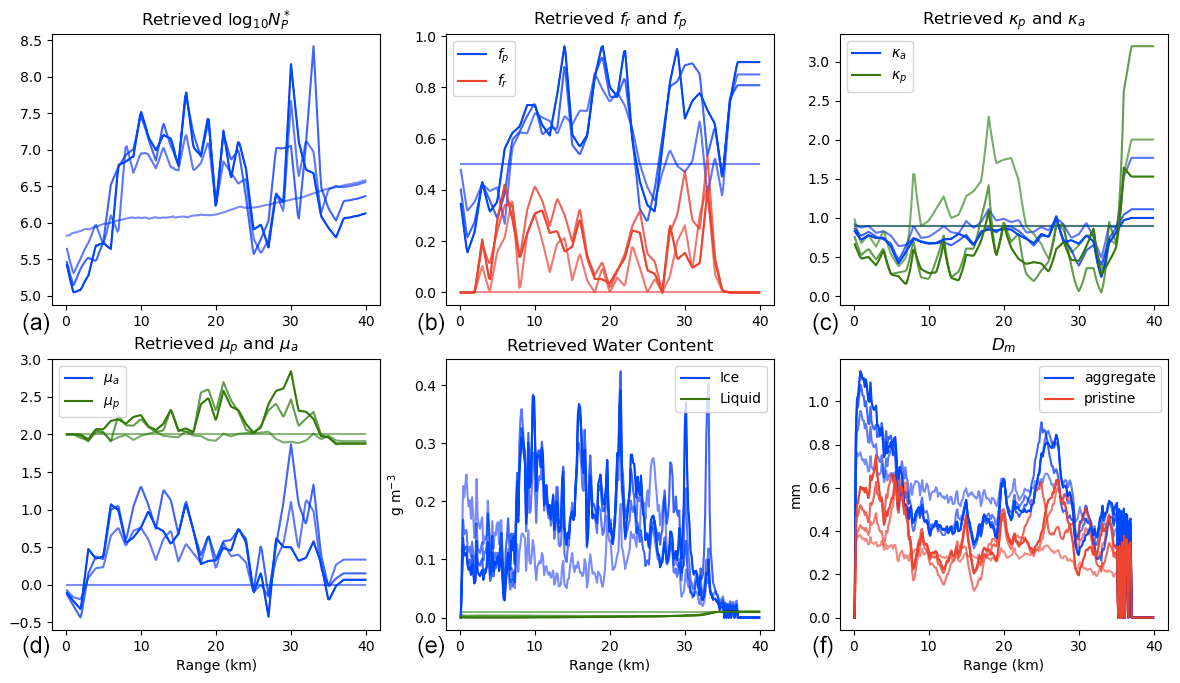
The optimal estimation process along a ray of radar data is illustrated in Fig. 5, which shows the observed (Yobs) and simulated (Ysim) measurements, and Fig. 6, which shows the various retrieval parameters in X as well as derived quantities of ice water content and Dm for each iteration until convergence. This ray is characterized by DWR peaks at 0–5 and 23–28 km, which reach 6 dB, dropping to 1–3 dB elsewhere. The Zdr has several peaks, the most significant of which reach over 2 dB at 20 and 30 km range, bracketing the DWR peak. The ϕdp increases most rapidly in the 10–20 km range with smaller rates of increase elsewhere, reaching 15∘ at the Ku band and 50∘ at the Ka band. The initial profiles of the retrieval parameters , fr, fp, κp, κa, μp, μa, and the derived ice and cloud liquid water content and Dm of the aggregate and pristine PSDs are shown in the lightest shaded lines in Fig. 6. The iterative adjustments guided by the Jacobian matrix respond to the initial differences between Yobs and Ysim:
-
decreases slightly near the DWR peaks and increases elsewhere.
-
fp decreases below 50 % in the DWR peak region but increases above 60 % in the 10–20 km range and again near 30 km, corresponding to the Zdr peaks and steepest increase in ϕdp.
-
fr is generally below 40 %, with minima near the Zdr peaks.
-
κp is generally lower than κa but exhibits peaks corresponding to the Zdr peaks, whereas κa does not vary as much with range.
-
μa and μp increase slightly from their initial values in most regions, although μa dips below zero near the DWR peaks (lower μ corresponds to a longer tail of the PSD at large sizes and can result in higher DWRs, all else being equal).
-
No significant cloud liquid water is detected or needed to explain the DWR observations. In fact, the near-zero DWR at the far ranges implies that there is little differential attenuation, and the observed near-field DWR can be attributed to particle size effects.
-
Dm of the pristine population (controlled by the retrieval parameter Dp) generally increases as a proportion of the Dm of the aggregates in order to balance pristine particle contributions to Zdr and ϕdp.

Figure 5D3R observations of reflectivity (a) and DWR (d), Zdr (b, e), and ϕdp (c, f) along the 231∘ azimuth, 6∘ elevation radial at 02:17 UTC on 8 March 2018. For the DWR, Zdr, and ϕdp, the D3R observations are indicated by the solid black lines and the simulated measurements for each iteration are shown in progressively more opaque blue lines, with the final iteration plotted in red.
The most significant impact of these parameter changes is to increase Dm and reduce ice water content in the DWR peak regions, with the opposite changes elsewhere. The final retrieved state is in good agreement with the Zdr and ϕdp observations at both frequencies. There is a residual high bias in the DWR, especially at the range beyond 30 km. Examining the DWR histogram for this case in Fig. 2 reveals a mean near or below zero, which may indicate a low bias in the relative calibration of the Ku to Ka reflectivity, and possible high bias in the ice water content retrieval.
As a consistency check, we show that the retrieval algorithm effectively reproduces the spatial distribution of the radar variables for an RHI (Fig. 7). The retrieval that uses only the DWR as input is able to reproduce the reflectivity and dual-wavelength ratio measurements but overestimates the Φdp at both wavelengths and poorly represents the spatial structure of the ZDR. In contrast, the retrieval using only the Ku-band polarimetric measurements produces simulated Φdp and ZDR that correspond well to the measurements but dual-wavelength ratio simulations that fail to capture the observed dual-wavelength ratio structure in the RHI. The simulated radar variables associated with the retrieval that incorporates all of the radar observations shows the best consistency with the observations, suggesting that the polarimetric and DWR measurements contain independent and complementary information.
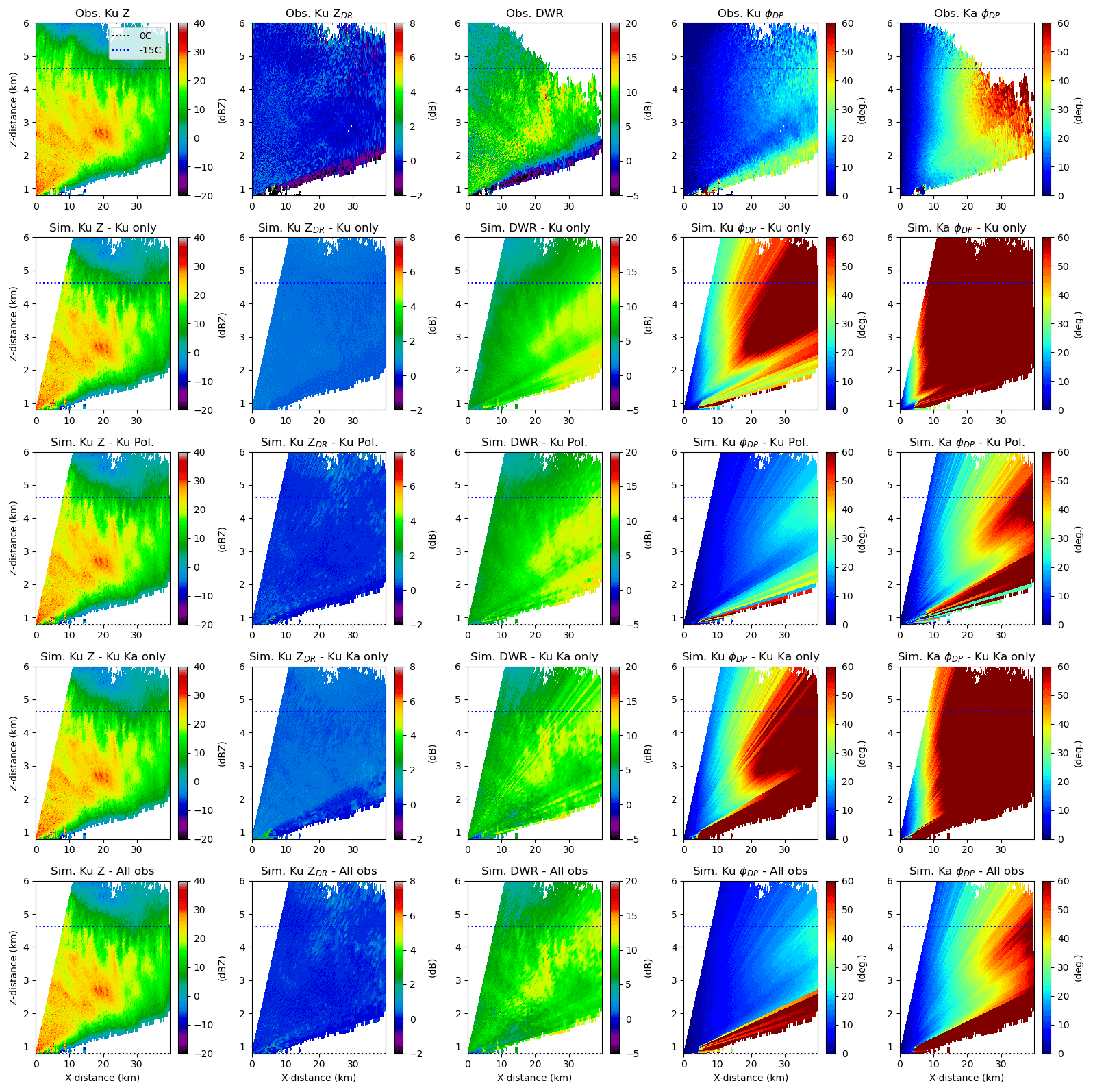
Figure 7Observed and simulated ZH (first column), Ku-band ZDR (second column), DWR (third column), Ku-band Φdp (fourth column), and Ka-band Φdp (fifth column). The observed radar variables are shown on the first row, the simulated radar variables from the Ku-band reflectivity retrieval are shown in the second row, the simulated radar variables from the Ku-band polarimetric retrieval are shown in the third row, the simulated radar variables from the Ku-band and Ka-band reflectivity retrieval are shown in the fourth row, and the simulated radar variables from the full-observation retrieval are shown in the fifth row. The observations are from an RHI taken at 13:00 UTC on 28 February at an azimuth angle of 231∘.
4.3 Information content analysis
Some further insight into the adjustments made to the parameters can be gained by examining the Jacobian matrix K of partial derivatives of each element of Ysim with respect to each element of X.
While the Jacobian is state dependent, the sign and relative magnitude of each element from the example ray shown in the previous section are illustrative of the general sensitivity of the forward model to the retrieval parameters. The Jacobian matrix is composed of blocks that are either diagonal or triangular, depending on whether the parameter has a significant downrange propagation effect on an observation. The effect of modifying the parameters in X can be explained by considering the change to the PSD at a fixed Ku-band reflectivity:
-
Increasing results in a smaller mean particle size and higher ice water content. This decreases the DWR and increases ϕdp downrange, while the effect on Zdr is relatively small and state dependent.
-
Increasing fp increases Zdr and ϕdp downrange as a result of the increasing contribution of the pristine particles to the PSD, with little effect on DWR.
-
Increasing Dp also increases Zdr (and decreases DWR) as the pristine particles become larger and contributes more to reflectivity but decreases ϕdp downrange as the ice water content is reduced.
-
Increasing κa and κp increases the Zdr and downrange ϕdp, with the κp having a much larger magnitude effect.
-
Increasing μa reduces the DWR as the large-particle tail of the PSD is truncated. There is almost no impact of changing μp on the simulated observations.
-
Increasing cloud liquid results in an increase in the downrange DWR due to increased differential attenuation but has no impact on the polarimetric measurements.
-
Increasing fr reduces the DWR and all of the polarimetric measurements, as the rimed particles are assumed to have random orientation.
It is noteworthy that the sign of the observation response to perturbations varies in different ways for the different parameters in X. This is an indication that this optimal estimation retrieval, as we have formulated it, is well determined and is also a requirement for reducing ambiguity, or cross talk, in the retrieved state. The information content and cross talk among parameters can also be evaluated by examining the averaging kernel matrix of the retrieved state. The averaging kernel provides a measure of influence of the observations on the retrieved state and is defined as
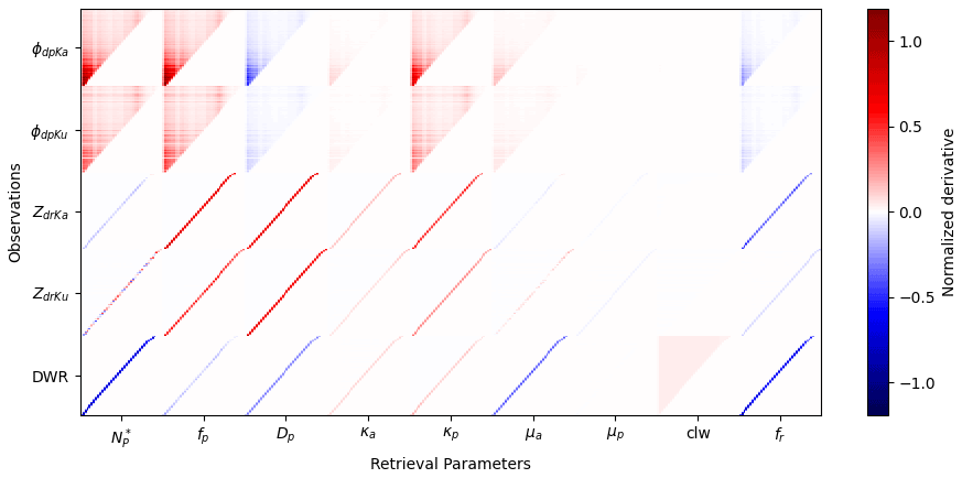
Figure 8Jacobian matrix of partial derivatives of the simulated D3R measurements to the retrieval parameters. The partial derivatives have been normalized element wise by the square root corresponding diagonal element of Sy – i.e., the expected standard deviation of that measurement's error.
Values close to 1 indicate strong influence of measurements, and values close to 0 indicate that the retrieval is heavily influenced by the prior. In Fig. 9, the median, 10 %, and 90 % quantiles of the averaging kernel are plotted. These statistics were derived from many retrieved states spanning the cases we examined in Table 1. The parameter with the highest information content is the normalized intercept (), which both the DWR and ϕdp are highly sensitive to (Fig. 8). The two parameters that describe the pristine component of the PSD (fp and Dp) also have a similar median and 90 % quantile values to , due to their sensitivity to the polarimetric parameters, but a lower 10 % quantile, likely originating from situation where the fr is high and there is little sensitivity of the polarimetric variables to fp and Dp. Similarly, κp has a large range between the 10 % and 90 % quantiles, indicating that the information content of this parameter is state dependent, and high values of fp and Dp are required to maximize the sensitivity of the polarimetric observations to this variable. Another parameter with a wide range of averaging kernel diagonal values is fr, which requires low fp and Dp values for it to be the primary driver of the polarimetric variables. Some of this state dependence of the information content is also reflected in the off-diagonal values, which indicate significant cross talk, i.e., a strong correlation in the posterior state vector, between the following groups of variables: , μa, fr; and fp, Dp, κp. These groups have similar Jacobians making it difficult to determine them independently. Finally, it is notable that a few of the variables (κa, μp, and cloud liquid) have very low averaging kernel values, indicating that the observations are not particularly sensitive to them. This is not surprising, since the aggregates do not show much Zdr or Kdp sensitivity to κ except at the smallest sizes (Fig. 4), and the shape parameter (μ) of the pristine PSD is not going to influence the reflectivity observations (DWR and Zdr) because the shape of the large-particle tail is only important to these observations if Dp is close to its upper limit of 1. The sensitivity of Zdr and Kdp to κ does depend on the aggregate shapes. The ARTS large plate aggregate used herein may not represent cases of more horizontally exaggerated aggregates where the assumed orientation will have a larger impact on the simulated polarimetric variables. The low averaging kernel values for cloud liquid are reflective of the result that it was rarely retrieved in significant quantities, and since it is treated logarithmically, only large values will induce large changes to the DWR. However, there were several RHI scans, particularly on 28 February, where some cloud liquid was necessary to explain high DWR values that could not be achieved by differential scattering alone.

Figure 9Quantiles of the averaging kernel matrix diagonal elements and off-diagonal elements representing different parameters at the same range gate.
The primary tool used for validation of the D3R retrievals is the PIP located at the MHS location. The D3R retrievals were matched to the PIP by averaging the retrieved quantities in a 600 m wide by 500 m tall box centered above MHS. The lower altitude limit of this box was placed 250 m above the surface to avoid ground clutter contamination along the radials used for averaging. To evaluate the impact of the dual-frequency and dual-polarization measurements, four retrieval experiments were conducted:
-
Ku-only: a single-frequency retrieval, equivalent to prescribing a temperature-dependent Z−S relationship;
-
DWR-only: a dual-frequency retrieval without polarimetric information; similar information content to the GPM dual-frequency precipitation radar (DPR);
-
Ku-pol: a single-frequency polarimetric retrieval using Zdr and ϕdp at the Ku band only;
-
All-obs: a dual-frequency polarimetric retrieval using DWR and the Zdr and ϕdp at both frequencies.
To assess the quality of the PIP–D3R matchups, the Ku-band reflectivity was calculated directly from the PIP-derived PSDs using Mie theory (spherical particles) with the PIP-derived particle densities (Tokay et al., 2022). Although there will be some departures from Mie theory for non-spherical particles, at the Ku band these are relatively small (Kuo et al., 2016). The larger contribution to error is the various assumptions required to derive particle density from the PIP size and fall speed (Tokay et al., 2022). Using an ensemble approach to these assumptions, a range of reflectivities was obtained and compared to the D3R-observed reflectivity in the averaging box (top row of Fig. 10).
Some different tendencies are noted for each event. The 9 January case had a consistently higher PIP-derived reflectivity than the D3R measurement, especially during the middle hours of the event. This was a low-echo-top cold low case, and D3R-derived time–height profiles (Fig. 1) indicate significant echo growth (perhaps due to aggregation) at low levels, which may have continued in the clutter region. The 28 February case exhibits a similar bias between the PIP-derived and D3R-measured reflectivity at the Ku band in the first 6 h, after which the D3R reflectivity comes within the lower range of PIP estimates. This was a deeper, warm low case, and the D3R profiles do not indicate any substantial reflectivity increase towards the surface. Instead, it is suspected that excess attenuation from wet snow (the wet bulb temperature was above 0 ∘C until 04:00 UTC and the air temperature was above 0 ∘C until 08:00 UTC) accumulated on the radome is responsible for these differences (note also the sharp increase in DWR during the same time period attributed to this factor in Sect. 2). The 7–8 March case exhibited the best agreement between PIP-derived and D3R-measured reflectivity throughout the event. This was also a warm low case with deep echo tops but colder wet bulb temperatures (between −4 and −2 ∘C during the event).
The validation statistics presented in this section are derived from matchups of the D3R-derived and PIP-measured quantities listed in Table 4. Because the PIP measurements are taken every minute, whereas the D3R RHI scans were conducted every 5–6 min, an optimal lag was found by maximizing the correlation between the lagged D3R-measured and PIP-derived Ku-band reflectivity time series. This lag time was between 2–7 min, depending on the event, which is consistent with a fall speed slightly greater than 1 m s−1 to cover the distance from the center of the averaging box to the surface. Only retrievals where the D3R-measured Ku band reflectivity was within the range of PIP estimates were considered in the calculation of statistics to ensure that the PIP measurements are reasonably representative of the D3R observations.

Figure 10Time series of D3R-observed and PIP-simulated Ku-band reflectivity (top row), D3R-observed DWR (second row), D3R-observed Zdr (third row), and D3R-derived Kdp for each event. The PIP simulations used Mie calculations for spherical particles with the PIP-derived effective density. Because these calculations involve a variety of assumptions to derive density from particle shape and fall speed (Tokay et al., 2022), a range between the minimum and maximum from these calculations is shaded around the mean PIP-derived value.
5.1 Snowfall rate and water equivalent
The time series of snow water equivalent rate (S) for each event are shown in Fig. 11. The D3R substantially underestimates snowfall throughout the 9 January and 28 February events, which is not surprising since the PIP-derived reflectivity significantly exceeds the D3R measurement for reasons discussed previously in this section. It is worth noting, however, that the DWR-only and All-obs retrievals are in good agreement with the Pluvio-measured S accumulation on 9 January, which would be consistent with aggregation processes in the lowest levels that increase reflectivity but do not increase S. The 7–8 March event shows better agreement with the PIP measurements. In this case, which had the best reflectivity match, the DWR-only retrieval overestimates S, whereas the Ku-only and Ku-pol retrievals underestimate S relative to the PIP. The retrieval using all of the observations is the closest match and the accumulated S falls within the range of PIP estimates for most of the event. We note from the DWR time series for this event in Fig. 10 that the DWR is just above 0 dB for much of this event which implies a smaller mean particle size and higher S for a given reflectivity. Meanwhile, the Ku-pol retrieval gives a slight reduction in S from the Ku-only retrieval, which is already biased low for this event. Compared to the Pluvio, the All-obs retrieval is biased high; however, after correcting the Pluvio data for wind (Milewska et al., 2019), this retrieval is in better agreement. However, these same wind corrections bias the 9 January event higher than the retrievals and in better agreement with the PIP.
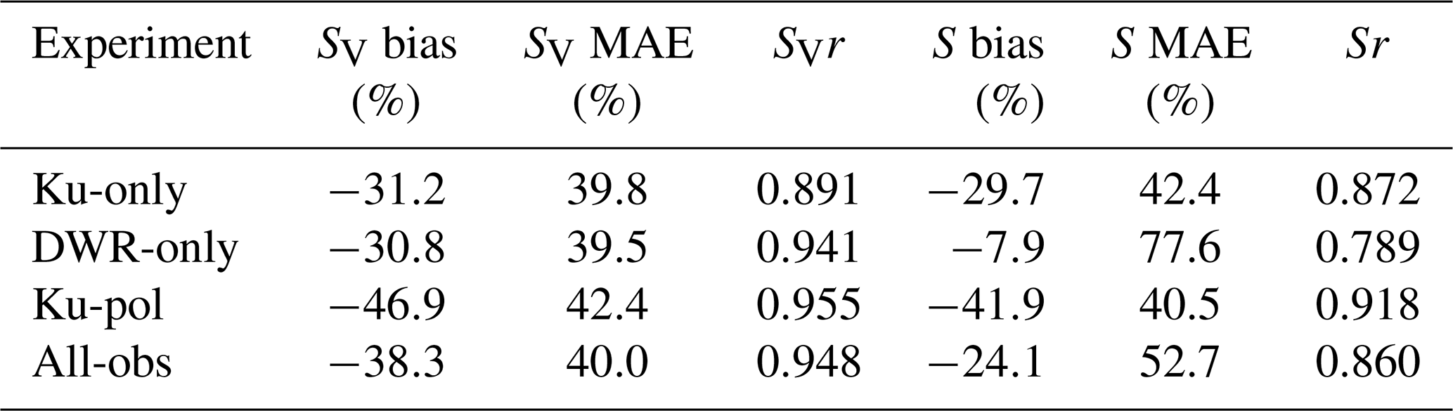
Error statistics for volumetric snowfall rate (SV) and S from all events, filtered for times when the D3R-measured reflectivity was within the PIP-estimated range, are presented in Table 7. The bias is the overall fraction difference between the accumulated PIP- and D3R-derived amounts. All methods underestimate the amounts, with the DWR-only method providing the closest match for both SV and S. However, this appears to be the result of compensating biases on the 28 February and 7–8 March events, and the mean absolute error (MAE) is highest for this method. The Ku-pol method provides the best correlation for SV and S even though it has the largest magnitude bias of all the experiments. The high correlation coefficients, particularly for the multi-parameter methods, are indicative of a response of the radar measurements to the microphysical properties that determine snowfall rate, but the large biases indicate either a calibration bias in the observations, biased forward model (i.e., unrepresentative scattering properties), or both.
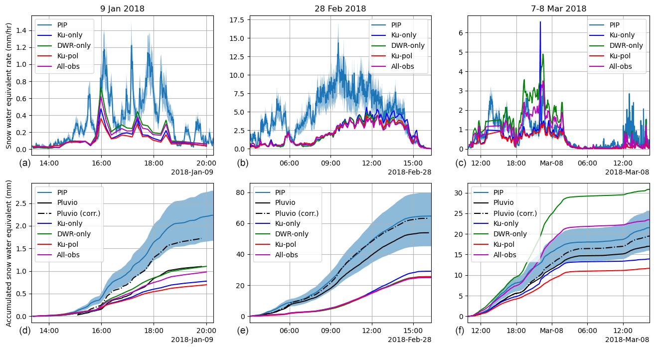
Figure 11Time series of D3R- and PIP-derived snow water equivalent rate (a, b, c) and accumulation (d, e, f) for each event. Because the PIP calculations involve a variety of assumptions to derive particle mass from shape and fall speed (Tokay et al., 2022), a range between the minimum and maximum from these calculations is shaded around the mean PIP-derived value.
Table 7Mean bias, MAE, and correlation coefficient (r) of PIP-derived versus D3R-estimated volumetric snowfall rate (SV) and snow water equivalent rate (S) for each of the four retrieval experiments, compiled over all three events when the D3R-observed Ku-band reflectivity was within the PIP-simulated Ku-band reflectivity range. Because of the wide dynamic range of snowfall rates, these quantities are expressed as percentages relative to the mean PIP estimate.
5.2 Mean particle size and density
The D3R retrieval provides an estimate of the PIP-measured area-weighted mean particle volume diameter (DP) that is consistent with the particle shapes used to generate the LUTs and can be compared directly to the PIP measurement. The time series of this parameter is shown for each event in the top row of Fig. 12. On 9 January 2018, all of the radar retrievals were biased low with respect to the PIP, which is consistent with the reflectivity bias we noted on this day. On 28 February, the PIP measured a rapid increase of DP to a maximum at 06:00 UTC, followed by a decrease to a minimum around 09:00 UTC and another maximum at 15:00 UTC. None of the retrievals did a particularly good job of capturing the peak at 06:00 UTC, but all methods except the Ku-only retrieval captured the increase toward the second maximum, although again, the peak values were underestimated. On 7–8 March, both methods that used the DWR (DWR-only and All-obs) captured the temporal variability of DP quite well but were biased low; this is consistent with a suspected low bias in the DWR for this event (mean cloud-top DWRs were slightly below zero; see Fig. 2).
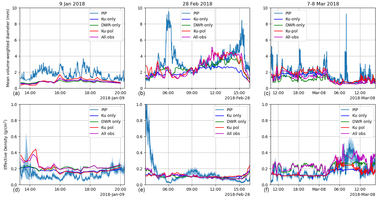
Figure 12Time series of D3R- and PIP-derived mean volume-weighted particle diameter (a, b, c) and effective density (d, e, f) for each event. Because the PIP calculations involve a variety of assumptions to derive particle density from shape and fall speed (Tokay et al., 2022), a range between the minimum and maximum from these calculations is shaded around the mean PIP-derived value.
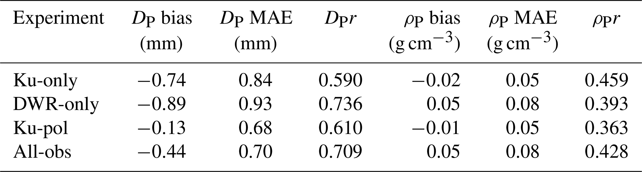
The statistics of the DP retrievals are presented in Table 8 and, as with the snowfall rate statistics, only consider observations where the D3R-observed reflectivity was within the range of calculated PIP values. All of the retrievals are biased low with respect to the PIP, with the Ku-pol retrieval coming the closest. This is counterintuitive, since this retrieval does not consider the DWR, which is the measurement most sensitive to DP. However, the suspected low bias of the DWR on 7–8 March, which dominates the statistics due to its close match to the observed Ku reflectivity, contributes heavily here. The MAE is only slightly lower for the Ku-pol method than the All-obs method, despite the much more significant bias. Meanwhile, the correlation coefficient is largest for the two methods that incorporate the DWR, suggesting that the DWR is indeed informative regarding the particle size; this underscores the need for DWR to be carefully calibrated to avoid significant bias. Combined use of polarimetric and DWR information seems to at least partially alleviate these biases.
The retrieved effective particle density ρP, defined as the snow water equivalent rate divided by the volumetric snowfall rate, can also be directly compared to the PIP measurement (note that this is different from the effective density defined by Pettersen et al., 2020, which is the ratio of fall speeds of an observed snow particle and raindrop of the same equivalent diameter). To first order, ρP is inversely proportional to DP because the unrimed aggregates' density decreases with size. However, changes in fr and fp also affect ρP, so it is worthwhile to evaluate these retrievals as well. The bottom row of Fig. 12 shows the time series of ρP for each event. In general, we find that when the retrieved DP is biased high with respect to the PIP observation, ρP is biased low, and vice versa. It is interesting that on 28 February, all of the D3R methods are in tight agreement, whereas on 7–8 March, the DWR-only and All-obs retrievals are higher than the Ku-only and Ku-pol retrievals, due to the shift toward smaller (denser particles) inferred from the low DWR on this event. In this case, the Ku-only and Ku-pol methods are less biased, but the variability is better represented by the DWR-using retrievals. This is again borne out in the statistics (Table 8), where the Ku-only and Ku-pol methods have the lowest magnitude bias and MAE, and unlike the DP, the Ku-only method has the best correlation (although the All-obs retrieval is the next best). This suggests that the size–density relationship in the scattering models we chose may not be representative of the particles observed during ICE-POP, or that more information (e.g., W-band reflectivity) is needed to constrain the density (e.g., Kneifel et al., 2015).
Table 8Mean bias, absolute error (MAE), and correlation coefficient (r) of PIP-derived versus D3R-estimated mean volume-weighted particle diameter (DvP) and PIP effective density () for each of the four retrieval experiments.
5.3 Bulk particle orientation and aspect ratio
The use of polarimetric measurements in the Ku-pol and All-obs retrievals has the most impact on the retrieved pristine fraction, ratio of pristine to aggregate mean particle size, and pristine population orientation distribution. All of these parameters combine to influence the area-weighted ellipse () and box () aspect ratios. In Fig. 13, the influence of the Zdr and Kdp measurements (Fig. 10) can be observed in these two retrievals, whereas the Ku-only and DWR-only experiments did not appreciably change these parameters. The high Zdr values before 16:00 UTC on 9 January result in low aspect ratios at that time. There is not much of a trend in Zdr on 28 February, due to the constant presence of large aggregates which dominate the Zdr measurement, but there is a notable peak in Kdp around 09:00 UTC which corresponds to the minimum aspect ratio for this event. The 7–8 March event had the least variable polarimetric signatures, but a short peak in Zdr around 18:00 UTC on 7 March corresponds to a drop in aspect ratio at that time.
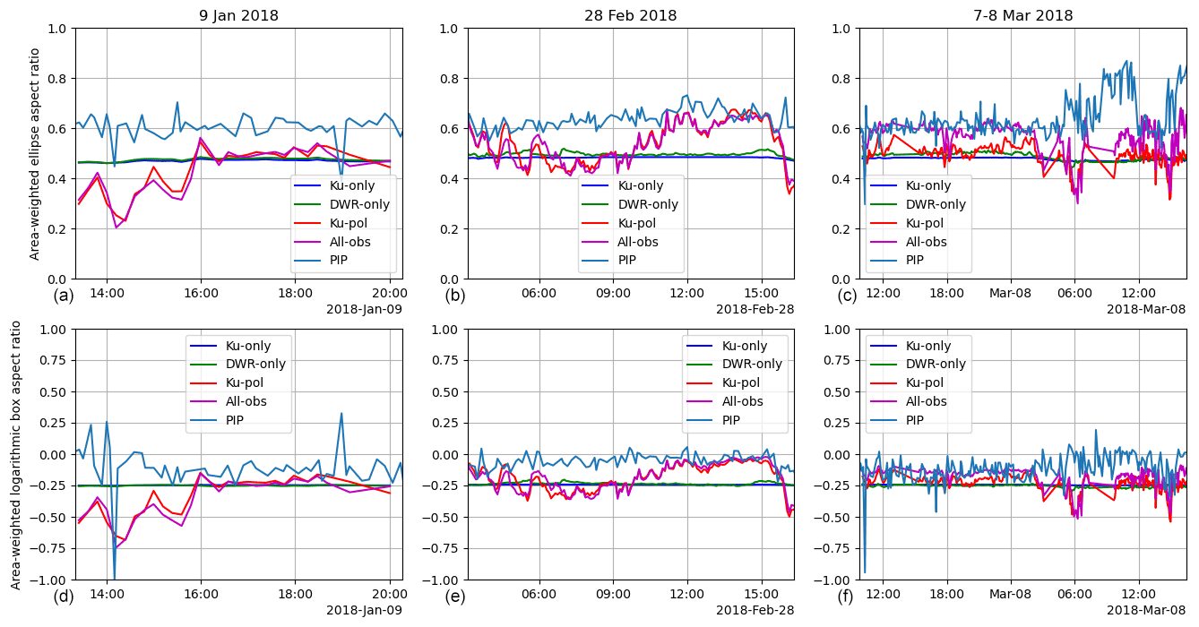
Figure 13Time series of D3R- and PIP-derived area-weighted ellipse (a, b, c) and box (d, e, f) aspect ratio for each event.
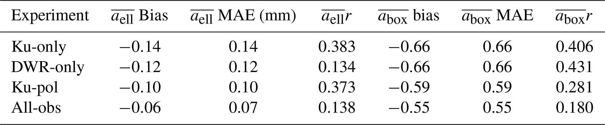
The comparison of the retrieved aspect ratios to those derived from the PIP is inconsistent from event to event. There appears to be little variability in the PIP time series on 9 January for either measure of aspect ratio. There is a steady increase in between 09:00 and 12:00 UTC on 28 February, matching the retrieved behavior, although the PIP range is considerably smaller than the retrieved range. The 7–8 March event does not show any significant trend in the PIP-measured aspect ratios, consistent with the low Zdr variability during this event. The aspect ratio error statistics are given in Table 9. The Ku-pol and All-obs methods provide the lowest MAE and least bias; however, the best correlation comes from the Ku-only method (for ) and the DWR-only method (for ). This is a surprising result, especially in light of the very small range of these retrieved values in Fig. 13. In these methods, the very limited aspect ratio variability is entirely driven by changes in PSD, with smaller mean particle sizes being associated with smaller aspect ratios. The polarimetric measurements add significant variation to the retrieved aspect ratio, but the correlation statistics suggest that the relationship between these measurement and PIP-derived aspect ratio and orientation is tenuous at best. Helms et al. (2022) provide further information on the algorithms used to derive aspect ratio and orientation from the PIP; noting that motion blurring and compression lead to artificially high aspect ratios, particularly for small particles, and quantization artifacts that lead to a maximum aspect ratio of 0.6 for particles less than 0.5 mm in diameter. In future deployments, we expect to measure these properties more precisely as these algorithms improve, and co-located high-resolution cameras (such as the Multi-Angle Snowflake Camera instrument; Garrett et al., 2012) provide complementary information about selected individual particles, while the PIP, with its wider field of view, provides more information about the PSD and bulk snowfall properties.
Table 9Mean bias, absolute error (MAE), and correlation coefficient (r) of PIP-derived versus D3R-estimated mean area-weighted ellipse () and box () aspect ratio for each of the four retrieval experiments.
This study describes an algorithm that makes use of both polarimetric and dual-frequency radar measurements to retrieve microphysical properties of falling snow, including snowfall rate (volumetric and water equivalent); ice water content; particle size distribution; the relative contribution of pristine, aggregate, and rimed species; and particle orientation distribution. The algorithm is flexible in that it can use as many or as few measurements as available. In this study, it is applied to the Ku- and Ka-band measurements of the NASA D3R radar obtained during the ICE-POP 2018 field campaign but can be applied to additional or different frequencies. This is possible because it makes use of the ARTS microwave single-scattering property database for oriented particles (Brath et al., 2020), which encompasses ADDA (Yurkin and Hoekstra, 2011) scattering calculations over a wide range of frequencies. This differentiates it from methods that use T-matrix or Rayleigh–Gans approximations but constrains it to use the particle geometries that are available (at this time, only hexagonal plates and aggregates composed of these plates). More geometries are available for randomly oriented particles, but these cannot make use of the polarimetric information (although they are used in this study to represent the rimed particles).
The retrieval uses optimal estimation to solve for several parameters that describe the PSD, relative contribution of each species, and the orientation distribution along an entire radial simultaneously. This is necessary (versus a gate-by-gate approach) to account for the measurements sensitive to propagation effects (e.g., DWR and ϕdp). Examination of Jacobian matrices and averaging kernels shows that the DWR provides information regarding the characteristic particle size, and to a lesser extent, the rime fraction and shape parameter of the size distribution. The Zdr measurements provide information regarding the mass fraction of pristine particles and their characteristic size and orientation distribution. Meanwhile, the ϕdp measurements are sensitive to most of the same measurements as Zdr but are also sensitive to the overall particle concentration. Thus, by combining the dual-frequency and polarimetric measurements, some ambiguities can be resolved that should allow a better determination of the particle size distribution parameters and integrated quantities (e.g., ice water content, snowfall rate) than can be retrieved from single-frequency polarimetric measurements or dual-frequency, single-polarization measurements.
The D3R ICE-POP retrievals were validated using PIP and Pluvio measurements taken nearby at the May Hills ground site. The PIP measures the snow PSD directly (Pettersen et al., 2020) and several useful parameters can be derived directly from its measurements or indirectly with additional assumptions. These include the snowfall rate (volumetric and water equivalent), mean volume-weighted particle size, and effective density (Tokay et al., 2022), as well as parameters describing the mean aspect ratio and orientation distribution. We validated the retrieval during three events representing both warm and cold snow regimes (Kim et al., 2021). These events were chosen based upon availability of both PIP and D3R data, significant accumulation at the MHS location, and absence of any mixed-phase precipitation which the algorithm does not account for. Four retrieval experiments were performed to evaluate the utility of different measurement combinations: Ku-only, DWR-only, Ku-pol, and All-obs. In terms of mean absolute error and correlation, the volumetric snowfall rate was best retrieved (r=0.95), followed closely by the snow water equivalent rate (r=0.92). The Ku-pol method had the highest correlation to these parameters, while the DWR-only and All-obs methods had the lowest magnitude bias. These methods that incorporated DWR also had the best correlation to particle size (r=0.74), although none of the methods retrieved density particularly well (r=0.46). The ability of the measurements to retrieve mean aspect ratio was also inconclusive, although the polarimetric methods (Ku-pol and All-obs) had reduced biases and MAE relative to the Ku-only and DWR-only methods. The significant biases in particle size and snowfall rate appeared to be related to biases in the measured DWR (positive on 28 February and negative on 7–8 March), emphasizing the need for accurate DWR measurements and frequent calibration (e.g., co-located measurements at a non-attenuating frequency such as S or C band). Notwithstanding these calibration biases, during the most well-behaved event (7–8 March), where the PIP-derived reflectivity was closest to the D3R measurement, the All-obs method provided the best snowfall accumulation and closely approximated the observed time series of snowfall rate and particle size.
The D3R is scheduled to be deployed in Storrs, Connecticut, USA, during the 2021–2022 and 2022–2023 winters as part of the NASA-sponsored Investigation of Microphysics and Precipitation for Atlantic Coast-Threatening Snowstorms (IMPACTS) field experiment. A similar deployment setup is planned with nearby PIP measurements. Additionally, the airborne Ku- and Ka-band HIWRAP radar will be available to evaluate the D3R calibration, and other lessons learned (e.g., video monitoring to observe snow accumulation on the radome, siting to avoid ground clutter) will be applied. Ongoing improvements to the PIP processing algorithms, particularly regarding the estimation of particle aspect ratio, will also be advantageous to further refine the algorithm described in this work. Availability of scattering databases for oriented particles with different geometries will facilitate running these retrievals as an ensemble to provide more robust posterior distributions of the retrieved parameters. Finally, the methodology can be expanded to accommodate liquid and melting particles, although scattering databases for the latter, particularly with the polarimetric parameters from oriented melting particles, are not yet mature enough for this application.
Faithfully simulating the observables from polarimetric radar requires considering the incident and scattered Stokes vectors; these vectors are related via (Adams and Bettenhausen, 2012)
where I, Q, U, and V are the elements of the Stokes vector, r is the distance from the sensor to the particle, Zlm are the elements of the scattering or phase matrix, and the i and s subscripts indicate incidence and scattering, respectively.
To generate tables of the polarimetric, single-scattering properties, we transform the Stokes matrix elements to single-scattering properties more commonly used in radar meteorology, such as backscatter cross section at horizontal and vertical polarizations ( and , respectively). Additionally, we include the complex, co-polar conjugate product Chv between the scattering amplitude matrix elements at horizontal and vertical polarization (Shh and Svv, respectively) that allow for the co-polar correlation coefficient ρhv to be calculated. These variables are defined in terms of the phase matrix elements as (Ekelund et al., 2020)
All the expressions above define the phase matrix elements as in the backscatter direction, or opposite the incident direction, and the phase matrix elements have units of mm2.
Expressions are given below for the radar reflectivity factor
in units of mm6 m−3 and co-polar correlation coefficient
The propagation variables, Kdp, and the extinction cross sections ( and ) can be calculated from the corresponding extinction matrix of the particle. The oriented, azimuthally random uniform particles we use from the ARTS database have only three independent extinction matrix elements: K11, K12, and K34. The propagation variables are thus defined as (Ekelund et al., 2020)
The extinction matrix elements have units of mm2 and Kdp has units of degree km−1.
The D3R measurements that comprise the observation vector Y (Eq. 12) are forward modeled from the measured Ku-band vertically polarized reflectivity 1 and the state vector X. This combination of frequency and polarization was chosen because it is least prone to error in the attenuation correction. To simulate the D3R measurements, we must obtain both the backscattering properties of the ice particles as well as the propagation scattering properties (i.e., the propagation phase shifts and attenuation at each polarization) from the LUTs defined in Sect. 3. The components of Y are defined by the following equations that include the propagation effects along a radial:
where Kdp(f) is the specific differential phase at frequency f, ϕsys is the system differential phase upon transmission, and is the attenuated reflectivity at polarization p and frequency f defined as
Here, is the intrinsic effective reflectivity factor and kext(p,f) is the specific attenuation, which includes contributions from gases, cloud liquid water, and hydrometeors. The symbols p and f indicate the polarization and frequency, respectively.
DWR, Zdr, and ϕdp are forward simulated from Eqs. (B1)–(B4) by integrating numerically along each radial, following a conceptually similar process to that of Grecu et al. (2011). First, at each range gate, the attenuation contributions from gases (determined by the closest-in-time sounding from DGW) and cloud liquid (part of the retrieval state vector) are calculated. Next, is calculated by inserting the observed and the calculated two-way path-integrated attenuation from previous range gates into Eq. (B4). Then, , kext(p,f), and Kdp(f), along with the simulated PIP measurements in Table 4, are calculated from interpolated LUTs that have been combined for all the species according to the retrieval parameters and scaled to the observed . These quantities are then used to forward model the measurements that comprise Y following Eqs. (B1)–(B4).
The process of simulating the radar measurements from combined LUTs can be described by considering a LUT for a variable V selected from Table 4. First, the LUT dimensionality for each species is reduced by linear interpolation over the following parameters: the radial zenith angle θ, temperature at the altitude of the range gate, and species-specific μ and κ values interpolated from the nodes for these parameters. At this stage, the remaining LUT dimensions are Dm and frequency (for the radar variables). Next, the unrimed aggregate (Vu) and rimed (Vr) LUTs are combined into a merged “aggregate” LUT (Va) by weighting each species according to the rime mass fraction interpolated to each range gate r:
Recall from Sect. 3 that the LUTs are normalized to contain a constant 1 g m−3 ice water content; there exists a corresponding value consistent with that water content. Because is prescribed at each range gate from the interpolated retrieval parameter (see definition in Table 5), the LUT for each species s is rescaled element wise to be consistent with this prescribed :
The pristine and aggregate LUTs are then merged – individually for the scaled and unscaled LUTs – according to the interpolated retrieval parameters fp (pristine mass fraction) and Dp (ratio of the pristine to aggregate Dm). To perform this merging, first the mean mass-weighted diameter dimension of the combined LUT (Dm,c) is calculated from the prescribed fp, Dp, and aggregate Dm,a:
Next, the variables in the pristine LUTs (Vp and ) are interpolated to this new set of Dm,c values and merged with the aggregate LUTs (Va and ) according to the prescribed mass fraction to create a combined LUT:
Now there exists a one-dimensional LUT for each parameter (and frequency for the radar variables) that is indexed by Dm and is consistent with the prescribed PSD characteristics from the retrieval state vector. The retrieved value of Dm(r) is that which produces the attenuation-corrected (from Eq. B4 over prior range gates) from the -scaled Zv,Ku LUT. From this retrieved Dm(r), the ice water content W(r) (in g m−3) is simply the scaling factor that is required to produce this from the unscaled LUT. Once Dm(r) and W(r) are determined, all of the remaining LUT parameters, including those needed to simulate the measurements in Y as well as the simulated PIP measurements used for validation, can be readily calculated by interpolating the LUTs to Dm(r) and scaling by W(r). These parameters are saved to the output data structure, and the propagation equations are iteratively integrated to repeat the process at the next range gate.
The D3R data used in this study (Chandrasekar, 2019) can be accessed at https://doi.org/10.5067/GPMGV/ICEPOP/D3R/DATA101. The PIP data (Bliven, 2020) can be accessed at https://doi.org/10.5067/GPMGV/ICEPOP/PIP/DATA101.
SJM led this research by developing the lookup tables and optimal estimation methodology, processing the radar data, and calculating validation statistics. RSS assisted with the generation of lookup tables, polarimetric components of the radar forward model, and assessment of forward model error. AT processed the PIP and Pluvio measurements that were used for validation. CNH performed additional processing of the PIP data to derive the bulk aspect ratio and orientation parameters.
At least one of the (co-)authors is a member of the editorial board of Atmospheric Measurement Techniques. The peer-review process was guided by an independent editor, and the authors also have no other competing interests to declare.
Publisher’s note: Copernicus Publications remains neutral with regard to jurisdictional claims in published maps and institutional affiliations.
This article is part of the special issue “Winter weather research in complex terrain during ICE-POP 2018 (International Collaborative Experiments for PyeongChang 2018 Olympic and Paralympic winter games) (ACP/AMT/GMD inter-journal SI)”. It is not associated with a conference.
Robert S. Schrom's and Charles N. Helms' work was supported by an appointment to the NASA Postdoctoral Program at NASA Goddard Space Flight Center, administered by Universities Space Research Association under contract with NASA. S. Joseph Munchak and Ali Tokay were supported by the Global Precipitation Measurement (GPM) Ground Validation program. The authors would also like to acknowledge many insightful discussions about the D3R data quality and calibration procedures with Venkatachalam Chandrasekhar at Colorado State University. The authors greatly appreciate the participants in the World Weather Research Programme Research Development Project and Forecast Demonstration Project, International Collaborative Experiments for PyeongChang 2018 Olympic and Paralympic winter games (ICE-POP 2018), hosted by Korea Meteorological Administration (KMA), and would like to acknowledge GyuWon Lee of Kyungpook National University, Daegu, South Korea, for stimulating ongoing scientific research from datasets collected during ICE-POP 2018.
This research has been supported by the National Aeronautics and Space Administration (Internal Scientist Funding Model Work Package: GPM Ground Validation).
This paper was edited by GyuWon Lee and reviewed by two anonymous referees.
Adams, I. S. and Bettenhausen, M. H.: The scattering properties of horizontally aligned snow crystals and crystal approximations at millimeter wavelengths, Radio Sci., 47, RS5007, https://doi.org/10.1029/2012RS005015, 2012. a
Andrić, J., Kumjian, M. R., Zrnić, D. S., Straka, J. M., and Melnikov, V. M.: Polarimetric signatures above the melting layer in winter storms: An observational and modeling study, J. Appl. Meteorol. Clim., 52, 682–700, 2013. a
Beard, K. V., Bringi, V., and Thurai, M.: A new understanding of raindrop shape, Atmos. Res., 97, 396–415, https://doi.org/10.1016/j.atmosres.2010.02.001, 2010. a
Bechini, R., Baldini, L., and Chandrasekar, V.: Polarimetric radar observations in the ice region of precipitating clouds at C-band and X-band radar frequencies, J. Appl. Meteorol. Clim., 52, 1147–1169, 2013. a, b
Bliven, L.: GPM Ground Validation Precipitation Imaging Package (PIP) ICE POP, NASA Global Hydrology Resource Center DAAC [data set], Huntsville, Alabama, USA, https://doi.org/10.5067/GPMGV/ICEPOP/PIP/DATA101, 2020. a
Botta, G., Aydin, K., and Verlinde, J.: Variability in millimeter wave scattering properties of dendritic ice crystals, J. Quant. Spectrosc. Ra., 131, 105–114, 2013. a
Brath, M., Ekelund, R., Eriksson, P., Lemke, O., and Buehler, S. A.: Microwave and submillimeter wave scattering of oriented ice particles, Atmos. Meas. Tech., 13, 2309–2333, https://doi.org/10.5194/amt-13-2309-2020, 2020. a, b, c
Bringi, V. N. and Chandrasekar, V.: Polarimetric Doppler Weather Radar, Cambridge University Press, 1st edn., ISBN 0521623847, 2001. a
Bukovčić, P., Ryzhkov, A., and Zrnić, D.: Polarimetric relations for snow estimation–radar verification, J. Appl. Meteorol. Clim., 59, 991–1009, 2020. a
Chandrasekar, V., Schwaller, M., Vega, M., Carswell, J., Mishra, K. V., Meneghini, R., and Nguyen, C.: Scientific and engineering overview of the NASA Dual-Frequency Dual-Polarized Doppler Radar (D3R) system for GPM Ground Validation, in: 2010 IEEE International Geoscience and Remote Sensing Symposium, Honolulu, HI, USA, 25–30 July 2010, IEEE, 1308–1311, https://doi.org/10.1109/IGARSS.2010.5649440, 2010. a, b
Chandrasekar, V., Vega, M. A., Joshil, S., Kumar, M., Wolff, D., and Petersen, W.: Deployment and performance of the nasa d3r during the ice-pop 2018 field campaign in South Korea, in: IGARSS 2018-2018 IEEE International Geoscience and Remote Sensing Symposium, Valencia, Spain, 22–27 July 2018, IEEE, 8349–8351, https://doi.org/10.1109/IGARSS.2018.8517313, 2018. a
Chandrasekar, V.: GPM Ground Validation Dual-frequency Dual-polarized Doppler Radar (D3R) ICE POP, NASA Global Hydrology Resource Center DAAC [data set], Huntsville, Alabama, USA, https://doi.org/10.5067/GPMGV/ICEPOP/D3R/DATA101, 2019. a
Chase, R. J., Finlon, J. A., Borque, P., McFarquhar, G. M., Nesbitt, S. W., Tanelli, S., Sy, O. O., Durden, S. L., and Poellot, M. R.: Evaluation of triple-frequency radar retrieval of snowfall properties using coincident airborne in situ observations during OLYMPEX, Geophys. Res. Lett., 45, 5752–5760, 2018. a
Chase, R. J., Nesbitt, S. W., and McFarquhar, G. M.: A Dual-Frequency Radar Retrieval of Two Parameters of the Snowfall Particle Size Distribution Using a Neural Network, J. Appl. Meteorol. Clim., 60, 341–359, 2021. a
Chen, J. and Lamb, D.: The theoretical basis for the parametrerization of ice crystal habits: Growth by vapor deposition, J. Atmos. Sci., 51, 1206–1222, 1994. a
Connolly, P. J., Emersic, C., and Field, P. R.: A laboratory investigation into the aggregation efficiency of small ice crystals, Atmos. Chem. Phys., 12, 2055–2076, https://doi.org/10.5194/acp-12-2055-2012, 2012. a
de Boer, G., Ivey, M., Schmid, B., Lawrence, D., Dexheimer, D., Mei, F., Hubbe, J., Bendure, A., Hardesty, J., Shupe, M. D., McComiskey, A., Telg, H., Schmitt, C., Matrosov, S. Y., Brooks, I., Creamean, J., Solomon, A., Turner, D. D., Williams, C., Maahn, M., Argrow, B., Palo, S., Long, C. N., Gao, R., and Mather, J.: A bird’s eye view: Development of an operational ARM unmanned aerial capability for atmospheric research in Arctic Alaska, B. Am. Meteorol. Soc., 99, 1197–1212, 2018. a
Ekelund, R., Eriksson, P., and Kahnert, M.: Microwave single-scattering properties of non-spheroidal raindrops, Atmos. Meas. Tech., 13, 6933–6944, https://doi.org/10.5194/amt-13-6933-2020, 2020. a, b, c, d
Eriksson, P., Ekelund, R., Mendrok, J., Brath, M., Lemke, O., and Buehler, S. A.: A general database of hydrometeor single scattering properties at microwave and sub-millimetre wavelengths, Earth Syst. Sci. Data, 10, 1301–1326, https://doi.org/10.5194/essd-10-1301-2018, 2018. a
Field, P., Hogan, R., Brown, P., Illingworth, A., Choularton, T., and Cotton, R.: Parametrization of ice-particle size distributions for mid-latitude stratiform cloud, Q. J. Roy. Meteorol. Soc., 131, 1997–2017, 2005. a, b
Fukuta, N. and Takahashi, T.: The growth of atmospheric ice crystals: A summary of findings in vertical supercooled cloud tunnel studies, J. Atmos. Sci., 56, 1963–1979, 1999. a
Garrett, T. J., Fallgatter, C., Shkurko, K., and Howlett, D.: Fall speed measurement and high-resolution multi-angle photography of hydrometeors in free fall, Atmos. Meas. Tech., 5, 2625–2633, https://doi.org/10.5194/amt-5-2625-2012, 2012. a
Grecu, M., Tian, L., Olson, W. S., and Tanelli, S.: A robust dual-frequency radar profiling algorithm, J. Appl. Meteorol. Clim., 50, 1543–1557, 2011. a, b, c
Hall, M. P. M., Goddard, J. W. F., and Cherry, S. M.: Identification of hydrometeors and other targets by dual-polarization radar, Radio Sci., 19, 132–140, 1984. a
Hari, P. and Kulmala, M.: Station for Measuring Ecosystem–Atmosphere Relations (SMEAR II), Boreal Environ. Res., 10, 315–322, 2005. a
Helms, C. N., Munchak, S. J., Tokay, A., and Pettersen, C.: A Comparative Evaluation of Snowflake Particle Size and Shape Estimation Techniques used by the Precipitation Imaging Package (PIP), Multi-Angle Snowflake Camera (MASC), and Two-Dimensional Video Disdrometer (2DVD), Atmos. Meas. Tech. Discuss. [preprint], https://doi.org/10.5194/amt-2021-427, in review, 2022. a, b
Heymsfield, A. J. and Westbrook, C. D.: Advances in the estimation of ice particle fall speeds using laboratory and field measurements, J. Atmos. Sci., 67, 2469–2482, 2010. a, b
Hobbs, P. V., Chang, S., and Locatelli, J. D.: The dimensions and aggregation of ice crystals in natural clouds, J. Geophys. Res., 79, 2199–2206, 1974. a
Hosler, C. L., Jensen, D. C., and Goldshlak, L.: On the aggregation of ice crystals to form snow, Journal of Operational Meteorology, 14, 415–420, 1957. a
Jensen, A. A. and Harrington, J. Y.: Modeling ice crystal aspect ratio evolution during riming: A single-particle growth model, J. Atmos. Sci., 72, 2569–2590, 2015. a
Jiang, Z., Oue, M., Verlinde, J., Clothiaux, E. E., Aydin, K., Botta, G., and Lu, Y.: What can we conclude about the real aspect ratios of ice particle aggregates from two-dimensional images?, J. Appl. Meteorol. Clim., 56, 725–734, 2017. a
Kennedy, P. C. and Rutledge, S. A.: S-band dual-polarization radar observations of winter storms, J. Appl. Meteorol. Clim., 50, 844–858, 2011. a
Kim, K., Bang, W., Chang, E.-C., Tapiador, F. J., Tsai, C.-L., Jung, E., and Lee, G.: Impact of wind pattern and complex topography on snow microphysics during International Collaborative Experiment for PyeongChang 2018 Olympic and Paralympic winter games (ICE-POP 2018), Atmos. Chem. Phys., 21, 11955–11978, https://doi.org/10.5194/acp-21-11955-2021, 2021. a, b
Klett, J. D.: Orientation model for particles in turbulence, J. Atmos. Sci., 52, 2276–2285, 1995. a
Kneifel, S., von Lerber, A., Tiira, J., Moisseev, D., Kollias, P., and Leinonen, J.: Observed relations between snowfall microphysics and triple-frequency radar measurements, J. Geophys. Res.-Atmos., 120, 6034–6055, 2015. a, b
Kumar, M., Joshil, S. S., Chandrasekar, V., Beauchamp, R. M., Vega, M., and Zebley, J. W.: Performance trade-offs and upgrade of NASA D3R weather radar, in: 2017 IEEE International Geoscience and Remote Sensing Symposium (IGARSS), Fort Worth, TX, USA, 23–28 July 2017, 5260–5263, https://doi.org/10.1109/IGARSS.2017.8128188, 2017. a, b
Kumjian, M. R.: Principles and applications of dual-polarization weather radar. Part I: Description of the polarimetric radar variables, Journal of Operational Meteorology, 1, 226–242, 2013. a
Kumjian, M. R. and Lombardo, K. A.: Insights into the evolving microphysical and kinematic structure of northeastern U.S. winter storms from dual-polarization Doppler radar, Mon. Weather Rev., 145, 1033–1061, 2017. a
Kuo, K., Olson, W. S., Johnson, B. T., Grecu, M., Tian, L., Clune, T. L., van Aartsen, B. H., Heymsfield, A. J., Liao, L., and Meneghini, R.: The microwave radiative properties of falling snow derived from nonspherical ice particle models. Part I: An extensive database of simulated pristine crystals and aggregate particles, and their scattering properties, J. Appl. Meteorol. Clim., 56, 691–708, 2016. a
Kuroda, T. and Lacmann, R.: Growth kinetics of ice from the vapour phase and its growth forms, J. Cryst. Growth, 56, 189–205, 1982. a
L'Ecuyer, T. S. and Stephens, G. L.: An estimation-based precipitation retrieval algorithm for attenuating radars, J. Appl. Meteorol., 41, 272–285, 2002. a
Leinonen, J. and von Lerber, A.: Snowflake melting simulation using smoothed particle hydrodynamics, J. Geophys. Res.-Atmos., 123, 1811–1825, 2018. a
Leinonen, J., Lebsock, M. D., Tanelli, S., Sy, O. O., Dolan, B., Chase, R. J., Finlon, J. A., von Lerber, A., and Moisseev, D.: Retrieval of snowflake microphysical properties from multifrequency radar observations, Atmos. Meas. Tech., 11, 5471–5488, https://doi.org/10.5194/amt-11-5471-2018, 2018. a
Liao, L., Meneghini, R., Tokay, A., and Bliven, L. F.: Retrieval of snow properties for Ku-and Ka-band dual-frequency radar, J. Appl. Meteorol. Clim., 55, 1845–1858, 2016. a
Lim, K.-S. S., Chang, E.-C., Sun, R., Kim, K., Tapiador, F. J., and Lee, G.: Evaluation of simulated winter precipitation using WRF-ARW during the ICE-POP 2018 field campaign, Weather Forecast., 35, 2199–2213, 2020. a
Löhnert, U., Schween, J. H., Acquistapace, C., Ebell, K., Maahn, M., Barrera-Verdejo, M., Hirsikko, A., Bohn, B., Knaps, A., O’Connor, E., Simmer, C., Wahner, A., and Crewell, S.: JOYCE: Jülich Observatory for Cloud Evolution, B. Am. Meteorol. Soc., 96, 1157–1174, https://doi.org/10.1175/BAMS-D-14-00105.1, 2015. a
Marshall, J. S. and Gunn, K. L. S.: The microwave properties of precipitation particles, J. Atmos. Sci., 9, 322–327, 1952. a
Mason, S., Chiu, C., Hogan, R., Moisseev, D., and Kneifel, S.: Retrievals of riming and snow density from vertically pointing Doppler radars, J. Geophys. Res.-Atmos., 123, 13807–13834, 2018. a, b
Matrosov, S. Y., Heymsfield, A., and Wang, Z.: Dual-frequency radar ratio of nonspherical atmospheric hydrometeors, Geophys. Res. Lett., 32, L13816, https://doi.org/10.1029/2005GL023210, 2005. a
Matsuo, T. and Sasyo, Y.: Empirical formula for the melting rate of snowflakes, J. Meteorol. Soc. Jpn., Ser. II, 59, 1–9, 1981. a
Melnikov, V. and Straka, J. M.: Axis ratios and flutter angles of cloud ice particles: Retrievals from radar data, J. Atmos. Ocean. Tech., 30, 1691–1703, 2013. a
Meteomodem: Meteomodem M10 Radiosonde Information Leaflet, http://www.meteomodem.com/docs/en/Leaflet-m10.pdf (last access: 4 March 2022), 2021. a
Milewska, E. J., Vincent, L. A., Hartwell, M. M., Charlesworth, K., and Mekis, É.: Adjusting precipitation amounts from Geonor and Pluvio automated weighing gauges to preserve continuity of observations in Canada, Can. Water Resour. J., 44, 127–145, 2019. a
Mitchell, D. L., Zhang, R., and Pitter, R. L.: Mass-Dimensional Relationships for Ice Particles and the Influence of Riming on Snowfall Rates, J. Appl. Meteorol. Clim., 29, 153–163, https://doi.org/10.1175/1520-0450(1990)029<0153:MDRFIP>2.0.CO;2, 1990. a
Moisseev, D., von Lerber, A., and Tiira, J.: Quantifying the effect of riming on snowfall using ground-based observations, J. Geophys. Res.-Atmos., 122, 4019–4037, https://doi.org/10.1002/2016JD026272, 2017. a
Moisseev, D. N., Lautaportti, S., Tyynela, J., and Lim, S.: Dual-polarization radar signatures in snowstorms: Role of snowflake aggregation, J. Geophys. Res., 120, 12644–12655, 2015. a
Munchak, S. J. and Kummerow, C. D.: A modular optimal estimation method for combined radar–radiometer precipitation profiling, J. Appl. Meteorol. Clim., 50, 433–448, 2011. a
Oue, M., Kumjian, M. R., Lu, Y., Jiang, Z., Clothiaux, E. E., Verlinde, J., and Aydin, K.: X-band polarimetric and Ka-band Doppler spectral radar observations of a graupel-producing Arctic mixed-phase cloud, J. Appl. Meteorol. Climatol., 54, 1335–1351, 2015. a, b
Petersen, W., Wolff, D., Zavodsky, B., and Roberts, J.: International Collaborative Experiment for PyeongChang Olympic and Paralympics (ICE-POP) Collection, NASA EOSDIS Global Hydrology Resource Center Distributed Active Archive Center [data set], Huntsville, Alabama, USA, https://doi.org/10.5067/GPMGV/ICEPOP/DATA101, 2018. a
Pettersen, C., Bliven, L. F., von Lerber, A., Wood, N. B., Kulie, M. S., Mateling, M. E., Moisseev, D. N., Munchak, S. J., Petersen, W. A., and Wolff, D. B.: The precipitation imaging package: Assessment of microphysical and bulk characteristics of snow, Atmosphere, 11, 785, https://doi.org/10.3390/atmos11080785, 2020. a, b, c
Petty, G. W. and Huang, W.: The modified gamma size distribution applied to inhomogeneous and nonspherical particles: Key relationships and conversions, J. Atmos. Sci., 68, 1460–1473, 2011. a
Rodgers, C. D.: Inverse methods for atmospheric sounding: theory and practice, vol. 2, World scientific, ISBN 981022740X, 2000. a
Ryzhkov, A. V. and Zrnić, D. S.: Discrimination between rain and snow with a polarimetric radar, J. Appl. Meteorol., 37, 1228–1240, 1998. a
Ryzhkov, A. V., Zhang, P., Reeves, H. D., Kumjian, M. R., Tschallener, T., Troemel, S., and Simmer, C.: Quasi-vertical profiles – a new way to look at polarimetric radar data, J. Atmos. Ocean. Tech., 33, 551–562, 2016. a
Schrom, R. S. and Kumjian, M. R.: Connecting microphysical processes in Colorado winter storms with vertical profiles of radar observations, J. Appl. Meteorol. Clim., 55, 1771–1787, 2016. a
Schrom, R. S., Kumjian, M. R., and Lu, Y.: Polarimetric radar observations of dendritic growth zones in Colorado winter storms, J. Appl. Meteorol. Clim., 54, 2365–2388, 2015. a
Schrom, R. S., van Lier-Walqui, M., Kumjian, M. R., Harrington, J. Y., Jensen, A. A., and Chen, Y.: Radar-based Bayesian estimation of ice crystal growth parameters within a microphysical model, J. Atmos. Sci., 78, 549–569, 2021. a, b
Skofronick-Jackson, G., Hudak, D., Petersen, W., Nesbitt, S. W., Chandrasekar, V., Durden, S., Gleicher, K. J., Huang, G.-J., Joe, P., Kollias, P., Reed, K. A., Schwaller, M. R., Stewart, R., Tanelli, S., Tokay, A., Wang, J. R., and Wolde, M.: Global precipitation measurement cold season precipitation experiment (GCPEX): For measurement’s sake, let it snow, B. Am. Meteorol. Soc., 96, 1719–1741, 2015. a
Skofronick-Jackson, G., Kulie, M., Milani, L., Munchak, S. J., Wood, N. B., and Levizzani, V.: Satellite estimation of falling snow: A global precipitation measurement (GPM) core observatory perspective, J. Appl. Meteorol. Clim., 58, 1429–1448, 2019. a
Smith, A. J., Larson, V. E., Niu, J., Kankiewicz, J. A., and Carey, L. D.: Processes that generate and deplete liquid water and snow in thin midlevel mixed-phase clouds, J. Geophys. Res., 114, D12203, https://doi.org/10.1029/2008JD011531, 2009. a
Thompson, E. J., Rutledge, S. A., Dolan, B., Chandrasekar, V., and Cheong, B.: A dual-polarization radar hydrometeor classification algorithm for winter precipitation, J. Atmos. Ocean. Tech., 31, 1457–1481, 2014. a
Tiira, J., Moisseev, D. N., von Lerber, A., Ori, D., Tokay, A., Bliven, L. F., and Petersen, W.: Ensemble mean density and its connection to other microphysical properties of falling snow as observed in Southern Finland, Atmos. Meas. Tech., 9, 4825–4841, https://doi.org/10.5194/amt-9-4825-2016, 2016. a
Tokay, A., Liao, L., Meneghini, R., Helms, C., Munchak, S. J., Gatlin, P. N., and Wolff, D. B.: Retrieval of Normalized Gamma Size Distribution Parameters using Precipitation Imaging Package (PIP) Observations during ICE-POP, J. Appl. Meteorol. Clim., in review, 2022. a, b, c, d, e, f
Tridon, F., Battaglia, A., Chase, R. J., Turk, F. J., Leinonen, J., Kneifel, S., Mroz, K., Finlon, J., Bansemer, A., Tanelli, S., Heymsfield, A. J., and Nesbitt, S. W.: The microphysics of stratiform precipitation during OLYMPEX: Compatibility between triple-frequency radar and airborne in situ observations, J. Geophys. Res.-Atmos., 124, 8764–8792, 2019. a
Vega, M. A., Chandrasekar, V., Carswell, J., Beauchamp, R. M., Schwaller, M. R., and Nguyen, C.: Salient features of the dual-frequency, dual-polarized, Doppler radar for remote sensing of precipitation, Radio Sci., 49, 1087–1105, https://doi.org/10.1002/2014RS005529, 2014. a
Vivekanandan, J., Bringi, V. N., Hagen, M., and Meischner, P.: Polarimetric radar studies of atmospheric ice particles, IEEE T. Geosci. Remote, 32, 1–10, 1994. a
Yurkin, M. A. and Hoekstra, A. G.: The discrete-dipole-approximation code ADDA: Capabilities and known limitations, J. Quant. Spectrosc. Ra., 112, 2234–2247, 2011. a
Reflectivity is defined in linear units in this appendix unless otherwise noted.
- Abstract
- Introduction
- Datasets
- Particle scattering properties
- Algorithm description
- Validation
- Conclusions
- Appendix A: Derivation of single-scattering properties
- Appendix B: Radar forward model
- Data availability
- Author contributions
- Competing interests
- Disclaimer
- Special issue statement
- Acknowledgements
- Financial support
- Review statement
- References