the Creative Commons Attribution 4.0 License.
the Creative Commons Attribution 4.0 License.
 | 17 Mar 2022
Remote sensing of solar surface radiation – a reflection of concepts, applications and input data based on experience with the effective cloud albedo
Uwe Pfeifroth
Accurate solar surface irradiance (SSI) data are a prerequisite for efficient planning and operation of solar energy systems. Respective data are also essential for climate monitoring and analysis. Satellite-based SSI has grown in importance over the last few decades. However, a retrieval method is needed to relate the measured radiances at the satellite to the solar surface irradiance. In a widespread classical approach, these radiances are used directly to derive the effective cloud albedo (CAL) as basis for the estimation of the solar surface irradiance. This approach was already introduced and discussed in the early 1980s. Various approaches are briefly discussed and analysed, including an overview of open questions and opportunities for improvement. Special emphasis is placed on the reflection of fundamental physical laws and atmospheric measurement techniques. In addition, atmospheric input data and key applications are briefly discussed. It is concluded that the well-established observation-based CAL approach is still an excellent choice for the retrieval of the cloud transmission. The coupling with lookup-table-based clear-sky models enables the estimation of solar surface irradiance with high accuracy and homogeneity. This could explain why, despite its age, the direct CAL approach is still used by key players in energy meteorology and the climate community. For the clear-sky input data, it is recommended to use ECMWF forecast and reanalysis data.
- Article
(489 KB) - Full-text XML
- BibTeX
- EndNote


The surface solar irradiance (SSI) is defined as the incoming solar radiation at the surface in the 0.2–4.0 µm wavelength region on a given surface area and is usually expressed in W m−2 (watts per square metre). SSI consists of the diffuse part (diffuse irradiance) and the direct part (direct irradiance), which is received from the direction of the Sun. Diffuse radiation results from scattering by the atmosphere and is received from all directions.
Solar irradiance is a forcing quantity for heat fluxes, which causes atmospheric motion in all scales and is therefore a driving force for the circulation system (Müller, 2012). Solar irradiance is needed for the monitoring of the Earth's radiation budget (Hollmann et al., 2006; Mueller et al., 2009; Cox et al., 2004; Darnell et al., 1992; Gupta et al., 2001, 1999; Harries et al., 2005; Harrison et al., 1990; Ramanthan and Cess, 1989), for analysis and prediction of extremes like heat waves (Träger-Chatterjee et al., 2013, 2014), climate change studies (Wild, 2009; Gilgen et al., 2009), and trend analysis (Pfeifroth et al., 2018; Pinker et al., 2005; Hinkelmann et al., 2009). Further, climate indices based on solar irradiance are of value for monitoring and seasonal prediction of specific climate impacts (Wang and Qu, 2007). As a consequence solar irradiance is a key for a better understanding of atmospheric dynamics as well as the monitoring and analysis of climate trends and variability. Further applications include the satellite-based estimation of droughts and evaporation (Dobler et al., 2011), hydrological modelling (Müller-Schmied et al., 2016), agro-meteorology (Müller, 2021), and verification of reanalysis data and numerical weather prediction (Urbich et al., 2019, 2020; Babst et al., 2008; Träger-Chatterjee et al., 2010; Urraca et al., 2018).
An outstanding socio-economic application area is energy meteorology, which is linked to a huge commercial market associated with extensive and many-sided user demands on solar radiation data. The goal of energy meteorology is to provide specific information for efficient and sustainable use of renewables. Climatological data of solar surface irradiance are necessary for an efficient planning and monitoring of solar energy systems, e.g. the estimation of energy yield for photovoltaic (PV) (Huld et al., 2012), monitoring and analysis of operational PV systems (Hammer et al., 2003), and PV performance studies (Amillo et al., 2015; Huld and Amillo, 2015). Near-real-time data and forecasts of solar surface irradiance are needed for the efficient integration of solar energy into the electric grid. Solar energy is fluctuating; hence forecasts are needed to optimise the levelling of conventional power plants (e.g. increase/decrease in power supply) and storage systems, to minimise the need for spontaneous trading of electricity on an in-balanced market (Hammer et al., 2003, 2015; Urbich et al., 2019) and to avoid grid overloads. Supported by the European Commission (EC) goal to aim for a secure, independent, sustainable and environmental friendly energy supply (European Commission, 1996, 2013) the renewable energies nowadays contribute significantly to the energy production. The share of PV of the total electricity sold in 2018 was 7.1 % in Italy (Jäger-Waldau, 2019) and 9.3 % in Germany in 2020 (Wirth, 2021). Even in less sunny regions (e.g. Denmark, UK) the share is about 3 %. PV electricity generation capacity accounted for 39 % of the new installed capacity in 2018 (Europe), but worldwide Asia and the Pacific region had the highest share of new installed PV power capacity in 2018. Nevertheless, the United States had also reached a cumulative PV capacity of almost 62.7 GW by the end of 2018 (Jäger-Waldau, 2019). Almost all players predict a further increase in PV. As a consequence, the demand for accurate climatological data, near-real-time data and forecasts of SSI data is expected to further increase.
For all mentioned applications accurate SSI data with a large geographical coverage and a high spatial and temporal resolution are either needed or of great benefit. SSI data gained from satellite observations meet these requirements and are therefore widely used in many application areas. There are typically two types of satellite systems available for the retrieval of SSI: geostationary weather satellites with a fixed location above the Equator and polar-orbiting satellites that fly in low orbit around the Earth. Geostationary satellites provide images in high spatial and temporal resolution, but are blind near the poles. This gap can be filled by polar-orbiting satellites or by data from numerical weather prediction (NWP). Geostationary satellites like METEOSAT (METEOrological SATellite; Schmetz et al., 2002), GOES (Geostationary Operational Environmental Satellite; GOES, 2019) or HIMAWARI (Sunflower; JMA, 2017) provide satellite data with a spatial resolution of about 500 m to 3 km (sub-satellite point) and a temporal resolution of about a few minutes to 15 min, depending on the mode of operation and spectral channel. For example, the visible 600 nm channel of HIMAWARI has a spatial resolution of 500 m and a temporal resolution of 10 min, with even higher temporal resolutions in rapid-scan mode. These satellites cover the complete geostationary ring and are quite useful for the estimation of solar irradiance at any point outside the polar region.
The respective retrieval methods for SSI are primarily based on the law of energy conservation. Radiation that is not reflected or absorbed by the atmosphere will reach the ground. Clouds are the main component for the atmospheric reflection. The satellite-based observation of radiances reflected by clouds is the basis for the calculation of the cloud transmission. The combination with information of the clear-sky transmittance enables the retrieval of gridded radiation data sets with large geographical coverage and high spatial and temporal resolution. In many regions of the world ground-based measurements are quite rare (e.g. African continent, oceans). A look on the station list of the global high-quality Baseline Surface Radiation Network (BSRN; Ohmura et al., 1998) reflects the scarcity of well-maintained solar radiation measurements. Over oceans satellite data are needed for climate monitoring because of the lack of almost any reliable ground-based SSI measurements (Behr et al., 2009). Thus, for most of the world satellite-based solar irradiance data are the primary observational source. Moreover, for any application requiring direct irradiance, satellite data are the main observational source, also in regions with a dense network of SSI measurements. This also applies for spectrally resolved irradiance. The respective applications cover, besides others, the estimation of sunshine duration (WMO, 2010), the calculation of SSI on tilted planes and PV studies (Huld and Amillo, 2015; Amillo et al., 2015). Finally, satellite-based SSI data are also a powerful alternative and complement in regions with a dense network of well-maintained ground-based pyranometer measurements (e.g. Perez et al., 1998; Journée et al., 2012).
Satellite-based SSI data therefore play a key role in almost all applications today and also add important information in countries with a dense ground-based network. The value of satellite data is further increased due to the automation of ground-based networks. For example, at DWD satellite-based direct irradiance is used to derive raster data of sunshine duration as a replacement of the former Campbell–Stokes recorders. As a consequence, satellite-based solar surface radiation data sets are available from different sources all over the world. Open access to data and services is essential for science and for efficient economical use. Thus, this review focuses on the retrieval methods used to generate open data. Within this discussion a climate data record (CDR) is hereafter referred to as a time series of sufficient length, consistency and quality to determine climate variability and change. A CDR enables the accurate monitoring and analysis of climate trends and extremes. Essential data providers in Europe are the Satellite Applications Facilities (SAFs). SAFs are dedicated centres for processing satellite data, focusing on different application areas. They are part of the European Organisation for the Exploitation of Meteorological Satellites (EUMETSAT) and belong to the EUMETSAT network of SAFs (Schmetz et al., 2002). They are funded by EUMETSAT and the SAF consortium members, which consist mainly of meteorological services and institutes. Three of the SAFs provide satellite-based solar surface irradiance: the Climate Monitoring SAF (CM SAF), the Land Surface Analysis SAF (LSA SAF) and the Ocean and Sea Ice SAF (OSI SAF). The CM SAF generates and provides satellite-based essential climate variables (ECVs) related to the energy and water cycle for the analysis and monitoring of the climate system; please see (Schulz et al., 2009) for more details. Besides surface radiation, cloud parameters, top-of-atmosphere (TOA) radiation budget components, atmospheric water vapour and precipitation data are part of the CM SAF data portfolio (Woick et al., 2002). The methods for the retrieval of the SSI are described in Mueller et al. (2009, 2011, 2012), Müller et al. (2015), Mueller and Trentmann (2015), and Posselt et al. (2011b). The data can be ordered via the CM SAF web user interface (wui.cmsaf.eu). The LSA SAF develops methods for the retrieval of land surface products, such as radiation products, surface albedo, snow cover, evapotranspiration and wildfires. The respective near-real-time products are provided via the EUMETCast service. LSA SAF methods are also used within the COPERNICUS services. The method for the retrieval of SSI is described in Carrer et al. (2019). The OSI SAF develops, processes and distributes near-real-time products related to the ocean–atmosphere interaction. This includes scatterometer winds, sea ice concentration, sea surface temperature and radiation products, which are also generated over land. Products are accessible on OSI SAF FTP servers, EUMETCast and EUMETSAT Data Centre (EDC). The method for the retrieval of surface radiation is described in Marsouin (2019) and follows the approach of Gautier et al. (1980).
Solar radiation data are also available online from KNMI (http://msgcpp.knmi.nl, last access: 14 March 2022). The data are based on the Cloud Physical Properties (CPP) algorithm, which is being developed at KNMI to derive cloud, precipitation and radiation products from satellite instruments (e.g. SEVIRI). The development was partly funded by EUMETSAT within the scope of the CM SAF activities. Open Geospatial Consortium (OGC) services are used to offer the near-real-time products.
The Global Energy and Water Exchanges (GEWEX) project is dedicated to understanding Earth's water cycle and energy fluxes. GEWEX is a network of scientists (http://gewex.org, last access: 14 March 2022). Thus, several data sets are offered free of charge under the umbrella of GEWEX. Respective data sets are usually announced and discussed in the quarterly GEWEX newsletter (GEWEX-Quarterly, 2022). The International Satellite Cloud Climatology Project (ISCCP) was established in 1982 as part of the World Climate Research Programme (WCRP). A main goal of ISCCP is the generation of satellite-based global cloud data for the monitoring and analysis of the global distribution of clouds, their properties and their diurnal, seasonal and inter-annual variations. Within this scope, Bishop and Rossow (1991) developed a fast radiative transfer algorithm for calculating SSI, which uses the total cloud amount and cloud optical depth from the International Satellite Cloud Climatology Project (ISCCP) as important input parameters. The ISCCP method for cloud detection is described in Rossow and Garder (1993). Respective data are available from the ISCCP web page and as a SSI data set from National Aeronautics and Space Administration – Goddard Institute for Space Studies (NASA-GISS).
The Clouds and the Earth's Radiant Energy System (CERES) teams generate and provide data of the Earth radiation budget (http://ceres.larc.nasa.gov, last access: 14 March 2022). The satellite instruments used for CERES products are developed for NASA's Earth Observing System (EOS). The first CERES instrument was launched in December 1997 aboard NASA's Tropical Rainfall Measurement Mission (TRMM). CERES instruments are collecting observations on different satellite missions, including the EOS Terra and Aqua observatories, as well as the Suomi National Polar-orbiting Partnership (S-NPP) observatory of NASA and NOAA.
Solar-energy-specific data are provided from several sources as well. Joint Research Centre's Photovoltaic Geoinformation System (PVGIS, http://ec.europa.eu/jrc/en/pvgis, last access: 14 March 2022) offers an online tool for the estimation of the expected PV yield for selected sites. Several parameters can be chosen online, e.g. the slope of the PV module or the kind of solar cell. As an additional service PVGIS allows one to visualise and download solar surface radiation (broadband) for user-selected sites. Hereby different data sources can be selected. In addition to the satellite-based CM SAF SARAH data sets (Mueller and Trentmann, 2015), data from NWP models, e.g. ERA-5 (Hersbach et al., 2020), are available. SSI data are also available at the SoDa service. It originates from a European project funded by the European Commission in 1999. SoDa was commercialised by Transvalor S.A. in 2009. However, SoDa still offers solar radiation data free of charge. Please see the SODA web page (http://soda-pro.com, last access: 14 March 2022) for further information. Satel-Light (http://www.satellight.com, last access: 14 March 2022) is a European database for daylight and solar radiation. The starting point of the project was also a European project. The main data source in the US is NREL (Cox et al., 2018; NREL, 2022)
The outline of the paper is as follows. In Sect. 2 general basics concerning the method for the retrieval of solar radiation data are discussed. In Sects. 3 and 4 more details concerning the methods are provided, including a discussion of the main differences. In Sect. 5 specific emphasis is given to the method for the retrieval of spectrally resolved irradiance. For the sake of completeness, forecasting of solar radiation is briefly discussed in Sect. 6. Finally, in Sect. 7 recent developments and open issues are discussed concerning the method (Sect. 7.1) as well es input data (Sect. 7.2). The paper is closed with a conclusion.
SSI results from the emission of radiation from the Sun. Without scattering and absorption by the atmosphere the SSI would only depend on the solar zenith angle and would be identical to the incoming solar radiation at the top of the atmosphere (TOA). The atmosphere modifies the amount and distribution of the TOA solar irradiance by scattering and absorption. All retrieval methods rely on the same basic equations, which are based on the law of energy conservation, expressed here as
T is hereby the transmittance, which defines the proportion of radiation which passes through a medium. R is the proportion which is reflected and A the proportion that is absorbed by the medium. The sum of transmitted radiation plus the absorbed radiation plus the reflected radiation is 1. This means radiation that is not absorbed or scattered back by the atmosphere reaches the surface, leading to the following basic equation; see Müller (2012) for further details.
with
SSI is the solar surface irradiance; SSIclear is the clear-sky irradiance; Tcloud is the cloud transmission; SSIext is the extraterrestrial irradiance, often approximated as solar constant; and cos(sza) is the cosine of the solar zenith angle. Various algorithms and methods have been developed to estimate broadband surface solar radiation data sets based on Eq. (2) (e.g. Möser and Raschke, 1984; Cano et al., 1986; Bishop and Rossow, 1991; Pinker and Laszlo, 1992; Pinker et al., 1995; Darnell et al., 1992; Rigollier et al., 2004; Mueller et al., 2009; Dürr and Zelenka, 2009; Posselt et al., 2011b; Müller et al., 2015). In the following the individual components of Eq. (3) are discussed concerning applied methods and needed input information. Please note that all quantities in the above equations are fluxes and not radiances.
2.1 Extraterrestrial irradiance
The extraterrestrial irradiance SSIext results from the radiation emitted by the Sun, and the distance between Earth and Sun and is given by Eq. (4).
Here, dcor is a correction factor for varying distance between the Earth and the Sun and SSIext,const is the so-called solar constant, a long-term mean of the extraterrestrial irradiance for a mean distance between the Earth and the Sun (dcor=1). Nowadays accurate values of SSIext can be gained from satellite measurements (Kato et al., 2013; Harries et al., 2005). The University Corporation for Atmospheric Research (UCAR) proposes a value of 1361 W m−2 for SSIext,const (UCARteam, 2022).
SSIext is valid for the whole globe and results from the nearly constant flux of energy emitted by the Sun (Carroll and Ostlie, 2017). However, the term solar constant is somewhat misleading, as there are variations in the solar irradiance at the top of the atmosphere due to Sun activity. The changes of the solar irradiance due to variations in Sun activity are usually within the range of 2–3 W m−2 and are therefore often neglected (Müller, 2012).
In addition, variations in extraterrestrial irradiance are caused by the distance between Earth and Sun. Induced by the elliptical orbit of the Earth around the Sun, the Earth–Sun distance varies sinusoidally throughout the year in the order of ±3.3 %, leading to a respective increase and decrease in solar irradiance at the top of the atmosphere. This effect is considered in Eq. (4) by the factor dcor and can be gained from standard astronomical equations (Iqbal, 1983).
2.2 Solar zenith angle
The Earth is approximately a sphere; hence, close to the Equator the incoming solar irradiance covers a smaller region than at higher latitudes. Here, the same number of incoming photons are spread over a larger region; hence the solar irradiance is lower per unit area. In mathematical terms this effect is expressed by the cosine of the solar zenith angle. The solar altitude is defined as 90∘ minus the solar zenith angle. As can be seen in Eq. (3), the solar zenith angle is a dominant factor for solar surface irradiance. The local noon solar zenith angle and its diurnal and seasonal variation depend on the latitude, longitude and time of the year. These variations originate from the rotation of the Earth around its axis in combination with the rotation of the Earth around the Sun on an elliptical sphere. The Earth's rotation axis is tilted at 23.5∘ with respect to the ecliptic axis. This tilt is called the obliquity of Earth's axis and is responsible for winter and summertime. The higher the latitude the lower the local noon solar zenith angle, which decreases from summertime to wintertime. The Sun–Earth geometry is well defined, and the SZA can be calculated with standard astronomical equations (Iqbal, 1983) using latitude, longitude and time as input. The calculation of the SZA is therefore straightforward.
2.3 Radiative transfer models
The cloud and clear-sky transmission needed to derive SSI (Eq. 2) can be calculated by a radiative transfer model (RTM) with high accuracy for any given atmospheric state. With libRadtran (Mayer and Kylling, 2005; Emde et al., 2016) a powerful open software package is available for RTM calculations (http://www.libradtran.org, last access: 14 March 2022). Also for 3-D modelling, RTMs are available in open access, e.g. spherical harmonic discrete ordinate method (SHDOM) for atmospheric radiative transfer (Pincus and Evans, 2009). An exemplary application of SHDOM within the scope of remote sensing of SSI is discussed in Girodo (2003) and Girodo et al. (2006). However, concerning satellites, an explicit usage of RTM for each pixel and time step would be too slow for the generation of long time series (climate data records) or near-real-time applications. Thus, instead of explicit RTM runs, pre-calculated lookup tables (LUTs) are usually used. A lookup table (LUT) contains the pre-calculated results of radiative transfer calculations performed for many different states of the atmosphere, surface albedo, and solar zenith angles. Figure 1 illustrates the principle of the LUT approach.
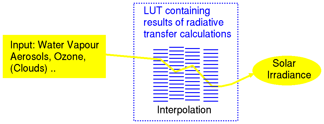
Figure 1The principle of an LUT approach. The transmission is pre-calculated for a variety of atmospheric states with a radiative transfer model (RTM) and saved in a lookup table (LUT). The LUT is then used to determine SSI based on the input given for the atmospheric state for each pixel and time step by interpolation.
Nevertheless, classical LUT approaches still have a significant disadvantage. First, the computation speed is still hampered by the need to interpolate within large multi-dimensional arrays. Second, and more importantly, many RTM calculations must be performed to generate the LUTs, resulting in large and cumbersome binary matrices that raise the recalculation threshold. However recalculation is necessary from time to time to take advantage of new developments. Further, big and cumbersome LUTs increase the chance for hidden bugs. For example, after 4 years of development the CM SAF classical LUTs had a bug, probably induced by a switch in the indices somehow. Thus, 4 years of development were more or less worthless. The LUTs (clear sky, cloudy sky) contained over 100 000 RTM calculations each. As a consequence of the mentioned handicaps and the burden of recalculating classical LUTs, a novel approach was developed, referred to as the “eigenvector hybrid” LUT approach (Mueller et al., 2009). This method takes benefit of the symmetries of atmospheric absorption processes and separates them from the linearly independent processes of aerosol scattering. A further reduction is achieved by the use of the modified Lambert function (Mueller et al., 2004; Ineichen, 2008), which requires only two SZA points (0 and 60∘) to cover the complete SZA dependency in good accuracy. Overall, the number of needed RTM calculations could be scaled down from 100 000 to about 100 without losing accuracy (Mueller et al., 2009, 2012). The RTM calculations were performed with libRadtran (Mayer and Kylling, 2005) using the DISORT solver (Stamnes et al., 1988). The respective retrieval procedure also enables the calculation of direct irradiance, resulting from an adaptation of the Skartveit et al. (1998) model for diffuse irradiance. Overall, this work implements several of the requirements discussed in Pinker et al. (1995) for the improvement of solar surface irradiance retrieval. RTMs are not only needed for the calculation of LUTs but are also essential for the development of parameterisations and a better understanding of the processes in the Earth atmosphere.
2.4 Clear-sky transmittance
The clear-sky irradiance can be derived by multiplication of the extraterrestrial irradiance SSIext with the cosine of the solar zenith angle and the clear-sky transmittance Tclear, according to Eq. (3).
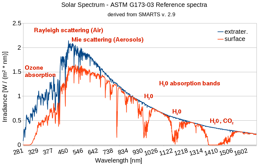
Figure 2Illustration of the solar irradiance spectrum at the top of atmosphere (extraterrestrial irradiance) and the surface for cloud free skies. The main processes leading to the attenuation of irradiance are shown in the associated spectral range.
The term clear-sky radiation is commonly used, but somewhat misleading. It is the radiation received in cloud-free skies, which can still be quite turbid (low visibilities, high aerosol load). The incoming irradiance is scattered and absorbed by gases and particles in the atmosphere. Scattering and absorption lead not only to attenuation of light but also to a modification of the spectra of the extraterrestrial irradiance. Scattering leads to a continuous modification of the spectra, whereas absorption occurs in specific spectral bands, the so-called absorption bands. In these bands the absorption is strong and the radiation is significantly reduced. For example, O3 acts as a strong absorber in the ultraviolet (UV); hence almost all UV-B radiation that enters the atmosphere is absorbed, which is great luck for us, because it causes skin cancer. Further, water vapour has strong absorption bands in the infrared (IR), but also in the microwave, thus acting as a strong greenhouse gas. The absorption bands result from the transition of radiation into periodic vibrations of molecules or atoms (IR) or change in electron state (UV, VIS), whereby the energy of the radiation is used to reach a higher energy level. The effect of the atmospheric scattering is apparent every day. The blue sky results from Rayleigh scattering at air molecules (particles smaller than wavelength λ). The air molecules scatter the incoming irradiance with a wavelength dependency of λ−4. This means that the scattering effect decreases in the power of 4 with increasing wavelength. As a result, blue light is scattered and reflected much more by the sky than other colours, leading to a blue illumination of the sky (blue sky). In contrast, cloud droplets and spherical aerosols follow Mie scattering, which has a wavelength dependency of λ−1 (particles are about the same size as wavelength and assumed to be spheres). Thus there is only a small dependency on the wavelength, leading to grey sky. Scattering forces the light to deviate from the direct path and is induced by the interaction of the photons with the respective media as a consequence of oscillating electric fields or by consideration of the wave–particle dualism of quantum physics as particle-to-particle collisions. More details can be found in Jackson (1998). The great majority of air molecules (N2, O2, noble and inert gases) are well mixed and uniformly distributed and do not affect the spatial and temporal variation in solar surface irradiance. Even the rather small fluctuations of methane and CO2 have no significant effect on SSI variation. Thus, their effect is rather static in space and time, and they pose no problem for the estimation of SSI as a static transmission can be assumed (Müller, 2012). In contrast, ozone, water vapour and tropospheric aerosols are not well mixed. Their distribution is driven by atmospheric dynamics. They show significant temporal and spatial gradients and patterns on different scales. Thus, the spatial and temporal variation in clear-sky irradiance is dominated by these parameters. Yet, the effect of ozone on the broadband solar irradiance is rather small and is therefore neglected in some methods. Sources of information for these variables are discussed in detail in Sect. 7.2. Figure 2 shows the irradiance at the top of the atmosphere and the surface on an inclined plane at 37∘ tilt (toward the Equator) for a US standard atmosphere and aerosol load and a SZA of 48.18∘. The respective data were downloaded from NREL (NREL, 1998), where more details on the atmospheric components are given.
Different methods are applied to consider the effects of the clear-sky components on the solar surface irradiance. A set of models use semi-empirical functions to derive the clear-sky irradiance (e.g. Ineichen and Perez, 2002; Beyer et al., 1996; Cano et al., 1986; Rigollier et al., 2004; Bird and Hulstrom, 1981; Sengupta and Peter, 2003; Perez et al., 2002). More complex methods are based on lookup tables derived from radiative transfer modelling (e.g. Gupta et al., 2001; Mueller et al., 2004, 2009) or some kind of hybrid of the two. However, as a satellite retrieval of SSIclear is not needed for a proper and accurate estimation of SSI (Mueller et al., 2012, 2009, 2004; Müller et al., 2015), the further discussion of the methods focuses on the retrieval of the cloud transmittance.
2.5 Cloud transmission
Overall, clouds are the dominant atmospheric component for the spatial and temporal variation in solar surface irradiance. Thus, accurate information of the cloud transmittance is crucial for the accurate retrieval of solar surface irradiance. Satellites measure the reflection of the surface and atmosphere. In order to derive the cloud transmission, the reflection of the surface and clear-sky atmosphere has to be separated from that of the clouds. The scattering effect of clouds is by far dominant, and absorption can be neglected to a good approximation. Thus, radiation that is not reflected by clouds is transmitted through the clouds. Therefore cloud transmission equal to a good approximation is 1 minus cloud reflection; see Eq. (1).
Here, Tcloud is the cloud transmission and Rcloud the cloud reflection. It is important to mention here that the above equation is valid for fluxes. Satellites, however, observe radiances, i.e. photons reaching the satellite from a specific direction; see Fig. 3 for illustration. The reflection of the Earth's atmosphere is usually not isotropic (equal share of radiation in all directions) but depends on the specific direction and viewing angle. Therefore angular distribution models (ADMs), which result from the bidirectional reflectance distribution function (BRDF), have to be applied to transfer radiances to fluxes (Nicodemus et al., 1977). See Loeb et al. (2005) for further details about BRDF and ADM.
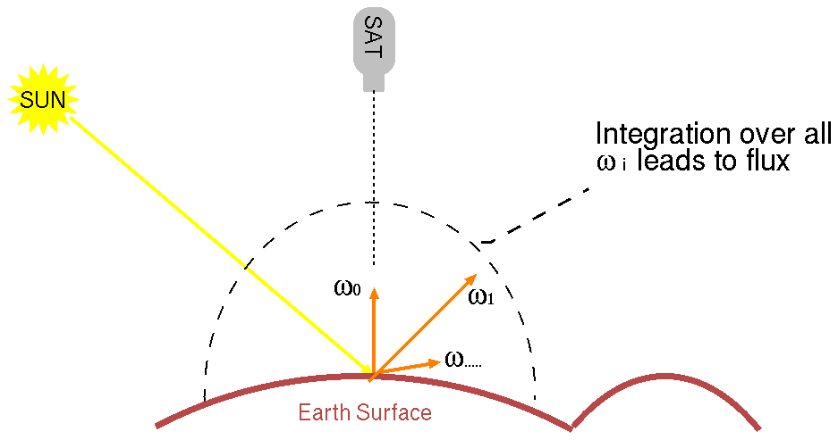
Figure 3Flux is defined as the integration of all radiances over the sphere. The satellite observes the radiance for a specific direction. The reflection of the Earth atmosphere is usually not isotropic (equal amount of radiation in all directions) but depends on the specific direction and viewing angle.
Further, the upward flux depends on the solar zenith angle as the surface albedo (SAL) changes with changing SZA (Briegleb and Ramanathan, 1982). Further, the retrieval of SAL is characterised by severe uncertainties (Shuai et al., 2020; Carrer et al., 2010, 2018; Fell et al., 2021). This adds further difficulties to the accurate definition of ADMs (BRDFs) as the problem is somehow ill-posed. The relation between observed radiances and simulated fluxes depends not only on the viewing geometry but also on land use (e.g. SAL SZA dependency), pixel size, calibration issues (ageing of channels, change of spectral response function) and other effects. BRDF and ADM are also spectrally dependent and hence differ from wavelength band to wavelength band. Thus, they can not be easily transferred from one satellite instrument to another. This poses the question of which path is the best to follow, because there are mainly two different paths to get the cloud transmission. We follow the suggestion of Arvid Skartveit and Jan Asle Olseth (personal communication, 2002) to name them direct and indirect paths. For the indirect path, fluxes and thus ADMs and accurate SAL information are needed. For the direct path this information is not needed but implicitly considered by the satellite observations within the retrieval of the cloud transmission. The two paths are briefly discussed in the following sections.
The cloud transmission can be defined by the micro-physical parameters cloud optical depth (COD) and the effective radii (reff) of cloud droplets. Thus, one way forward is to retrieve cloud optical depth and effective radii, following an approach discussed in Nakajima and King (1990). Once COD and reff are retrieved, the cloud transmission can then be calculated based on RTM parameterisation or by RTM-based lookup tables (LUTs). For example, Deneke and Feijt (2008) use information of cloud physical properties retrieved with a LUT approach for the estimation of surface solar irradiance. The respective retrieval of COD and reff was developed by the Royal Netherlands Meteorological Institute (KNMI) and is applied to retrieve cloud optical thickness, liquid water path and particle size from satellite imagers within the CM-SAF framework (Roebeling et al., 2005). A similar approach was used by ISCCP (Rossow and Zhang, 1995; Zhang et al., 1995) for the generation of CDRs. As mentioned in the method section, several approaches for the retrieval of solar surface irradiance use the cloud optical depth and the effective radii for the estimation of the cloud transmission. However, for the retrieval of COD and reff, accurate surface albedo (surface reflection) and ADM and BRDF simulations are needed in order to separate the reflection by clouds from that of the surface and to transfer radiances to fluxes. Further, the clouds are usually assumed to be plane-parallel, which is a rough assumption. Finally, the problem is somehow ill-posed as the retrieval of COD depends on reff and vice versa and on the ratio between ice and water particles in mixed phase clouds; see Nakajima and King (1990) for details. However this ratio is usually unknown. For some of these effects a quantitative analysis is given by Kato et al. (2006).
Another indirect approach takes advantage of the linear relation between transmission (T) and the top-of-atmosphere (TOA) albedo, as discussed in Li et al. (1993). For a given surface albedo and clear-sky state the cloud transmission changes linearly with increasing COD. Thus, assuming a standard plane-parallel cloud, the relation between transmission and TOA albedo can be pre-computed for a variety of CODs, surface albedos and clear-sky parameters. The precomputed RTM results are saved in a lookup table (LUT). The observed TOA albedo is then used as a variable to retrieve the cloud transmission by interpolation within the LUT. This approach has been the basis for the first operational version referred to as the prototype of the CM-SAF scheme, described and validated in Mueller et al. (2009) and Hollmann et al. (2006). This prototype followed the concepts and ideas of Pinker and Laszlo (1992) and Pinker et al. (1995). Also, the OSI SAF retrieval procedure for SSI uses TOA albedo as input (Marsouin, 2019; Gautier et al., 1980). However, also in this approach clouds are assumed to be plane-parallel, ADMs and BRDFs are needed to convert radiances to fluxes and accurate SAL data are necessary.
In brief, using the indirect approach means to be further away from the observations, as additional assumptions and simulations are needed in contrast to the direct path, which is discussed in the next section.
For the indirect paths (flux-based methods), accurate SAL and ADMs and BRDFs are needed. Further the clouds are assumed to be plane-parallel. These induce uncertainties in the estimation of the cloud transmission and motivate the use of the direct path. The direct path relates the measured reflection (radiances) directly to the cloud transmission without the need of any radiative transfer modelling, ADM or SAL, as they are implicitly considered by observations. In the following the method applied at CM SAF and DWD is described in more detail. It is based on the concepts of Möser (1983), Möser and Raschke (1984), Cano et al. (1986), and Diekmann et al. (1988) and originates from the Heliosat code developed at the University of Oldenburg (Beyer et al., 1996; Hammer, 2000; Hammer et al., 2003). Only observed radiances are needed in order to retrieve the effective cloud albedo (Mueller et al., 2011), which is also referred to as cloud index or effective cloud coverage. The effective cloud albedo (CAL) is defined as the normalised relation between the all-sky and clear-sky reflection derived from satellite images in the solar spectral range. CAL is linearly related to the cloud transmission for CAL values lower than 0.8. A clear-sky model is used afterwards to calculate the solar surface irradiance based on the retrieved cloud transmission according to Eq. (2). This approach is still the basis for several state-of-the-art retrieval schemes, described in more detail in Dürr and Zelenka (2009), Posselt et al. (2011b), Mueller et al. (2012), Müller et al. (2015), Castelli et al. (2014), and Pfeifroth et al. (2019b).
In order to derive the effective cloud albedo, it is important to consider the effect of the solar zenith angle on the extraterrestrial irradiance. Furthermore, the dark offset of the instrument has to be subtracted from the observed reflections. Thus, the observed reflections are normalised by application of Eq. (6) in a first processing step.
Here, D is the observed digital count (including the dark offset). D0 is the dark offset, the instrument's value in the dark, which is provided by EUMETSAT. The Sun–Earth distance variation is considered by the factor f. Finally, the cosine of the solar zenith angle corrects the different illumination conditions at the top of the atmosphere introduced by different solar altitudes. The resulting ρ is referred to as normalised reflection. The effective cloud albedo is then derived from the normalised reflection ρ, the clear-sky reflection ρcs and the calibration value ρcal by Eq. (7).
Here, ρ is the observed normalised reflection for each pixel and time. ρcs is the clear-sky reflection, which is derived for every pixel and time slot separately. In principle this is done by applying statistics over the lowest reflections observed during a typical time span of 3–4 weeks, e.g the average of the lowest reflections within an epsilon band, which can be defined by the user and is typically about 10 % of ρcal. Also, percentile functions can be used, but based on tests at DWD this is expected to lead to a lower performance. Further details on the method to derive ρcs are given in Hammer (2000), Müller et al. (2015), and Mueller and Trentmann (2015). The need to calculate ρcs for every time slot of the day results from the strong dependency of the clear-sky albedo (which is in turn usually dominated by the surface albedo) on the solar zenith angle (Briegleb and Ramanathan, 1982). ρcal is a measure for the reflections observed for the highest cloud albedos. It is therefore often also referred to as the “maximum” reflection ρmax. It is typically determined by the 95th–98th percentile of all reflection values at local noon in a target region, characterised by high frequency of cloud occurrence for each month (Mueller et al., 2012; Müller et al., 2015). In this manner changes in the reflections induced by the satellite are accounted for (Posselt et al., 2011a). Further, it also calibrates the reflections between clear sky (CAL = 0) and “maximum” overcast (CAL = 1).
For CAL values below 0.8, the relation between CAL and Tcloud is simply given by
Thus,
For very thick clouds SSI does not decrease linearly any more with CAL as a result of lateral scattered light, and a modification of the relation (9) is needed, e.g. as follows.
The term Heliosat is widely used in the energy meteorology community for methods using the relation given in Eq. (7). Yet, this naming is somehow misleading. In some Heliosat methods the observational approach for ρcs is partly replaced, e.g Heliosat-2 (Rigollier et al., 2004), or completely replaced, e.g. Heliosat-5 (Tournadre et al., 2021), by modelling of ρcs. However, the planetary reflection is in good approximation observed by the satellite, and a separation of the effect of ground albedo and atmospheric reflection or a complete replacement of ρcs with RTM simulations is a detour adding additional uncertainties. The motivation for these modifications is incomprehensible both from the point of view of measurement technology and from the point of view of radiative transfer modelling (see Sect. 3 and the open reviewer comments; Tournadre et al., 2021). In order to avoid misunderstandings, we introduce the term CALSAT for the described method and use it instead of Heliosat throughout the paper. The CALSAT approach has been applied routinely in real time at the University of Oldenburg since 1995. It was used to establish the server Satel-Light, which delivers valuable information on daylight in buildings to architects and other stakeholders (Fontoynont et al., 1997). The method was also used to provide the data for successful projects like PVSAT and PVSAT-2 (Lorenz et al., 2004; Hammer et al., 2003), which went into 24/7 operational services. All CM SAF Climate Data Records (CDRs) (Posselt et al., 2011b; Müller et al., 2015; Pfeifroth et al., 2019b) have been retrieved with the CALSAT approach coupled with a clear-sky model based on the eigenvector hybrid LUT method (Mueller et al., 2009). The respective data sets belong to the most used and validated data sets in the world covering a wide field of applications, as can be seen from recent publications (Wild et al., 2021; Kulesza, 2021; Alexandri et al., 2021; Gardner et al., 2021b, a; Farahat et al., 2021; Yang and Gueymard, 2021; Kulesza and Bojanowski, 2021; Fountoulakis et al., 2021; Drücke et al., 2021; Daggash and MacDowell, 2021). CAL-based SSI data are characterised by a high accuracy and homogeneity, which is a reason for the popularity, even up to quality control of ground-based stations (Urraca et al., 2017, 2020). The CM SAF SSI data are regularly validated by the CM SAF team, e.g. Pfeifroth et al. (2019a), but also by the user community (e.g. Wang et al., 2018; Amillo et al., 2018; Urraca et al., 2007; Trolliet et al., 2018; Riihelä et al., 2015; Posselt et al., 2011b; Ineichen et al., 2009, and references therein). The complete list of peer-reviewed articles dealing with CM SAF radiation data is available on http://cmsaf.eu (last access: 14 March 2022) under the menu item Publications (CMSAFpubl, 2021). Even if only the CM SAF data are counted, there are already thousands of users all over the world (Selbach and Thies, 2021). There are of course much more if the other data providers are accounted for. All CM SAF validation reports, product user manuals, algorithm theoretical baseline documents and operations reports are available on http://cmsaf.eu under the menu item Documentation. The CAL-based CM SAF SSI data also went into the PVGIS service (Huld et al., 2012; Amillo et al., 2014), which has several hundreds of accesses per week (Thomas Huld, personal communication, 2012). Finally, the CALSAT method is also used at DWD to generate 24/7 operational near-real-time data and forecasts, which are available at DWD (2022). In summary, the direct approach using the observable CAL to define the cloud transmission is quite well established and is used for the creation of radiation data sets that are widely used around the world, e.g. Selbach and Thies (2021). It enables the retrieval of monthly means with an accuracy of 5.2 and 7.7 W m−2 for SSI and direct irradiance, respectively (Pfeifroth et al., 2019a). Hereby, the mean absolute difference is used as a metric for the accuracy. It is defined as the average of the absolute values of the differences between the ground-based measurements and the satellite-based irradiance first over all months and then over all stations. For the validation all available BSRN stations were used.
The uncertainty in CALSAT SSI trends is quite small, with W m−2 per decade, which shows the adequate homogeneity of the data set and its ability to identify climate trends and decadal variability.
Already the early CALSAT methods had a significant impact. For example, the method developed by Möser and Raschke (1984) and Diekmann et al. (1988) was routinely applied at the German Weather Service till it was replaced by a modified SPECMAGIC (Mueller et al., 2012) version in 2018. A similar method was also used for the GEWEX Surface Radiation Budget Project as a quality control algorithm (Gupta et al., 2001; Darnell et al., 1992). This algorithm known as the Staylor algorithm was chosen by the World Climate Research Program (WCRP) SRB project for generation of surface solar irradiance for a test period of several years (Whitlock et al., 1995) and has been used to produce a long-term data set. Finally, the CALSAT approach has also been adapted to polar-orbiting satellites as effective cloud fraction (Wang et al., 2014, 2011).
The demand for spectrally resolved irradiance has increased significantly in recent years due to new solar cell technologies and increased awareness of climate change. The importance of the spectrally resolved irradiance (SRI) for the efficient planning of PV systems is discussed in Huld and Amillo (2015). Further, SRI is of benefit for a more extensive monitoring and analysis of the climate system and enables the generation of essential meteorological variables for several application fields, e.g.
-
daylight, which is of importance for the design and planning of office buildings and health studies, e.g. concerning seasonal affective disorder;
-
ultraviolet (UV)-A and UV-B, important for weather warnings concerning UV dose; and
-
photosynthetic active radiation (PAR), important for agro-meteorology.
However, retrieval algorithms for the generation of accurate long-term series of spectrally resolved irradiance covering the complete solar spectrum were not available or applied to generate CDRs until 2012. The development of SPECMAGIC (Mueller et al., 2012), a fast and accurate method for the retrieval of spectrally resolved irradiance, was a game changer. It has been used to improve the quality of the broadband radiation of the CM SAF CDRs but also to provide the first spectrally resolved solar irradiance climate data record.
The SPECMAGIC method is an adaptation of the concept for the broadband radiation (Mueller et al., 2009) to Kato bands (Kato et al., 1999) using the correlated-k approach offered as part of libRadtran (Mayer and Kylling, 2005). The correlated-k method is developed to compute the spectral transmittance (hence the spectral fluxes) based on grouping of gaseous absorption coefficients. However, in contrast to Mueller et al. (2009) the cloud transmission is derived with the CAL approach in SPECMAGIC (Mueller et al., 2012), and only the clear-sky irradiance is calculated with an eigenvector LUT. The CALSAT method was developed for broadband radiation. Thus, a spectral correction of the broadband transmission was needed, which was done by a RTM-based spectral correction factor for the broadband CAL. A detailed description of the methods is given in Mueller et al. (2012). Further validations were presented in Amillo et al. (2015). As ground measurements of spectrally resolved irradiance are extremely rare, satellite-derived information constitutes the primary data source for spectrally resolved irradiance within the scope of climate monitoring and solar energy applications. The validation of the spectrally resolved irradiance climate data record (SRI) in Ispra (Italy) shows an accuracy of the monthly mean values of spectrally resolved data higher than 0.03 W m−2 nm−1 for wavelengths below 1000 nm and even better for longer wavelengths (Pfeifroth et al., 2019a).
Over recent decades the share of solar energy has increased enormously around the world, as already briefly discussed in Sect. 1. In contrast to fossil and atomic energy, solar resources are fluctuating and the energy yield depends on the weather. Variations in solar radiation, and thus in solar energy, have to be balanced, by either increase or decrease in the production from conventional power plants or by trading energy on the electricity market. The shorter the time for this compensation, the higher the costs and the lower the efficiency of renewables. In addition, wrong forecasts of extreme weather events might also lead to grid instabilities and regional overloads. Accurate forecasts are therefore needed to enable an efficient planning and operation of the energy production and to optimise the use of renewable energies and the reduction of CO2 emissions. Besides forecasts, instantaneous near-real-time data are also essential for the optimisations and monitoring of solar energy systems. As a result, the demand for accurate near-real-time data and forecasts of solar surface irradiance has steadily increased. Satellite-based cloud information is well suited for the estimation of near-real-time radiation data and the basis for short-term forecasts, which outperform NWP in the first hours (Lorenz et al., 2017; Urbich et al., 2019). However, forecasting SSI is not only needed within the scope of solar energy but is also useful for weather warnings concerning UV radiation, heat waves, droughts and evaporation.
The satellite-based short-term forecast of SSI, also referred to as nowcasting, is usually done by retrieval of atmospheric motion vectors from satellite images and subsequent application to extrapolate the observed clouds into the future. The predicted cloudiness can then be used to calculate SSI with one of the methods discussed in Sect. 4. In order to get the forecasts in the needed spatial and temporal resolution, a dense field of cloud motion vectors is needed. The use of cloud motion vectors for nowcasting is widespread, and many approaches have been proposed so far; for example Gallucci et al. (2018) and Sirch et al. (2017) used cloud motion vectors from SEVIRI (Spinning Enhanced Visible and Infrared Imager) on board Meteosat Second Generation (MSG) to forecast solar surface radiation for up to 2 h. Further methods to gain AMVs are discussed for example in Raza et al. (2016), Wolff et al. (2016), Antonanzas et al. (2016) and Barbieri et al. (2017). In recent years, however, computer vision techniques (Szeliski, 2011) have found their way into meteorology and have offered the advantage of a strong developer community, which is typical for open software. This led to the use of optical flow methods for the estimation of atmospheric motion vectors. Optical flow has been used pre-dominantly for image pattern recognition in the fields of traffic, locomotion and face recognition (Sonka et al., 2014). To our knowledge, one of the first applications in meteorology has been the utilisation of the optical flow for radar images as described by Peura and Hohti (2004). At DWD the TV-L1 method (Zach et al., 2007) was implemented in 2018 for the short-term forecast of radar reflectivity by Manuell Werner. This has motivated the adaptation of TV-L1 to CAL images (Urbich et al., 2018) in order to track the cloud movements and to extrapolate the CAL values with optical flow. In order to meet the requirements of the operational near-real-time retrieval of CAL, SPECMAGIC (Mueller et al., 2012) has been modified. The modified version is referred to as SPECMAGIC_NOW. The visible channel in the 600 nm band is used instead of the broadband visible channel, which is gained from a combination of VIS006 and VIS008 (Cros et al., 2006). Further, running backward statistics are performed to calculate ρcs. In contrast to SPECMAGIC, only 20 d are used for the statistics. Also, the estimation of ρcal has been modified. Please see Sect. 7 for further details.
The combination of the effective cloud albedo with TV-L 1 and SPECMAGIC_NOW delivers a novel powerful method for the short-term forecast of solar surface irradiance, as discussed in Urbich et al. (2019). Yet, for the satellite-based nowcasting, two subsequent images are needed. Before sunrise no former image in the visible is available for the estimation of the atmospheric motion vectors. Thus, the University of Oldenburg extended the Heliosat method to infrared images (Hammer et al., 2015). For longer forecast horizons a blending with NWP models is needed (Urbich et al., 2020; Lorenz et al., 2017). However, cloud motion vector methods have the disadvantage that they can not capture convection or dissipation (change in intensity). Although NWP also has great difficulties in this area, they include at least physical parameterisations to deal with the phenomena. That is the reason why after a couple of hours NWP models outperform nowcasting (NWC), and a combination of both methods is needed in order to gain the optimal accuracy for every time step. The near-real-time data and forecasts up to +18 h are available at the DWD open data server (DWD, 2022).
7.1 Method
A central paradigm of science is the goal to make things as simple as possible and as complex as necessary and to benefit from the knowledge gained. In this context, we would like to briefly review the lessons learned within the Heliosat-3 project. The goal of the Heliosat-3 project (Betcke et al., 2006) was to supply high-quality solar radiation data gained from the exploitation of existing Earth observation technologies by taking advantage of the enhanced capabilities of the new Meteosat Second Generation Satellites. Therefore one aim was to develop a method to replace the CALSAT method by a method using cloud micro-physical parameters. During the Heliosat-3 project, the meteorologists Skartveit and Olseth reminded us not to forget the advantages of the direct path, using CAL derived from satellite measurements. Lessons learned within Heliosat-3, CAL is still used and was not replaced by an approach using COD and reff at the University of Oldenburg, the leading entity of the project. Further, within CM SAF the LUT approach used in the early phase for the generation of the first data sets (Mueller et al., 2009) has been replaced by the CALSAT approach concerning cloud transmission for the generation of CDRs (Posselt et al., 2011b; Müller et al., 2015) and the generation of near-real-time data and forecasts (Urbich et al., 2018). For clear-sky cases RTM-based LUTs are still used in the CALSAT approach, besides other arguments, in order to overcome the limitation of turbidity as input (Mueller et al., 2004).
Thus, the CALSAT approach has not been replaced by flux-based methods at leading institutes and is to the knowledge of the authors still the best way forward for the retrieval of cloud transmission. The approach results from the law of energy conservation and relates the observed reflection directly to the effective cloud albedo and the cloud transmission without the need for external SAL data or ADM simulations. In these terms the CALSAT method takes full advantage of the satellite measurements in the visible (Mueller et al., 2011). The data sets of the University of Oldenburg, CM SAF and other entities using CAL are among the most validated data sets of the world. The validation results around the SAF radiation data show that the improved CALSAT methods are in the meanwhile able to derive accurate SSI data close to the accuracy of well-maintained ground-based stations (Posselt et al., 2011b; Müller et al., 2015; Pfeifroth et al., 2019a). The high quality of CAL-based SSI data even enables the monitoring of ground-based measurements (Urraca et al., 2017, 2020) and the use for climate trend analysis (Pfeifroth et al., 2018). The success and impact of the CALSAT approach is impressive. Nevertheless, further improvements of CALSAT have been performed and are still under progress. Yet, many of these improvements are not CALSAT specific but represent general issues of satellite-based retrieval of SSI. The following sections provide a discussion of limitations and possible improvements of these retrievals to the best knowledge of the authors.
7.1.1 Mountains
The pixels of the visible MSG full disc channels (VIS006 and VIS008) are relative large over the European mountains, with a size of 3–5 km. This leads to pixels which cover mountains and valleys and are therefore no longer spatially representative of the area covered. The terrain is too heterogeneous, and the spatial representativeness is largely limited by the resolution of the VIS006 and VIS008 channels. However, over Europe and large parts of Africa the high-resolution visible (HRV) channel is available. It has a sub-satellite resolution of 1 km × 1 km, which means about 1 km × 2 km over the European mountains. The spatial representativeness is significantly improved by the higher spatial resolution and is a central key for the improvement of the precision and accuracy of SSI in mountainous regions (Dürr et al., 2010; Dürr and Zelenka, 2009).
Deep valleys are shadowed by mountains, reducing the amount of available solar surface radiation. The shadowing information needs to be corrected by the use of additional geographical information and geometrical functions. For this correction, the location, size and height of the mountains are needed, which are provided by a digital elevation model (DEM). Respective data are available free of charge from various web sites; see OpenDEM (2022). Geometric functions can be used to calculate the solar zenith angle and azimuth angle for every date and hour, enabling correction of the shadowing based on the DEM information. This correction is independent of the retrieval method for SSI. A respective correction as well as further mountain-specific features has been implemented into the CALSAT approach by Dürr and Zelenka (2009). The work of Dürr and Zelenka (2009) has been the basis for the HelioMont algorithm (Stöckli, 2013; Castelli et al., 2014), which comes with further improvements.
Further, snow-covered surfaces occur with much higher frequency in mountains than in lowlands. Thus, the treatment of clouds over snow also needs more attention in the mountains. Dürr and Zelenka (2009) implemented a correction for the CAL retrieval over snow and demonstrated that it leads to higher accuracy.
7.1.2 Long-lasting clouds
All methods need cloud-free pixels in order to get actual information of the surface albedo (indirect flux-based methods) or the clear-sky reflection ρcs. Outdated information of SAL or clear-sky reflection can lead to significant errors in SSI. The clear-sky reflection and the surface albedo can only be derived from satellites in cloud-free situations. Thus, long-lasting clouds are a serious error source for the satellite-based retrieval of SSI. This is valid for all retrieval methods. Long-lasting clouds can contaminate the observation of ρcs. The minimisation of ρcs leads only to the clear-sky reflection if at least one pixel during a certain time interval is cloud free. However, especially in winter at higher latitudes (e.g. northwestern Europe), it can happen that there is no cloudless sky for 20–30 d, which leads to cloud contamination and an overestimation of ρcs and, in turn, to an underestimation of CAL.
An option to reduce the uncertainties induced by long-lasting clouds might be the use of simulated ρcs based on RTMs or climatological values for ρcs as a backup. The former option has been implemented in SPECMAGIC_NOW, a SPECMAGIC modification dedicated and used for the 24/7 production of near-real-time data at DWD. However, the method for the decision when the backup is used is still in development and needs further evaluation. Another option is to fit the diurnal variation in ρcs and to replace outliers by the fitting function; see HelioMont for details (Castelli et al., 2014). This approach requires clear skies for adjacent time windows and can therefore only mitigate, not solve, the problem of long-lasting clouds. However, it must also be considered that long-lasting clouds typically occur during wintertime at higher latitudes and are therefore associated with low absolute SSI values and hence also low absolute errors. Even with a backup for ρcs, CAL would still be derived directly from observations for the vast majority of cases.
7.1.3 Improvement of clear-sky reflection, ρcs method
Usually the broadband visible channels are used for the CALSAT method, either directly or as a combination of the visible channels in the spectral bands 600 nm (VIS006) and 800 nm (VIS008) according to Cros et al. (2006). However, the precision of the ρcs detection might be improved by using the VIS006 channel as the reflection in this band is rather dark for vegetation. This enhances the contrast between clear-sky and cloudy reflection and enables a higher precision for optical thin clouds. A comparison of using different VIS channels was performed by Posselt et al. (2011a). This study showed the potential of using the VIS006 channel and motivated its use for SPECMAGIC_NOW. Experiments to improve the accuracy by using percentiles instead of the original statistical method (Hammer, 2000) did not lead to an improvement. Hence, the same method is used for the calculation of ρcs in SPECMACIC (Mueller et al., 2012) and SPECMAGIC_NOW.
Misclassification of snow-covered surfaces as clouds or vice versa is a serious error source for all methods. This is also valid for the CALSAT method, but with some specificity resulting from the ρcs method. To illustrate, let there be a certain number of snow-free and snow-covered days within the 20–30 d period used for the retrieval of ρcs. As ρcs is calculated with a minimisation function, ρcs will always capture the snow-free situation. For the snow-covered days the snow will be treated as a thick cloud resulting in a large underestimation of SSI. This effect can be reduced if ρcs is calculated with a fuzzy logic approach, discussed in detail in Posselt et al. (2011b). However, as experienced by the CM SAF the Fuzzy logic approach induced other artefacts, e.g. wrong ρcs values in the desert. There might be another option to treat this problem. An accurate snow map can be used to flag snow-covered regions and to correct ρcs by simulated values if ρcs shows too low values for snow. Of course this approach would be a rough workaround which needs further optimisation and adjustments based on validation studies. A worldwide reference for snow cover maps is provided by NIC NOAA, referred to as the IMS snow ice map (Helfrich et al., 2018). This map is based on several satellite instruments including microwave as well as ground-based information and is therefore not so prone to long-lasting clouds. However, melting periods of snow are still sometimes not captured by IMS as a result of long-lasting clouds as discussed in the snow workshop (Helmert et al., 2018).
The upcoming CM SAF SARAH-3 data record is based on internal snow detection with the aim of better detecting snow-covered surfaces. The method is based on optical flow, assuming that cloud objects move much faster than snow objects, allowing separation of clouds and snow. Initial results indicate significant improvements, but the validation is still in progress. A detailed discussion of this approach and its validation will be included in the SARAH-3 documents. A comprehensive discussion of this approach and its validation will take place in the SARAH-3 documents.
In SPECMAGIC_NOW the duration used for the slot-wise detection of ρcs has been reduced from 30 to 20 d. This is expected to reduce the effect of snow misclassification as cloud but might be a handicap for long-lasting clouds. However, for Germany the operational comparison with other data sets (DWD in situ network, SPECMAGIC) have not shown any significant drawbacks concerning long-lasting clouds so far.
7.1.4 Calibration
An accurate calibration is of very high importance for the generation of homogeneous climate data records. Thus, it is the basis to enable appropriate trend analysis. The focus of the first geostationary Meteosat satellites was the support of weather monitoring and forecasting. As a result calibration issues of the visible channels were not considered (thoroughly) for MVIRI on board MFG and for SEVIRI on board MSG. Both instrument generations are not equipped with onboard calibration units for the visible channels. The increased awareness of climate change and the need for improved climate monitoring and analysis has also led to the demand to use Meteosat satellite data for climate monitoring. As a result, CM SAF was implemented by EUMETSAT in 1999 and the activities concerning calibration of the visible channels increased. For example, Govaerts et al. (2004) developed a method for the calibration of the SEVIRI visible channels using desert and cloud targets as radiation references. However, longer time series are required for a CDR, which requires the use of MVIRI to extend the time series, but the method of Govaerts et al. (2004) is not applicable to MVIRI. Unfortunately the MVIRI time series is quite inhomogeneous as in the early days of MFG changes in the gauge were not unusual. Further, up to Meteosat-6 no inter-calibration between the satellite instruments was done, adding additional breaks in the observed reflections; see Fig. 4.
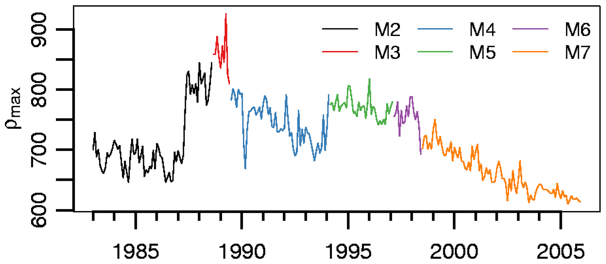
Figure 4Temporal evolution of the 95th percentile (ρmax) of the observed reflections for MVIRI, covering 1983 to 2005. The different MVIRI instruments (M2–M7) are coloured for a better distinction. Image from Posselt et al. (2011a).
For these reasons CM SAF took advantage of the calibration value ρcal of the CALSAT method (see Eq. 7) for the self-calibration of Meteosat instruments (e.g. MVIRI and SEVIRI). This is described in more detail in Posselt et al. (2011a). Basically, the ρ values are ordered with a function in a first step. Then the 95th or 98th percentile is used as ρcal. This is done for a target region with a high cloud coverage (Atlantic Ocean, southwest of southern Africa). The advantage of this approach is that the calibration is done for the same targets (clouds) for which the transmission is retrieved. It has been shown that the method leads to stable homogeneous data sets across satellite generations (Posselt et al., 2011b; Pfeifroth et al., 2018).
This approach has been slightly modified for SPECMAGIC_NOW. First of all another target region is used, following an approach of the Royal Meteorological Institute of Belgium (RMIB). The novel target region covers the intertropical convergence zone (ITC) region. It is defined from line 1234 to 2486 of the Meteosat level 1.5 images. Here all counts of the 12:00 UTC slots are sampled over a period of 3 d and sorted with the heapsort function and subsequently assigned to a vector (fper). Then, the indices of percentile 95 (pm) and percentile 99.99 (pmm) are calculated. Afterwards, ρcal is calculated within a loop between the indices of the respective radiances and finally multiplied by 1.1. Please see the C-code lines in the Appendix for details.
Comparison with the former method of CM SAF for the calculation of ρcal indicates that this method leads to less noise. As SPECMAGIC_NOW is operated 24/7 using SEVIRI as input, the method of Govaerts et al. (2004) could be applied. However, concerning physics, the ρcal method described above has a significant advantage. Identical channels and targets (clouds) are used for both the calibration and the retrieval of CAL. Yet, the Govaerts et al. (2004) method uses desert targets in addition, which is expected to add uncertainties to the calibration because the spectral albedo is quite different to that of clouds. At least during the development and testing of SPECMAGIC the ρmax calculation could not be improved by the use of additional desert targets.
7.1.5 Parallax correction
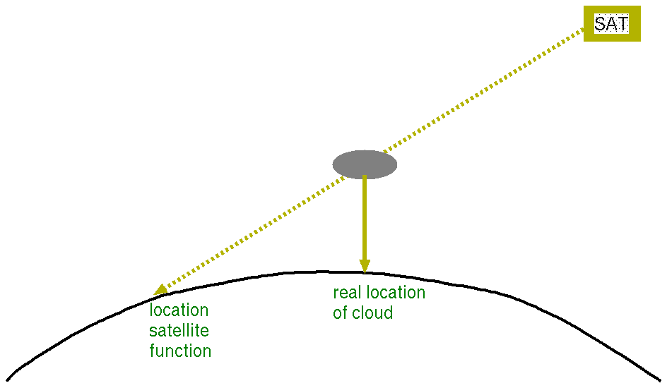
The geolocation of the satellite is always related to the Earth surface (sea level). This means that independent of cloud height the cloud is assumed to be at the surface. The higher the clouds and latitudes, the larger the displacement of the geolocation. For example, for a cloud with a top height of about 10 km the displacement effect at midlatitudes is several kilometres. This hampers the comparison between satellite data and ground-based information, in particular if instantaneous data and not averages are compared. The parallax effect is illustrated in Fig. 5. EUMETSAT offers a geometrical function for the correction of parallax effect, which needs only latitude, longitude and the cloud top height (CTH) as input. The CTH can be estimated from the brightness temperature of the window channel at 10.8 nm. The displacement is then calculated based on geometrical (sin cos) functions. This approach works well for the infrared channels. In the IR the satellite receives mainly the emission from the cloud top if the clouds are not semi-transparent, which can be assumed for a COD larger than 10. Thus, CTH can be used for the needed altitude information for the parallax correction. However, the diffuse part of SSI is reflected throughout the cloud, and the height needed for the parallax correction can not be assumed to be close to the top of the cloud. Therefore, the parallax correction should only applied to the direct radiation. The application of a parallax correction for direct irradiance was already postulated in 1996 by Beyer et al. (1996). A parallax correction has been implemented in the HelioMont method (Stöckli, 2013; Castelli et al., 2014), but the reduction in the error measures was marginal compared to other more dominant effects (Reto Stöckli, personal communication, 2021). One reason might be that for COD larger than about 10 direct irradiance is zero. This means that diffuse radiation usually dominates SSI in cloudy situations, and CTH is not well suited for the correction. Thus, the optimal definition of the cloud height for the parallax correction needs further investigations, in particular empirical studies and RTM calculations for different cloud scenes, especially since the parallax correction could be more significant in homogeneous terrain. After all, the parallax effect is not a weakness of a specific retrieval method but results from the viewing geometry. Close to the Equator, everything is fine.
7.1.6 Slant column correction
The geostationary orbit leads to slant column viewing geometries at higher latitudes and towards the western and eastern borders of the satellite field of view. As a consequence the “cross section” of the clouds increases significantly; see Fig. 6 for illustration. Thus, on average the cloud coverage is artificially enhanced at larger satellite zenith angles, leading to an underestimation of surface solar radiation. The validation study of Riihelä et al. (2015) provided a clear indication for the underestimation with increasing latitude. Based on these results, a brief empirical correction has been developed and implemented in SPECMAGIC for the generation of the SARAH 2.1 data set (Pfeifroth et al., 2019c). The correction term for the slant geometry effect is approximated as a function of the satellite zenith angle θsat:
The correction term is afterwards applied for and CAL>0.04.
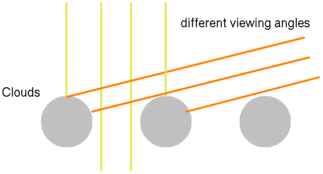
Figure 6Illustration of the slant geometry effect. For a satellite zenith angle of 0 the cloud coverage would be 0.5, but for the slant geometry it would be 1.
This results in an improved performance of the retrieval, especially in higher latitudes (Pfeifroth et al., 2019a). Yet, further empirical studies and RTM calculations are needed to improve the correction of the slant geometry effect. Again this effect is relevant for all methods. The cloud cross section also increases with increasing SZA, but here the reflection also increases as cloud optical thickness is increasing, but the slant viewing geometry of the satellite leads to an artificially increased cloud cover that does not match the ground observations.
7.1.7 Deep learning – neural networks
Overall, the use of artificial intelligence methods, in particular deep learning (machine learning) with neural networks (NNs), is also increasing in meteorology. This also includes the estimation of solar surface irradiance from satellites (Senkal, 2009; Yeom et al., 2019; Cornejo-Bueno et al., 2019; Dewitte et al., 2021).
However, a drawback of neural networks is their black box character and the need for retraining for new regions and satellite systems. A neural network is, strictly speaking, only valid for the training framework, as only the behaviour of the training data sets can be reproduced. An application to other regions, periods or satellite instruments typically requires extensive re-training. That is a reason why scientists started to develop spectral transfer functions to ease the adaption of the network to other satellite instruments. However, this means using physical approaches to avoid the need for extensive retraining. Further, the black box character hampers a deeper understanding of the involved physics and consequently the analysis of error sources. Ultimately, it is a complex regression, and the term intelligence is somehow misleading. For the retrieval of solar surface irradiance the physics is well defined. Thus, it is not obvious what advantage NN could provide compared to physical approaches. However, a good application of neural networks (NN) might be the replacement of LUTs. This has been done for the retrieval of SIS (e.g. Takenaka et al., 2011). In this study an algorithm for estimating solar radiation from space using a neural network (NN) to approximate radiative transfer calculations was developed. Similar approaches are also used for other atmospheric variables, e.g. for volcanic ash (Bugliaro et al., 2021). However, with respect to SSI, the burden of cumbersome LUTs, which require hundreds of thousands of RTM calculations, is eliminated by using the hybrid eigenvector LUT concept (Mueller et al., 2009). These LUTs are relatively easy to calculate and to manage. This might reduce the value of NNs as a replacement of LUTs within the scope of SSI. Thus, the authors believe that there is no urgent need to apply neural networks for the retrieval of solar surface radiation, in particular if the CAL approach is used for the retrieval of the cloud transmission.
7.2 The clear-sky input data
Three SAFs are engaged in the retrieval of SSI. EUMETSAT triggered an intensive discussion and interaction between the SAFs in order to exploit synergies. As a consequence, a comparison of the SAF SSI data (Ineichen et al., 2009) was done, and several SAF radiation workshops took place. It was discussed that all SAFs use established methods for the retrieval of the cloud transmission but that there is a need for action on the clear-sky input data. Therefore, the clear-sky input data are briefly discussed in the following paragraphs.
7.2.1 Ozone
O3 is a strong absorber and can be well detected from satellites. Data in good quality can be gained from GOME/SCIAMACHY (Burrows and Chance, 1992), TOMS (Fleig et al., 1986) and the Ozone Measuring Instrument (Ziemke et al., 2011) and the respective follow-up satellites. There is no need to use data in high temporal resolution as the spatial and temporal variation in SSI is dominated by clouds at the mesoscale. Thus, observations based on polar-orbiting satellites are not a handicap. Alternatively ozone data from the ECMWF models can be used (Bechtold et al., 2008). However, climatologies can also be used in good approximation for broadband SSI as a deviation of about 150 DU from the US standard atmosphere leads only to changes in SSI of about ±5.5 W m−2. This is in the range of the uncertainty of solar irradiance measurements (Müller, 2012). However, the absorption effect of ozone in the UV is very strong, and therefore accurate information about the ozone concentration is required for this spectral range.
7.2.2 Water vapour
Water vapour (H2Og) is a strong absorber, and the total column can be well retrieved from satellites. However, H2Og can only be retrieved in cloud-free skies without appropriate profile information. Thus, using H2Og from satellite is expected to induce a clear-sky bias in H2Og. Therefore, data from NWP might be the better option as the water vapour channels are assimilated by modern state-of-the-art NWP models (4D-Var). Thus, this data source is strongly recommended for H2Og; e.g. CM SAF is using water vapour information from the ECMWF NWP model and from the ERA-5 reanalysis (Dee and Uppala, 2009; Betts et al., 2003). Also OSI SAF uses data from ECMWF. The use of climatologies can lead to significant deviations for daily and hourly SSI (broadband) values and is not recommended as a primary choice.
7.2.3 Surface albedo
Satellites are a good source for gridded surface albedo (SAL) data. The optimum accuracy for the retrieval of SAL is about 5 % (Fell et al., 2021; Riihelä and Kallio-Myers, 2020). The accuracy is limited by uncertainties in ADMs, spectral response functions and calibration of the visible channels. This could lead to different SAL values for different instruments. For example, during the CM SAF CDOP-1 phase the SAL values derived from MSG and NOAA polar-orbiting satellites showed a difference of several percent, although identical retrieval methods were applied. Further, SAL can only be retrieved accurately in cloud-free skies. This is of particular importance for regions with changing snow cover due to fresh snowfall or melting periods as these are the main drivers for huge short-term changes in SAL. Corresponding changes can not be detected in the case of long-lasting clouds. Snow is associated with high surface albedos, and its misclassification leads to large errors in the retrieved SSI values. The uncertainties of SAL retrievals are discussed in more detail in Shuai et al. (2020), Carrer et al. (2010, 2018) and Fell et al. (2021). They hamper an accurate retrieval of COD, reff and aerosols. Surface albedo data are available from LSA-SAF/COPERNICUS (Geiger et al., 2008; Carrer et al., 2010, 2018), CM SAF (Schulz et al., 2009), COPERNICUS NOAA/NESDIS (Wang et al., 2013), GEWEX (GEWEX-Quarterly, 2022) and several other sources. To the knowledge of the authors the best data source for snow coverage is the IMS snow mask (Helfrich et al., 2018); however this mask is provided only in a daily resolution. Again, data from modern NWP models might be a good alternative as satellite information is assimilated. This option should be investigated in more detail.
7.2.4 Aerosols
Aerosol information has the highest uncertainty among the atmospheric clear-sky parameters. This results from the gap of a dense ground-based network and the limitations of satellite retrieval methods. AERONET provides high-quality data, but the station density is too low to gain an accurate gridded data set. Satellite-based aerosol optical depth (AOD) can not fill this gap as the retrieval of aerosols (AOD and type) is ill-posed. The reflection signal is weak compared to that of SAL and clouds. Therefore, quite accurate cloud screening and accurate spectrally resolved information of the surface reflection are needed. However, optical thin cirrus clouds are hard to detect, and the uncertainty of SAL retrieval is of the same order of magnitude as the signal from aerosols for low to medium aerosol loads (RTM study CM SAF, not published). Further, for a given AOD the reflection also depends on the composition and the shape of the aerosols (aerosol type), and vice versa. Absorbing aerosols (e.g. urban aerosols) tend to lead to a reduction of the reflection for increasing AOD, whereas scattering aerosols (desert, rural, maritime, etc.) lead to a significant increase in the reflection (Müller et al., 2016). Unfortunately, the possibilities for the accurate retrieval of aerosol composition and shape from operational satellites is very limited. ADMs and BRDFs are needed for the retrieval as well. Although significant progress has been made using MODIS data (Lipponen et al., 2018), accurate estimation of aerosol information is still a great challenge. MODIS is equipped with a blue (dark) channel which favours the retrieval of aerosols as SAL is relatively dark over vegetated surfaces in this wavelength region. However, accurate calibration is a serious challenge in the blue channels due to the exposure with UV, leading to ageing of the optical devices (e.g. the diffuser). In summary, satellite-based aerosol data come with serious uncertainties, and the aerosol information is only provided for cloud-free skies, yet, for hygroscopic aerosols the AOD depends on the relative humidity (Hess et al., 1998) and thus changes with cloudiness. Based on the validation results and RTM studies of CM SAF, the authors are not aware of any aerosol data set that captures the temporal and spatial variation in AOD with an accuracy higher than approximately ±0.1. This might explain why amazingly good accuracy of SSI can be gained over Europe with a fixed visibility of about 23 km (Ineichen et al., 2009). Within this scope it is important to consider that the variation in AOD is on average relatively low in many regions compared to its uncertainties and that 23 km visibility is a reasonable climatological assumption (see AERONET measurements and Müller et al., 2016). As a result of the disadvantages of the individual data sources (i.e. ground-based measurements, satellite-based data sets and chemical transport models), a reasonable way forward might be the use of aerosol information from data assimilation, the combination of numerical modelling, satellites and ground-based measurements. At least for the CALSAT methods, it has been shown that this approach has great potential to provide better aerosol data sets (Mueller and Träger-Chatterjee, 2014; Müller et al., 2016). Therefore, MACC reanalysis data (Inness et al., 2013) were used for the generation of the CM SAF SARAH data sets (e.g. Müller et al., 2015; Mueller and Trentmann, 2015; Pfeifroth et al., 2019b). The research and developments of the MACC projects went into the Copernicus Atmosphere Monitoring Service (CAMS) (Inness et al., 2019), which was implemented by ECMWF as part of the Copernicus Programme. Thus, CAMS is some kind of successor of MACC and a very valuable source for aerosol information. CAMS provides reanalysis as well as forecast data. The MACC procedure consists of a forward model for aerosol composition and dynamics (Morcrette et al., 2009) and a data assimilation procedure (Benedetti et al., 2009). The data set is available at ECMWF (2022) and has been used to assess the radiative forcing by aerosols (Bellouin et al., 2013). It is recommended to consider this data set for aerosol information within the retrieval of SSI. Yet, for CAL methods, a specific feature enters the door. High fluctuations of desert aerosols (and related types) relative to the background aerosol load, such as those induced by desert storms, are interpreted as clouds because the reflection is significantly increased compared to clear-sky reflection. This has to be considered, and a modification of the used aerosol information might be of benefit for CAL methods. A respective approach is presented and discussed in more detail in Müller et al. (2016).
7.2.5 Turbidity
Until the Heliosat-3 project, Linke turbidity was usually used as input for the clear-sky model applied within Heliosat methods (Ineichen and Perez, 2002; Beyer et al., 1996; Cano et al., 1986; Rigollier et al., 2004; Perez et al., 2001) instead of separate aerosols and water vapour information. However, the use of Linke turbidity has a serious disadvantage. For the accurate calculation of the ratio between diffuse and direct irradiance, information of the aerosol type and the aerosol optical depth is required (Mueller et al., 2004). An exact ratio of direct and diffuse radiation is essential for an accurate estimation of the irradiation on tilted surfaces that are typical for PV systems. The use of turbidity was therefore in contradiction to the aims of the Heliosat-3 project to support the solar energy community in its efforts for increasing the efficiency and cost effectiveness of solar energy systems and improving the acceptability of renewables. Therefore, RTM-based methods were developed (Mueller et al., 2004) in the Heliosat-3 project, which are able to consider the effect of AOD and aerosol type, water vapour, and ozone separately. These concepts and input information were already used in the climate community (Gupta et al., 1999, and references therein). Thus, nowadays a clear-sky model or parameterisation should be able to use the full set of information of the dominant atmospheric variables, aerosol optical depth and aerosol type, water vapour content, and ozone. See Mueller et al. (2004) for further discussions and details. However, as a result of the uncertainties in aerosol information, the use of well-calibrated ground-based turbidity data still leads to remarkably good results.
7.2.6 Satellite
The new satellite generations (GOES, HIMAWARI, Meteosat Third Generation) offer a higher spatial and temporal resolution and are equipped with more spectral channels. These features enable a better distinction between clouds and snow. Overall, it can be expected that the new satellite generations will increase the accuracy of solar surface radiation data. A particular new feature for remote sensing in Europe and Africa is the blue channel available with Meteosat Third Generation. In this wavelength spectrum most land surface types can be assumed to be dark surfaces. This in turn enables a more accurate retrieval of aerosol from geostationary satellites, because there is a better option to estimate the aerosol type, and the absolute errors induced by surface albedo are minimised. Further details of the enhanced features can be found on the MTG web page (MTG-Weblink, 2022).
Satellite-based remote sensing of solar surface irradiance (SSI) is a key component in monitoring and predicting the state of the Earth's atmosphere and is also of great importance for the planning, monitoring and operation of solar energy systems.
The effective cloud albedo CAL, also referred to as cloud index or effective cloud fraction, can be retrieved directly from the radiances observed by the weather satellites without the need of any modelling or external information (Mueller et al., 2011). The respective CALSAT approach was initially developed by Möser and Raschke (1984), Cano et al. (1986), and Diekmann et al. (1988). The basic relationship between observed radiances and the effective cloud albedo (Eq. 7) is still the basis for state-of-the-art retrievals and for estimating SSI with an accuracy close to that of well-maintained ground-based stations (Dürr and Zelenka, 2009; Posselt et al., 2011b; Mueller et al., 2012; Müller et al., 2015; Castelli et al., 2014; Pfeifroth et al., 2019b).
There are good reasons why the CALSAT approach is still very prominent and widely used. It is based on the physical law of energy conservation and takes full benefit of the satellite observations for the retrieval of the cloud transmission. There is no need for any ADM simulation or external information of the surface albedo or to assume that clouds are plane-parallel. Only the observed reflections are needed to define the effective cloud albedo and thus the cloud transmission. This reduces the uncertainty induced by third-party information or assumptions needed to model fluxes, which in turn are necessary for the indirect methods.
Therefore, the authors see no advantage in using indirect ways, e.g. using COD and reff to estimate cloud transmission as part of the SSI retrieval. For the retrieval of COD and reff, at least two visible channels are needed, which are not available for Meteosat First Generation satellites as the MVIRI instrument is equipped with only one visible channel. This is a serious limitation for the generation of climate data records. CAL can be derived from all Meteosat satellite generations and can be easily adapted to other satellite systems. However, CALSAT methods provide only information about the cloud transmission and not about the micro-physical cloud properties. If micro-physical quantities of clouds are needed or of interest, then retrieval methods based on COD and reff are the first choice. Depending on the area of application, it can then also be useful to use COD and reff for the determination of the solar surface radiation in order to obtain a consistent data set.
Concepts developed within Heliosat-3 (Mueller et al., 2004) eventually went into the development of the methods MAGIC (Mueller et al., 2009, 2011; Posselt et al., 2011b) and SPECMAGIC (Mueller et al., 2012). In these methods the cloud transmission derived with the CALSAT approach is coupled with RTM-LUT-based clear-sky model. In this way, the advantages of the CALSAT approach can be fully exploited, and at the same time the complete clear-sky information can be used instead of only turbidity. The concept of eigenvector hybrid LUTs (Mueller et al., 2009) enable a significant reduction of the needed RTM calculations and is therefore recommended. SPECMAGIC was used for the generation of the first CDR of spectrally resolved irradiance and is the basis of all CM SAF SARAH data sets.
Of course, satellite retrievals also have limitations. That is the reason why during the last decades several extensions have been made to improve the CALSAT-based methods, including a specific and powerful method for mountains, the HelioMont method (Dürr and Zelenka, 2009; Stöckli, 2013). The improvements of the method cover parallax correction, slant geometry correction, snow–cloud differentiation, calibration and correction of shadowing effects. Although significant improvements have been achieved, more studies and work are needed to gain further improvements. However, it is likely that a significant increase in the SSI quality can be gained from an improved accuracy of information in cloud-free skies, in particular concerning aerosol optical depth and type (Müller et al., 2016). For the clear-sky input, due to the extension and further development of data assimilation, ECMWF data might be the best choice. Finally, the upcoming satellite generations, having a higher resolution and more spectral channels, will likely contribute to the further improvement of atmospheric input information and retrieval schemes.
A1 Meaning of eigenvector approach
A process is called independent of other atmospheric processes if for a given deviation of an atmospheric variable (here water vapour for example) a unique scalar can be defined which fulfils the following equation.
I0 is the extraterrestrial irradiance, and RTM is an operator, describing the effect of deviations in water vapour on I0. For every RTM a unique exists which depends only on the amount of water vapour and on no other atmospheric variable. The value of t describes the atmospheric transmission. The atmospheric transmission of the operator RTM depends only on the amount of water vapour. can therefore be interpreted as the eigenvalue of the operator RTM and I0 as “eigenvector”.
For aerosols this is not the case, because no eigenvalue exists. Hence,
For equal δAOD not unique but different taod values exist, as t depends on the value of aod (aerosol optical depth), ssa (single scattering albedo) and gg (asymmetry factor). The transmission for a given aod also depends on the values for ssa and gg.
For the surface albedo, Eq. (A1) is also valid not for the extraterrestrial irradiance but the surface irradiance:
A2 C-code calibration method
C-code lines for the calculation of (ρcal) used for the calibration of the visible channels of the Meteosat instruments.
heapsort(kend1,fper);
int pm=(int)(0.95*(kend1+1));
int pmm=(int)(0.9999*(kend1+1));
    for (kkk=pm; kkk < pmm; kkk += 1){
      Rmaxsum += fper[kkk];
      Rnum += 1;
    }
rho_cal=1.1*Rmaxsum/Rnum;
The near-real-time and forecast data are available at http://opendata.dwd.de/weather/satellite/radiation/ (DWD, 2022) and the CDRs at http://wui.cmsaf.eu (CM SAF, 2022). The code is available on request (GPL license). Please contact richard.mueller@dwd.de.
RM wrote the paper. UP contributed to the writing.
The contact author has declared that neither they nor their co-author has any competing interests.
Publisher’s note: Copernicus Publications remains neutral with regard to jurisdictional claims in published maps and institutional affiliations.
We thank the CM SAF team for assistance in developing and generating the surface solar irradiance data sets and EUMETSAT for funding CM SAF. We also thank our families for their support, which made our studies possible.
This paper was edited by Joanna Joiner and reviewed by two anonymous referees.
Alexandri, G., Georgoulias, A., and Balis, D.: Effect of Aerosols, Tropospheric NO2 and Clouds on Surface Solar Radiation over the Eastern Mediterranean (Greece), Remote Sens., 13, 2587, https://doi.org/10.3390/rs13132587, 2021. a
Amillo, A. M. G., Huld, T., and Müller, R.: A New Database of Global and Direct Solar Radiation Using the Eastern Meteosat Satellite, Remote Sens., 6, 8165–8189, https://doi.org/10.3390/rs6098165, 2014. a
Amillo, A. M. G., Huld, T., Vourlioti, P., Müller, R., and Norton, M.: Application of Satellite-Based Spectrally-Resolved Solar Radiation Data to PV Performance Studies, Energies, 8, 3455–3488, https://doi.org/10.3390/en8053455, 2015. a, b, c
Amillo, A. M. G., Ntsangwane, L., Huld, T., and Trentmann, J.: Comparison of satellite-retrieved high-resolution solar radiation datasets for South Africa, J. Energy South. Afr., 29, 2018. a
Antonanzas, J., Osorio, N., Escobar, R., Urraca, R., Martinez-de Pison, F., and Antonanzas-Torres, F.: Review of photovoltaic power forecasting, Sol. Energy, 136, 78–111, https://doi.org/10.1016/j.solener.2016.06.069, 2016. a
Babst, F., Mueller, R., and Hollmann, R.: Verification of NCEP Reanalysis Shortwave Radiation with Mesoscale Remote Sensing Data, Geosciences and Remote Sensing Letters, 5, 34–38, https://doi.org/10.1109/LGRS.2007.907537, 2008. a
Barbieri, F., Rajakaruna, S., and Gosh, A.: Very short-term photovoltaic power forecasting with cloud modeling: A review, Renew. Sust. Energ. Rev., 75, 242–263, https://doi.org/10.1016/j.rser.2016.10.068, 2017. a
Bechtold, P., Köhler, M., Jung, T., Doblas-Reyes, F., Leutbecher, M., Rodwell, M. J., Vitart, F., and Balsamo, G.: Advances in simulating atmospheric variability with the ECMWF model: From synoptic to decadal time-scales, Q. J. Roy. Meteor. Soc., 134, 1337–1351, https://doi.org/10.1002/qj.289, 2008. a
Behr, H., Hollmann, R., and Müller, R.: Surface radiation at sea: Validation of satellite-derived data with shipboard measurements, Meteorol. Z., 18, 61–74, https://doi.org/10.1127/0941-2948/2009/356, 2009. a
Bellouin, N., Quaas, J., Morcrette, J.-J., and Boucher, O.: Estimates of aerosol radiative forcing from the MACC re-analysis, Atmos. Chem. Phys., 13, 2045–2062, https://doi.org/10.5194/acp-13-2045-2013, 2013. a
Benedetti, A., Morcrette, J.-J., Boucher, O., Dethof, A., Engelen, R., Fisher, M., Flentje, H., Huneeus, N., Jones, L., Kaiser, J., Kinne, S., Mangold, A., Razinger, M., Simmons, A., and Suttie, M.: Aerosol analysis and forecast in the European Centre for Medium-Range Weather Forecasts Integrated Forecast System: 2. Data assimilation, J. Geophys. Res., 114, D06206, https://doi.org/10.1029/2008JD011235, 2009. a
Betcke, J., Kuhlemann, R., Hammer, A., Drews, A., Lorenz, E., Girodo, M., Heinemann, D., Wald, L., Cros, S., Schroedter-Homscheidt, M., Holzer-Popp, T., Gesell, G., Erbertseder, T., Kosmale, M., Hildenbrand, B., Dagestad, K.-F., Olseth, J., Ineichen, P., Reise, C., and Krebs, W.: Energy-Specific Solar Radiation Data from Meteosat Second Generation (MSG): The Heliosat-3 Project, Final Report, Carl von Ossietzky University of Oldenburg, https://doi.org/10.13140/RG.2.1.2054.6406, 2006. a
Betts, A. K., Ball, J. H., Bosilovich, M., Viterbo, P., Zhang, Y., and Rossow, W. B.: Intercomparison of water and energy budgets for five Mississippi subbasins between ECMWF re-analysis (ERA-40) and NASA Data Assimilation Office fvGCM for 1990–1999, J. Geophys. Res., 108, 8618, https://doi.org/10.1029/2002JD003127, 2003. a
Beyer, H., Costanzo, C., and Heinemann, D.: Modifications of the Heliosat procedure for irradiance estimates from satellite images, Sol. Energy, 56, 207–212, https://doi.org/10.1016/0038-092X(95)00092-6, 1996. a, b, c, d
Bird, R. E. and Hulstrom, R. L.: A simplified clear sky model for direct and diffuse insolation on horizontal surfaces, Tech. Rep. Contract No. EG-77-C-01-4042, Solar Energy Reasearch Institute, 1981. a
Bishop, J. and Rossow, W.: Spatial and temporal variability of global surface solar irradiance, J. Geophys. Res., 96, 839–858, https://doi.org/10.1029/91JC01754, 1991. a, b
Briegleb, B. and Ramanathan, V.: Spectral and Diurnal Variations in Clear Sky Planetary Albedo, J. Appl. Meteorol., 21, 1160–1171, 1982. a, b
Bugliaro, L., Piontek, D., Kox, S., Schmidl, M., Mayer, B., Müller, R., Vázquez-Navarro, M., Peters, D. M., Grainger, R. G., Gasteiger, J., and Kar, J.: Combining radiative transfer calculations and a neural network for the remote sensing of volcanic ash using MSG/SEVIRI, Nat. Hazards Earth Syst. Sci. Discuss. [preprint], https://doi.org/10.5194/nhess-2021-270, in review, 2021. a
Burrows, J. P. and Chance, K. V.: SCIAMACHY and GOME: The scientific objectives, J. Atm. Chem., 1715, 502–511, https://doi.org/10.1117/12.140201, 1992. a
Cano, D., Monget, J., Albuisson, M., Guillard, H., Regas, N., and Wald, L.: A method for the determination of the global solar radiation from meteorological satellite data, Sol. Energy, 37, 31–39, https://doi.org/10.1016/0038-092X(86)90104-0, 1986. a, b, c, d, e
Carrer, D., Roujean, J.-L., and Meurey, C.: Comparing Operational MSG/SEVIRI Land Surface Albedo Products From Land SAF With Ground Measurements and MODIS, IEEE T. Geosci. Remote, 48, 1714–1728, https://doi.org/10.1109/TGRS.2009.2034530, 2010. a, b, c
Carrer, D., Smets, B., Ceamanos, X., and Roujean, J.-L.: Copernicus Global Land Operations Vegetation and Energy, Algorithm theoretical baseline document – surface albedo, copernicus Global Land Operations – Lot 1, CGLOPS-1 Framework, CGLOPS1_ATBD_SA1km-V1, 2018. a, b, c
Carrer, D., Ceamanos, X., Moparthy, S., Vincent, C., C. Freitas, S., and Trigo, I. F.: Satellite Retrieval of Downwelling Shortwave Surface Flux and Diffuse Fraction under All Sky Conditions in the Framework of the LSA SAF Program (Part 1: Methodology), Remote Sens., 11, 2523, https://doi.org/10.3390/rs11212532, 2019. a
Carroll, B. W. and Ostlie, D. A.: An introduction to modern astrophysics, Cambridge University Press, ISBN 978-1-108-42216-1, 2017. a
Castelli, M., Stöckli, R., Zardi, D., Tetzlaff, A., Wagner, J., Belluardo, G., Zebisch, M., and Petitta, M.: The HelioMont method for assessing solar irradiance over complex terrain: Validation and improvements, Remote Sens. Environ., 152, 603–613, https://doi.org/10.1016/j.rse.2014.07.018, 2014. a, b, c, d, e
CM SAF: Products SIS*, SID*, Creator CM SAF, http://wui.cmsaf.eu, last access: 15 March 2022. a
CMSAFpubl: http://www.cmsaf.eu/SiteGlobals/Forms/Suche/EN/JournalSearch_Form.html?nn=1885934, last access: 25 September 2021. a
Cornejo-Bueno, L., Casanova-Mateo, J., Sanz-Justo, S., and Salcedo-Sanz, S.: Machine learning regressors for solar radiation estimation from satellite data, Sol. Energy, 183, 768–775, https://doi.org/10.1016/j.solener.2019.03.079, 2019. a
Cox, S., Gupta, S., Mikovitz, J., Chiacchio, M., Zhang, T., and Stackhouse, P.: The NASA/GEWEX Surface Radiation Budget data set: Results and Analysis, in: IRS 2004: Current Problems in Atmospheric Radiation, edited by: Fischer, H. and Sohn, B.-J., A. Deepa, Hampton, Va, 419–422, ISBN 9780937194485, 2004. a
Cox, S., Lope, A., Watson, A., and Jennifer, L. E.: Renewable Energy Data, Analysis, and Decisions: A Guide for Practitioners, Tech. Rep. NREL/TP-6A20-68913, NREL, prepared under Task No. WFED.10355.08.01.11, Contract Number DE-AC36-08GO28308, https://www.nrel.gov/docs/fy18osti/68913.pdf (last access: 14 March 2022), 2018. a
Cros, S., Albuisson, M., and Wald, L.: Simulating Meteosat-7 broadband radiances using two visible channels of Meteosat-8, Sol. Energy, 80, 361–367, https://doi.org/10.1016/j.solener.2005.01.012, 2006. a, b
Daggash, H. A. and MacDowell, N.: Delivering low-carbon electricity systems in sub-Saharan Africa: insights from Nigeria, Energy Environ. Sci., 14, 4018–4037, https://doi.org/10.1039/D1EE00746G, 2021. a
Darnell, W., Staylor, W., Gupta, S., Ritchey, N., and Wilber, A.: Seasonal variation of surface radiation budget derived from ISCCP-C1 data, J. Geophys. Res., 97, 15741–15760, https://doi.org/10.1029/92JD00675, 1992. a, b, c
Dee, D. P. and Uppala, S.: Variational bias correction of satellite radiance data in the ERA-interim reanalyis, Q. J. Roy. Meteor. Soc., 135, 1830–1841, https://doi.org/10.1002/qj.493, 2009. a
Deneke, H. and Feijt, A.: Estimation surface solar irradiance from METEOSAT SEVIRI-derived cloud properties, Remote Sens. Environ., 112, 3131–3141, https://doi.org/10.1016/j.rse.2008.03.012, 2008. a
Dewitte, S., Cornelis, J., Müller, R., and Munteanu, A.: Artificial Intelligence Revolutionises Weather Forecast, Climate Monitoring and Decadal Prediction, Remote Sens., 13, 3209, https://doi.org/10.3390/rs13163209, 2021. a
Diekmann, F.-J., Happ, S., Rieland, M., Benesch, W., Czeplak, G., and Kasten, F.: An operational estimate of global solar irradiance at ground level from METEOSAT data: results from 1985 to 1987, Met. Rdsch., 41, 65–79, 1988. a, b, c
Dobler, A., Müller, R., and Ahrens, B.: Development and evaluation of a simple method to estimate evaporation from satellite data, Meteorol. Z., 20, 615–623, https://doi.org/10.1127/0941-2948/2011/0256, 2011. a
Drücke, J., Borsche, M., James, P., Kaspar, F., Pfeifroth, U., Ahrens, B., and Trentmann, J.: Climatological analysis of solar and wind energy in Germany using the Grosswetterlagen classification, Renew. Energ., 164, 1254–1266, https://doi.org/10.1016/j.renene.2020.10.102, 2021. a
Dürr, B. and Zelenka, A.: Deriving surface global irradiance over the Alpine region from METEOSAT Second Generation data by supplementing the HELIOSAT method, Int. J. Rem. Sens., 30, 5821–5841, https://doi.org/10.1080/01431160902744829, 2009. a, b, c, d, e, f, g, h
Dürr, B., Zelenka, A., Müller, R., and Philipona, R.: Verification of CM-SAF and MeteoSwiss satellite based retrievals of surface shortwave irradiance over the Alpine region, Int. J. Remote Sens., 31, 4179–4198, https://doi.org/10.1080/01431160903199163, 2010. a
DWD: Open data, Open data server of the DWD, Open data [data set], http://opendata.dwd.de/weather/satellite/radiation, last access: 15 March 2022. a, b, c
ECMWF: MACC, ECMWF [data set], http://apps.ecmwf.int/datasets/data/macc-reanalysis/levtype=ml, last access: 15 March 2022. a
Emde, C., Buras-Schnell, R., Kylling, A., Mayer, B., Gasteiger, J., Hamann, U., Kylling, J., Richter, B., Pause, C., Dowling, T., and Bugliaro, L.: The libRadtran software package for radiative transfer calculations (version 2.0.1), Geosci. Model Dev., 9, 1647–1672, https://doi.org/10.5194/gmd-9-1647-2016, 2016. a
European Commission: EC1: Energy for the Future: Renewable Sources of Energy, Commission of the European Communities, Green Paper for a Community Strategy, COM(96) 576 Final, Brussels, 20 November 1996, https://europa.eu/documents/comm/white_papers/pdf/com97_599_en.pdf (last access: 16 March 2022), 1996. a
European Commission: EC2: A 2030 framework for climate and energy policies, European Commision: Greenpaper, Brussels, COM (2013) 169 Final, 27 March 2013, https://eur-lex.europa.eu/LexUriServ/LexUriServ.do?uri=COM:2013:0169:FIN:en:PDF (last access: 16 March 2022), 2013. a
Farahat, A., Kambezidis, H., Almazroui, M., and Ramadan, E.: Solar Potential in Saudi Arabia for Southward-Inclined Flat-Plate Surfaces, Appl. Sci., 11, 4101, https://doi.org/10.3390/app11094101, 2021. a
Fell, F., Bennartz, R., Cahill, B., Lattanzio, A., Muller, J.-P., Schulz, J., Shane, N., Trigo, I., and Watson, G. W.: Evaluation of the Meteosat Surface Albedo Climate Data Record, Tech. Rep. Final Report, Commissioned by EUMETSAT, https://www.eumetsat.int/media/37708 (last access: 14 March 2022), 2021. a, b, c
Fleig, A. J., Bhartia, P. K., Wellemeyer, G., and Silberstein, D. S.: Seven years of total ozone from the TOMS instrument – a report on data quality, Geophys. Res. Lett., 13, 1355–1358, https://doi.org/10.1029/GL013i012p01355, 1986. a
Fontoynont, M., Dumortier, D., Heinemann, D., Hammer, A., Olseth, J., Skartveit, A., Ineichen, P., Reise, C., Page, J., Roche, L., Beyer, H., and Wald, L.: Satellight: An European Programme Dedicated to Serving Daylight Data Computed from Meteosat Images, in: Proceeding of the Lux Europa Conference, Amsterdam, the Netherlands, 11—14 May 1997, http://www.satellight.com/indexgT.htm (last access: 14 March 2022), 1997. a
Fountoulakis, I., Kosmopoulos, P., Papachristopoulou, K., Raptis, I.-P., Mamouri, R.-E., Nisantzi, A., Gkikas, A., Witthuhn, J., Bley, S., Moustaka, A., Buehl, J., Seifert, P., Hadjimitsis, D., Kontoes, C., and Kazadzis, S.: Effects of Aerosols and Clouds on the Levels of Surface Solar Radiation and Solar Energy in Cyprus, Remote Sens., 13, 2319, https://doi.org/10.3390/rs13122319, 2021. a
Gallucci, D., Romano, F., Cersosimo, A., Cimini, D., Di Paola, F., Gentile, S., Geraldi, E., Larosa, S., Nilo, S. T., Ricciardelli, E., and Viggiano, M.: Nowcasting Surface Solar Irradiance with AMESIS via Motion Vector Fields of MSG-SEVIRI Data, Remote Sens., 10, 845, https://doi.org/10.3390/rs10060845, 2018. a
Gardner, A., Maclean, I., Gaston, K., and Bütikofer, L.: Forecasting future crop suitability with microclimate data, Agr. Syst., 190, 103084, https://doi.org/10.1016/j.agsy.2021.103084, 2021a. a
Gardner, A. S., Gaston, K. J., and Maclean, I. M. D.: Accounting for inter-annual variability alters long-term estimates of climate suitability, J. Biogeogr., 48, 1960–1971, https://doi.org/10.1111/jbi.14125, 2021b. a
Gautier, C., Diak, G., and Masse, S.: A simple physical model to estimate incident solar radiation at the surface from GOES satellite data, J. Clim. Appl. Meteorol., 19, 1005–1012, 1980. a, b
Geiger, B., Carrer, D., Franchisteguy, L., Roujean, J. L., and Meurey, C.: Land Surface Albedo Derived on a Daily Basis From Meteosat Second Generation Observations, IEEE T. Geosci. Remote, 46, 3841–3856, https://doi.org/10.1109/TGRS.2008.2001798, 2008. a
GEWEX-Quarterly: GEWEX Quarterly, https://www.gewex.org/resources/gewex-news/, last access: 14 March 2022. a, b
Gilgen, H., Roesch, A., Wild, M., and Ohmura, A.: Decadal changes in shortwave irradiance at the surface in the period from 1960 to 2000 estimated from Global Energy Balance Archive Data, J. Geophys. Res., 114, D00D08, https://doi.org/10.1029/2008JD011383, 2009. a
Girodo, M.: Untersuchung von 3-D Wolkeneffekten auf die satelliten-gestützte Berechnung der solaren Einstrahlung, Master's thesis, School of Mathematics and Natural Sciences, Universtiy of Oldenburg, 2003. a
Girodo, M., Mueller, R., and Heinemann, D.: Influence of three-dimensional cloud effects on satellite derived solar irradiance estimation – First approaches to improve the Heliosat method, Sol. Energy, 80, 1145–1159, https://doi.org/10.1016/j.solener.2005.09.005, 2006. a
GOES: GOES-R Series Data Book, NOAA – NASA, cDRL PM-14, https://www.goes-r.gov/downloads/resources/documents/GOES-RSeriesDataBook.pdf (last access: 14 March 2022), 2019. a
Govaerts, Y., Clerici, M., and Clerbaux, N.: Operational calibration of the meteosat radiometer VIS band, IEEE T. Geosci. Remote, 42, 1900–1914, https://doi.org/10.1109/TGRS.2004.831882, 2004. a, b, c, d
Gupta, S., Ritchey, N., Wilber, A., and Whitlock, C.: A climatology of Surface Radiation Budget Derived from Satellite Data, J. Climate, 12, 2691–2709, https://doi.org/10.1175/1520-0442(1999)012<2691:ACOSRB>2.0.CO;2, 1999. a, b
Gupta, S., Kratz, D., Stackhouse, P., and Wilber, A.: The Langley Parameterized Shortwave Algorithm (LPSA) for Surface Radiation Budget Studies, Tech. Rep. NASA/TP-2001-211272, NASA, 2001. a, b, c
Hammer, A.: Anwendungsspezifische Solarstrahlungsinformationen aus Meteosat-Daten, PhD, School of Mathematics and Natural Sciences, University of Oldenburg, http://oops.uni-oldenburg.de/317/ (last acccess: 16 March 2022), 2000. a, b, c
Hammer, A., Heinemann, D., Hoyer, C., Kuhlemann, R., Lorenz, E., Mueller, R., and Beyer, H.: Solar Energy Assessment Using Remote Sensing Technologies, Remote Sens. Environ., 86, 423–432, https://doi.org/10.1016/S0034-4257(03)00083-X, 2003. a, b, c, d
Hammer, A., Kühnert, J., K., W., and Lorenz, E.: Short-term forecasting of surface solar irradiance based on Meteosat-SEVIRI data using a nighttime cloud index, Remote Sens., 7, 9070–9090, 2015. a, b
Harries, J., Russel, J., Hanafin, J., Brindley, H., Futyan, J., Rufus, J., Kellock, S., Matthews, G., Wrigley, R., Last, A., Mueller, J., Mossavati, R., Ashmall, J., Sawyer, E., Parker, D., Caldwell, P., Allan, P., Smith, A., Bates, J., Coan, B., Stewart, B., Lepine, D., Cornwall, D., Corney, D., Rickets, M., Drummond, D., Smart, D., Cutler, R., Dewitte, S., Clerbaux, N., Gonzales, A., Ipe, A., Bertrand, C., Joukoff, A., CrommelYnck, D., Nelms, N., Llewellyn-Jones, D. T., Butcher, G., Smith, L., Szewczyk, Z. P., Mlynczak, P., Slingo, A., Allan, R., and Ringer, M.: The Geostationary Earth Radiation Budget Project, B. Am. Meteorol. Soc., 86, 945–960, https://doi.org/10.1175/BAMS-86-7-945, 2005. a, b
Harrison, E. F., Barkstrom, B. R., Ramanathan, V., Cess, R. D., and Gibson, G. G.: Seasonal Variation of Cloud Radiative Forcing Derived From the Earth Radiation Budget Experiment, J. Geophys. Res., 95, 18687–18703, https://doi.org/10.1029/JD095iD11p18687, 1990. a
Helfrich, S., Min, L., Kongoli, C., Nagdimunov, L., and Rodriguez, E.: Interactive Multisensor Snow and Ice Mapping System Version 3 (IMS V3), Algorithm theoretical basis document, version 2.5, NOAA NESDIS Center for Satellite Applications and Research, https://nsidc.org/sites/nsidc.org/files/technical-references/IMS_V3_ATBD_V2.5.pdf (last access: 16 March 2022), 2018. a, b
Helmert, J., Lange, M., Dong, J., de Rosnay, P., Gustafsson, D., Churulin, E., Kurzeneva, E., Müller, R., Trentmann, J., Souverijns, N., Koch, R., Böhm, U., Bartik, M., Osuch, M., Rozinkina, I., Bettems, J.-M., Samuelsson, P., Marcucci, F., and Milelli, M.: 1st Snow Data Assimilation Workshop in the framework of COST HarmoSnow ESSEM 1404, Meteorol. Z., 27, 325–333, https://doi.org/10.1127/metz/2018/0906, 2018. a
Hersbach, H., Bell, B., Berrisford, P., Hirahara, S., Horányi, A., Muñoz-Sabater, J., Nicolas, J., Peubey, C., Radu, R., Schepers, D., Simmons, A., Soci, C., Abdalla, S., Abellan, X., Balsamo, G., Bechtold, P., Biavati, G., Bidlot, J., Bonavita, M., De Chiara, G., Dahlgren, P., Dee, D., Diamantakis, M., Dragani, R., Flemming, J., Forbes, R., Fuentes, M., Geer, A., Haimberger, L., Healy, S., Hogan, R. J., Hólm, E., Janisková, M., Keeley, S., Laloyaux, P., Lopez, P., Lupu, C., Radnoti, G., de Rosnay, P., Rozum, I., Vamborg, F., Villaume, S., and Thépaut, J.-N.: The ERA5 global reanalysis, Q. J. Roy. Meteor. Soc., 146, 1999–2049, https://doi.org/10.1002/qj.3803, 2020. a
Hess, M., Koepke, P., and Schult, I.: Optical properties of aerosols and clouds: The software package OPAC, B. Am. Meteorol. Soc., 79, 831–844, https://doi.org/10.1175/1520-0477(1998)079<0831:OPOAAC>2.0.CO;2, 1998. a
Hinkelmann, L. M., Stackhouse, P. W., Wielicki, B. A., Zhang, T., and Wilson, S. R.: Surface insolation trends from satellite and ground measurements: Comparison and challenges, J. Geophys. Res., 114, D00D20, https://doi.org/10.1029/2008JD011004, 2009. a
Hollmann, R., Müller, R. W., and Gratzki, A.: CM-SAF surface radiation budget: First results with AVHRR data, Adv. Space Res., 37, 2166–2171, 2006. a, b
Huld, T. and Amillo, A.: Estimating PV Module Performance over Large Geographical Regions: The Role of Irradiance, Air Temperature, Wind Speed and Solar Spectrum, Energies, 8, 5159–5181, https://doi.org/10.3390/en8065159, 2015. a, b, c
Huld, T., Müller, R., and Gambardella, A.: A new solar radiation database for estimating PV performance in Europe and Africa, Sol. Energy, 86, 1803–1815, https://doi.org/10.1016/j.solener.2012.03.006, 2012. a, b
Ineichen, P.: A broadband simplified version of the Solis clear sky model, Sol. Energy, 82, 758–762, 2008. a
Ineichen, P. and Perez, R.: A new airmass independent formulation for the Linke turbidity coefficient, Sol. Energy, 73, 151–157, https://doi.org/10.1016/S0038-092X(02)00045-2, 2002. a, b
Ineichen, P., Barroso, C., Geiger, B., Hollmann, R., and Mueller, R.: Satellite Application Facilities irradiance products: hourly time step comparison and validation, Int. J. Remote Sens., 30, 5549–5571, https://doi.org/10.1080/01431160802680560, 2009. a, b, c
Inness, A., Baier, F., Benedetti, A., Bouarar, I., Chabrillat, S., Clark, H., Clerbaux, C., Coheur, P., Engelen, R. J., Errera, Q., Flemming, J., George, M., Granier, C., Hadji-Lazaro, J., Huijnen, V., Hurtmans, D., Jones, L., Kaiser, J. W., Kapsomenakis, J., Lefever, K., Leitão, J., Razinger, M., Richter, A., Schultz, M. G., Simmons, A. J., Suttie, M., Stein, O., Thépaut, J.-N., Thouret, V., Vrekoussis, M., Zerefos, C., and the MACC team: The MACC reanalysis: an 8 yr data set of atmospheric composition, Atmos. Chem. Phys., 13, 4073–4109, https://doi.org/10.5194/acp-13-4073-2013, 2013. a
Inness, A., Ades, M., Agustí-Panareda, A., Barré, J., Benedictow, A., Blechschmidt, A.-M., Dominguez, J. J., Engelen, R., Eskes, H., Flemming, J., Huijnen, V., Jones, L., Kipling, Z., Massart, S., Parrington, M., Peuch, V.-H., Razinger, M., Remy, S., Schulz, M., and Suttie, M.: The CAMS reanalysis of atmospheric composition, Atmos. Chem. Phys., 19, 3515–3556, https://doi.org/10.5194/acp-19-3515-2019, 2019. a
Iqbal, M.: An introduction to solar radiation, Academic press, ISBN 0-12-373750-8, 1983. a, b
Jackson, J. D.: Classical Electrodynamics, Wiley, ISBN 978-0471309321, 1998. a
Jäger-Waldau: PV Status Report 2019, Tech. Rep., Joint Research Center, EN EUR 29938 EN, ISBN 978-92-76-12608-9, 2019. a, b
JMA: Himawari-8/9 – Himawari Standard Data User's Guide, Japan Meteorological Agency, 1-3-4 Otemachi, Chiyoda-ku, Tokyo, 100-8122 Japan, version 1.3, 3 July 2017, https://www.data.jma.go.jp/mscweb/en/himawari89/space_segment/hsd_sample/HS_D_users_guide_en_v13.pdf (last access: 16 March 2022), 2017. a
Journée, M., Müller, R., and Bertrand, C.: Solar resource assessment in the Bebelux by merging Meteosat-derived climat data and ground measurements, Sol. Energy, 86, 3561–3574, https://doi.org/10.1016/j.solener.2012.06.023, 2012. a
Kato, S., Ackerman, T., Mather, J., and Clothiaux, E.: The k-distribution method and correlated-k approximation for a short-wave radiative transfer, J. Quant. Spectrosc. Radiat. Transfer, 62, 109–121, https://doi.org/10.1016/S0022-4073(98)00075-2, 1999. a
Kato, S., Hinkelman, L. M., and Cheng, A.: Estimate of satellite-derived cloud optical thickness and effective radius errors and their effect on computed domain-averaged irradiances, J. Geophys. Res., 111, D17201, https://doi.org/10.1029/2005JD006668, 2006. a
Kato, S., Loeb, N. G., Rose, F. G., Doelling, D. R., Rutan, D. A., Caldwell, T. E., Yu, L., and Weller, R. A.: Surface Irradiances Consistent with CERES-Derived Top-of-Atmosphere Shortwave and Longwave Irradiances, J. Climate, 26, 2719–2740, https://doi.org/10.1175/JCLI-D-12-00436.1, 2013. a
Kulesza, K.: Influence of air pressure patterns over Europe on solar radiation variability over Poland (1986–2015), Int. J. Climatol., 41, E354–E367, https://doi.org/10.1002/joc.6689, 2021. a
Kulesza, K. and Bojanowski, J. S.: Homogenization of incoming solar radiation measurements over Poland with satellite and climate reanalysis data, Sol. Energy, 225, 184–199, https://doi.org/10.1016/j.solener.2021.07.031, 2021. a
Li, Z., Leighton, H., Masuda, K., and Takashima, T.: Estimation of SW Flux Absorbed at the Surface from TOA Refelcted Flux, J. Climate, 6, 317–330, https://doi.org/10.1175/1520-0442(1993)006<0317:EOSFAA>2.0.CO;2, 1993. a
Lipponen, A., Mielonen, T., Pitkänen, M. R. A., Levy, R. C., Sawyer, V. R., Romakkaniemi, S., Kolehmainen, V., and Arola, A.: Bayesian aerosol retrieval algorithm for MODIS AOD retrieval over land, Atmos. Meas. Tech., 11, 1529–1547, https://doi.org/10.5194/amt-11-1529-2018, 2018. a
Loeb, N. G., Kato, S., Loukachine, K., and Manalo-Smith, N.: Angular Distribution Models for Top-of-Atmosphere Radiative Flux Estimation from the Clouds and the Earth's Radiant Energy System Instrument on the Terra Satellite. Part I: Methodology, J. Atmos. Ocean. Tech., 22, 338–351, https://doi.org/10.1175/JTECH1712.1, 2005. a
Lorenz, E., Betcke, J., Drews, A., Heinemann, D., Toggweiler, P., Stettler, S., van Sark, W., Heilscher, G., Wiemken, E., Heydenreich, W., and Beyer, H. G.: PVSAT-2: Intelligent performance check of PV system operation based on satellite data, in: 19th European Photovolatic Solar Energy Conference, 7–11 June 2004, Paris, France, ISBN 3936338140, 2004. a
Lorenz, E., Ruiz-Arias, J., and Wilbert, S.: Forecasating Solar Radiation, Tech. Rep. NREL/TP-5D00-68886, National Renewable Energy Laboratory, NREL Technical Report, 35 pp., https://www.nrel.gov/docs/fy18osti/68886.pdf (last access: 16 March 2022), 2017. a, b
Marsouin, A.: Algorithms Theoretical Basis Document for the Geostationary Satellite Radiative Fluxes, Tech. Rep. Version 1.1, OSI-SAF, SAF/OSI/CDOP3/SCI/MA/342, http://www.osi-saf.org/lml/doc/osisaf_cdop3_ss1_atbd_geo_sst.pdf (last access: 16 March 2022), 2019. a, b
Mayer, B. and Kylling, A.: Technical note: The libRadtran software package for radiative transfer calculations – description and examples of use, Atmos. Chem. Phys., 5, 1855–1877, https://doi.org/10.5194/acp-5-1855-2005, 2005. a, b, c
Morcrette, J. J., Boucher, O., Jones, L., Salmond, D., Bechtold, P., Beljaars, A., Benedetti, A., Bonet, A., Kaiser, J. W., Razinger, M., Schulz, M., Serrar, S., Simmons, A. J., Sofiev, M., Suttie, M., Tompkins, A. M., and Untch, A.: Aerosol analysis and forecast in the European Centre for Medium-Range Weather Forecasts Integrated Forecast System: Forward modeling, J. Geophys. Res., 114, D06206, https://doi.org/10.1029/2008JD011235, 2009. a
Möser, W.: Globalstrahlung aus Satellitenmessungen, Tech. rep., Mitteilungen aus dem Institut für Geophysik und Meteorologie der Universität zu Köln, 1983. a
Möser, W. and Raschke, E.: Incident Solar Radiation over Europe Estimated from METEOSAT Data, J. Clim. Appl. Meteorol., 23, 166–170, https://doi.org/10.1175/1520-0450(1984)023<0166:ISROEE>2.0.CO;2, 1984. a, b, c, d
MTG-Weblink: Meteosat Third Generation, https://www.eumetsat.int/meteosat-third-generation, last access: 15 March 2022. a
Mueller, R. and Träger-Chatterjee, C.: Brief Accuracy Assessment of Aerosol Climatologies for the Retrieval of Solar Surface Radiation, Atmosphere, 1, 9699–9729, https://doi.org/10.3390/atmos5040959, 2014. a
Mueller, R. and Trentmann, J.: Algorithm Theoretical Baseline Document – Meteosat Solar Surface Radiation and effective Cloud Albedo Climate Data Records – Heliosat SARAH, Tech. Rep. SAF/CM/DWD/ATBD/METEOSAT_HEL 1.3, Eumetsats CM SAF, https://doi.org/10.5676/EUM_SAF_CM/SARAH/V001, 2015. a, b, c, d
Mueller, R., Dagestad, K., Ineichen, P., Schroedter-Homscheidt, M., Cros, S., Dumortier, D., Kuhlemann, R., Olseth, J., Piernavieja, G., Resie, C., Wald, L., and Heinemann, D.: Rethinking satellite based solar irradiance modelling, The SOLIS clear-sky module, Remote Sens. Environ., 91, 160–174, 2004. a, b, c, d, e, f, g, h
Mueller, R., Matsoukas, C., Gratzki, A., Hollmann, R., and Behr, H.: The CM-SAF operational scheme for the satellite based retrieval of solar surface irradiance – a LUT based eigenvector hybrid approach, Remote Sens. Environ., 113, 1012–1024, https://doi.org/10.1016/j.rse.2009.01.012, 2009. a, b, c, d, e, f, g, h, i, j, k, l, m, n, o
Mueller, R., Trentmann, J., Träger-Chatterjee, C., Posselt, R., and Stöckli, R.: The Role of the Effective Cloud Albedo for Climate Monitoring and Analysis, Remote Sens., 3, 2305–2320, https://doi.org/10.3390/rs3112305, 2011. a, b, c, d, e
Mueller, R., Behrendt, T., Hammer, A., and Kemper, A.: A New Algorithm for the Satellite-Based Retrieval of Solar Surface Irradiance in Spectral Bands, Remote Sens., 4, 622–647, https://doi.org/10.3390/rs4030622, 2012. a, b, c, d, e, f, g, h, i, j, k, l, m
Müller, R.: Solar Irradiance, Global Distribution, in: Encyclopedia of Sustainable Science and Technology, edited by: Meyers, R. A., vol. 1, 9699–9729, Springer, New York, https://doi.org/10.1007/978-1-4419-0851-3_447, 2012. a, b, c, d, e
Müller, R., Pfeifroth, U., Träger-Chatterjee, C., Trentmann, J., and Cremer, R.: Digging the METEOSAT Treasure – 3 Decades of Solar Surface Radiation, Remote Sens., 7, 8067–8101, https://doi.org/10.3390/rs70608067, 2015. a, b, c, d, e, f, g, h, i, j, k
Müller, R., Pfeifroth, U., and Träger-Chatterjee, C.: Towards Optimal Aerosol Information for the Retrieval of Solar Surface Radiation Using Heliosat, Atmosphere, 6, 863–878, https://doi.org/10.3390/atmos6070863, 2016. a, b, c, d, e
Müller, R. W.: Agrar Meteorology and Radiation, in: Encyclopedia of Sustainability Science and Technology, Springer, accepted for publication, ISBN 978-1-4419-0852-0, 2021. a
Müller-Schmied, H., Müller, R., Sanchez-Lorenzo, A., Ahrens, B., and Wild, M.: Evaluation of radiation components in a global freshwater model with station-based observations, Water, 8, 450, https://doi.org/10.3390/w8100450, 2016. a
Nakajima, T. and King, M.: Determination of the Optical Thickness and Effective Particle Radius of Clouds from Reflected Solar Radiation Measurements. Part I: Theory, J. Atmos. Sci., 47, 1878–1893, https://doi.org/10.1175/1520-0469(1990)047<1878:DOTOTA>2.0.CO;2, 1990. a, b
Nicodemus, F., Richmond, J., Hsia, J., Gimbsberg, I., and Limperis, T.: Geometrical Consideration and Nomenclature for Reflectance, Tech. rep., U.S. Department of Commerce, National Bureau of Standards, https://graphics.stanford.edu/courses/cs448-05-winter/papers/nicodemus-brdf-nist.pdf (last access: 16 March 2022), 1977. a
NREL: NREL2: Standard Tables for References Solar Spectral Irradiance at Air Mass 1.5: Direct Normal and Hemispherical for a 37∘ Tilted Surface (Withdrawn 2005), aSTM International, West Conshohocken, PA, https://www.nrel.gov/grid/solar-resource/spectra-am1.5.html (last access: 15 March 2022), 1998. a
NREL: NREL1, report, https://www.nrel.gov/gis/solar.html, last access: 15 March 2022. a
Ohmura, A., Dutton, E. G., Forgan, B., Fröhlich, C., Gilgen, H., Hegner, H., Heimo, A., Konig-Langlo, G., McArthur, B., Müller, G., Philipona, R., Pinker, R., Whitlock, C. H., Dehne, K., and Wild, M.: Baseline Surface Radiation Network (BSRN/WCRP): New precision radiometry for climate research, B. Am. Meteorol. Soc., 79, 2115–2136, 1998. a
OpenDEM: https://www.opendem.info/link_dem.html, last access: 15 March 2022. a
Perez, R., Renne, D., Seals, R., and Zelenka, A.: The strength of satellite-based solar resource assessment, in: Production of Site/Time-specific Irradiances from Satellite and Ground Data, Report 98-3, New York State Energy Research and Development Authority, Corporate Plaza West, 286 Washington Evenue Extension, Albany, NY 12203-6399, 1998. a
Perez, R., Aguiar, R., Collares-Pereira, M., Dumortier, D., Estrada-Cajigal, V., Gueymard, C., Ineichen, P., Littlefair, P., Lund, H., Michalsky, J., Olseth, J., Renne, D., Rymes, M., Skartveit, A., Vignola, F., and Zelenka, A.: Solar resource assessment: A review, in: Solar Energy – The state of the art, ISES Position Papers, 497–562, James & James Science Publishers, London, ISBN 1 902916239, 2001. a
Perez, R., Ineichen, P., Moore, K., Kmiecik, M., Chain, C., George, R., and Vignola, F.: A new operational model for satellite-derived irradiances: description and validation, Sol. Energy, 73, 307–317, https://doi.org/10.1016/S0038-092X(02)00122-6, 2002. a
Peura, M. and Hohti, H.: Optical flow in radar images, in: Proceedings of the Third European Conference on Radar Meteorology (ERAD), 6–10 September 2004, Visby, Island of Gotland, Sweden, ISBN 9783936586299, 2004. a
Pfeifroth, U., Sanchez-Lorenzo, A., Manara, V., Trentmann, J., and Hollmann, R.: Trends and Variability of Surface Solar Radiation in Europe Based On Surface-and Satellite-Based Data Records, J. Geophys. Res.-Atmos., 123, 1735–1754, https://doi.org/10.1002/2017JD027418, 2018. a, b, c
Pfeifroth, U., Trentmann, J., and Kothe, S.: Validation Report – Meteosat Solar Surface Radiation and Effective Cloud Albedo Climate Data Record SARAH-2.1 climate data records, Tech. Rep. SAF/CM/DWD/ATBD/METEOSAT/HEL 2.4, EUMETSATS CM SAF, https://doi.org/10.5676/EUM_SAF_CM/SARAH/V002_01, 2019a. a, b, c, d, e
Pfeifroth, U., Trentmann, J., and Kothe, S.: Product User Manual Meteosat Solar Surface Radiation and Effective Cloud Albedo Climate Data Record SARAH-2.1 climate data records, Tech. Rep. SAF/CM/DWD/VAL/METEOSAT/HEL 2.4, EUMETSATS CM SAF, https://doi.org/10.5676/EUM_SAF_CM/SARAH/V002_01, 2019b. a, b, c, d
Pfeifroth, U., Trentmann, J., and Kothe, S.: Algorithm Theoretical Baseline Document – Meteosat Solar Surface Radiation and Effective Cloud Albedo Climate Data Record SARAH-2.1 climate data records, Tech. Rep. SAF/CM/DWD/VAL/METEOSAT/HEL 2.3, EUMETSATS CM SAF, https://doi.org/10.5676/EUM_SAF_CM/SARAH/V002_01, 2019c. a
Pincus, R. and Evans, K. F.: Computational cost and accuracy in calculating three-dimensional radiative transfer: Results for new implementations of Monte Carlo and SHDOM, J. Atmos. Sci., 66, 3131–3146, https://doi.org/10.1175/2009JAS3137.1, 2009. a
Pinker, R. and Laszlo, I.: Modelling Surface Solar Irradiance for Satellite Applications on a Global Scale, J. Appl. Meteor., 31, 166–170, https://doi.org/10.1175/1520-0450(1992)031<0194:MSSIFS>2.0.CO;2, 1992. a, b
Pinker, R. T., Frouin, R., and Li, Z.: A review of satellite methods to derive surface shortwave irradiance, Remote Sens. Environ., 51, 108–124, 1995. a, b, c
Pinker, R. T., Zhang, B., and Dutton, E. G.: Do satellites detect trends in surface solar radiation?, Science, 308, 850–854, https://doi.org/10.1126/science.1103159, 2005. a
Posselt, R., Mueller, R., Stöckli, R., and Trentmann, J.: Spatial and temporal homogeneity of solar surface irradiance across satellite generations, Remote Sens., 3, 1029–1046, https://doi.org/10.3390/rs3051029, 2011a. a, b, c, d
Posselt, R., Mueller, R., Stöckli, R., and Trentmann, J.: Remote sensing of solar surface radiation for climate monitoring – the CM-SAF retrieval in international comparison, Remote Sens. Environ., 118, 186–198, https://doi.org/10.1016/j.rse.2011.11.016, 2011b. a, b, c, d, e, f, g, h, i, j, k
Ramanthan, R. and Cess, R. A.: Cloud Radiative forcing and Climate: Results from the Earth Radiation Budget Experiment, Science, 243, 57–63, https://doi.org/10.1126/science.243.4887.57, 1989. a
Raza, M. Q., Nadarajah, M., and Ekanayake, C.: On recent advances in PV output power forecast, Sol. Energy, 136, 125–144, https://doi.org/10.1016/j.solener.2016.06.073, 2016. a
Rigollier, M., Levefre, M., and Wald, L.: The method Heliosat-2 for deriving shortwave solar radiation from satellite images, Sol. Energy, 77, 159–169, https://doi.org/10.1016/j.solener.2004.04.017, 2004. a, b, c, d
Riihelä, A. and Kallio-Myers, V.: Validation Report Surface albedo CLARA Edition 2.1, Tech. Rep. SAF/CM/FMI/VAL/CLARA/SAL 2.4, EUMETSATS CM SAF, https://doi.org/10.5676/EUM_SAF_CM/CLARA_AVHRR/V002_01, 2020. a
Riihelä, A., Carlund, T., Trentmann, J., Müller, R., and Lindfors, A. V.: Validation of CM SAF Surface Solar Radiation Datasets over Finland and Sweden, Remote Sens., 7, 6663–6682, https://doi.org/10.3390/rs70606663, 2015. a, b
Roebeling, R., Feijt, J., and Stammes, P.: Cloud property retrievals for climate monitoring: Implications of differences between SEVIRI and Meteosat-8 and AVHRR on NOAA-17, J. Geophys. Res., 111, D20210, https://doi.org/10.1029/2005JD006990, 2005. a
Rossow, W. and Garder, L.: Cloud Detection Using Satellite Measurments of Infrared and Visible Radiances for ISCCP, J. Climate, 6, 2341–2369, https://doi.org/10.1175/1520-0442(1993)006<2341:CDUSMO>2.0.CO;2, 1993. a
Rossow, W. B. and Zhang, Y.-Z.: Calculation of surface and top of atmosphere radiative fluxes from physical quantities based on ISCCP data sets: 2. Validation and first results., J. Geophys. Res., 100, 1167–1197, https://doi.org/10.1029/94JD02746, 1995. a
Schmetz, J., Pili, Tjemkes, P. S., Just, D., Kerkmann, J., Rota, S., and Ratier, A.: An introduction to Meteosat Second Generation (MSG), B. Am. Meteorol. Soc., 83, 977–992, https://doi.org/10.1175/1520-0477(2002)083<0977:AITMSG>2.3.CO;2, 2002. a, b
Schulz, J., Albert, P., Behr, H.-D., Caprion, D., Deneke, H., Dewitte, S., Dürr, B., Fuchs, P., Gratzki, A., Hechler, P., Hollmann, R., Johnston, S., Karlsson, K.-G., Manninen, T., Müller, R., Reuter, M., Riihelä, A., Roebeling, R., Selbach, N., Tetzlaff, A., Thomas, W., Werscheck, M., Wolters, E., and Zelenka, A.: Operational climate monitoring from space: the EUMETSAT Satellite Application Facility on Climate Monitoring (CM-SAF), Atmos. Chem. Phys., 9, 1687–1709, https://doi.org/10.5194/acp-9-1687-2009, 2009. a, b
Selbach, N. and Thies, B.: Operations Report 2021/1 January–June 2021, Tech. Rep. SAF/CM/DWD/OpsRep202101/1, EUMETSATS CM SAF, http://www.cmsaf.eu (last access: 15 March 2022), 2021. a, b
Sengupta, M. and Peter, G.: Evaluation of Clear Sky Models for Satellite-Based Irradiance Estimates, Tech. Rep. NREL/TP-5D00-60735, National Renewable Energy Laboratory, https://www.nrel.gov/docs/fy14osti/60735.pdf (last access: 16 March 2022), 2003. a
Senkal, O. and Kuleli, T.: Estimation of solar radiation over Turkey using artificial neural network and satellite data, Appl. Energ., 86, 1222–1228, https://doi.org/10.1016/j.apenergy.2008.06.003, 2009. a
Shuai, Y., Tuerhanjiang, L., Shao, C., Gao, F., Zhou, Y., Xie, D., Liu, T., Liang, J., and Chu, N.: Re-understanding of land surface albedo and related terms in satellite-based retrieval, Big Earth Data, 4, 45–67, https://doi.org/10.1080/20964471.2020.1716561, 2020. a, b
Sirch, T., Bugliaro, L., Zinner, T., Möhrlein, M., and Vazquez-Navarro, M.: Cloud and DNI nowcasting with MSG/SEVIRI for the optimized operation of concentrating solar power plants, Atmos. Meas. Tech., 10, 409–429, https://doi.org/10.5194/amt-10-409-2017, 2017. a
Skartveit, A., Olseth, J., and Tuft, M.: An hourly diffuse fraction model with correction for variability and surface albedo., Sol. Energy, 63, 173–183, https://doi.org/10.1016/S0038-092X(98)00067-X, 1998. a
Sonka, M., Hlavac, V., and Roger, B.: Image Processing, Analysis, and Machine Vision, International Edition, CENGAGE Learning, ISBN 978-1-133-59360-7, 2014. a
Stamnes, K., Tsay, S., Wiscombe, W., and Jayaweera, K.: Numerically stable algorithm for discrete-ordinate-method radiative transfer in multiple scattering and emitting layered media, Appl. Optics, 27, 2502–2509, https://doi.org/10.1364/AO.27.002502, 1988. a
Stöckli, R.: The HelioMont Surface Solar Radiation Processing, Tech. Rep. 93, Report MeteoSwiss, ISSN 1422-1381, 2013. a, b, c
Szeliski, R.: Computer Vision Algorithms and Applications, Springer, ISBN 978-1848829343, 2011. a
Takenaka, H., Nakajima, T. Y., Higurashi, A., Higuchi, A., Takamura, T., Pinker, R. T., and Nakajima, T.: Estimation of solar radiation using a neural network based on radiative transfer, J. Geophys. Res.-Atmos., 116, D08215, https://doi.org/10.1029/2009JD013337, 2011. a
Tournadre, B., Gschwind, B., Saint-Drenan, Y.-M., and Blanc, P.: An improved cloud index for estimating downwelling surface solar irradiance from various satellite imagers in the framework of a Heliosat-V method, Atmos. Meas. Tech. Discuss. [preprint], https://doi.org/10.5194/amt-2020-480, in review, 2021. a, b
Träger-Chatterjee, C., Mueller, R. W., Trentmann, J., and Bendix, J.: Evaluation of ERA-40 and ERA-interim re-analysis incoming surface shortwave radiation datasets with mesoscale remote sensing data, Meteorol. Z., 19, 631–640, https://doi.org/10.1127/0941-2948/2010/0466, 2010. a
Träger-Chatterjee, C., Müller, R. W., and Bendix, J.: Analysis of extreme summers and prior late winter/spring conditions in central Europe, Nat. Hazards Earth Syst. Sci., 13, 1243–1257, https://doi.org/10.5194/nhess-13-1243-2013, 2013. a
Träger-Chatterjee, C., Müller, R., and Bendix, J.: Analysis and Discussion of Atmospheric Precursor of European Heat Summers, Adv. Meteorol., 2014, 427916, https://doi.org/10.1155/2014/427916, 2014. a
Trolliet, M., Walawender, J. P., Bourlès, B., Boilley, A., Trentmann, J., Blanc, P., Lefèvre, M., and Wald, L.: Downwelling surface solar irradiance in the tropical Atlantic Ocean: a comparison of re-analyses and satellite-derived data sets to PIRATA measurements, Ocean Sci., 14, 1021–1056, https://doi.org/10.5194/os-14-1021-2018, 2018. a
UCARteam: Calculating Planetary Energy Balance and Temperature, https://scied.ucar.edu/earth-system/planetary-energy-balance-temperature-calculate, last access: 15 March 2022. a
Urbich, I., Benidx, J., and Müller, R.: A Novel Approach for the Short-Term Forecast of the Effective Cloud Albedo, Remote Sens., 10, 955, https://doi.org/10.3390/rs10060955, 2018. a, b
Urbich, I., Bendix, J., and Müller, R.: The Seamless Solar Radiation (SESORA) Forecast for Solar Surface Irradiance – Method and Validation, Remote Sens., 11, 2576, https://doi.org/10.3390/rs11212576, 2019. a, b, c, d
Urbich, I., Bendix, J., and Müller, R.: Development of a Seamless Forecast for Solar Radiation Using ANAKLIM++, Remote Sens., 12, 3672, https://doi.org/10.3390/rs12213672, 2020. a, b
Urraca, R., Gracia-Amillo, A. M., Koubli, E., Huld, T., Trentmann, J., Riihelä, A., Lindfors, A. V., Palmer, D., Gottschalg, R., and Antonanzas-Torres, F.: Extensive validation of CM SAF surface radiation products over Europe, Remote Sens. Environ., 199, 117–186, https://doi.org/10.1016/j.rse.2017.07.013, 2007. a
Urraca, R., Gracia-Amillo, A. M., Huld, T., Martinez-de Pison, F. J., Trentmann, J., Lindfors, A. V., Riihelä, A., and Sanz-Garcia, A.: Quality control of global solar radiation data with satellite-based products, Sol. Energy, 158, 49–62, https://doi.org/10.1016/j.solener.2017.09.032, 2017. a, b
Urraca, R., Gracia-Amillo, A. M., Martinez-de Pison, F. J., Kaspar, F., and Sanz-Garcia, A.: Evaluation of global horizontal irradiance estimates from ERA5 and COSMO-REA6 reanalyses using ground and satellite-based data, Sol. Energy, 164, 339–354, https://doi.org/10.1016/j.solener.2018.02.059, 2018. a
Urraca, R., Sanz-Garcia, A., and Sanz-Garcia, I.: BQC: A free web service to quality control solar irradiance measurements across Europe, Sol. Energy, 211, 1–10, https://doi.org/10.1016/j.solener.2020.09.055, 2020. a, b
Wang, D. D., Liang, S. L., He, T., and Yu, Y. Y.: Direct Estimation of Land Surface Albedo from VIIRS Data: Algorithm Improvement and Preliminary Validation., J. Geophys. Res.-Atmos., 118, 12577–12586, https://doi.org/10.1002/2013JD020417, 2013. a
Wang, L. and Qu, J.: NMDI: A normalized multi-band drought index for monitoring soil and vegetation moisture with satellite remote sensing, Geophys. Res. Lett., 34, L20405, https://doi.org/10.1029/2007GL031021, 2007. a
Wang, P., Stammes, P., and Mueller, R.: Surface solar irradiance from SCIAMACHY measurements: algorithm and validation, Atmos. Meas. Tech., 4, 875–891, https://doi.org/10.5194/amt-4-875-2011, 2011. a
Wang, P., Sneep, M., Veefkind, J., Stammes, P., and Levelt, P.: Evaluation of broadband surface solar irradiance derived from the Ozone Monitoring Instrument, Remote Sens. Environ., 149, 88–99, https://doi.org/10.1016/j.rse.2014.03.036, 2014. a
Wang, Y., Trentmann, J., Yuan, W., and Wild, M.: Validation of CM SAF CLARA-A2 and SARAH-E surface solar radiation datasets over China, Remote Sens., 10, 1977, https://doi.org/10.3390/rs10121977, 2018. a
Whitlock, C., Charlock, T., Staylor, W., Pinker, R., Laszlo, I., Ohmury, A., Gilgen, H., Konzelmann, T., DiPasquale, R., Moats, C., LeCroy, S., and Ritchey, N.: First global WCRP shortwave surface radiation budget data set, B. Am. Meteorol. Soc., 76, 905–922, https://doi.org/10.1175/1520-0477(1995)076<0905:FGWSSR>2.0.CO;2, 1995. a
Wild, M.: Global dimming and brightening: A review, J. Geophys. Res., 114, D00D16, https://doi.org/10.1029/2008JD011470, 2009. a
Wild, M., Wacker, S., Yang, S., and Sanchez-Lorenzo, A.: Evidence for Clear-Sky Dimming and Brightening in Central Europe, Geophys. Res. Lett., 48, e2020GL092216, https://doi.org/10.1029/2020GL092216, 2021. a
Wirth, H.: Recent Facts About Photovoltaics in Germany, Tech. rep., ISE Fraunhofer, https://www.ise.fraunhofer.de/en/publications/studies/recent-facts-about-pv-in-germany.html (last access: 16 March 2022), 2021. a
WMO: Manual on the Global Observing System, WMO-No. 544, Volume I., Geneva, https://community.wmo.int/wmo-no-544-manual-global-observing-system (last access: 16 March 2022), 2010. a
Woick, H., Dewitte, S., Feijt, A., Gratzki, A., Hechler, P., Hollmann, R., Karlsson, K.-G., Laine, V., Loewe, P., Nitsche, H., Werscheck, M., and Wollenweber, G.: The Satellite Application Facility on Climate Monitoring, Adv. Space Res., 30, 2405–2410, https://doi.org/10.1016/S0273-1177(02)80290-3, 2002. a
Wolff, B., Kühnert, J., Lorenz, E., Kramer, O., and Heinemann, D.: Comparing support vector regression for PV power forecasting to a physical modeling approach using measurement, numerical weather prediction, and cloud motion data, Sol. Energy, 135, 197–208, https://doi.org/10.1016/j.solener.2016.05.051, 2016. a
Yang, D. and Gueymard, C. A.: Probabilistic post-processing of gridded atmospheric variables and its application to site adaptation of shortwave solar radiation, Sol. Energy, 225, 427–443, https://doi.org/10.1016/j.solener.2021.05.050, 2021. a
Yeom, J., Park, S., Char, T., Kim, J., and Lee, C.: Spatial Assessment of Solar Radiation by Machine Learning and Deep Neural Network Models Using Data Provided by the COMS MI Geostationary Satellite: A Case Study in South Korea., Sensors, 19, 2082, https://doi.org/10.3390/s19092082, 2019. a
Zach, C., Pock, T., and Bischof, H.: A duality based approach for realtime TV-L1 optical flow, edited by: Hamprecht, F. A., Schnörr, C., and Jähne, B., Pattern Recognition, DAGM 2007, Lecture Notes in Computer Science, Springer, Berlin, Heidelberg, vol. 4713, 214–223, https://doi.org/10.1007/978-3-540-74936-3_22, 2007. a
Zhang, Y. C., Rossow, W. B., and Lacis, A. A.: Calculation of surface and top of atmosphere radiative fluxes from physical quantities based on ISCCP data sets: 1. Method and sensitivity to input data uncertainties, J. Geophys. Res., 100, 1149–1165, https://doi.org/10.1029/94JD02747, 1995. a
Ziemke, J. R., Chandra, S., Labow, G. J., Bhartia, P. K., Froidevaux, L., and Witte, J. C.: A global climatology of tropospheric and stratospheric ozone derived from Aura OMI and MLS measurements, Atmos. Chem. Phys., 11, 9237–9251, https://doi.org/10.5194/acp-11-9237-2011, 2011. a
- Abstract
- Introduction
- The methods – basics
- The indirect paths: methods using flux quantities
- The direct path
- Spectrally resolved irradiance
- Forecasting
- Recent developments and discussion
- Conclusions
- Appendix A
- Code and data availability
- Author contributions
- Competing interests
- Disclaimer
- Acknowledgements
- Review statement
- References