Mapping the spatial distribution of NO₂ with in situ and remote sensing instruments during the Munich NO₂ imaging campaign

We present results from the Munich Nitrogen dioxide (NO₂) Imaging Campaign (MuNIC), where NO₂ near-surface concentrations (NSCs) and vertical column densities (VCDs) were measured with stationary, mobile, and airborne in situ and remote sensing instruments in Munich, Germany. The most intensive day of the campaign was 7 July 2016, when the NO₂ VCD field was mapped with the Airborne Prism Experiment (APEX) imaging spectrometer. The spatial distribution of APEX VCDs was rather smooth, with a horizontal gradient between lower values upwind and higher values downwind of the city center. The NO₂ map had no pronounced source signatures except for the plumes of two combined heat and power (CHP) plants. The APEX VCDs have a fair correlation with mobile multi-axis differential optical absorption spectroscopy (MAX-DOAS) observations from two vehicles conducted on the same afternoon (r=0.55). In contrast to the VCDs, mobile NSC measurements revealed high spatial and temporal variability along the roads, with the highest values in congested areas and tunnels. The NO_x emissions of the two CHP plants were estimated from the APEX observations using a mass-balance approach. The NO_x emission estimates are consistent with CO₂ emissions determined from two ground-based Fourier transform infrared (FTIR) instruments operated near one CHP plant. The estimates are higher than the reported emissions but are probably overestimated because the uncertainties are large, as conditions were unstable and convective with low and highly variable wind speeds. Under such conditions, the application of mass-balance approaches is problematic because they assume steady-state conditions. We conclude that airborne imaging spectrometers are well suited for mapping the spatial distribution of NO₂ VCDs over large areas. The emission plumes of point sources can be detected in the APEX observations, but accurate flow fields are essential for estimating emissions with sufficient accuracy. The application of airborne imaging spectrometers for studying NSCs is less straightforward and requires us to account for the non-trivial relationship between VCDs and NSCs.

1 Introduction

Nitrogen oxides (NO_x = NO + NO₂) are important precursors of ozone and particulate matter and thus play an important role in the formation of photochemical smog. Except for close to the source, NO₂ is usually the dominant component of NO_x and is also the more critical species in terms of health effects (Beelen et al., 2014; Brunekreef and Holgate, 2002). Because of their negative effects on health, NO₂ concentration levels are limited by air pollution legislation, but these limits are still frequently exceeded in urban areas (European Environment Agency, 2019; World Health Organization, 2021). NO_x is mainly emitted by road traffic but also by residential heating, industrial facilities, power plants and some other combustion sources. Because of these localized emissions and the relatively short lifetime of NO₂, NO₂ concentrations have a high spatial and temporal variability, making high-resolution NO₂ maps an important tool for urban air pollution control and epidemiological studies (Maiheu et al., 2017).

NO₂ maps can be created in different ways, each with its specific advantages and disadvantages: in situ ground measurements can be combined with geostatistical methods such as land-use-regression models to generate city-wide air pollution maps (e.g., Mueller et al., 2015), but urban air quality monitoring networks are typically very sparse, limiting the accuracy of such maps, although mobile sensors on public buses or trams could increase the measurement density (e.g., Hagemann et al., 2014; Hundt et al., 2018). Dense networks of low-cost sensors have also been proposed as a complement to the traditional networks, but issues with precision, stability, or specificity of existing sensors remain an obstacle to their widespread deployment (Heimann et al., 2015; Bigi et al., 2018; Karagulian et al., 2019). As an alternative, networks of ground-based remote sensing instruments including multi-axis differential optical absorption spectroscopy (MAX-DOAS) (Leigh et al., 2007) and tomographic long-path (LP) DOAS systems (Platt et al., 2009) can be used to retrieve NO₂ maps. The disadvantage of this method is that a high spatial resolution can only be achieved with a very large number of light paths, making a city-wide network expensive. Furthermore, the resulting NO₂ maps mainly represent concentrations above buildings and are not near the ground. A third option is the use of imaging spectrometers on satellites and aircraft. Current satellite instruments have spatial resolutions down to a few kilometers, which is still too coarse for resolving NO₂ in a city. However, satellite instruments have been shown to be capable of observing the downwind plume of large cities (e.g., Beirle et al., 2011, 2019; Lorente et al., 2019). In contrast, airborne imaging spectrometers have inherently much higher spatial resolutions of a few tens of meters and thus can retrieve detailed NO₂ maps for whole cities (Heue et al., 2008; Lawrence et al., 2015; Popp et al., 2012; Schönhardt et al., 2015; Tack et al., 2017; Nowlan et al., 2016; Tack et al., 2019). However, satellite and airborne instruments measure (tropospheric) vertical column densities (VCDs), while near-surface concentrations (NSCs) are the quantity of interest for the assessment of air pollution exposure. Since the linkage between VCDs and NSCs is variable and depends on various factors (e.g., topography, emission sources, and meteorological data), algorithms have been developed to transfer VCDs to NSCs for satellite observations using statistical models trained with NO₂ monitoring networks (e.g., Xu et al., 2019; de Hoogh et al., 2019; Kim et al., 2021).

These algorithms require large training datasets and cannot be applied to airborne measurement campaigns as typical urban monitoring networks are too small to train the relationship between VCDs and NSCs from a single measurement flight. This limits the current capacity to reliably retrieve NSCs and to study the spatial variability of NO₂ and its sources in cities with airborne remote sensing observations. We therefore conducted the Munich NO₂ Imaging Campaign (MuNIC) to validate airborne imaging spectrometers with ground-based observations and to collect data for advancing understanding of the relationship between VCDs and NSCs in Munich, Germany. We collected data with the Airborne Prism EXperiment (APEX) imaging spectrometer (Schaepman et al., 2015) and measured NO₂ VCDs and NSCs using mobile (MAX-DOAS, cavity-attenuated phase-shift (CAPS), CE-DOAS) and stationary instruments (LP-DOAS, MAX-DOAS) as well as meteorological and other related parameters. In this paper, we validate the APEX NO₂ map using the mobile MAX-DOAS observations, analyze the consistency and relationship between NO₂ VCDs and NSCs, and demonstrate the applicability of the collected data to estimate the emissions of the two largest point sources in the city.

2 Data and method

The MuNIC campaign was conducted from 1 to 13 July 2016 in Munich, Germany (48.1375^∘ N, 11.575^∘ E), measuring NO₂ NSCs and VCDs with stationary, mobile and airborne instruments (Fig. 1; Table 1). The most intensive day of the campaign was 7 July, when a map of tropospheric NO₂ VCDs was retrieved with the APEX imaging spectrometer. On the same day, NO₂ NSCs and VCDs were measured with two vehicles from the Ludwig Maximilian University of Munich (LMU) and the Max Planck Institute for Chemistry (MPIC). Both vehicles were equipped with NO₂ in situ monitors and mobile MAX-DOAS instruments for measuring NSCs and VCDs, respectively. In addition, stationary measurements were conducted at LMU's Meteorological Institute Munich (MIM) near the city center, at the Oscar-von-Miller (OvM) tower northeast of Munich, and near the Munich South combined heat and power (CHP) plant. In the following, the different measurements are described in more detail.

Table 1 Instruments and their measurements available during MuNIC on 7 July 2016.

2.1 Meteorological observations

Meteorological parameters were measured every minute at the MIM and the OvM tower at different altitudes. Air temperature, air pressure, wind speed and direction, and global radiation are available. Wind speeds and directions were measured on the MIM's rooftop at 30 m above ground. At the OvM tower, temperature and wind speeds were measured at 2, 5, 10, 20, 35, and 50 m above ground as well as wind directions at 10 and 50 m. Wind information is also available from measurements at the Munich South CHP plant site at 15 m above ground and from the COSMO-1 and COSMO-7 model analysis products of the Swiss Federal Office of Meteorology and Climatology (MeteoSwiss).

2.2 Monitoring stations

The Bavarian Landesamt für Umwelt (LfU) is operating a network of five monitoring stations in Munich (Fig. 1) measuring hourly concentrations of several air pollutants including NO₂ and meteorological parameters. The network consists of two suburban background stations (Allach and Johanneskirchen), one urban background station (Lothstraße), and two urban roadside stations (Landshuter Allee and Stachus). NO₂ is measured with standard chemiluminescence NO_x analyzers, which use heated molybdenum catalysts to convert NO₂ to NO before detection.

2.3 LP-DOAS

A long-path DOAS system was installed on the MIM's rooftop at 25 m above ground. The system measures the mean NO₂ concentrations along optical paths between the instrument and retro-reflectors installed at neighboring buildings using a blue light-emitting diode (LED). The sampling time ranges from 30 to 90 s depending on visibility conditions. The measurement setup and the NO₂ retrieval are described in detail by Zhu et al. (2020). Three optical paths were operated during the campaign (Fig. S1 in the Supplement): a 816 m path to the rooftop of the N5 building of the Technical University of Munich (TUM) with the retro-reflector installed at 28 m above ground, a 2174 m path to the rooftop of the LMU physics building at 28 m above ground, and a 3828 m path to the rooftop of the Hilton hotel building at 48 m height. The light paths cover the university campus, a public park, residential areas, and several roads.

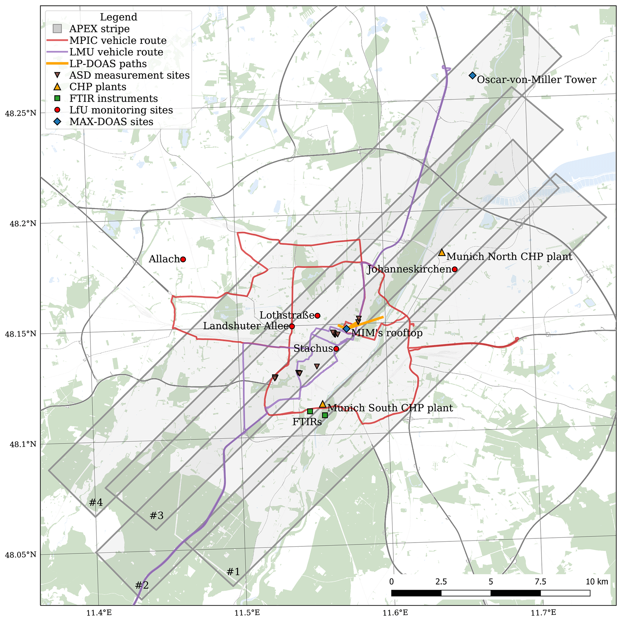
Figure 1 Map of Munich with overlaid APEX flight stripes (nos. 1–4), routes taken by the LMU and MPIC vehicles in the afternoon of 7 July 2016, as well as locations of combined heat and power (CHP) plants, Fourier transform infrared (FTIR) instruments, LfU monitoring sites, and stationary MAX-DOAS instruments and the locations of surface reflectance measurements with the ASD instruments. Map data from © OpenStreetMap contributors 2021. Distributed under the Open Data Commons Open Database License (ODbL) v1.0.

2.4 Stationary MAX-DOAS

NO₂ profiles above roof level were measured with a MAX-DOAS instrument at the MIM's rooftop in the city center and a second MAX-DOAS instrument on top of the OvM tower about 15 km northeast of the city center. Unfortunately, no measurements are available at the OvM tower for 7 July 2016 due to technical issues of the instrument.

The MAX-DOAS was programmed to measure scattered solar radiances at nine elevation angles (2, 3, 4, 5, 6, 8, 15, 30, and 90^∘) and seven azimuth angles (0, 90, 135, 180, 225, 270, and 315^∘). In this study, only measurements at an azimuth angle of 0^∘ (pointing northwards) were analyzed, from which differential NO₂ slant columns (dSCDs) were retrieved using a DOAS analysis for a wavelength range from 425 to 490 nm. The DOAS analysis considered NO₂, O₄, O₃, and H₂O absorption cross sections, a Ring spectrum, as well as a polynomial of degree 5. Small shift and squeeze of the wavelength are allowed in the wavelength mapping process to compensate for small uncertainties caused by the instability of the spectrograph.

Aerosol extinction coefficient profiles were retrieved from the O₄ absorption bands at 477 nm using the Munich Multiple wavelength MAX-DOAS retrieval algorithm (M³), described in detail in Chan et al. (2018, 2019, 2020). Due to the systematic discrepancy between observation and model simulation of O₄ DSCDs (e.g., Wagner et al., 2009), all MAX-DOAS observations of O₄ DSCDs are multiplied by a correction factor of 0.8 (see Chan et al., 2019, for details). The algorithm uses the optimal estimation method (Rodgers, 2000) and the libRadtran radiative transfer code as the forward model (Mayer and Kylling, 2005; Emde et al., 2016). The aerosol profiles obtained from the procedure are used for the calculation of air mass factors for discrete vertical layers (1D-layer AMFs) required for NO₂ profile inversion. The layer AMFs are calculated at 477 nm for the retrieval of NO₂ profiles using the Monte Carlo solver (MYSTIC) of libRadtran (Emde et al., 2016; Schwaerzel et al., 2020).

2.5 Airborne Prism Experiment (APEX)

APEX is a push-broom imaging spectrometer that has been developed for environmental monitoring (Schaepman et al., 2015). It measures radiance spectra with an optimized integration time simultaneously in 1000 across-track spatial pixels within a 28^∘ field of view. At a flight altitude of 7360 m above ground, its spatial resolution is about 4 m × 6 m in the across- and along-track directions, respectively. The along-track resolution is computed from aircraft altitude, ground speed, and integration time. For each pixel, spectral radiance is measured in the visible and near-infrared (VNIR, 372–1015 nm) and shortwave infrared (SWIR, 940–2540 nm) channels. To retrieve NO₂ VCDs, spectra were acquired in the unbinned mode, providing the highest nominal spectral resolution of 0.86 nm full width at half maximum (FWHM) and 0.45 nm spectral sampling interval (SSI) in the VNIR channel with 334 spectral bands. Note that FWHM and SSI vary with wavelength and range from 0.86 to 15 nm (FWHM) and from 0.45 to 7.5 nm (SSI), owing to the dispersion characteristics of the VNIR prism.

The APEX measurements were acquired along four pre-defined stripes shown in Fig. 1 on 7 July 2016 in the early afternoon (14:16–14:56 CEST). The four stripes cover a large fraction of the city, with a large overlap between the stripes to increase the number of APEX observations in the city center, where most ground-based observations were conducted. In addition, the stripes cover forest and agriculture land, which were used as background spectra in the DOAS retrieval.

APEX NO₂ retrieval algorithms were developed at Empa in Switzerland (Popp et al., 2012) and at BIRA in Belgium (Tack et al., 2017) using the QDOAS software for the DOAS analysis and the LIDORT radiative transfer model for AMF computations. In this study, we used a new version of the Empa APEX NO₂ retrieval algorithm, which has been completely rewritten using Python, allowing for automatic and parallel processing of APEX measurements. The new version uses the Python library flexDOAS for the DOAS analysis (Kuhlmann, 2022) and the Monte Carlo MYSTIC solver for AMFs (Schwaerzel et al., 2020).

To increase the signal-to-noise ratio for the NO₂ retrieval, 20 × 10 APEX pixels were spatially binned in the across- and along-track directions, respectively. As a result, the spatial resolution of the APEX instrument is reduced to about 80 m × 60 m. An in-flight spectral calibration was conducted to improve the accuracy of center wavelength positions and the FWHM of the instrument's slit function (Kuhlmann et al., 2016). This was required because the default spectral calibration provided by the APEX processing and archiving facility (Hueni et al., 2009, 2013) was not sufficiently accurate for the retrieval of NO₂.

NO₂ dSCDs were retrieved from the spatially binned APEX spectra using flexDOAS. The last 50 spectra at the western end of each stripe were used as a reference spectrum for each across-track position. The DOAS analysis was applied to a window from 470 to 510 nm where we fitted NO₂ and O₄ absorption cross sections, a Ring spectrum, a five-degree polynomial, as well as a relative offset fitted as a quadratic polynomial that was subtracted from both the measurement and reference spectra. The cross sections of O₃ and H₂O are not considered due to cross-correlations and overparameterization in the small fitting window (Popp et al., 2012; Tack et al., 2017).

The NO₂ dSCDs are the differences between SCDs in the observation and reference spectra,

$$\begin{array}{}\text{(1)}& \mathrm{dSCD}=\mathrm{SCD}-{\mathrm{SCD}}_{\mathrm{ref}},\end{array}$$

which are solved for tropospheric VCDs using $\mathrm{SCD}=\mathrm{AMF}\cdot \mathrm{VCD}$ as

$$\begin{array}{}\text{(2)}& \mathrm{VCD}={\displaystyle \frac{\mathrm{dSCD}+{\mathrm{VCD}}_{\mathrm{ref}}\cdot {\mathrm{AMF}}_{\mathrm{ref}}}{\mathrm{AMF}}},\end{array}$$

where VCD_ref and AMF_ref are the reference VCDs and AMFs for each across-track position. Mobile MAX-DOAS observations conducted in the reference area during the APEX flight were used as reference VCDs (VCD_ref).

To calculate the AMFs, 1D-layer AMFs were computed with the MYSTIC solver of the libRadtran model (Emde et al., 2016; Schwaerzel et al., 2020) depending on Sun position, instrument viewing direction, surface reflectance, surface elevation, and atmospheric scattering by molecules and aerosols using a US standard atmosphere. Surface reflectances were taken from the APEX surface reflectance product at 490 nm (cf. Sect. 2.8) in the center of the DOAS fitting window assuming Lambertian equivalent reflectance (LER). Aerosol scattering was included using an aerosol optical depth of 0.10 measured by the AERONET station on the MIM's rooftop and libRadtran's default aerosol profile. Total AMFs were computed from the 1D-layer AMFs using the NO₂ profile measured by the MAX-DOAS instrument on the MIM's rooftop.

The APEX NO₂ VCDs were destriped to account for small variations of dSCDs and true VCD_ref in the across-track direction by subtracting deviations from a cubic polynomial fitted to the mean across-track VCDs. In addition, we performed a bias correction between the different aircraft overpasses by adding a constant offset to each stripe so that the mean values of the overlapping parts of two neighboring stripes are identical. Both the across-track variations as well as the difference between stripes are mainly caused by differences in spectral and radiometric calibration (Kuhlmann et al., 2016). The NO₂ VCDs were then mapped onto a longitude–latitude grid with about 10 m resolution for comparison with the ground-based observations using the gridding algorithm of Kuhlmann et al. (2014) (Code repository: Kuhlmann, 2021b).

The uncertainties in NO₂ VCDs were calculated as the quadratic sum of the uncertainties in dSCDs, AMFs, and SCD_ref:

$$\begin{array}{}\text{(3)}& {\mathit{\sigma }}_{\mathrm{VCD}}=\sqrt{{\left({\displaystyle \frac{{\mathit{\sigma }}_{\mathrm{dSCD}}}{\mathrm{AMF}}}\right)}^{\mathrm{2}}+{\left({\displaystyle \frac{{\mathit{\sigma }}_{{\mathrm{SCD}}_{\mathrm{ref}}}}{\mathrm{AMF}}}\right)}^{\mathrm{2}}+{\mathit{\sigma }}_{\mathrm{AMF}}^{\mathrm{2}}{\left({\displaystyle \frac{\mathrm{VCD}}{\mathrm{AMF}}}\right)}^{\mathrm{2}}},\end{array}$$

where σ_dSCD was estimated from the DOAS analysis. The uncertainties in AMFs and SCD_ref were estimated from the comparison with the ground-based remote sensing observations conducted during the campaign.

2.6 Mobile measurements

Mobile measurements were conducted with two vehicles operated by MPIC and LMU, respectively. Each vehicle was equipped with an in situ instrument measuring near-surface concentrations (CE-DOAS and CAPS) and a spectrometer measuring NO₂ column densities (Tube and Mini MAX-DOAS) (see Table 1). The measurements were conducted along varying routes in the city. The MPIC vehicle mostly drove circles in the city center to capture the NO₂ fields in across-track direction of the APEX measurements, while the LMU vehicle drove from the southwest to the northeast of the city along the highway or on smaller roads in the city center to sample in the along-track direction of APEX.

2.6.1 Mobile in situ instruments

Near-surface NO₂ concentrations were measured with two highly sensitive and specific in situ instruments: first a T500U CAPS NO₂ analyzer from Teledyne API that is routinely used in the Swiss National Air Pollution Monitoring Network (NABEL). CAPS consists of a blue LED, a measurement chamber with two highly reflective mirrors, and a vacuum photodiode detector. The instrument uses the CAPS technique to directly measure NO₂ (Kebabian et al., 2005, 2008). CAPS was installed in the LMU vehicle with the sample inlet fixed at the roof of the vehicle at about 2 m height. The NO₂ concentrations were recorded every 2 s.

The second instrument applied broadband cavity enhanced differential optical absorption spectroscopy (CE-DOAS), which uses a blue LED, a measurement chamber, and a spectrometer to obtain NO₂ concentrations using the DOAS technique between 435.6 and 455.1 nm (Platt et al., 2009; Zhu et al., 2020). The CE-DOAS was installed in the MPIC vehicle with the inlet located at the front right window of the vehicle at 1.5 m above the ground, and measurements were recorded every 2 s.

CAPS and CE-DOAS agreed well when operated together on the LMU vehicle on 1 and 4 July 2016. Pearson correlation coefficients were 0.995 and 0.984, and root mean square errors (RMSEs) were 6.1 and 5.9 ppbv on the two days. The differences between CAPS and CE-DOAS are due to instrument differences such as length of tubing and integration times, the short measurement interval of 2 s, and the high variability of NO₂ concentrations on roads. Furthermore, it was necessary to shift CAPS measurements by 16.9 and 5.6 s, respectively (Fig. S2). The time differences were caused by non-synchronized computer clocks and the differences in tubing and integration times. On campaign day, GPS times were used to minimize time differences between instruments.

2.6.2 Mobile MAX-DOAS measurements

The mobile MAX-DOAS measurements were carried out using two instruments operated by MPIC: the Tube MAX-DOAS, which was mounted on the MPIC vehicle, is a scientific grade instrument with a high signal-to-noise ratio and stable spectroscopic properties (see, e.g., Kreher et al., 2020). The Mini MAX-DOAS is a more compact instrument but with a lower signal-to-noise ratio and less stable spectral properties (see, e.g., Shaiganfar et al., 2011). This instrument was mounted on the LMU vehicle. Because of the different signal-to-noise ratios, the total integration times for individual measurements were set to 30 s for the Tube MAX-DOAS and 60 s for the Mini MAX-DOAS instruments, respectively. The obtained spectra are averages of multiple single measurements with integration times adjusted according to current sky conditions. Mean individual integration times were roughly 65 ms, leading to numbers of scans of roughly 460 and 920 for the two instruments, respectively. One complete elevation sequence contained six (Tube MAX-DOAS) or seven (Mini MAX-DOAS) measurements at a low (22^∘) elevation angle, followed by one measurement in the zenith direction. The line of sight of the Mini MAX-DOAS instrument was in the driving direction and the one of the Tube MAX-DOAS instrument was directed backwards with respect to the driving direction. NO₂ was analyzed in the spectral range from 400 to 439 nm using a fixed daily Fraunhofer reference measured in the zenith direction. Only results with root mean square (rms) values below $\mathrm{8}\times {\mathrm{10}}^{-\mathrm{4}}$ (Tube MAX-DOAS) and below $\mathrm{2}\times {\mathrm{10}}^{-\mathrm{3}}$ (Mini MAX-DOAS) were considered for further processing. The method described in Wagner et al. (2010) and Ibrahim et al. (2010) was applied to determine the NO₂ absorption in the Fraunhofer reference spectrum and to correct for the changing stratospheric NO₂ absorption.

2.7 Fourier transform infrared (FTIR) spectrometers

Two ground-based FTIR spectrometers were deployed near the Munich South CHP plant to measure column-averaged dry air mole fractions of CO₂ and CH₄ (XCO₂ and XCH₄). The instruments are owned by the Karlsruhe Institute of Technology (KIT) and Technical University of Munich (TUM) and are identified as EM27 KIT and EM27 TUM, respectively. Both instruments are operated by TUM.

The compact and mobile solar-tracking FTIR spectrometers (Bruker EM27/SUN, Gisi et al., 2012) point towards the Sun during measurements and measure spectra in the wavenumber range from 6000 to 9000 cm⁻¹. By placing one spectrometer upwind and the other downwind of the CHP plant, differential column measurements (DCMs) can be used to determine the CO₂ and CH₄ emissions from this source. DCMs have proven to be an effective method for determining emissions from different types of sources (Hase et al., 2015; Chen et al., 2016; Dietrich et al., 2021; Toja-Silva et al., 2017; Zhao et al., 2019). Differential column measurements exhibit a very high precision of 0.01 % for XCO₂ and XCH₄ at a 10 min integration time (Chen et al., 2016; Hedelius et al., 2016).

To capture the emission plume, the spectrometers were placed based on the forecasted wind direction. On 7 July 2016, the wind was blowing from the northwest in the morning, turning to northeast in the afternoon. One spectrometer was placed southwest of the CHP plant to capture the plume in the morning and the other spectrometer south to capture the plume at noon. As a result, the stations acted alternately as downwind sites and as background sites throughout the day.

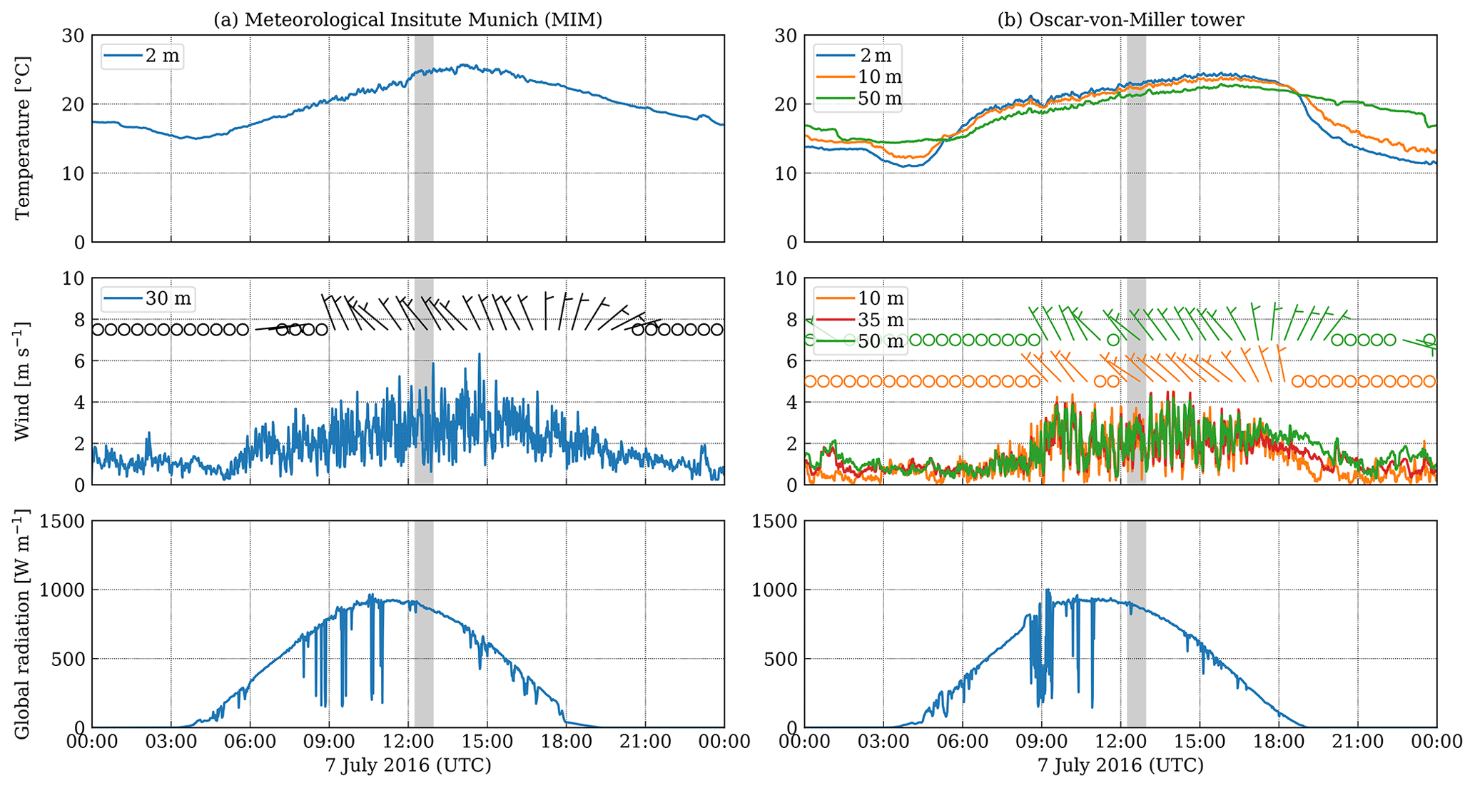
Figure 2 Time series of meteorological observations (temperature, wind speed and direction, and global radiation) at (a) the Meteorological Institute Munich (MIM) and at (b) the Oscar-von-Miller (OvM) tower. The APEX flight time is shown as a gray area.

2.8 Surface reflectance

Surface reflectance is a critical input parameter for the AMF computation, because uncertainties in the reflectance can have a strong impact on the NO₂ VCDs. The APEX reflectance product calculates hemispheric–conical reflectance factors (HCRFs; Schaepman-Strub et al., 2006) using the atmospheric correction software ATCOR-4 (Richter and Schläpfer, 2002). In short, atmospheric water vapor and aerosol optical depth are estimated from APEX radiance data, which are used, together with other parameters describing the Sun-observer geometry, to obtain representative atmospheric transfer functions (e.g., transmittance, spherical albedo, path radiance). The transfer functions were pre-calculated with MODTRAN-5 (Berk et al., 2005) and stored in a look-up table. Radiance data are also used to estimate spectral non-uniformities (e.g., spectral shift, band broadening). This information is essential to spectrally convolve identified atmospheric transfer functions and eventually retrieve HCRFs.

To evaluate the APEX surface reflectance product, HCRF spectra were collected with a handheld analytical spectral device (ASD) field spectroradiometer during the campaign. In total, 14 spectra were measured on 7 July 2016 from 11:05 to 16:19 CEST. All ASD measurements were located in the second and third APEX stripes and included surfaces of varying types and brightnesses. The locations are shown in Fig. 1, and details are listed in Table S1.

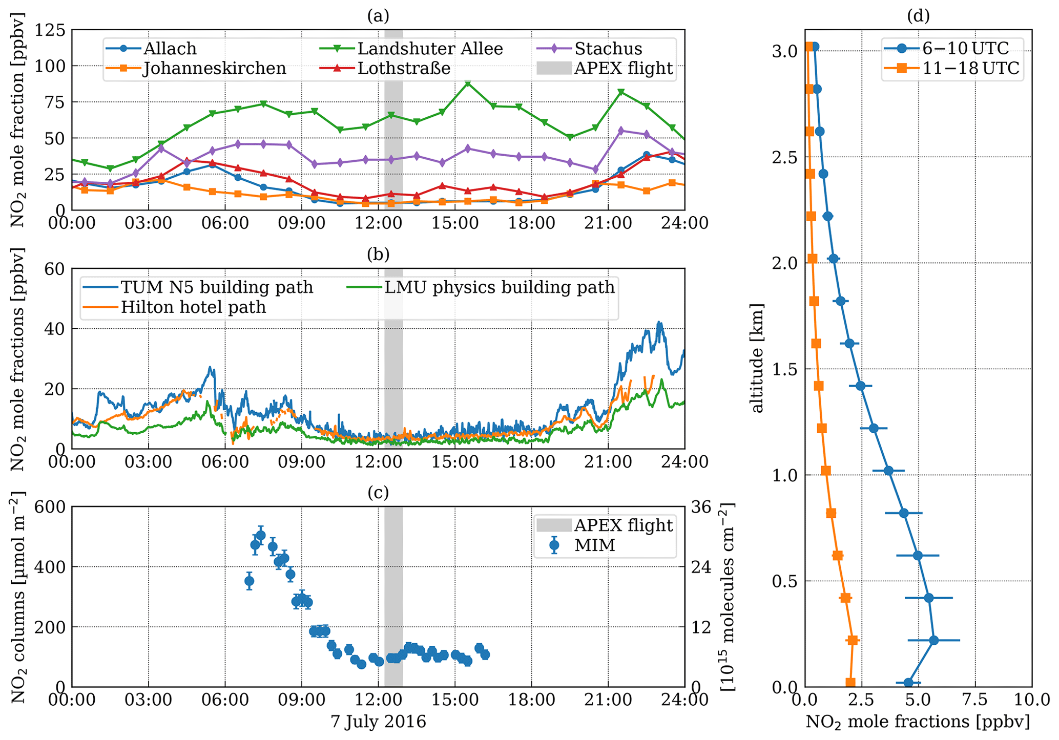
Figure 3 Time series of NO₂ mole fractions from (a) monitoring stations and (b) the LP-DOAS systems. (c) Time series of vertical column densities and (d) mean NO₂ profiles from the MAX-DOAS instrument on the MIM's rooftop on 7 July 2016.

3 Results

3.1 Campaign day with APEX overpass

The APEX flight window was part of a larger measurement campaign in June and July 2016 with various targets. The choice of a suitable day for Munich is based mainly on flight permission and weather conditions. The first 2 weeks of July 2016 were mostly cloudy, with daily mean temperatures and wind speeds ranging from 12 to 27 ^∘C and from 1.0 to 3.9 m s⁻¹, respectively. A favorable situation with almost no clouds was predicted for 7 July 2016 for the area of Munich, which allowed us to conduct the APEX measurements in the early afternoon (14:16–14:56 CEST).

Figure 2 shows the time series of meteorological parameters (temperature, wind speed and direction, and global radiation) measured at MIM and at the OvM tower on this day. In the morning, small cumulus clouds were still present over Munich, which can be seen as a reduction in global radiation. In the afternoon, the clouds mostly vanished, making it possible to conduct the APEX flight. Figure S3 shows the true color composite of the APEX measurements, showing only a small cloud at the edges of the image.

Wind speeds were low during night (about 1 m s⁻¹) and slightly higher and highly variable during the day (1 to 6 m s⁻¹). The wind directions were mostly northwesterly during day, turning to northeasterly in the evening. We estimated the dispersion category during daytime as very unstable (category V) based on the procedure published by the Association of German Engineers, which determines dispersion categories based on tabulated values for wind speed, cloud fraction, and hour of day (VDI – Fachbereich Umweltmeteorologie, 2009, Annex A). Wind speed and direction are consistent with the simulations from the COSMO-1 and COSMO-7 analysis products provided by MeteoSwiss with 1 and 7 km spatial resolution, respectively (Fig. S11). The COSMO-1 model with about 1 km resolution shows small convective cells with highly variable 10 m wind speeds over Munich with a similar spatial variability to the temporal variability of the ground measurements.

Figure 3a shows the time series of NO₂ NSCs at the monitoring stations on 7 July 2016. The NO₂ measurements show a morning peak during rush hour and an increase in the evening when the boundary layer becomes stable again, solar radiation is missing, and the sources (traffic) are still active. The APEX flight was performed around the time of the lowest NSCs. Concentrations were about 5 ppbv at the two suburban background stations (Allach and Johanneskirchen) and somewhat higher at 11 ppbv at the urban background station (Lothstraße). Different from these stations, the two urban traffic stations showed only little variations during the day due to their proximity to emission sources. Concentrations during the APEX flight were 35 and 66 ppbv at Stachus and Landshuter Allee, respectively. The LP-DOAS also measured the diurnal cycle with molar fractions similar to the suburban background stations due to the elevated light paths measuring NO₂ above the urban canopy. The LP-DOAS measured NO₂ concentrations of about 5 ppbv during the APEX overpass.

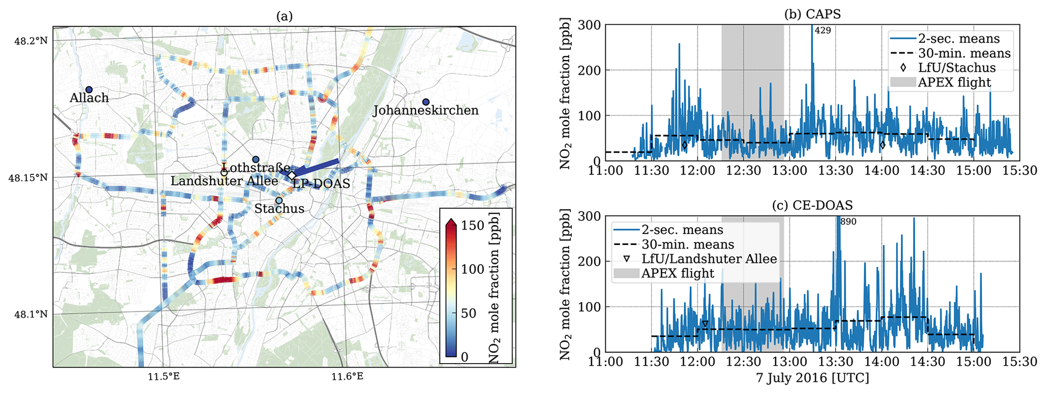
Figure 4 (a) Map of NO₂ mole fractions measured by LMU and MPIC vehicles in the afternoon. Locations of the LfU monitoring stations are shown as circles colored by the mean afternoon NO₂ mole fraction. Panels (b) and (c) show the time series of NO₂ mole fractions measured by the CAPS and CE-DOAS instruments on the LMU and MPIC vehicles, respectively. Map data from © OpenStreetMap contributors 2021. Distributed under the Open Data Commons Open Database License (ODbL) v1.0.

The MAX-DOAS instrument on the rooftop (Fig. 3c) measured the highest NO₂ VCDs in the early morning, with up to 504 µmol m⁻². NO₂ VCDs dropped substantially to about 104±15 µmol m⁻² in the afternoon. Note that 100 µmol m⁻² is about 6 × 10¹⁵ molec. cm⁻². Since the temporal variability of NO₂ VCDs was small in the afternoon, differences between mobile and APEX measurements due to different measurement times are likely small.

Figure 3d shows averaged NO₂ profiles retrieved in the morning and in the afternoon. The profiles were retrieved for an azimuth angle of 0 degrees, i.e., looking northwards. The mole fractions in the lowest layer (0–200 m) were only 4.6 and 2.0 ppbv in the morning and afternoon, respectively, which is smaller than the 8.4 and 3.8 ppbv measured by the LP-DOAS system on average. The averaging kernels of MAX-DOAS retrieval for the lowest layer range between 0.85 and 1, indicating the retrieval reconstructs the lowest layer quite well. However, the lowest layer of MAX-DOAS represents the average of the lowest 200 m, while LP-DOAS measures at about 30 m above ground. Therefore, it is expected that LP-DOAS will measure higher concentrations than MAX-DOAS.

3.2 Mobile in situ measurements

Figure 4a shows the NO₂ mole fractions along the routes taken by the LMU and MPIC vehicles on 7 July 2016 in the afternoon. The markers for the LfU sites and lines for LP-DOAS show mean values in the afternoon (11:00–17:00 UTC). Figure 4b and c show the corresponding time series of NO₂ mole fractions. A corresponding figure showing measurements during the morning (07:00–10:00 UTC) is available in Fig. S4.

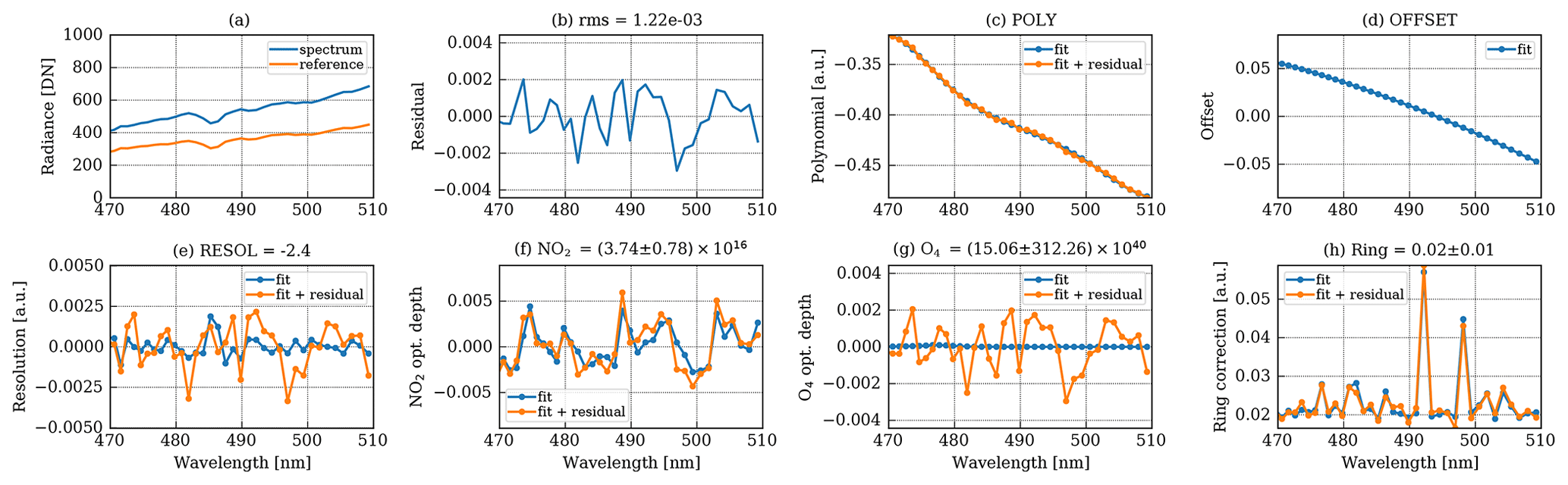
Figure 5 Example of DOAS retrieval for APEX stripe no. 2 inside the NO₂ plume of the Heizkraftwerk Süd power plant at across- and along-track positions of 42 and 314, respectively: (a) APEX measurement spectrum and reference spectrum, (b) residual, (c) fitted polynomial, (d) fitted offset, (e) resolution cross section, (f) NO₂ optical depth, (g) O₄ optical depth, and (h) Ring pseudo cross section.

NO₂ mole fractions varied strongly along the route because they are very sensitive to local emissions. The values ranged from 0 to 890 ppb, with highest values being observed in congested areas, in front of traffic lights, or in tunnels. While 2 s values show high variability along the road, 30 min averages are similar to hourly measurements at the roadside stations at Stachus and Landshuter Allee when the vehicle passed at distances of 75 m and <10 m from the stations, respectively (Fig. 4b and c). A more detailed comparison of mobile measurements and measuring stations for these data can be found in Zhu et al. (2020).

3.3 APEX NO₂ observations

3.3.1 APEX NO₂ retrieval algorithm

The true color images of the four APEX stripes are shown in Fig. S3. The stripes were mostly cloud-free, with only a small cumulus cloud on the western edge of the second stripe.

The spectral calibration was much more stable than on other flights investigated by Kuhlmann et al. (2016), likely because the measurements were conducted after the long transfer flight from Zurich to Munich prior to the measurements, allowing the system to reach a stable pressure and temperature state. The in-flight spectral calibration shows the known spectral smile of the APEX instrument in the across-track direction (Fig. S5a) but no strong drift during data acquisition in the along-track direction (Fig. S5b). The instrument slit function is about 30 % wider in-flight than the laboratory calibration (see Sect. 2.5), which is a known but not fully understood characteristic of the APEX instrument that is likely related to stray light and vignetting (Kuhlmann et al., 2016).

Figure 5 shows an example of the DOAS analysis for an APEX pixel acquired inside the plume of the Munich South CHP plant (stripe: 2, across-track: 42, along-track: 314) with a root mean square (rms) of $\mathrm{1.22}\times {\mathrm{10}}^{-\mathrm{3}}$ and an NO₂ dSCD of 621±130 µmol m⁻².

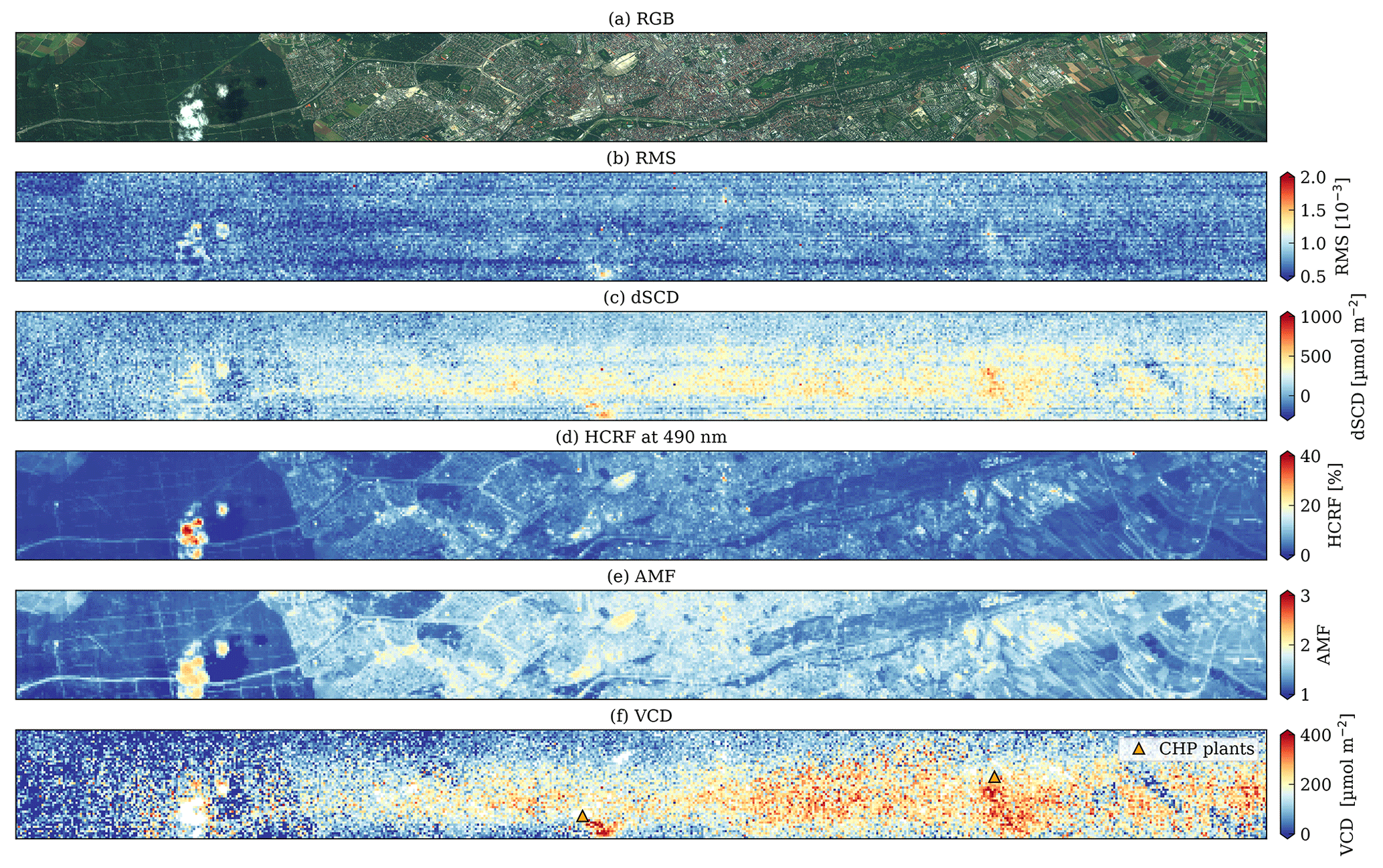
Figure 6 (a) True color image, (b) rms, (c) NO₂ differential slant column densities (dSCDs), (d) hemispheric–conical reflectance factors (HCRFs), (e) air mass factors (AMFs), and (f) NO₂ vertical column densities (VCDs) of the second APEX stripe (see Fig. 1).

The distributions of rms, dSCDs, HCRFs, AMFs, and VCDs are shown in Fig. 6 for the second stripe. The distributions for the other APEX stripes are shown in Figs. S6–S8.

For all stripes, rms values do not vary strongly spatially, ranging from 0.49 to $\mathrm{1.00}\times {\mathrm{10}}^{-\mathrm{3}}$ (5th to 95th percentiles) with a mean value of $\mathrm{0.73}\times {\mathrm{10}}^{-\mathrm{3}}$. The values are smallest in the area used for computing the reference spectra (Fig. 6a). The rms values are highest over very bright surfaces and increase with distance from the reference area. This dependency on along-track position is likely caused by a mismatch in spectral calibrations between the reference and measurement spectra that increases with distance from the reference area. The rms values also vary in the across-track direction, where positions have a higher rms than others, also likely caused by small differences in the spectral calibration.

The NO₂ dSCDs show no clear spatial pattern, but values are highest in the middle over the city and lowest on the right-hand side over the forest used as the reference area (Fig. 6b). The average dSCD is 178 µmol m⁻², but values range between −71 and 417 µmol m⁻² (5th to 95th percentiles).

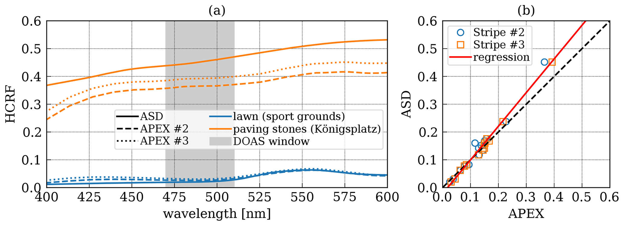
Figure 7 (a) APEX and ASD HCRF spectra for a dark and bright surface. (b) Scatter plot comparing APEX and ASD at 490 nm over all 14 targets. The regression line has a slope of 1.211 and an intercept of −0.022. The correlation coefficient is 0.99.

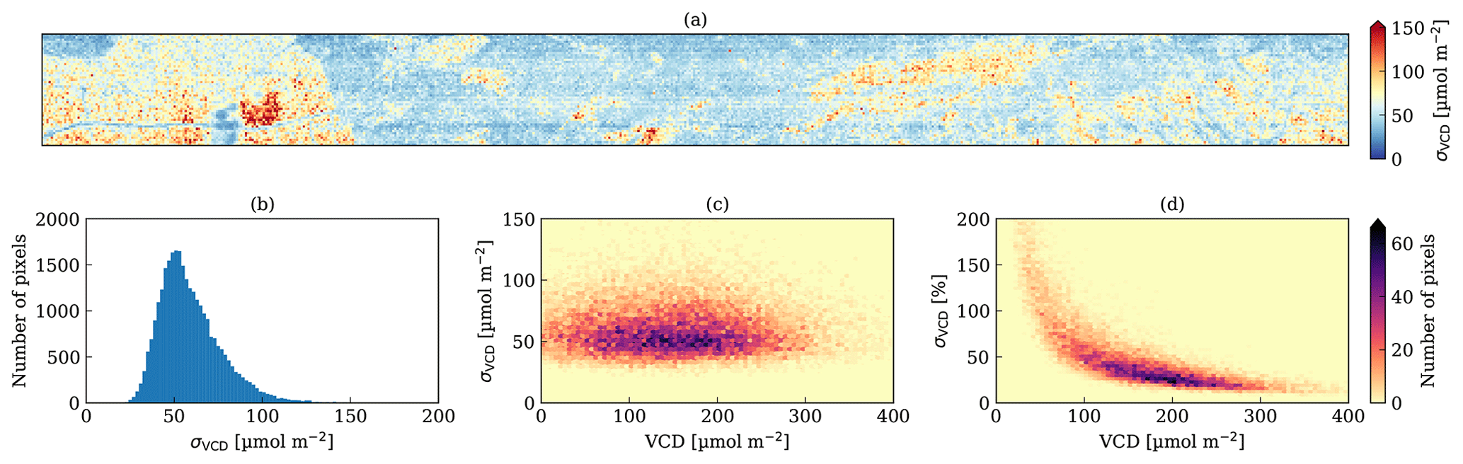
Figure 8 Estimated uncertainty of NO₂ VCDs for the second APEX stripe showing (a) the spatial distribution (see Fig. 1) and (b) the distribution of uncertainties and the dependency on the NO₂ VCDs of the (c) absolute and (d) relative uncertainties.

HCRFs at 490 nm in the APEX product varied over the city from 0.02 to 0.12 (5th to 95th percentiles), with a mean of 0.06. The HCRFs were smaller, with an average value of 0.03 (range: 0.01–0.06) over the forest in the west of the city, which was used as a reference area for the DOAS analysis. The AMFs depend mainly on HCRFs and range between 1.1 and 1.9 with an average of 1.5 (Fig. 6d).

The NO₂ VCDs computed from dSCDs and VCDs (Eq. 2) have an average of 115 µmol m⁻² and range from −37 to 294 µmol m⁻² (5th to 95th percentiles). The destriping algorithm successfully removes the stripes visible in the dSCDs (Fig. 6e). The destriped VCD field shows clearer features, such as two enhancements in the left and center of the stripe which match the locations of the Munich North and Munich South CHP plants.

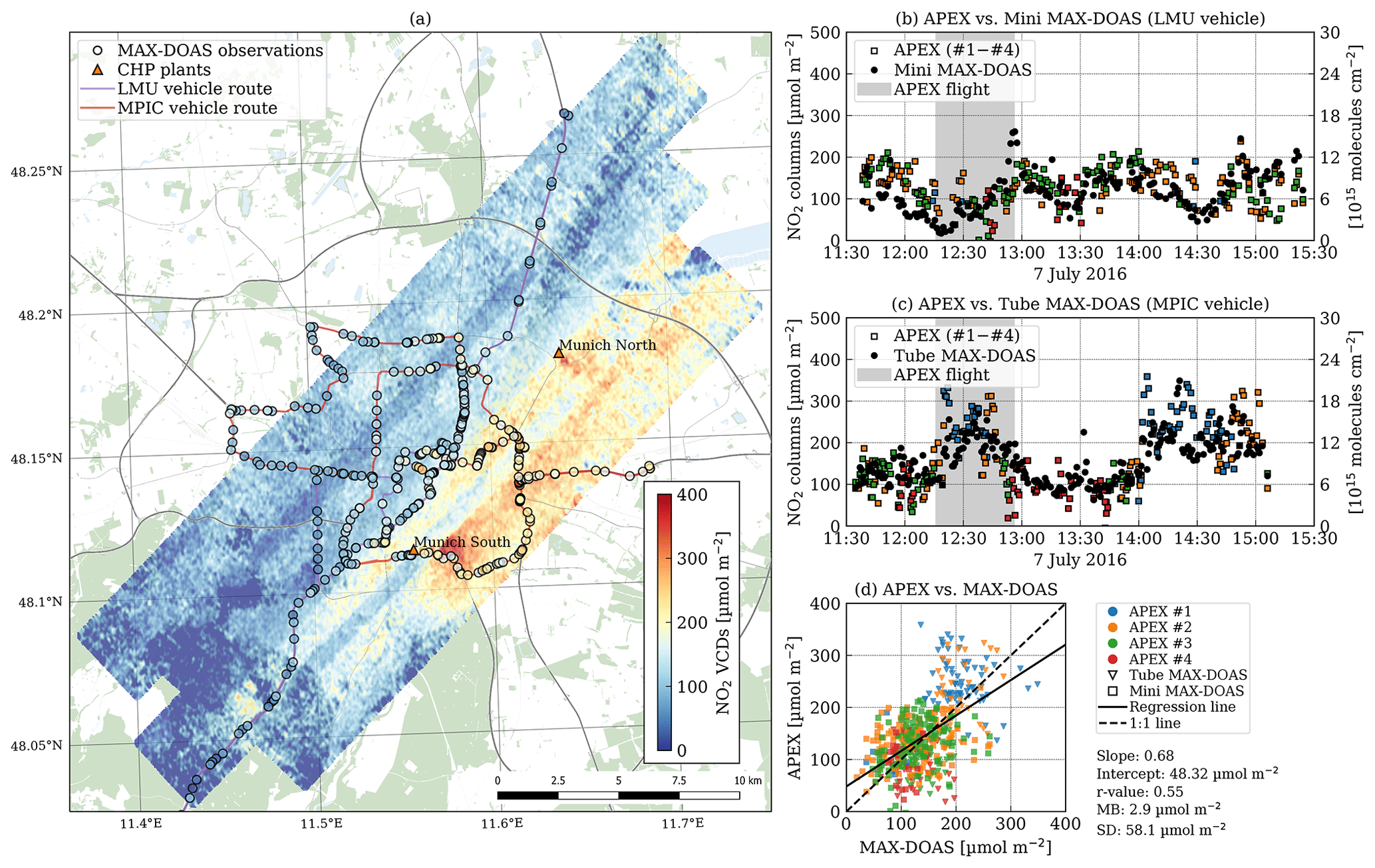
Figure 9 (a) Map NO₂ VCDs from APEX and mobile MAX-DOAS measurements on 7 July 2016 (afternoon). (b, c) Time series of spatially co-located APEX and (b) Mini MAX-DOAS and (c) Tube MAX-DOAS VCDs. (d) Scatter plot showing MAX-DOAS and APEX NO₂ VCDs for spatially co-located observations. Map data from © OpenStreetMap contributors 2021. Distributed under the Open Data Commons Open Database License (ODbL) v1.0.

3.3.2 APEX NO₂ uncertainties

The uncertainties of the VCDs were obtained from the uncertainties of dSCDs, SCD_ref, and AMFs (Eq. 3). The dSCD uncertainty was obtained directly from the DOAS fitting routine and varied between 18 and 185 µmol m⁻² with 56 µmol m⁻² on average.

The uncertainties in the AMFs are caused mainly by uncertainties in the surface reflectance product and the a priori NO₂ profile used in AMF calculations. To estimate the uncertainty of the APEX surface reflectance product, we validated the product with the 14 ASD measurements in the city center covered by the second and third APEX stripes (Figs. 1 and S9, and Table S1). Figure 7 shows two examples of HCRF spectra over a dark and bright surface. APEX and ASD HCRF agree very well at 490 nm, with a correlation coefficient of 0.99, but the APEX product tends to underestimate high reflectances (slope: 1.21, intercept: −0.02). The root mean square difference (RMSD) between APEX and ASD HCRFs is 0.014 considering only ASD values smaller than 0.30, which is a relative uncertainty of about 23 % for the mean HCRF over the city (HCRF = 0.06). We computed the 1σ uncertainties of the AMFs using an uncertainty of 0.014 in HCRFs, which results in AMF uncertainties of 0.15 and 0.08 for HCRFs of 0.03 and 0.06, respectively.

The uncertainties in the a priori NO₂ profiles translate to about 10 % uncertainty in AMFs for satellite NO₂ products (e.g., Boersma et al., 2011). In our study, the a priori NO₂ profile was obtained from the MAX-DOAS instrument on the MIM rooftop, which should provide a representative profile for the city above building level. Since the instrument is not sensitive to near-surface NO₂, we analyzed the impact of the NO₂ profile sensitivity by replacing the mole fraction in the lowest layer (0–200 m) with values ranging from 0 to 100 ppbv. We find that the corresponding AMF uncertainty is smaller than 0.10 for LERs larger than 0.20 and up to 0.16 for a black surface (LER = 0.00).

The total AMF uncertainties are obtained as a sum of variances of the individual components (surface reflectance and the a priori NO₂ profile). We calculated that AMF uncertainties decrease from 0.40 to 0.10 when LERs increase from 0.00 to 0.05 and are constant at 0.10 when LERs are larger than 0.05. Uncertainties might be somewhat larger because uncertainties in the aerosol profiles are not taken into account.

The uncertainty of the reference slant column density (SCD_ref) was estimated to be about 25 % considering the uncertainty of the VCDs retrieved from the Mini MAX-DOAS (σ_SCD<15 %) and the uncertainty of the AMFs averaged over the forest used as the reference area (σ_AMF≈0.13).

The VCD uncertainties were computed from Eq. (3). The uncertainty is dominated by the dSCD uncertainty that accounts for 87 % of total uncertainty due to the low signal-to-noise ratio of the APEX measurements. The second-most important term is the AMF uncertainty accounting for 12 % of the total uncertainty, while the uncertainty of the reference SCD is small compared to the other two components. Figure 8a shows the estimated uncertainties for the second stripe. The uncertainties are highest over dark surfaces (forest, parks, and water surfaces), because the uncertainty inversely depends on AMFs (Eq. 3). The uncertainty ranges from 34 to 86 µmol m⁻² (5th–95th percentiles), with an average of 56 µmol m⁻² (Fig. 8b). Since the uncertainty depends on VCDs, uncertainties slightly increase with VCDs (Fig. 8c).

3.3.3 APEX NO₂ map

Figure 9a shows the map of NO₂ VCDs from the APEX instrument. A Gaussian smoothing filter (σ≈50 m) was applied to reduce spatial noise. The map shows lower values in the northwest upwind and higher values in the southeast downwind of the city center. The locations of the Munich North and Munich South CHP plants are marked by two orange triangles. The emission plumes of both CHP plants are clearly visible in the APEX data. Otherwise, no small-scale structures, such as roads, can be identified on the map.

While local enhancements related to traffic such as key intersections and highways could be identified in previous APEX campaigns (e.g., Popp et al., 2012; Tack et al., 2017), such structures are missing in Munich, likely due to the high variability in wind speed and direction resulting in strong spatial mixing. Recent model studies demonstrate that this is also partially explainable by 3D radiative transfer effects (Schwaerzel et al., 2021).

The APEX NO₂ product also shows artifacts near the stripe edges that are likely related to insufficient knowledge about the spectral calibration and vignetting that affect the accuracy of the instrument slit function (Kuhlmann et al., 2016). The NO₂ map also shows unrealistic low values over water surfaces that have also been noticed by Tack et al. (2017).

Figure 10 (a) Map of ratios of NO₂ NSCs (µmol m⁻³) to VCDs (µmol m⁻²) measured by in situ monitors and MAX-DOAS on board the LMU and MPIC vehicles. (b) The time series of ratios measured with the two vehicles and (c) a scatter plot of NSCs and VCDs. Map data from © OpenStreetMap contributors 2021. Distributed under the Open Data Commons Open Database License (ODbL) v1.0.

3.4 Comparison of APEX and MAX-DOAS observations

Figure 9b and c show the time series of spatially but not temporally collocated APEX and MAX-DOAS NO₂ VCDs, which were obtained by averaging the APEX values along the vehicle paths ±30 and ±15 s for the Mini and Tube MAX-DOAS, respectively. The LMU vehicle drove along the magenta line (Fig. 9a), leaving the urban area in the southeast and northwest. The time series shows local NO₂ minima when the vehicle was at the southwestern border of the APEX map at 12:20 and 14:35 UTC and at the northwestern border of the APEX map at 13:25 UTC. The MPIC vehicle was driving in a counterclockwise direction around the city center along the red line in Fig. 9a. NO₂ VCDs were highest when the vehicle was located in the eastern part of the city (12:30 and 14:30 UTC). A map showing the time labels is provided in Fig. S10.

In total, 518 co-located APEX and MAX-DOAS observations are available. APEX and MAX-DOAS NO₂ VCDs agree with a moderate correlation coefficient r of 0.55. The regression line has a slope of 0.68 and an intercept of 48.3 µmol m⁻². Furthermore, the mean bias (MB) computed from the differences between APEX and MAX-DOAS measurements is close to zero, at 2.9 µmol m⁻². The standard deviation (SD) of the differences is 58.1 µmol m⁻². The discrepancy between airborne and ground-based observations is largely explainable by the relatively high uncertainty of individual APEX and MAX-DOAS NO₂ VCDs (i.e., APEX uncertainties were approximately 60 µmol m⁻²). In addition, airborne and ground-based instruments do not measure exactly the same air mass due to different viewing directions and different measurement times. Furthermore, the vertical sensitivity to NO₂ is different for APEX and MAX-DOAS, so that inconsistent assumptions about the vertical profile of NO₂ affects the comparison. It should be noted that APEX and MAX-DOAS observations are not fully independent, because the APEX NO₂ retrieval algorithm uses MAX-DOAS measurements as VCD_ref.

3.5 Relationship between near-surface concentrations and vertical column densities

Airborne NO₂ maps from imaging remote sensing instruments can be valuable for studying the spatial distribution of air pollutants in a city. However, to access the impact of NO₂ on human health, it is necessary to transfer VCDs to NSCs using a transfer parameter t such that

$$\begin{array}{}\text{(4)}& \mathrm{NSC}=t\cdot \mathrm{VCD}.\end{array}$$

The parameter t (m⁻¹) is the ratio of NSCs (µmol m⁻³) and VCDs (µmol m⁻²). It depends on the shape of the vertical NO₂ profile, which varies in space and time with local NO_x emissions, meteorological factors such as wind speed and vertical mixing, NO_x chemistry, and NO₂ advected from the surroundings.

In the MuNIC campaign, both NSCs and VCDs were measured simultaneously by the in situ monitors and the MAX-DOAS instruments on board the MPIC and LMU vehicles. It is therefore possible to calculate the ratio of NSCs and VCDs and to study the spatial variability of the transfer parameter. Figure 10a shows the spatial distribution of the ratio on 7 July 2016 (afternoon). The ratios are highest outside the city plume, where VCDs are low but NO₂ NSCs on the roads are still high. In contrast, ratios are small inside the plume, where both NSCs and VCDs are high but NSCs make up a smaller fraction of the total column. The ratios vary strongly along the roads due to the highly variable NO₂ concentrations due to traffic emissions. We did not measure NSCs away from roads, but since NSCs tend to be smaller away from roads and VCDs do not show much spatial variability, we expect lower and less variable values there.

A constant transfer parameter can be obtained by fitting the NSC on the VCD measurements using Eq. (4). Figure 10c shows the scatter plot and the fitted lines. The parameter t is 0.014 m⁻¹ when using measurements from both the MPIC and LMU vehicles. The RMSE is large at 1.5 µmol m⁻³ or 34.7 ppbv, showing that estimated NSCs from airborne observations would be highly uncertain. The estimate can likely be improved when considering additional factors such as local emissions, and emissions upstream of a location as NSCs are very sensitive to local emissions, while VCDs from MAX-DOAS and airborne imagers are more representative of larger areas (Irie et al., 2011; Schwaerzel et al., 2020, 2021).

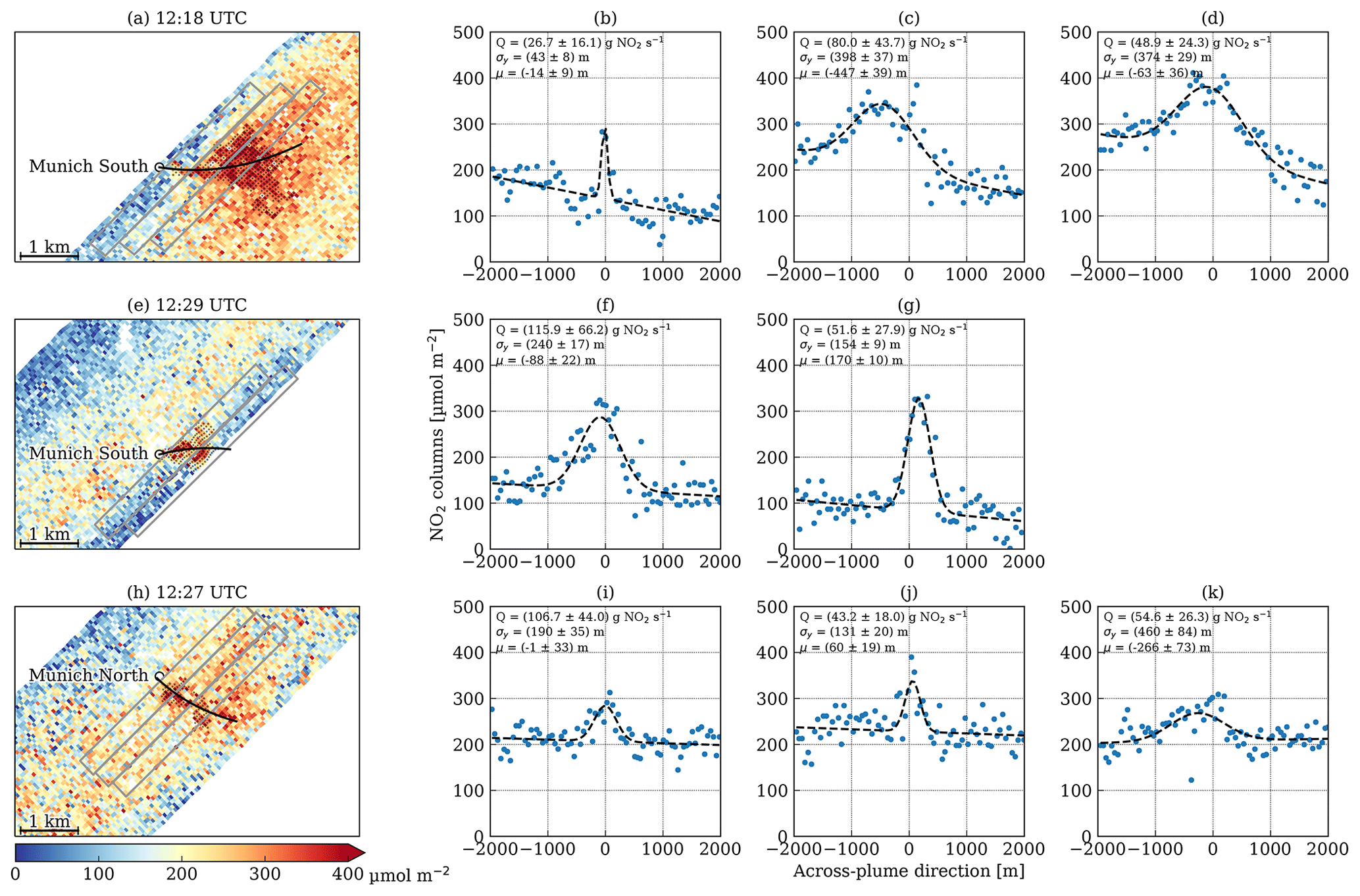
Figure 11 (a, e, h) APEX NO₂ maps with emission plumes (black dots) of the Munich South and Munich North CHP plants. The center line of the plume is shown as a black curve. (b–d, f, g, i–k) APEX NO₂ VCDs averaged in the across-track direction within gray boxes shown in the maps and a Gaussian curve fitted to the observations (dashed line).

3.6 NO_x and CO₂ emissions of point sources

The two largest point sources in the city are the Munich North CHP plant and Munich South CHP plant (see Fig. 1). For 2016, Munich North reported CO₂ and NO_x mean emissions of 80 kg CO₂ s⁻¹ and 53 g NO₂ s⁻¹, respectively, and Munich South reported 26 kg CO₂ s⁻¹ and 14 g NO₂ s⁻¹ (European Environment Agency, 2021). Since instantaneous emissions usually differ from annual means, we calculated the instantaneous emissions of Munich South using the natural gas consumption provided by the operating Stadtwerke München (SWM) using a conversion factor of 1.9225 kg CO₂ per Nm³ natural gas (U.S. EPA, 2016) and the mass ratio of annual CO₂ and NO_x emissions. The computed emissions are 44.2 kg CO₂ s⁻¹ and 23.1 g NO₂ s⁻¹, which is about 70 % higher than annual means, and only vary slightly by ±1.3 kg CO₂ s⁻¹ and ±0.7 g NO₂ s⁻¹ between 09:30 and 14:00 UTC on 7 July 2016.

CO₂ and NO_x emissions can be estimated from CO₂ and NO₂ observations. APEX flew once over Munich North at 12:27 UTC (stripe 2) and twice over Munich South at 12:18 and 12:29 UTC (stripes 1 and 2). The NO₂ emission plumes of the two CHP plants are visible in the APEX observations (Fig. 11a, e, and h). In addition, the CO₂ plume of Munich South was observed by the FTIR spectrometers (Fig. 12).

Figure 12a shows the setup of the two FTIR spectrometers where the instruments can observe XCO₂ upwind and downwind of the plume. The XCO₂ time series of the instruments is shown in Fig. 12c. The KIT instrument frequently observed the CO₂ enhancement of the CHP plant plume downwind of the source, while the TUM instrument observed the upwind values. Since the plume location meanders depending on wind speed and direction, the line of sight of the FTIR instrument will not always include the plume. In fact, during the APEX measurements, the FTIR instruments did not capture any CO₂ enhancements, because the line of sight followed the Sun towards the west while the wind carried the plume towards the southeast. Figure 12b shows the APEX NO₂ field overlaid with the lines of sight of the two FTIR spectrometers, confirming that the plume was not in the instrument's field of view at APEX overpass time.

3.6.1 NO_x emissions

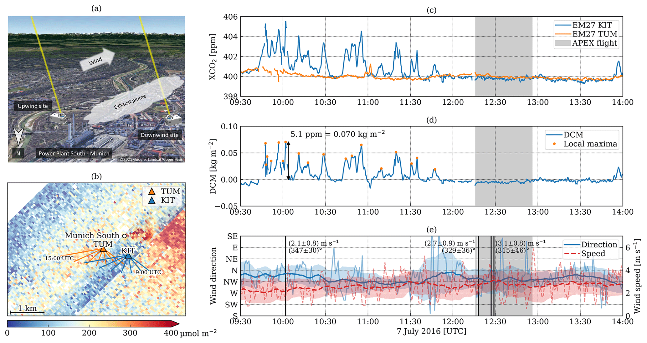
Figure 12 (a) The setup of the two FTIR spectrometers at Munich South. (b) APEX NO₂ map showing the NO₂ emission plume and the locations of the FTIR spectrometers. The lines are hourly lines of sight below 1100 m above ground. (c) XCO₂ time series and (d) differential CO₂ measurements (DCM) for the two instruments. (e) Wind speed and direction measured every minute on the LMU rooftop at 30 m above ground (thin lines). In addition, a 30 min rolling average was applied to the time series (thick lines). The shaded area shows the 1σ temporal variability within 30 min. Vertical lines show times with the largest CO₂ peak and NO₂ measurements by the APEX instrument. The numbers are 30 min mean wind speed and direction.

The NO_x emissions of the Munich North and Munich South CHP plants were estimated from the APEX observations using a plume detection algorithm and mass-balance approach implemented as part of a Python package for “Data-driven Emission Quantification” (Kuhlmann, 2021a; Kuhlmann et al., 2021). The NO_x emissions Q were obtained by computing the cross-sectional flux as

$$\begin{array}{}\text{(5)}& Q=f\left(x\right)\cdot q\left(x\right)\cdot u\left(x\right)\cdot \cos \left(\mathit{\alpha }\left(x\right)\right),\end{array}$$

where x is the along-plume coordinate, f is the NO₂ : NO_x conversion factor, q is the line density, and ucos (α) is the wind speed normal to the cross section used for computing the line density. The line density was computed by fitting a Gaussian curve to the along-track NO₂ VCDs:

$$\begin{array}{}\text{(6)}& \mathrm{VCD}\left(y\right)={\displaystyle \frac{q}{\sqrt{\mathrm{2}\mathit{\pi }}\mathit{\sigma }}}\exp \left(-{\displaystyle \frac{(y-\mathit{\mu }{)}^{\mathrm{2}}}{\mathrm{2}{\mathit{\sigma }}^{\mathrm{2}}}}\right)+my+b,\end{array}$$

where y is the across-plume coordinate, μ is a shift, and σ is the standard width. The NO₂ background was approximated by a linear function with slope m and intercept b.

To compute the across- and along-plume coordinates, the location and extent of the NO₂ emission plumes were determined using a plume detection algorithm, which detects pixels where the local mean is significantly enhanced above the background (Kuhlmann et al., 2019, 2021). The local mean was computed using a Gaussian filter with a standard width of 0.75 pixels. The background was computed as the median of 100 adjacent pixels in the along-track direction to avoid issues with across-track stripes. A 2D curve was then fitted to the detected pixels to describe the center line of the plume. x and y coordinates were computed as arc length from the source and the distance from the curve, respectively. The tangent of the curve was used to determine the wind direction that is used to compute the angle α.

A critical input for estimating the emissions is the wind speed profile, which determines the height of the plume due to plume rise and the wind speed inside the plume. Figure 12e shows the time series of wind speeds and directions measured on the MIM's rooftop at 30 m above ground. The wind speed measured every minute shows high variability with a standard deviation of about 0.9 m s⁻¹ for 30 min rolling means. Since MIM's rooftop is more than 3 km away from the stacks, the highly variable wind measurements are not well suited as input for estimating emissions. We therefore used the simulations from the COSMO-1 and COSMO-7 analysis products. The 10 m wind fields and vertical profiles are shown in Figs. S11 and S12. Since the COSMO-1 model with about 1 km resolution shows small convective cells whose locations are determined by a stochastic process, we average 6×6 grid cells to obtain an average wind profile and its uncertainty at the stack locations.

The plume height needs to consider plume rise that can be computed from heat emissions, wind speed at the stack, and the dispersion category (VDI – Fachbereich Umweltmeteorologie, 1985). The Munich South CHP plant has three stacks (H=90 m), for which we use heat emissions of 70 MW obtained from the operator. The dispersion category was already determined as very unstable (category: V) in Sect. 3.1. The wind speed at the height of the stacks is calculated from the COSMO-1 profiles as 2.5±1.3 m s⁻¹ at 10:00 UTC. The plume height starts at the 90 m stack and rises quickly to a maximum height of 845 m at about 1580 m downstream of the stack (Fig. S13). We use the wind speed taken from the COSMO-1 profiles at the height of the plume to estimate NO_x emissions. The distance from the plume is given by the arc length of the center lines. We assume the same heat emissions and stack height to estimate the plume rise for the Munich North CHP plant.

The NO₂ : NO_x conversion factor f was computed using an NO lifetime of 0.3 h for dispersion category V (VDI – Fachbereich Umweltmeteorologie, 2009, Sect. 10.2) and a residence time, which was computed using the distance from the source to the cross section and the wind speed.

The uncertainties were computed using the uncertainty of the NO₂ VCDs in the Gaussian curve fit and the uncertainty of the wind speed from the spatial standard deviation in the COSMO-1 model. The uncertainty of the wind speed affects the uncertainty directly in Eq. (5) and indirectly due to its impact on the NO₂ : NO_x conversion factor. The uncertainty of the conversion factor is also affected by the uncertainty of the NO lifetime, which is difficult to quantify as it requires, for example, detailed simulations of the NO_x chemistry in the turbulent emission plume. For the sake of simplicity, we assume an uncertainty of 50 % in this study. Since the uncertainty of wind speed dominates the total uncertainty, additional factors were not included in the uncertainty calculations.

Figure 11a, e, and h show the three APEX observations at Munich North and Munich South with the detected pixels (black dots) and center lines. Line densities were computed by averaging five lines in the across-track direction within ±2000 m from the center line indicated by the rectangular boxes in the figure. The input parameters and the estimated NO_x emissions are shown in Table S2. For Munich South, estimated NO_x emissions range from 26.7 to 115.9 g NO₂ s⁻¹, with an average of 64.6±20.3 g NO₂ s⁻¹, i.e., a relative uncertainty of 31 %, where the uncertainty is the standard error of the mean. For Munich North, only three line densities could be computed, resulting in emissions ranging from 43.2 to 106.7 g NO₂ s⁻¹ (average: 68.2±24.8 g NO₂ s⁻¹).

3.6.2 CO₂ emissions

The CO₂ emission strength can be estimated from the differential column measurements (DCMs), i.e., the difference between the upstream and downstream observations, which represents the enhancement due to the source (Fig. 12a, Chen et al., 2017). If we assume that the emission plume can be approximated by a Gaussian plume model and that the local peaks in the DCM time series occur when the plume center moves over the downwind station (i.e., they correspond to the maxima in the Gaussian), the source strength Q would be given by

$$\begin{array}{}\text{(7)}& Q=\sqrt{\mathrm{2}\mathit{\pi }}u\left(x\right){\mathit{\sigma }}_y\left(x\right){\mathrm{DCM}}_{\max }\left(x\right),\end{array}$$

where u is the wind speed inside the plume, σ_y is the horizontal width of the plume, and DCM_max is the CO₂ enhancement in the center of the Gaussian plume. Note that u, σ_y, and DCM_max depend on the distance from the source x.

Figure 12d shows the time series of DCMs measured on 7 July 2016. In total, we identified 18 local maxima using a standard peak finding algorithm of the SciPy library (Virtanen et al., 2020, Version 1.4.1) for estimating CO₂ emissions. The highest DCM was measured at 10:02 UTC with 5.1 ppm, which is converted to a mass column density of 0.070 kgm⁻².

The wind speed was taken from the COSMO-1 profiles to compute plume rise and the distance of the plume from the stack at the slant line of sight of the FTIR instrument (Fig. S13). The KIT EM27 spectrometer was located 582 m downstream of the stack. At 10:02 UTC, the line of sight of the instrument and the plume height intersect at a height of 615${}_{-\mathrm{177}}^{+\mathrm{274}}$ m. Consequently, the distance from the source x is 915${}_{-\mathrm{114}}^{+\mathrm{485}}$ m downstream of the source. The dispersion coefficients were computed based on VDI guidelines, which assumes constant coefficients above 180 m. It is computed by an empirical equation ${\mathit{\sigma }}_y\left(x\right)=F\cdot x^f$ with F=0.671 and f=0.903 for dispersion category V. Therefore, σ_y(x) ranges were computed as 317${}_{-\mathrm{36}}^{+\mathrm{85}}$ m at the intersection. The standard deviations were computed from the spatial variability in COSMO-1 wind speeds.

The CO₂ emissions were then computed by Eq. (7) using a wind speed in the plume center of 2.4±0.7 at 615 m above ground, which results in emissions of 134±49 kg CO₂ s⁻¹. The uncertainty was estimated using a DCM uncertainty of 0.1 ppm for 1 min averages (Chen et al., 2016) as well as the uncertainties of u(x) and σ_y(x). The uncertainty budget is dominated by the uncertainty in the wind speed that accounts for 72 % of the total uncertainty. The uncertainty of the dispersion coefficient σ_y accounts for 27 % of the total uncertainty, which also depends on the uncertainty of the wind speed, while the uncertainty of the DCM measurements is negligible.

The emissions were computed for all 18 peaks, and results are shown in Table S3. The estimated CO₂ emissions vary strongly, ranging from 38 to 134 kg CO₂ s⁻¹. The mean and standard error of all 18 estimates are 81.2±8.6 kg CO₂ s⁻¹.

3.6.3 Comparison with reported emissions

CO₂ and NO_x emissions of the Munich South CHP plant were estimated as 81.2±8.6 kg CO₂ s⁻¹ and 64.6±20.3 g NO₂ s⁻¹, significantly higher than the emissions of 44.2±1.3 kg CO₂ s⁻¹ and 23.1±0.7 g NO₂ s⁻¹ computed from fuel consumption. The NO_x-to-CO₂ emission ratios are similar between reported and estimated emissions.

The main reason that the estimated emissions are higher than the reported values is likely due to the unstable and highly turbulent atmospheric boundary layer resulting in low and highly variable wind speeds, which makes applying mass-balance approaches challenging for estimating emissions. On the one hand, uncertainties are large, because accurate knowledge of the wind speed is critical, as it not only affects the computation of the flux, but also the calculation of plume rise, dispersion coefficient, and NO lifetime. On the other hand, mass-balance approaches assume stationary conditions, which is not very accurate, especially in turbulent flow conditions.

The method applied to estimating CO₂ emissions from the FTIR measurements assumed that the plume can be approximated by a Gaussian plume model and that the local maxima are the maxima in the vertically integrated Gaussian plume. However, maxima in the time series also occur when the wind speed is below the average. As a result, the assumption of an average wind speed would overestimate the CO₂ emissions. The individual COSMO-1 wind profiles (Fig. S12) show that the lower wind speeds would halve the values, which would also lead to a halving of estimated CO₂ emissions much more consistent with our estimate from fuel consumption. The turbulent flow will also result in puff-like structures in the plume, where CO₂ values are locally enhanced or reduced compared to a Gaussian model, which will either overestimate or underestimate emissions. Furthermore, it is possible that only the edge of the plume passes briefly through the line of sight, which would result in a local maximum but underestimate the emissions. To limit the impact on our estimate, we have estimated emissions for all local peaks in the time series, yet our estimates are still likely to be too high, as the algorithm for identifying peaks does not account for minor peaks.

The computation of the cross-sectional flux for estimating NO_x emissions from the APEX NO₂ observations is also limited by the turbulent flow, because the emission plumes are already very wide just 1 km downstream of the source, which makes it difficult to determine the center line of the plume and the angle between APEX stripe and wind vector. The wind profiles from the simulations and the measurements are less consistent in the afternoon, and the COSMO-1 wind profiles might be overestimated (Fig. S12), which could explain the overestimated NO_x emissions. In addition, the estimation of NO_x emissions is sensitive to the NO₂-to-NO_x conversion factor f, which in turn depends on NO lifetime and wind speed. For turbulent flow, the residence time is likely longer than the value computed from mean wind speed and distance from the source, resulting in a smaller conversion factor and consequently lower estimated NO_x emissions. Finally, it should also be noted that NO lifetime given by the VDI guidelines might not be sufficiently accurate for conditions on the campaign day.

4 Conclusions

In this paper, we presented results from the MuNIC measurement campaign conducted in July 2016 in Munich. The campaign measured NO₂ near-surface concentrations (NSCs) and vertical column densities (VCDs) with stationary, mobile, and airborne in situ and remote sensing instruments. A central element of the campaign was a measurement flight with the APEX imaging spectrometer mapping the spatial distribution of NO₂ VCDs on the afternoon of 7 July 2016.

Our results confirm that airborne imaging remote sensing is suited for spatial mapping of NO₂ VCDs and the detection of emission plumes from larger point sources and cities. The obtained NO₂ VCD retrievals have a moderate correlation with mobile MAX-DOAS measurements conducted on the same afternoon (r=0.55), and estimated uncertainties are similar to previous findings (e.g., Tack et al., 2017). The NO₂ map obtained from the APEX data could depict the coarse-scale NO₂ distribution with lower values upwind and higher values downwind of the city but with no strong signatures of individual sources except for the two power plants.

We observed substantial differences between VCDs and NSCs. While APEX NO₂ VCDs are not elevated along roads, NSCs show high spatial and temporal variability along roads, with the highest values in congested areas and tunnels. One reason for these differences is atmospheric mixing, but 3D radiative transfer effects were also recently found to reduce the effective spatial resolution of the ground pixels and cause random uncertainties in the presence of buildings as well as an underestimation of NO₂ VCDs due to building shadows (Schwaerzel et al., 2021).

The transfer function t required for converting VCDs to NSCs is important when using imaging remote sensing for air pollution studies. However, a constant transfer parameter, calculated as the ratio of NSC over VCD from the observations, results in a very high RMSE when NSCs would be computed from VCDs. More advanced methods (than a simple constant factor) need to be applied to convert airborne NO₂ maps to near-surface concentrations. A way forward could be to combine airborne observations with a city-scale dispersion model that links NSCs and SCDs and that also needs to consider 3D radiative transfer. The unique dataset collected in the MuNIC campaign will be important for validating such approaches.

We found that NO_x emission estimates of the two combined heat and power (CHP) plants are significantly higher than reported values, but uncertainties are high due to high variability in wind speeds during the campaign day. Wind speeds are required to compute the fluxes as well as plume rise, dispersion, and residence time that have a large impact on the estimated emissions. The estimates are also likely overestimated, because the applied mass-balance approaches assume steady-state conditions, which seems to be insufficient for convective conditions if accurate and high-resolution wind fields are not available. Nonetheless, NO_x emission estimates for Munich South are consistent with CO₂ emissions determined from two ground-based FTIR instruments.

Due to the difficulty in estimating emission from airborne imaging spectrometers under convective conditions, flying during stable conditions, i.e., higher and less variable wind speeds and directions, should be an option to reduce uncertainties in future campaigns. While conditions tend to be less convective in the early morning and late afternoon, such conditions increase other challenges, including large solar zenith angles, for which 3D radiative transfer effects can affect emission estimates (Schwaerzel et al., 2020). For the planning of future campaigns, it is therefore important to consider both illumination and wind conditions in order to obtain the best possible situation for measurements and data analyses.