the Creative Commons Attribution 4.0 License.
the Creative Commons Attribution 4.0 License.
 | 21 Mar 2022
IRIS analyser assessment reveals sub-hourly variability of isotope ratios in carbon dioxide at Baring Head, New Zealand's atmospheric observatory in the Southern Ocean
Gordon W. Brailsford
Rowena C. Moss
John McGregor
Ross J. Martin
Sylvia Nichol
Sara Mikaloff-Fletcher
Beata Bukosa
Magda Mandic
C. Ian Schipper
Paul Krummel
Alan D. Griffiths
We assess the performance of an isotope ratio infrared spectrometer (IRIS) to measure carbon (δ13C) and oxygen (δ18O) isotope ratios in atmospheric carbon dioxide (CO2) and report observations from a 26 d field deployment trial at Baring Head, New Zealand, NIWA's atmospheric observatory for Southern Ocean baseline air. Our study describes an operational method to improve the performance in comparison to previous publications on this analytical instrument. By using a calibration technique that reflected the principle of identical treatment of sample and reference gases, we achieved a reproducibility of 0.07 ‰ for δ13C-CO2 and 0.06 ‰ for δ18O-CO2 over multiple days. This performance is within the extended compatibility goal of 0.1 ‰ for both δ13C-CO2 and δ18O-CO2, which was recommended by the World Meteorological Organization (WMO). Further improvement in measurement performance is desirable to also meet the WMO network compatibility goals of 0.01 ‰ for δ13C-CO2 and 0.05 ‰ for δ18O-CO2, which is needed to resolve the small variability that is typical for background air observatories such as Baring Head.
One objective of this study was to assess the capabilities and limitations of the IRIS analyser to resolve δ13C-CO2 and δ18O-CO2 variations under field conditions. Therefore, we selected multiple events within the 26 d record for Keeling plot analysis. This resolved the isotopic composition of endmembers with an uncertainty of ≤ 1 ‰ when the magnitude of CO2 signals is larger than 10 ppm. The uncertainty of the Keeling plot analysis strongly increased for smaller CO2 events (2–7 ppm), where the instrument performance is the limiting factor and may only allow for the distinction between very different endmembers, such as the role of terrestrial versus oceanic carbon cycle processes.
- Article
(5398 KB) - Full-text XML
- BibTeX
- EndNote


Carbon dioxide (CO2) is the single most important anthropogenic greenhouse gas, and it is therefore of critical importance to understand biogeochemical processes controlling atmospheric CO2 levels (IPCC, 2021). The isotopic composition of atmospheric CO2 at any time and location is controlled by different carbon cycle processes and can therefore be used to constrain carbon fluxes on a range of spatio-temporal scales. For example, Ciais et al. (1995a, b) have used stable carbon isotope ratio in atmospheric CO2 (δ13C-CO2) in weekly samples from 43 sites to distinguish terrestrial and ocean sink fluxes. Keeling et al. (2017) also used δ13C-CO2 from flask samples to infer changes in water use efficiency of plants with increasing atmospheric CO2 mole fractions. Similarly, the oxygen isotope ratios in CO2 (δ18O-CO2) have been used as a tracer for gross primary production (GPP) of the terrestrial biosphere (Francey and Tans, 1987; Ciais et al., 1997). Using global δ18O-CO2 records, Welp et al. (2011) demonstrated the impact of El Niño–Southern Oscillation on the global carbon cycle and provided revised GPP estimates that exceeded previous values by ∼ 30 %, due to shorter cycling time of CO2. Much of the knowledge on isotope ratios in atmospheric CO2 has been generated by isotope ratio mass spectrometry (IRMS) measurements in discrete air samples (Ferretti et al., 2000; Werner et al., 2001; Allison and Francey, 2007; Brand et al., 2016), often requiring a complex and well-operated logistical network (Ciais et al., 1995a; Welp et al., 2011; Keeling et al., 2017). This may be particularly challenging for tracers such as δ18O-CO2, which can be subject to storage effects in flasks (Rothe et al., 2005; Vardag et al., 2015). In order to provide guidance to instrument manufacturers and laboratories, the World Meteorological Organization (WMO) recommends compatibility goals for atmospheric observations, including δ13C-CO2 and δ18O-CO2. Instruments meeting the ambitious network compatibility goals (0.01 ‰ for δ13C-CO2 and 0.05 ‰ for δ18O-CO2) are considered capable of resolving very small atmospheric signals typical for baseline air in remote locations, while those meeting the more relaxed extended compatibility goals (0.1 ‰ for both δ13C-CO2 and δ18O-CO2) can be expected to resolve larger signals typically observed in regional or urban studies (WMO-GAW, 2019).
The potential for field-deployable, laser-based instruments measuring both mole fractions and isotope ratios in atmospheric CO2 in real time has been demonstrated (Bowling et al., 2003; Mohn et al., 2007). Continuous technical improvement of both analysers and applied calibration techniques enables an achievable measurement precision that is increasingly comparable to that of well-performing IRMS systems (Tuzson et al., 2011; Griffith et al., 2012; Sturm et al., 2013; Hammer et al., 2013; Flores et al., 2017; Pieber et al., 2021) and is approaching the compatibility goal of the WMO (Steur et al., 2021). With that, laser-based instruments may be an interesting alternative for observations that were previously limited to IRMS laboratories and flask sampling programmes. The performance of these techniques was demonstrated in the monitoring of annual and seasonal cycles with high temporal resolution (Sturm et al., 2013; Vardag et al., 2016; Pieber et al., 2021). Moreover, real-time measurements of CO2 and its stable isotopes open new research opportunities that researchers have hitherto not been able to explore. For example, the high temporal resolution achievable with laser-based instruments enables observations ranging from synoptic scales (Vardag et al., 2015, 2016; Pieber et al., 2021) to that of micrometeorological observations (Griffis et al., 2008; Wehr et al., 2013), for which IRMS-based techniques are not a feasible long-term solution.
Commercially available instruments show a large variability in their performance (i.e. achievable measurement precision) and in the level of operator knowledge and interaction required to make meaningful measurements. Key questions address (i) how the achievable instrument performance of field-deployed instruments compares to traditional IRMS techniques and other laser-based instruments and (ii) what new research opportunities these techniques may provide.
In this study, we assess the performance of an IRIS analyser, the Delta Ray, previously manufactured by Thermo (Thermo Fisher Scientific, Bremen, Germany). Note that Thermo has discontinued the manufacturing of the Delta Ray since the experiments of this study were completed. The first studies that deployed the then new Delta Ray instrument in the field have demonstrated its capability to resolve large variations in both CO2 mole fractions (up to 100 ppm) and isotope ratios (up to 15 ‰). These studies included CO2 observations (i) at carbon storage and sequestration sites (Van Geldern et al., 2014), (ii) of volcanic CO2 emissions (Rizzo et al., 2014; Schipper et al., 2017), (iii) at a forest site (Braden-Behrens et al., 2017) and (iv) in a cave system (Töchterle et al., 2017). Both Van Geldern et al. (2014) and Braden-Behrens et al. (2017) report Allan deviation minima for δ13C-CO2 of around 0.04 and 0.02 ‰, respectively. However, both publications also report final measurement uncertainties of their field-deployed instruments of 0.3 ‰. Töchterle et al. (2017) and Flores et al. (2017) report uncertainties of 0.34 ‰ and 0.18 ‰ for δ13C-CO2 and 0.44 ‰ and 0.48 ‰ for δ18O-CO2, respectively. Only Rizzo et al. (2014) reports a precision that is close to the values of reported Allan deviations with < 0.05 ‰. Altogether, these studies reveal a significant difference between Allan deviation and the reported measurement uncertainties, suggesting that the latter may be improved significantly. Achieving uncertainties closer to the compatibility goals of the WMO (WMO-GAW, 2019) potentially increases the variety of research questions this instrument may help to answer.
We tested the Delta Ray instrument in our laboratory and at Baring Head (BHD), our observatory for Southern Ocean background air (Brailsford et al., 2012). Generally, Southern Ocean background air shows very little variability in CO2 mole fractions (Stephens et al., 2013; Steinkamp et al., 2017) and isotope ratios (Allison and Francey, 2007; Moss et al., 2018), providing one of the most challenging environments to explore the performance of a field-deployed instrument for such measurements (Pieber et al., 2021). We compare Delta Ray data with co-located observations of CO2 mole fractions in the context of meteorology and the variability of radon. Due to the unfortunate failure of the automated air sampler at BHD during the time of the Delta Ray deployment, we cannot provide a direct comparison of the Delta Ray and our well-established gas chromatography isotope ratio mass spectrometer (GC-IRMS) system (Ferretti et al., 2000; Moss et al., 2018). However, we compare the Delta Ray data from background air events with interpolated δ13C-CO2 and δ18O-CO2 observations from BHD and the Cape Grim Observatory (CGO). Despite the limitation to resolve the isotope variability of the smallest CO2 signals (i.e. CO2 variability ≤ 2 ppm), the Delta Ray time series provides valuable information on the processes controlling the variability of CO2 at BHD on synoptic and daily timescales.
We tested the Delta Ray instrument in two separate campaigns. An early Delta Ray model was used during 2015 in NIWA's atmospheric laboratory for Allan deviation and stability tests, as well as during the deployment at the BHD observatory. In 2018, we used a factory-refurbished Delta Ray model with improved precision. This instrument was used for CO2-free air experiments before it developed faulty behaviour and had to be returned to Thermo without deployment at BHD.
2.1 The Delta Ray analyser
The physical principle of the Delta Ray has been described in detail in previous publications (Van Geldern et al., 2014; Töchterle et al., 2017; Braden-Behrens et al., 2017). In short, the instrument measures the absorption spectrum of CO2 in the mid-infrared range. It comprises of two units, the analyser and the universal reference interface (URI). The URI dilutes isotopically known, pure CO2 gases with CO2-free air and supplies this mixture as reference gas to the laser unit. The operating software (Qtegra) controls the CO2 mole fraction in the reference gas by matching the average mole fraction of a previously measured sample. This concept is applied to account for the CO2 amount effect on the measured isotopic composition of the analyser (Braden-Behrens et al., 2017). The software calculates the isotopic composition of the unknown samples using the isotope values of the two pure CO2 gases. This two-point calibration also accounts for the so-called “scale compression”. Furthermore, the system requires an air standard with known CO2 mole fractions to calibrate the mole fraction measurements of the Delta Ray. Once all gases are connected and the operating temperature has stabilised, the instrument requires a calibration procedure to determine factors for linearity, scale compression, isotope calibration, mole fraction calibration and for the mass flow controller that mixes pure CO2 with the carrier gas. Qtegra applies these factors to all following sample measurements. Thermo specifies the achievable instrument precision to be 0.07 ppm for CO2 mole fractions and as low as 0.05 ‰ for both δ13C-CO2 and δ18O-CO2 (Thermo, 2014).
2.2 Reference gases, quality-control gases and carrier gases
Two electropolished 1 L stainless-steel flasks were filled to 5 bar with two pure, isotopically distinct CO2 gases, referred to as Marsden and Kapuni. We determined δ13C-CO2 and δ18O-CO2 values of −32.77 ‰ and of −32.52 ‰ for Marsden, as well as of −13.75 ‰ and of −11.69 ‰ for Kapuni, respectively (Table 1), using a dual-inlet IRMS system and VPDB scale realisation described by Lowe et al. (1994). Over all experiments, we re-filled the flasks with Marsden and Kapuni following the same filling protocol but did not re-calibrate the aliquots. Thereby, we assign a conservative uncertainty of 0.1 ‰ to the isotope values used for both gases (Table 1). While the isotopic difference between Marsden and Kapuni is in the range of the reference gases that Thermo supplies commercially for that purpose (“Ambient” and “Bio”), typical values of atmospheric CO2 are outside the range covered by our two gases. Due to its isotopic proximity to that of atmospheric CO2, we used Kapuni as the regularly used reference gas (Ref-1) during all measurements, while Marsden was only used during the initial instrument calibration (Ref-2).
Table 1Two pure CO2 gases used as reference gases (Marsden, Kapuni) were calibrated to VPDB realisation of Lowe et al. (1994). QC-1 served as air standard and QC-2 and QC-3 as target gases, while QC-4 and QC-5 were used during laboratory tests. Mole fractions and isotope ratios are provided with the 1σ uncertainty of their measurement.
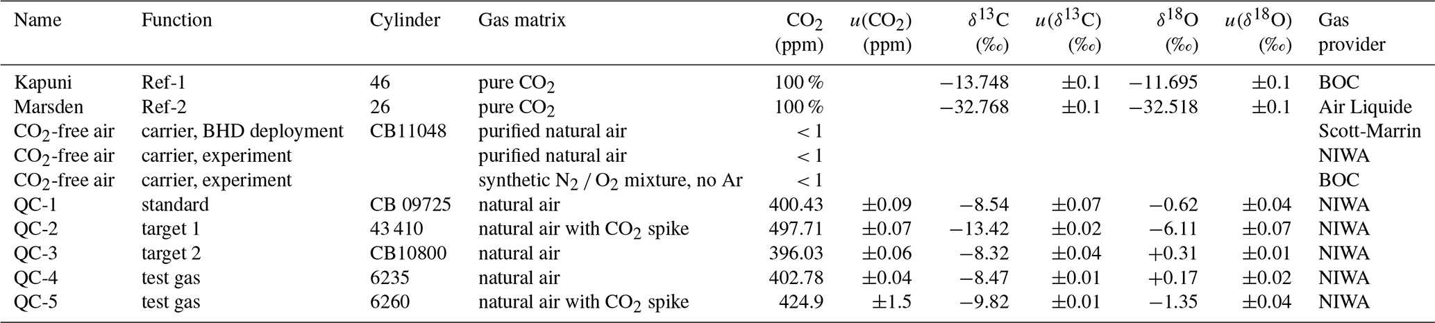
We used a CO2-free air from Scott-Marrin (Scott-Marrin, California, USA, now Linde Gas & Equipment Inc., PA, USA) as carrier gas in the 2015 campaign. Scott-Marrin produces their CO2-free air by purifying natural air (Scott-Marrin, Lori Thomas, personal communication, via email on 16 August 2014) and certifies the CO2-free air with < 1 ppm CO2, which exceeded the recommended level of < 0.5 ppm (Thermo, 2014). To test the effect of different carrier gases on the measured isotopic compositions, we applied a range of CO2-free gases in the 2018 campaign (Sect. 3).
As calibration gas for CO2 mole fractions, we used a 30 L Luxfer cylinder (Scott-Marrin, California, USA, now Linde Gas & Equipment Inc., PA, USA) with compressed natural air, taken at BHD. The CO2 mole fraction was determined by gas chromatography (GC) at NIWA's atmospheric laboratory.
Furthermore, we used five 30 L Luxfer cylinders with compressed air as quality-control gases (referred to as QC-1 to QC-5). The δ13C-CO2 and δ18O-CO2 isotope ratios of the QC gases were measured on NIWA's gas chromatography isotope ratio mass spectrometer (GC-IRMS) system (Ferretti et al., 2000; Moss et al., 2018), using a custom-made peripheral on a MAT252 isotope ratio mass spectrometer (Thermo Finnigan, Germany). The instrument is calibrated using a propagated VPDB-CO2 scale realisation from the Commonwealth Scientific and Industrial Research Organisation (CSIRO, Aspendale, Australia). Two QC gases were included in each measurement cycle. CO2 mole fractions in QC-1 to QC-3 were determined using a gas chromatograph system at NIWA's gas lab, while mole fractions of QC-4 were measured using the Picarro system at BHD (model G2401, Picarro Inc., California, USA) and of QC-5 via comparison of peak sizes on the GC-IRMS instrument, respectively. CO2 mole fractions in QC-1 to QC-4 are calibrated to the WMO CO2 X2007 scale.
2.3 Calibration scheme
Thermo designed an integrated referencing technique for the Delta Ray, in which two pure CO2 gases with known isotopic composition get diluted with CO2-free air to match CO2 mole fraction range of measured air samples. Therein, the system attempts to conserve the isotopic composition of the pure CO2 during the dilution process and to provide a CO2-in-air reference gas to the analyser that has constant isotope ratios at dynamic CO2 mole fractions. The main purpose for this technique is to account for non-linear, CO2-mole-fraction-dependent isotope effects (Thermo, 2014).
However, the application of this compulsory referencing technique does not follow the principle of identical treatment (Werner and Brand, 2001), hereafter referred to as PIT, which is regarded as the golden rule for isotope referencing in the IRMS community. Therefore, we treat the data output of the Delta Ray as preliminary. We designed our measurement sequences to include two quality-control gases (QC-1, QC-2, QC-3) and used QC-1 as the working standard to reference the Delta Ray data to the VPDB isotope scale (Table 1), which followed the PIT and improved the reproducibility of QC-2 and QC-3 significantly.
2.4 Configuration of analytical setup and measurement sequence
The Delta Ray system configuration comprised of the Delta Ray analyser, two pure CO2 gases (Kapuni and Marsden), one CO2-free air as carrier gas, one air standard for CO2 mole fractions and two QC gases at a time (Fig. 1). Kapuni and Marsden are configured in the Qtegra as Reference-1 and Reference-2 (Ref-1 and Ref-2), respectively. The Delta Ray analyser includes an inbuilt Nafion system (Nafion, Perma Pure, USA). However, because this inbuilt Nafion combines the air intake and air outlet in counterflow without water removal, its efficacy is not clear to us, as it potentially mediates water in both directions. Therefore, we used an additional Nafion membrane to dry the incoming air, where the outgoing air was dried using a molecular sieve trap before it was used as drying air in the Nafion membrane. Three-way solenoid valves were used to switch between air samples and QC gases. The valves were configured so that air samples were measured in the normally closed position, to ensure the QC gas cylinders were closed during potential electric failure. Air samples and QC gases were introduced via sample port B, to fulfil the PIT as much as possible.
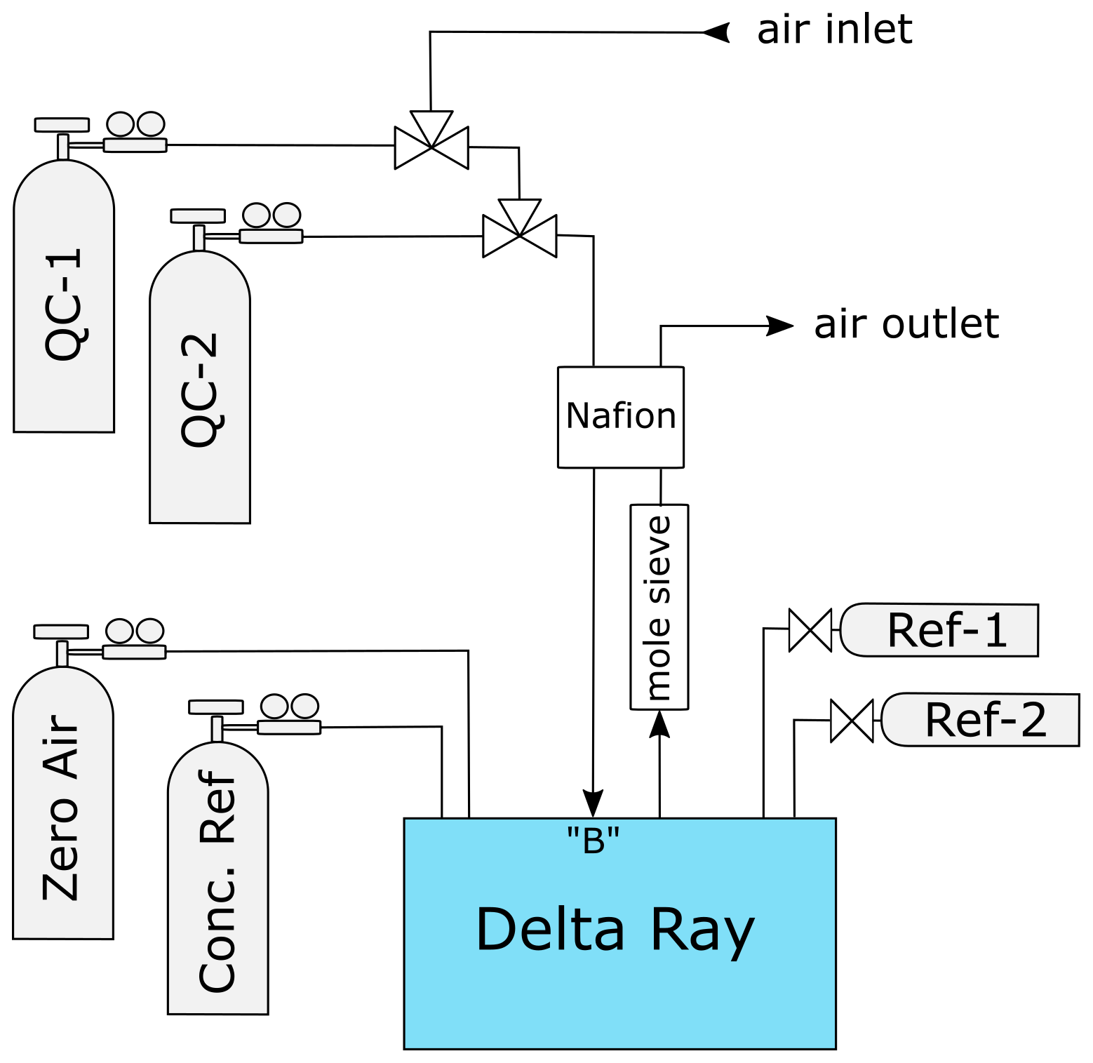
Table 2Timing used for blocks in measurement sequence, resulting gas consumptions, resulting requirements for cylinder replacements per year and relative time each gas was measured.
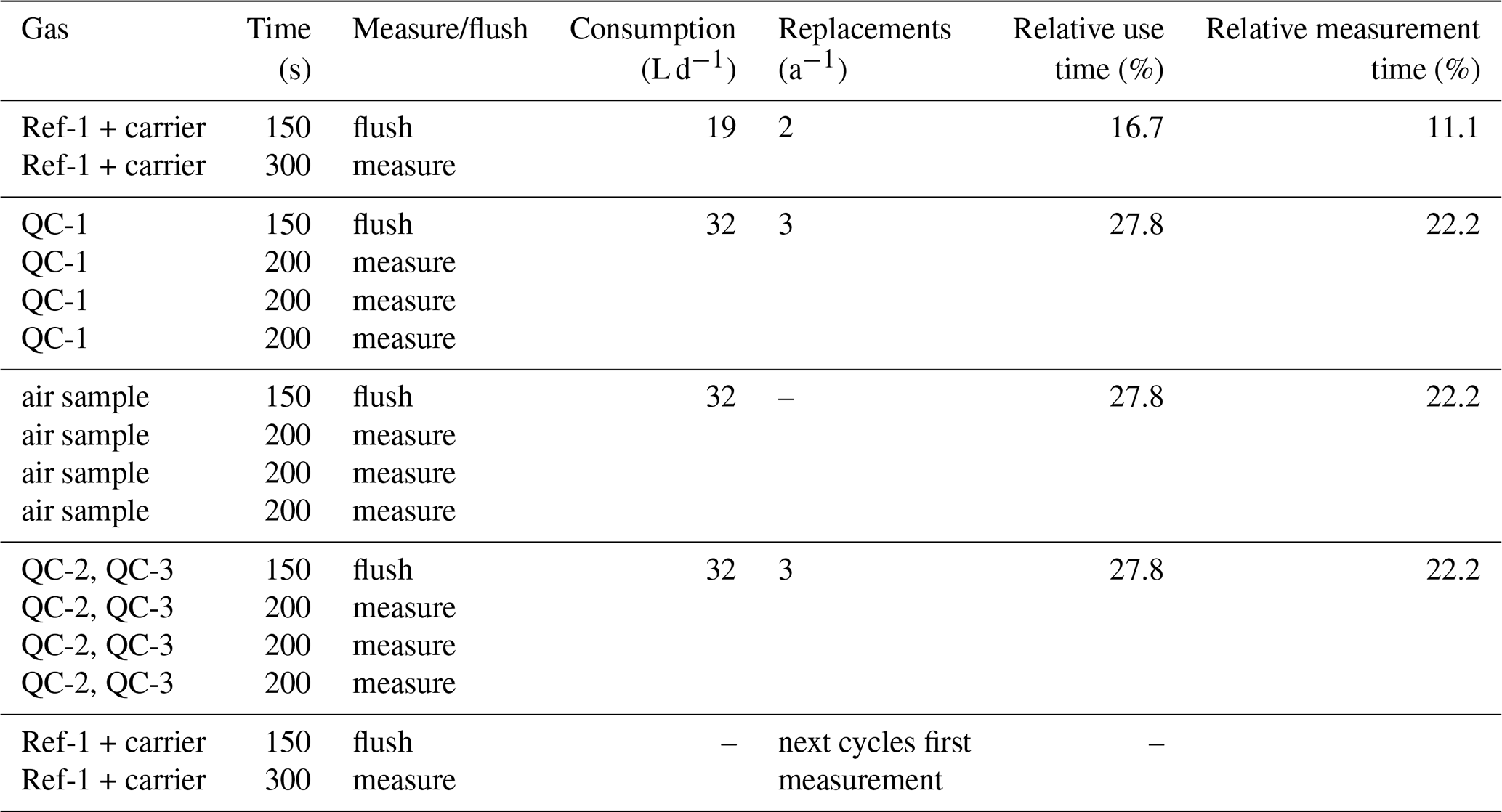
The Delta Ray has the capability to control up to four external solenoid valves, and we used two of these to switch between ambient air and the two QC gases. Measurement sequences were defined in Qtegra and executed in continuous cycles (Table 2). Each measurement sequence begins with the measurement of Ref-1, which is followed by measurement blocks of QC-1, air sample and QC-2, before another Ref-1 measurement block marks both the end of the current measurement sequence and the start of the next measurement sequence. The time resolution of the instrument is 1 Hz. We allowed a flush time of 150 s after each gas change, to ensure complete gas replacement in the inlet lines and the optical cell. This was determined by the time it took for stabilisation after switching between two cylinders, plus generous allowance of additional time, with the goal to prevent the need for future adjustments of the measurement sequence. While the flush time could have been optimised further, this was regarded as low priority. Thereafter, Ref-1 was measured for 300 s, while air and QC gases were measured in three blocks of 200 s each, leading to a total time of 45 min per measurement sequence. This measurement sequence resulted in only 10 min of effective air measurement in every 45 min. Because the objective of this test was to assess the analyser performance, our sequence included a disproportional amount of QC gas measurements. For the data analysis, we calculated average values of each measurement block, resulting in ∼ 32 data points for air and QC gases per 24 h period.
Considering the gas flow rate of 80 mL min−1 through the analyser, as well as the measurement and flush times we defined for reference and QC gases in the measurement sequence, the Delta Ray consumed 19 L of CO2-free air and 32 L of each of the two QC gases per day. In this configuration, cylinders with 30 L volume filled to 138 bar (2000 PSI) would be exhausted in 215 d for CO2-free air and in 129 d for QC gases. This would require two to three cylinder replacements per year (Table 2). The QC gas consumption would decrease significantly with greater proportion of air measurements. However, Thermo recommends a frequency of Ref-1 measurements of 1 per 30 min, which means the CO2-free air consumption should not be decreased further.
2.5 Data correction and uncertainty propagation with QC-1
QC-1 was selected as the working standard to convert all mole fraction and isotope ratio measurements to the respective scales (Table 1). QC-1 comprised of natural air with similar mole fractions and isotope ratios of CO2 to the air measured during the campaign to fulfil the PIT.
Table 3Target values (GC and GC-IRMS) and Delta Ray measurements for QC-1, QC-2 and QC-3 as determined during operation at BHD and differences as Delta Ray minus GC-IRMS and values for QC-2 after correction for the offset in QC-1 minus the GC-IRMS target value.
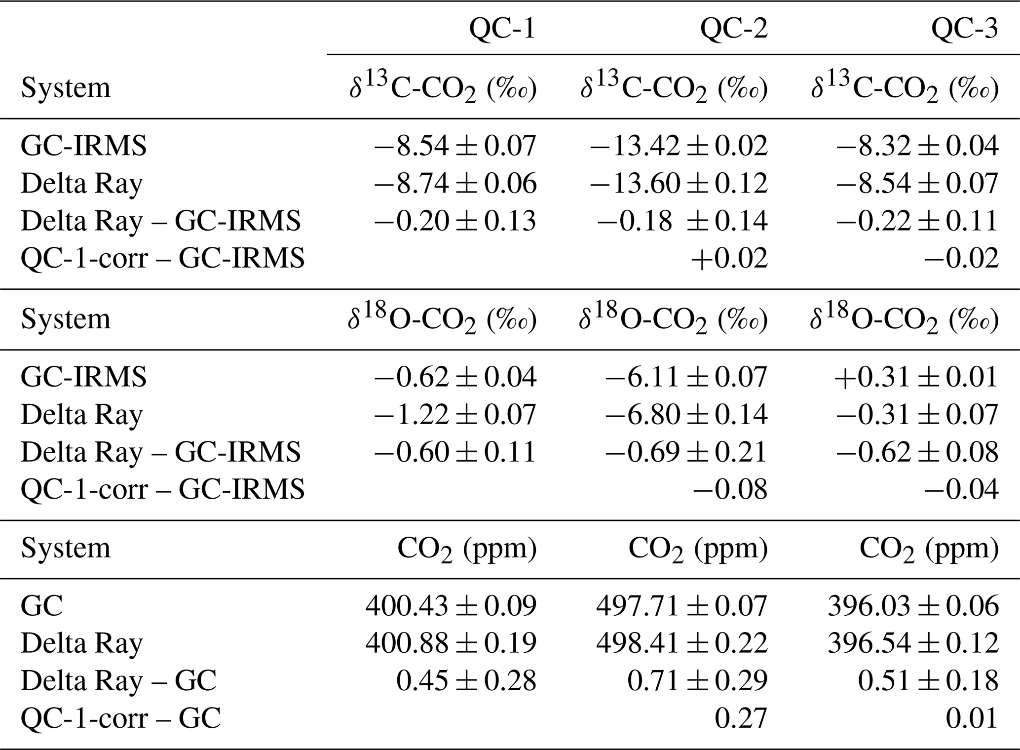
From unprocessed data, we derived average values for δ13C-CO2, δ18O-CO2 and CO2 in QC-1 of −8.74 ± 0.06 ‰, −1.22 ± 0.07 ‰ and 400.88 ± 0.19 ppm, respectively. The comparison to the calibrated values (Table 1) suggests that the long-term averages of the Delta Ray measurements in QC-1 are too depleted in both 13C and 18O by −0.20 ± 0.13 ‰ and −0.60 ± 0.11 ‰, respectively, while they are too high in CO2 by 0.45 ± 0.28 ppm (Table 3). The magnitude of this offset is consistent for QC-2 and QC-3, suggesting a correction for the offset in QC-1 is suitable for all measured parameters in all gases. We correct all Delta Ray measurements according to
where Xs(n) is the calibrated sample average as measured in sequence n on the respective scale, XDR-s(n) and XDR-QC1(n) are the measurement averages for the sample and QC-1 within measurements sequence n, and Xscale-QC1 refers to the calibrated value for QC-1 (Table 1).
Likewise, we calculated the uncertainty of Xs(n) as
where Us(n) is the fully propagated uncertainty of each sample in measurement sequence n, while UDR-s(n) and UDR-QC1(n) are the standard deviations of the Delta Ray measurements for sample and QC-1 in measurement sequence n, respectively (Sect. 2.4). Uscale-QC1 refers to the uncertainty of the target value assignment of QC-1 (Table 1). This correction and uncertainty propagation is applied to all δ13C-CO2, δ18O-CO2 and CO2 measurements in air, QC-2 and QC-3.
3.1 Quality requirements for CO2-free air as carrier gas
Optical analysers for measurements of air samples, such as the Delta Ray, are sensitive to changes in the composition of the air matrix, i.e. the mole fractions of N2, O2 and Ar (Werle et al., 1993; Chen et al., 2010; Thermo, 2014), referred to as the pressure-broadening effect. To prevent the pressure-broadening effect, it is of paramount importance that the air matrix in air samples and reference gases is identical, following the PIT. For measurements of natural air samples with the Delta Ray, the CO2-free air used as carrier gas must therefore comprise of a natural, ultra-pure air matrix (N2 = 78 %, O2 = 21 %, Ar = 1 %) and have a CO2 blank of < 0.5 ppm (Thermo, 2014).
The calibration strategy of the Delta Ray setup as recommended by Thermo is largely dependent on the quality of the CO2-free air, where CO2-free air of sub-optimal quality may limit the achievable accuracy of the system. Because of that, Delta Ray users need to manage their long-term CO2-free air requirements in addition to their reference gas usage. For example, research applications such as long-term atmospheric monitoring with measurement focus on very small signals also require the lowest possible variability in both air matrixes and CO2 blanks between consecutive CO2-free air cylinders. The setup we built for this study uses Ref-1 as mediator only. The final referencing of air measurements is based on QC-1, which fulfils the PIT and therefore mitigates potential variability due to variation in the quality of consecutive CO2-free air supply.
3.2 CO2-free air mixed from pure N2 and O2
Commercial CO2-free air can be manufactured by mixing main air components of high purity, such as the ultra-zero-grade air from BOC (BOC, Linde Group, Wellington, New Zealand) with CO2 ≤ 1 ppm, O2 = 21 ± 1 % and Ar = 0 %, in N2 balance. Ultra-zero-grade air is the highest-quality zero air product that is readily available in New Zealand; however, its certified values neither satisfy the quality criteria for the remaining CO2 level nor for the composition of the matrix air. This highlights potential logistical limitations to source suitable CO2-free air from local gas providers. We attempt to quantify the consequences that can be expected when the CO2-free air is not meeting requirements. Because instruments in our laboratory are not calibrated for sub-ppm measurements of CO2 mole fractions, we introduce the CO2-free gases into the Delta Ray and measure the transmission in the absorption spectra to get a quantitative estimate of the CO2 blank (Fig. 2). With a certified CO2 blank of ≤ 1 ppm, the ultra-zero-grade air from BOC resulted in a transmission of 0.7 % on the main peak of the main isotopologue (indicated as 626 for 16O12C16O). Passing the ultra-zero-grade air through a chemical CO2 scrubber (Carbosorb, Elemental Microanalysis, Devon, UK) reduced the transmission to 0.2 %. By comparing the two transmission values, we think that it is likely that the chemical scrubbing reduced the CO2 blank to ≤ 0.5 ppm and thus meets the manufacturer's CO2-blank requirements. Further CO2 removal from commercial carrier gases may be required to achieve acceptable CO2 levels.
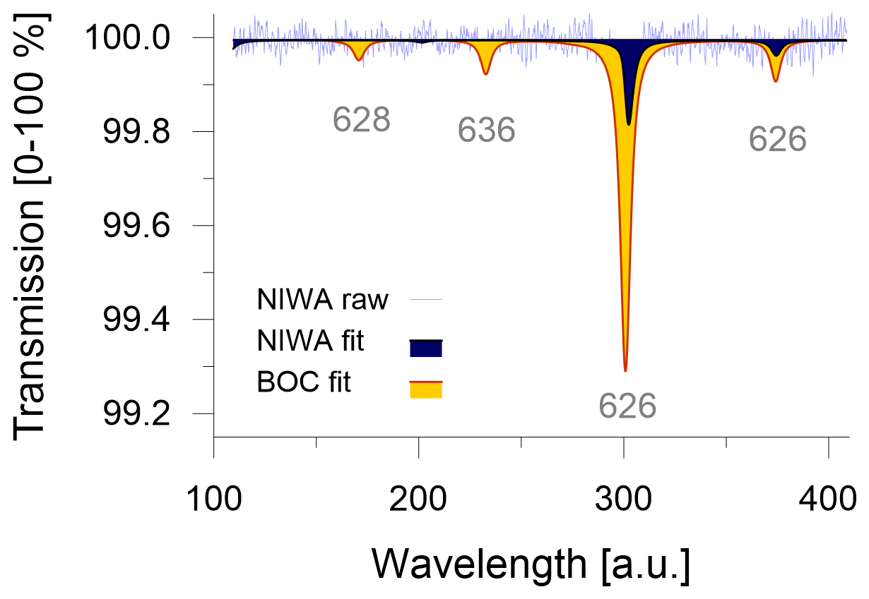
Figure 2Size of CO2 blank in CO2-free air and transmission (%) over artificial units (a.u.), provided by Delta Ray. Raw (light blue) and fitted (dark blue) data from CO2-free air made at NIWA in comparison with fitted spectra of BOC's ultra-zero-grade air (orange).
3.3 CO2-free air from purified natural air
CO2-free air can also be prepared by removing CO2 from natural air, which minimises the potential to alter the composition of the air matrix. For the 2015 campaign, we sourced ultrapure air from Scott-Marrin (now Linde Gas & Equipment Inc., PA, USA), which is made from purified natural air (Scott-Marrin, Lori Thomas, personal communication, via email on 16 August 2014). In the 2018 campaign, we prepared CO2-free air in NIWA's atmospheric laboratory. Therefore, we use an oil-free compressor (Sweet Air, SA-6E, RIX, California, USA) with a 13X molecular sieve trap (8–12 mesh Sigma-Aldrich) on the compressor inlet in combination with a chemical CO2 scrubber (Carbosorb, Elemental Microanalysis, Devon, UK) on the compressor outlet and filled a 30 L cylinder to 50 bar.
The CO2-free air produced at NIWA showed a transmission of 0.2 % (Fig. 2). Based on the experiments with the ultra-zero-grade air from BOC, we estimate the CO2 blank in the CO2-free air produced at NIWA to be ≤ 0.5 ppm as well. Because the added Carbosorb trap in the experiments with the ultra-zero-grade air from BOC produces CO2 blanks that are indistinguishable from the CO2 blank in the CO2-free air made at NIWA, we conclude that adding the Carbosorb trap not only minimises the CO2 blank as much as possible but it also homogenises the CO2 blanks between different CO2-free air cylinders, which would minimise long-term variability.
Measurements of the O2 N2 ratio in the CO2-free air prepared at NIWA confirmed the natural composition of the air matrix was preserved during the purification step. Because of that, we assume that natural Ar N2 ratios were preserved as well and that atmospheric measurements referenced with purified natural air as CO2-free air do not create an accuracy offset due to pressure broadening. In comparison to the ultra-zero-grade air from BOC with an uncertainty of the O2 mole fraction of ±1 %, CO2-free air produced with this technique also guarantees a minimal variability in the air matrix between different CO2-free air cylinders and hence minimal accuracy offsets in long-term measurement series.
3.4 Accuracy offsets due to pressure-broadening effects in CO2-free air
To assess the effect of the different CO2-free carrier gases on the isotope measurements, we measured the two cylinders, QC-4 and QC-5 (Table 1), on the Delta Ray setup, using Ref-1 and different carrier gases: (i) CO2-free air prepared at NIWA, (ii) ultra-zero-grade air from BOC and (iii) ultra-zero-grade air from BOC with a Carbosorb trap to reduce the CO2 blank. We found systematic variation in the measured values. While the measurements with the CO2-free air prepared at NIWA produced accurate isotope values in QC-4 and QC-5 within 0.2 ‰, measurements made with the ultra-zero-grade air from BOC resulted in offsets in the range of +1.14 ± 0.11 ‰ for δ13C-CO2 and of +0.15 ± 0.04 ‰ for δ18O-CO2. Reducing the CO2 blank in the ultra-zero-grade air from BOC resulted in slightly larger offsets of +1.24 ± 0.13 ‰ for δ13C-CO2 and in comparable offsets of +0.17 ± 0.03 ‰ for δ18O-CO2. This suggested that the air matrix effect was dominating the offset. We were unable to further determine whether this effect was due to the complete lack of Argon or the uncertainty in the O2 mole fraction. However, this experiment highlighted that the ultra-zero-grade air from BOC was not a suitable CO2-free air for the Delta Ray system. Therefore, we operated the Delta Ray with purified natural air as carrier gas.
4.1 Allan deviation
We determined the Allan deviation of an earlier version of the Delta Ray analyser during the 2015 campaign using QC-1 and find minimum values of 0.03 ‰ for both δ13C-CO2 and δ18O-CO2 and < 0.01 ppm for CO2 for integration times of 200 to 300 s (Fig. 3). These values are comparable to the findings of Braden-Behrens et al. (2017). We use our Allan deviation results in the design of our measurement sequence and schedule blocks between 200 and 300 s for air and QC gases (Sect. 2.4).
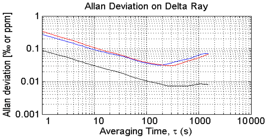
Figure 3Allan deviation determined in QC-1: blue is δ13C, red is δ18O and black is CO2, determined during the 2015 campaign.
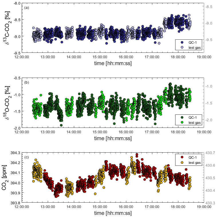
Figure 4Sudden and synchronous shift in both δ13C-CO2 (a) and δ18O-CO2 (b) affecting the measurement of two gases (QC-1 and another test gas cylinder) during laboratory tests. Shifts in isotope traces are not reflected in CO2 mole fractions (c). Causes of the isotope shifts are unknown.
4.2 Instrument stability during 6 h of QC gas measurements
To test the instrument stability of the Delta Ray in the laboratory prior to deployment at BHD, we measured sequences of QC-1 and another test gas cylinder over 6 h. After 5 h, we observed a sudden 0.4 ‰ shift in both δ13C-CO2 and δ18O-CO2 traces that occurred simultaneously for both gases, while the mole fraction measurements of both gases remained unaffected (Fig. 4). We have no explanation for the sudden shifts at this point but can think of two potential causes for this artefact.
- i.
The Delta Ray experiments were performed in a laboratory in which the temperature was not tightly controlled. Because the laboratory had no external walls or windows, temperature fluctuations were likely below 0.2 ∘C min−1, which Thermo specifies as acceptable temperature gradients. While we cannot rule out that a greater temperature change occurred, we think it is unlikely that the temperature in the laboratory suddenly changed dramatically. The experiment was made during the period of core working hours, when both the traffic in and out of the laboratory as well as the magnitude of traffic-induced temperature changes are at their maximum. If the laboratory temperature was not suitable for the Delta Ray, we would expect similar shifts during the first 5 h of this experiment, which we did not observe.
- ii.
We speculate that instabilities during the referencing step may have caused that artefact, which would create a simultaneous shift in both QC gases of identical magnitude. We think that this is the most likely explanation; however, we have no means to support this hypothesis. Interestingly, we notice a significant variability in the CO2 mole fraction measurements in Fig. 7 of Braden-Behrens et al. (2017) during measurements of their target gas, which is not reflected in their isotope traces. Furthermore, Fig. 7 in Braden-Behrens et al. (2017) shows the same pattern of sudden, synchronous changes in the δ13C-CO2 and δ18O-CO2 measurements of the target gas that we observe and describe here. To monitor such artefacts in the following experiments and to be able to correct for such effects, we measured two independent QC gases in every measurement sequence to apply a calibration scheme that is not entirely based on Ref-1. This enables unambiguous identification of whether instability originates from the Delta Ray instrument or the reference gases, and it provides the means to remove affected data or to correct for such effects.
5.1 The BHD site
The Delta Ray was deployed at BHD, located on the edge of an 85 m southward-facing cliff, overlooking the Southern Ocean (41.4083∘ S, 174.8710∘ E; Fig. 5). BHD lies within a regional park at the southern tip of the greater Wellington region with a population of 520 000. Atmospheric dynamics at BHD are highly variable and complex but show a distinct pattern that is described in detail by Brailsford et al. (2012) and Steinkamp et al. (2017). The topography of New Zealand's North Island and South Island deflects the flow path of advected air masses so that the resulting wind direction at BHD ranges between either north-west to north or south-west to south-east most of the time (Fig. 6).
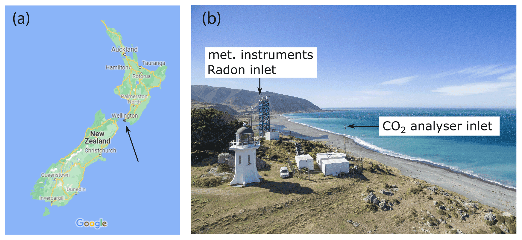
Figure 5(a) Arrow highlights the location of BHD in New Zealand (© Google Maps 2021). (b) Aerial photograph of BHD (provided by Dave Allen, NIWA).
When the air is advected from between north-west to north, the air has most likely passed over New Zealand's North Island and potentially includes a significant terrestrial signal. In some cases, air arrives at BHD from true north but has been deflected from further west to south-west where it has passed over the Tasman Sea and therefore does not carry a clear terrestrial signal at all. Furthermore, it may have passed over the northern parts and the west coast of New Zealand's South Island, in which case it potentially includes a terrestrial signal. Similarly, air advected from south-west to south has potentially passed over the east coast of New Zealand's South Island, a region marked by major cities and agricultural activity. In summary, air masses advected from either north or south may include a terrestrial signal but may also represent oceanic air. Only air advected from between south to south-east has originated from the Southern Ocean and has not been in contact with land masses for many days. These air masses are amongst the cleanest on the planet and are representative of Southern Ocean baseline air. During baseline conditions, the variability of CO2 mole fractions can be less than 0.1 ppm over several hours and even days (Brailsford et al., 2012; Stephens et al., 2013; Steinkamp et al., 2017). In contrast, northerly air masses that contain a terrestrial CO2 signal are likely to include anthropogenic CO2 emissions from urban areas in the greater Wellington region as well. During periods of low wind speeds, the measured CO2 signal can be dominated by local biogeochemical CO2 fluxes, where the short-term variability in CO2 mole fractions can exceed 10 ppm (Stephens et al., 2013; Steinkamp et al., 2017). However, the short-term variability in CO2 isotope ratios has not yet been quantified during such conditions at BHD.
Flask samples are routinely taken during baseline events and include the analysis of CO2 isotope ratios at NIWA's atmospheric laboratory in Wellington (Ferretti et al., 2000), as well as for intercomparison programmes with the Scripps Institute of Oceanography and the Institute of Arctic and Alpine Research (INSTAAR) (Moss et al., 2018). The δ13C-CO2 time series from BHD shows a variability that is typically within 0.2 ‰ per year and a long-term trend of ∼ 0.3 ‰ per decade towards 13C depletion, largely a result from continuously added CO2 from fossil fuel combustion, referred to as the Suess effect (Keeling et al., 2017).
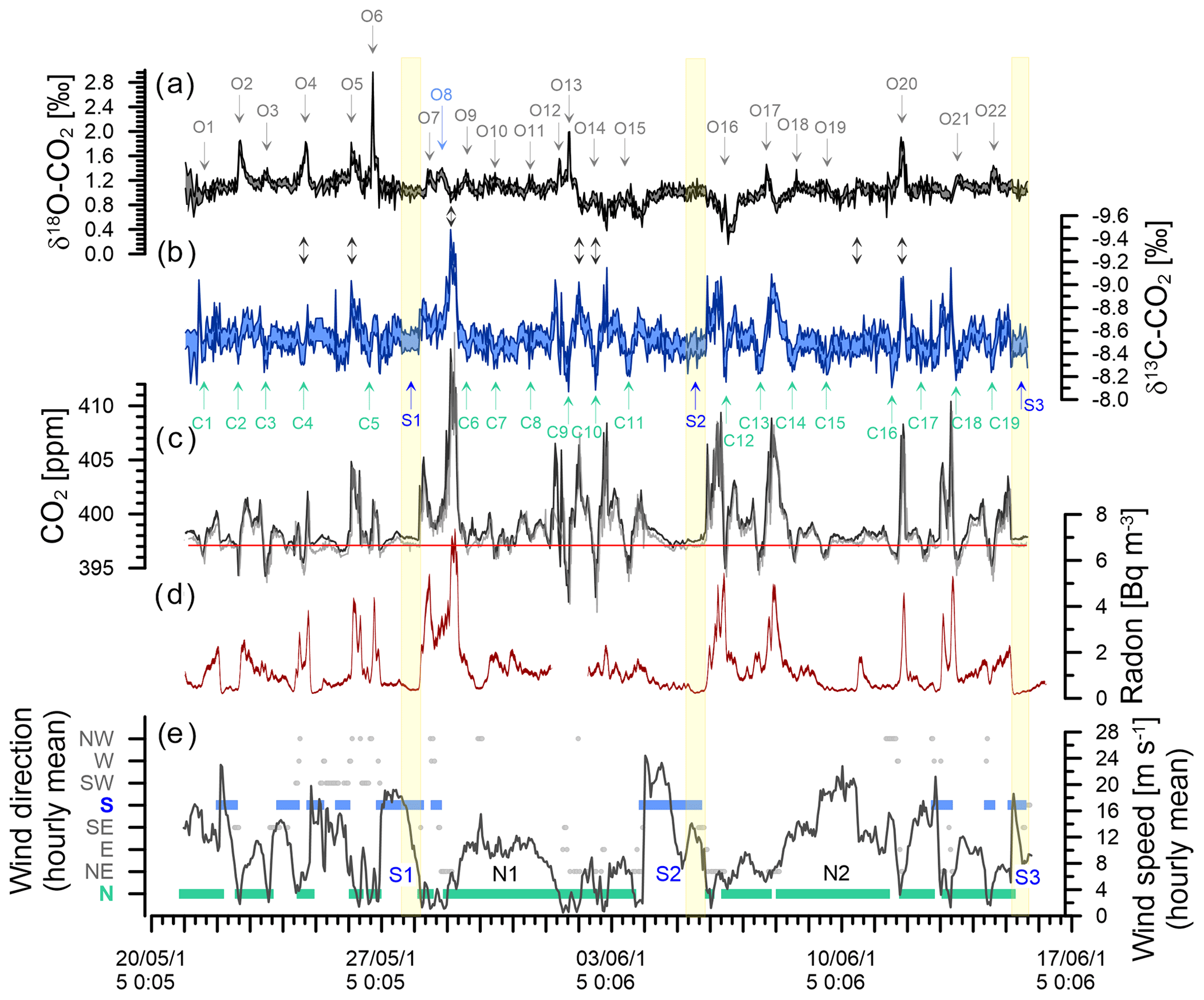
Figure 6Observations during the deployment at BHD (Sperlich et al., 2022). Delta Ray time series of δ18O-CO2 (a) and δ13C-CO2 with inverted y axis (b). CO2 mole fractions measured with Delta Ray (black) and Siemens (grey) with the average of the Siemens analyser for baseline CO2 measured during S2 indicated in red (c). Coloured shading in panels (a), (b) and (c) indicates the standard deviation of the measurement averages of the Delta Ray measurements. Events in the δ18O-CO2 and δ13C-CO2 time series are numbered from O1 to O22 and C1 to C19, respectively. Panel (d) shows the radon time series and panel (e) hourly averages of meteorological data. Southerly and northerly wind events are highlighted in blue and green, respectively. Wind speed is displayed by the black line. The yellow boxes highlight the most stable periods of the three significant southerly events S1, S2 and S3.
The BHD observatory is home to many different analytical systems. Continuous measurements of CO2 mole fractions have been performed at BHD since 1972. A Siemens Ultramat 3 analyser (Siemens AG, Karlsruhe, Germany) was used from 1985–2016 (Brailsford et al., 2012), while a Picarro G2301 analyser was installed in 2011 (Steinkamp et al., 2017), which has since then been upgraded to a Picarro G2401. A radon analyser was built and installed in 2015 by the Australian Nuclear Science and Technology Organisation (ANSTO, Lucas Heights, NSW, Australia), providing half-hourly average data that indicate the degree to which the measured air mass has been in contact with land masses before reaching BHD (Williams et al., 2011; Chambers et al., 2016). Radon measurements were corrected for the detector's response time (Griffiths et al., 2016). The tower at BHD is equipped with a range of meteorological sensors at 12 m above ground level (Fig. 5). Wind data are measured by the 2-D ultrasonic anemometer (Wind Observer II, Gill Instruments, UK), which was installed in May 2013. The raw wind components are measured at 2 Hz and converted to a 3 s average. The 3 s vector components are averaged to 10 min and hourly wind statistics and stored with other meteorological variables in the station data logger (CR1000, Campbell Scientific Inc, USA). Wind characteristics of the site are described by Stephens et al. (2013). The temperature in the laboratory where the Delta Ray was operated was controlled to 19.5 ± 1.5 ∘C, while larger temperature changes may occur during weekly maintenance visits.
5.2 Wind direction, wind speed and radon variability during Delta Ray deployment at BHD
Because the variability of CO2 mole fractions measured at BHD is strongly controlled by atmospheric advection (Brailsford et al., 2012; Stephens et al., 2013; Steinkamp et al., 2017), we expected that this also applies to the isotopes of CO2. Therefore, we will briefly describe characteristics of selected advection patterns that were observed during the Delta Ray deployment at BHD. We support the interpretation of our meteorological observations from BHD with back trajectories from the Hybrid Single-Particle Lagrangian Integrated Trajectory model (HYSPLIT), an atmospheric transport and dispersion model (Stein et al., 2015; Rolph et al., 2017). Figure 6 shows 30 min averages of radon data and hourly averages of both wind speed and wind direction from BHD. Wind direction data are clustered into eight sectors of 45∘, i.e. with the centres of clusters north and south being 360/0 and 180∘, respectively.
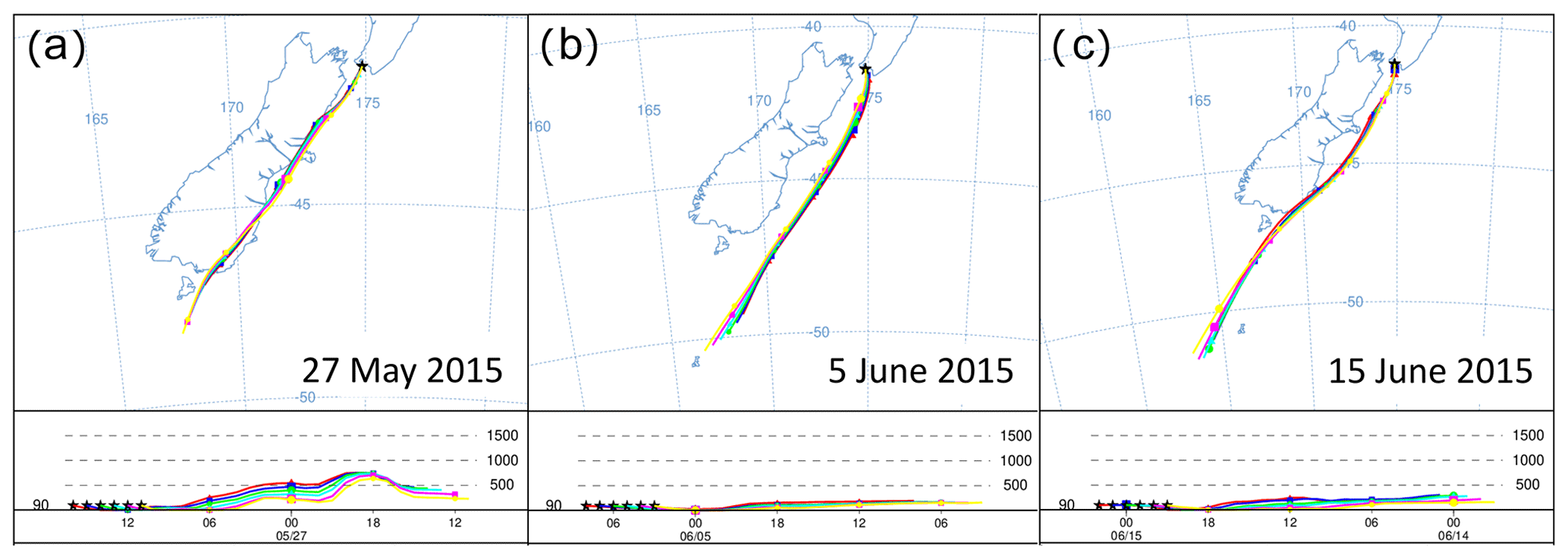
Figure 7HYSPLIT back trajectories (24 h) for the air measured during S1, S2 and S3, with a 1 h interval between displayed trajectories. The selected timing is consistent with the final 6 h of each event displayed in Fig. 16 with the lowest radon counts.
We observed three significant southerly events resulting in baseline/or near-baseline CO2 values on 27 May, 5 June and 15 June of 2015 (S1, S2 and S3 in Fig. 6). These three southerlies are generally marked by some of the lowest radon levels in the record, suggesting the measured air had no significant contact with land masses during the days before advection to BHD. While S2 fulfils the strict requirements for a baseline-air event (Brailsford et al., 2012; Steinkamp et al., 2017) between 08:30 and 18:30 NZST on 5 June 2015, both S1 and S3 are not classified as baseline-air events. The accuracy of this classification is corroborated by HYSPLIT back trajectories for S1 and S3, showing that the air has travelled over New Zealand's South Island before it was measured at BHD, suggesting that air from both S1 and S3 may contain a terrestrial component. Indeed, the radon levels during S1 are slightly higher than those of S2 and S3, thereby supporting the potential for a small terrestrial component during S1, while the radon signal during S2 and S3 is indistinguishable. However, back trajectories show that air masses measured during S2 have been advected from the Southern Ocean, without direct contact to New Zealand's South Island (Fig. 7), in line with our radon observations.
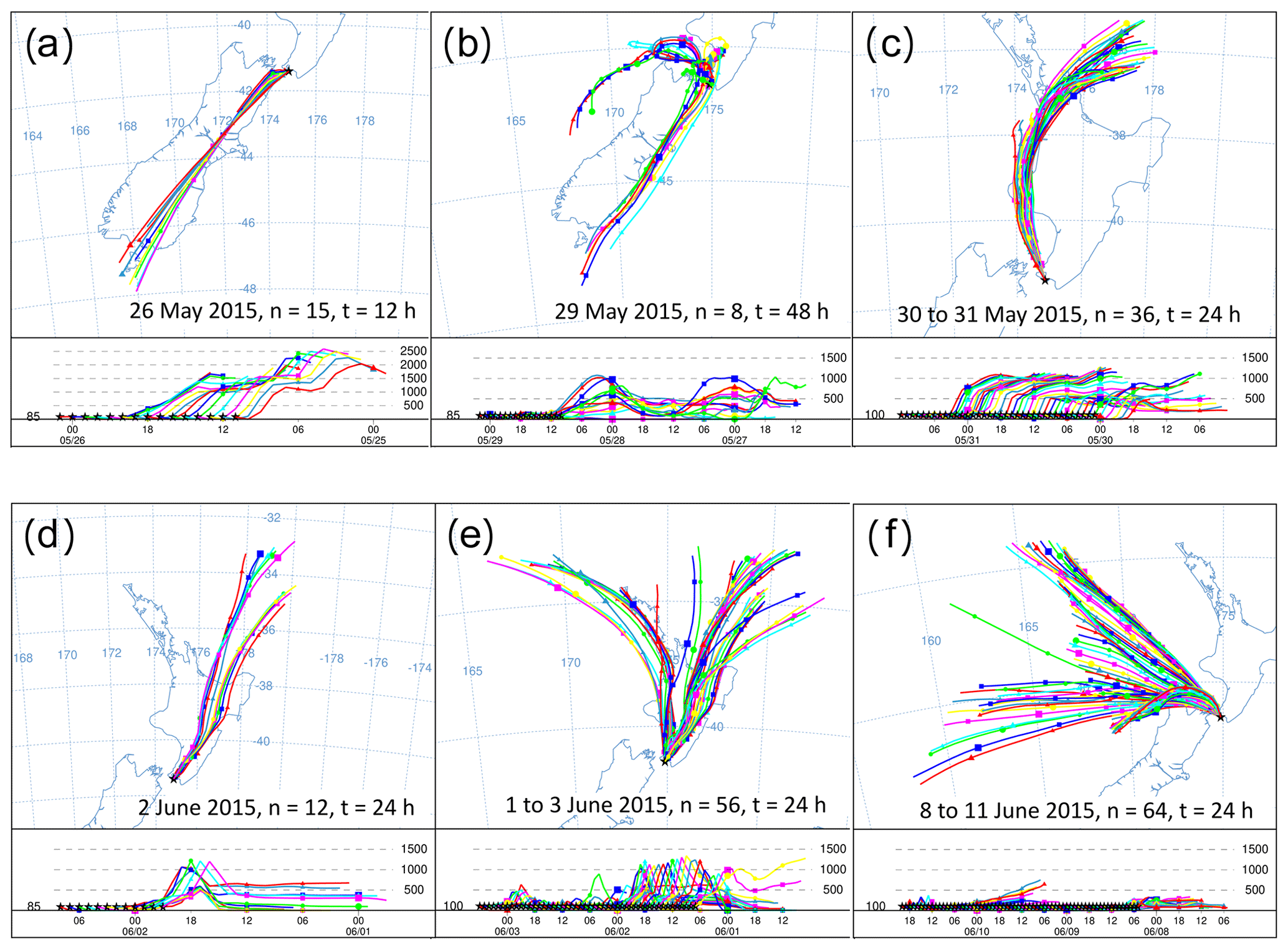
Figure 8HYSPLIT back trajectories from six events in the Delta Ray time series. Each panel shows the history of air that was measured at the stated date. Intervals between trajectories are 1 h, n indicates the number of trajectories in the panel and t represents the trajectory length in hours.
Furthermore, we observe two long-lasting northerly events from 29 May to 1 June 2015 and from 8 to 11 June 2015 (N1 and N2 in Fig. 6). While the average hourly wind speed of N1 with ∼ 10 m s−1 seems typical for our study period, average wind speeds persistently exceeded ∼ 20 m s−1 during N2. The very low radon levels during N2 are comparable with those from S1–S3, indicating the terrestrial impact on the measured CO2 during N2 was small. Back trajectories for the N2 event show that the air was indeed advected from the ocean, with very limited contact to land masses before reaching BHD (Fig. 8f).
We find that the deployment at BHD provides an analytically challenging environment for the Delta Ray analyser, enabling the assessment of its capability to resolve very small to moderate changes in CO2 mole fractions and isotope ratios. Particularly the three southerlies (S1–S3) with very similar properties provide an opportunity to assess the performance of the Delta Ray system under field conditions at a baseline observatory.
6.1 Outlier detection in BHD time series using QC gases
Figure 9 shows all measurements of QC gases during the deployment at BHD as 10 min averages (n = 791). All values in this figure are shown as provided by the Delta Ray, i.e. as measured against Ref-1, without further data processing. On 11 June 2015, the QC-2 was nearing a very low pressure and was replaced with QC-3.
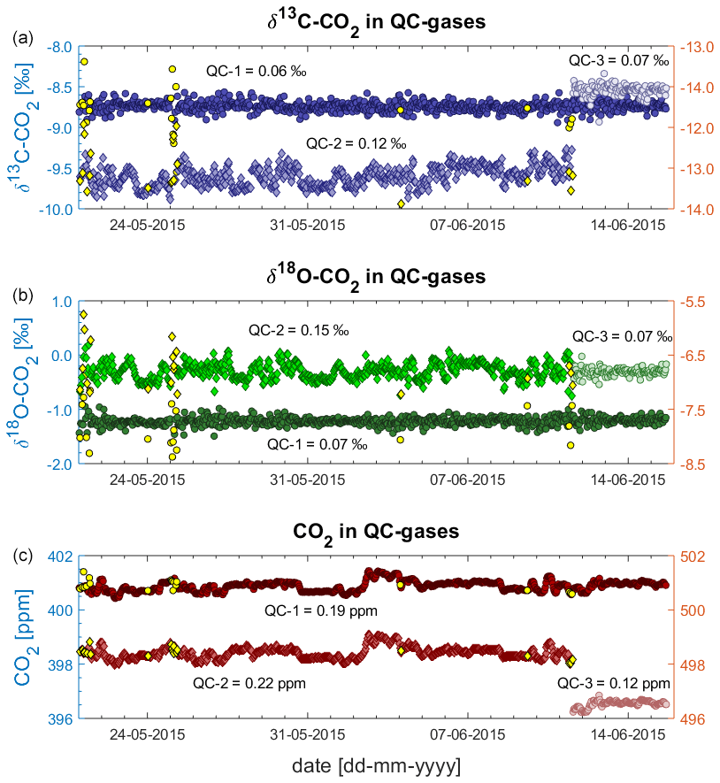
Figure 9QC gas data as measured against Ref-1 during deployment at BHD: δ13C-CO2 (a), δ18O-CO2 (b) and CO2 mole fractions (c). QC-1 and QC-3 on left y axes; QC-2 on right y axes.
The δ13C-CO2 and δ18O-CO2 time series from the QC gases vary around their long-term average and do not show a long-term drift (Fig. 9). However, periods of strong variability that impacts all isotope measurements within the respective 45 min measurement cycle occur on 21 May, on 25 May and from 10 to 11 June of 2015. We did not find a reason for the increased variability. We think that we can rule out that sudden temperature changes have caused the sudden variability, because the most abrupt temperature changes this time of year occur when the door is open during maintenance visits. However, maintenance visits did not coincide with the periods of increased variability in the record.
We find that δ13C-CO2 and δ18O-CO2 are affected in the same order of magnitude and that both isotope traces are affected simultaneously while the CO2 mole fraction data are not affected at all. This pattern is identical to the sudden shift that we observed in earlier laboratory tests (Sect. 4.2) and is similar to observations of Braden-Behrens et al. (2017). Measurement sequences are flagged as outliers (yellow symbols in Fig. 9) when the δ13C-CO2, the δ18O-CO2 or the CO2 measurements of QC-1 deviate from their long-term average by more than 3 standard deviations (3σ). We reject 20 measurement sequences, affecting around 2.5 % of the measurements, resulting in a total of 791 measurement sequences from the 26 d deployment period. For an unknown reason, the measurements of both isotope ratios in QC-2 show a systematic variability, which does not occur in QC-1 and QC-3 (Fig. 9), resulting in generally larger standard deviations of the QC-2 data (Table 3).
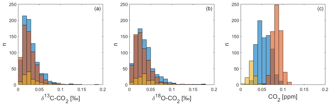
Figure 10Internal reproducibility as the standard deviation (1σ) of the QC gas block averages in each sequence for δ13C-CO2 (a), δ18O-CO2 (b) and CO2 mole fractions (c), with outliers excluded. QC-1 in blue, QC-2 in red and QC-3 in yellow.
6.2 Reproducibility of QC gas measurements during deployment at BHD
Following the removal of outliers, we use the standard deviation (1σ) of the three QC gas measurements within each measurement cycle as an indicator of the reproducibility of the Delta Ray setup. This provides us with 791 values for QC-1, 661 for QC-2 and 130 for QC-3. The histograms in Fig. 10 display the distribution of the standard deviation values, showing that the majority of the δ13C-CO2 and δ18O-CO2 values lie within a range that is comparable to the Allan deviation of 0.03 ‰ (Sect. 4.1 and Fig. 3). This suggests that the Delta Ray system at BHD is operating close to its maximum performance level for isotope ratio measurements during most of the time. In contrast, the histogram for CO2 shows that all standard deviation values from all three QC gases are out of range compared to the Allan deviation of 0.01 ppm (Sect. 4.1). Furthermore, the standard deviations of the CO2 measurements appear in QC gas-specific clusters. The reason for this pattern and the weak performance in CO2 measurements remains unclear; however, we speculate that this is associated with effects in the cylinders or pressure regulators rather than the Delta Ray itself.
6.3 Control of linearity and isotope scale compression during deployment at BHD
We compare the average measurement results for the QC gases obtained by the Delta Ray measurements to the target values determined by GC and GC-IRMS analysis in Table 3. QC-1 and QC-2 were designed to cover a large range in CO2 mole fractions (∼ 97.3 ppm) as well as in δ13C-CO2 (∼ 4.9 ‰) and δ18O-CO2 (∼ 5.5 ‰) to assess the capability of the Delta Ray to make accurate measurements over a large range. Table 3 shows good agreement between the Delta Ray measurements and the target values. This suggests that a potential linearity effect is sufficiently controlled via the linearity calibration of the Delta Ray and that the calibration scheme of the Delta Ray based on Ref-1 and Ref-2 is able to prevent significant scale compression artefacts.
However, the QC-1 corrected data seem to overestimate the CO2 mole fraction in QC-2 by about 0.27 ppm, given a CO2 difference between QC-1 and QC-2 of 97.3 ppm. In comparison, this difference accounts for only 0.01 ppm for QC-3, which had CO2 mole fractions that were very similar to that of QC-1. While this difference is within the combined measurement uncertainty for CO2 mole fractions in both cases, it might be due to inaccurate control of large CO2 variations. If this overestimation in QC-2 was based on a linear process, it would add an error of +0.0028 ppm ppm−1 to the mole fraction measurements. Using this value, we estimate that the CO2 mole fractions in the air measurements of the deployment at BHD would need to exceed or fall below the target value of QC-1 (400.43 ± 0.09 ppm) by > 18 ppm to produce an offset that exceeds the compatibility goal formulated by the WMO, which did not occur during the deployment at BHD. Note that the Delta Ray has the capability for a two-point mole fraction calibration, which we have not utilised during this assessment. It is thus likely that the control of this effect can be improved by a second concentration standard (Thermo, 2014).
6.4 CO2 mole fraction measurements in QC gases
The CO2 mole fraction data from the QC gas cylinders show synchronous variations of similar magnitude (Fig. 9). Interestingly, this feature is similar to observations made by Braden-Behrens et al. (2017), who also found a similar variability in CO2 mole fraction measurements in cylinder air. A linear regression analysis between QC-1 and QC-2 suggests that about 84 % of the variability in the mole fraction measurements in both cylinders can be explained by the same process. This finding gives strong support for using QC-1 as the working standard in the post-processing protocol for CO2 mole fractions. Moreover, this highlights the importance of determining and applying correction factors for every single measurement sequence. It is important to note that the prominent features in the CO2 mole fraction measurements are not reflected in the isotope traces. This suggests that the internal linearity calibration of the Delta Ray is robust for CO2 variations of that magnitude (Fig. 9).
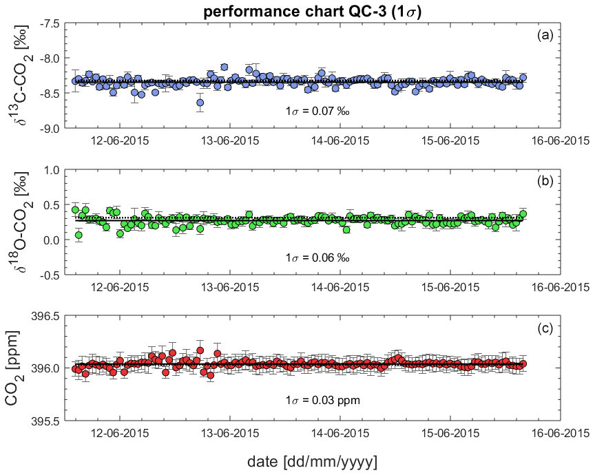
Figure 11Sequence averages for processed δ13C-CO2 (a), δ18O-CO2 (b) and CO2 (c) in QC-3. The standard deviation (1σ) is a measure of the achievable analytical precision.
6.5 Assessment of the instrument performance using QC gas measurements from BHD in the performance chart method
Given the lack of a second QC gas that was measured over the entire campaign and the low quality of the measurements of QC-2, we use the QC-3 time series to assess the reproducibility of the Delta Ray measurements using the performance chart method (Werner and Brand, 2001) in Fig. 11. The performance chart is based on δ13C-CO2, δ18O-CO2 and CO2 values of QC-3, after full corrections have been applied. Error bars represent the fully propagated uncertainty of the measured averages in each sequence. Next, we determine the standard deviation (1σ) of all δ13C-CO2, δ18O-CO2 and CO2 values from all QC-3 measurements as an indicator of the instrument performance (Werner and Brand, 2001). We find a reproducibility (1σ) for δ13C-CO2, δ18O-CO2 and CO2 of 0.07 ‰, 0.06 ‰ and 0.03 ppm, respectively, n = 130, which we use as a measure of achievable measurement precision. Because the variability in isotope ratios of the relatively short time series for QC-3 is similar to the time series of QC-1 spanning 26 d (Figs. 9 and 10), we think this is a representative estimate.
While the precision estimates for both isotope ratios did not meet the WMO network compatibility goal of 0.01 ‰ for δ13C-CO2 and 0.05 ‰ for δ18O-CO2, they did meet the expanded compatibility goal of 0.1 ‰ for both parameters. However, our instrument precision for CO2 mole fractions of 0.03 ppm met the WMO network compatibility goal of 0.05 ppm (WMO-GAW, 2019).
The following sections compare the Delta Ray time series to observations made with well-established measurement systems at BHD. Furthermore, we describe and interpret features in the Delta Ray time series in the context of atmospheric advection, with the objective to highlight the capability of the Delta Ray instrument to resolve the variability of CO2 and its isotope ratios at BHD under field conditions.
7.1 Comparing CO2 mole fraction measurements from Delta Ray and Siemens Ultramat 3 at BHD
We used 5 min average CO2 mole fraction measurements from the Siemens Ultramat 3 gas analyser at BHD (Brailsford et al., 2012; Stephens et al., 2013). To compare Siemens and Delta Ray data, we removed periods when the Siemens was in calibration mode from both time series. Next, we sub-sampled the remaining 5 min averages from the Siemens at the time averages of the remaining Delta Ray data by linear interpolation and used the resulting 738 data pairs for comparison.
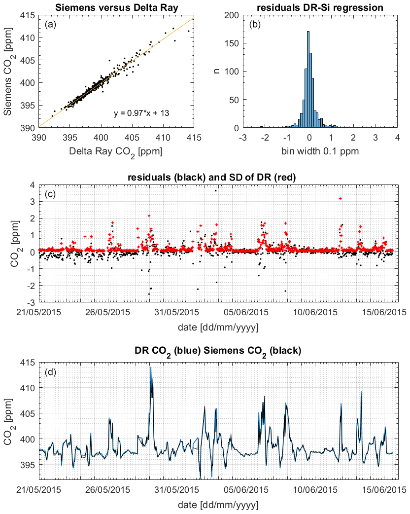
Figure 12(a) Slope and scatter of the regression Siemens (Si) versus Delta Ray (DR). (b) Histogram of residuals. (c) Residuals (black) and 1 standard deviation (1σ) of the DR measurements (red). (d) CO2 mole fractions from DR (blue) and Siemens (black).
Figure 12 displays the CO2 mole fraction data comparison between the Delta Ray and the Siemens analysers. The histogram showed the residuals with a Gaussian distribution, suggesting that the offset was not systematically biased towards either lower or higher mole fractions. The potential scale effect in our Delta Ray setup of 0.0028 ppm ppm−1 produced a maximum bias of 0.04 ppm on the 29 May 2015 (Sect. 6.3). Interestingly, the slope of 0.97 in the comparison confirmed a bias in the Delta Ray data towards higher values (Fig. 12). Out of the 738 data pairs used for the comparisons, 155 or 21 % agreed within the WMO compatibility goal of 0.05 ppm for the Southern Hemisphere, while 287 or 39 % of the data pairs agreed within the WMO compatibility goal of 0.1 ppm for the Northern Hemisphere, respectively (WMO-GAW, 2019). Furthermore, 542 or 73 % of the data pairs agreed within the standard deviation of the mole fraction averages, which amounted up to a few parts per million during times of high CO2 variability in the measured air (Fig. 12). In these cases, the large standard deviation coincided with large residual values, suggesting that the agreement between both time series could be improved through synchronisation of the averaging intervals.
This finding is corroborated by the excellent reproducibility of CO2 mole fraction measurements of QC-3 in the performance chart of 0.03 ppm (Sect. 6.5), suggesting the Delta Ray setup is capable of highly reproducible mole fraction measurements that meet the WMO network compatibility goal.
7.2 CO2 mole fraction observations of the Delta Ray during deployment at BHD
The CO2 mole fractions during the Delta Ray deployment at BHD varied between 392 and 414 ppm, spanning a total range of 22 ppm. The average CO2 mole fraction of 397.09 ppm from the baseline event S2 that occurred on 5 June 2015 is shown with a red line in Fig. 6c.
The most prominent pattern of the CO2 mole fraction time series is the daily cycle, which is typically characterised by CO2 minima between midday and later afternoon when photosynthetic CO2 uptake dominates CO2 fluxes, as well as CO2 maxima at night-time during boundary layer build-up of CO2 from respiration and anthropogenic sources. CO2 peaks are typically accompanied by radon peaks of proportional magnitude (Fig. 6d), highlighting the interplay of CO2 dilution by wind speed versus CO2 accumulation in the boundary layer, as control of the CO2 peak amplitude (Williams et al., 2011; Chambers et al., 2016).
The largest single event of the CO2 time series is the CO2 build-up to 414 ppm in the night-time boundary layer in the early hours of 29 May 2015, also coinciding with the largest peak in the radon time series (Fig. 6c and d). Back trajectories show the air flow leading up to this event (Fig. 8b). In the 48 h before measurement at BHD, the measured air had passed over the cities of Dunedin, Christchurch, Lower Hutt and Wellington in a southerly, before the wind direction changed to northerly and the same air passed over Wellington and Lower Hutt again before measurement at BHD. The amplitude of the CO2 peak was enhanced by the relatively low wind speeds of < 5 m s−1, preventing effective vertical mixing. The advection pattern suggests that both urban CO2 emissions and ecosystem respiration contributed to the elevated CO2 levels.
We observe seven daily CO2 cycles with an amplitude between 10–15 ppm occurring after 1 June 2015. These events are typically associated with air advection across New Zealand's North Island (Fig. 8e) and moderate wind speeds. However, only four of these events coincide with high radon peaks (Fig. 6d). The data gap in the radon time series on 1 June 2015 is because the instrument is in calibration mode on the first day of every month. Furthermore, nine daily CO2 cycles with amplitudes between 5–10 ppm and three with amplitudes between 1–5 ppm occur in the record, where most of them have a corresponding signal in the radon time series. However, some exceptions occur where days with ∼ 6 ppm (14 June 2015) or even ∼ 13 ppm (2 and 3 June 2015) amplitudes of the daily CO2 cycle do not show a significant counterpart in the radon time series.
Both the amplitude and the timing of these 20 daily CO2 cycles are controlled by wind direction and wind speed. In general, the amplitude of the daily CO2 mole fraction cycle appears in an inverse relationship with wind speed in the measurements of terrestrial air, where higher wind speeds coincide with smaller amplitudes and peak widths in the daily CO2 cycle. For example, the largest CO2 peak during 29 May 2015 occurred when wind speeds were below 5 m s−1. In contrast, the daily CO2 cycle was strongly dampened to values between 2 and 4 ppm at persistent wind speeds of ∼ 10 m s−1 between 30 and 31 May 2015 (N1), when the air was advected along the west coast of the North Island (Fig. 8c). We observed CO2 cycles with an even smaller amplitude of ∼ 1 ppm between 9 and 10 June 2015 (N2). Interestingly, CO2 minima and maxima appear out of phase with the expected timing of daily CO2 cycle during these days. While the recorded wind direction is true north, back trajectories show that the air has been deflected and in fact originated from the Tasman Sea, suggesting that the small CO2 variability could be a distant signal (Fig. 8f).
As expected for air with oceanic properties, we observe no daily CO2 cycle during S1–S3. With the onset of a southerly event, an ongoing daily cycle diminishes, and CO2 mole fractions begin to approach baseline values (Fig. 6c). Because the air during a southerly event becomes more stable and cleaner with duration of the event, we focus on the final 6 h period within each S1, S2 and S3. We found similar CO2 mole fractions for S1 and S3 of 397.29 ± 0.07 and 397.21 ± 0.05 ppm, respectively, while the baseline-air event S2 is marked by slightly lower CO2 mole fractions of 397.09 ± 0.11 ppm. HYSPLIT back trajectories show the S2 has not been in contact with land masses prior to the measurements, while air masses measured during both S1 and S3 have been in contact with New Zealand's South Island (Fig. 7). The small difference between S2 on the one hand and both S1 and S3 may thus be a result from an additional component of terrestrial CO2 during S1 and S3.
7.3 δ13C-CO2 observations of the Delta Ray during deployment at BHD
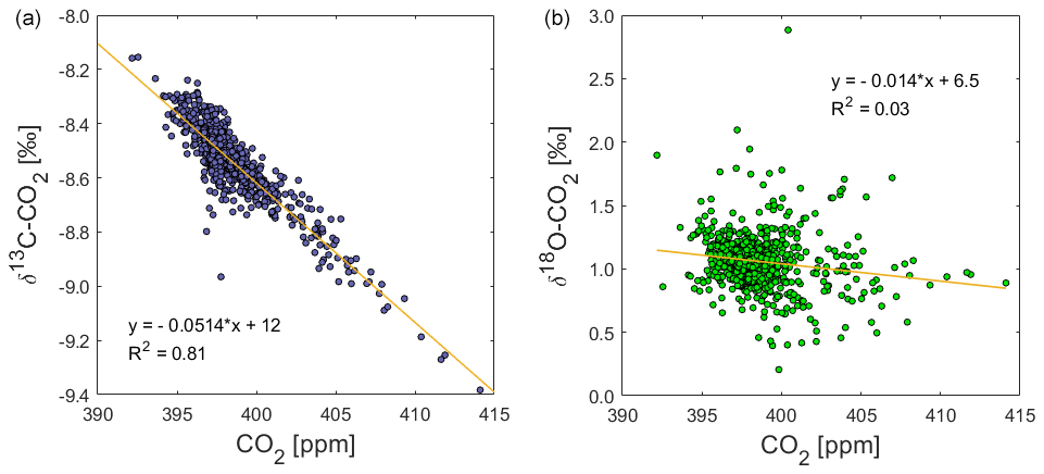
The δ13C-CO2 data from the field deployment at BHD appear with an average value of about −8.54 ± 0.14 ‰ (average ±1σ). The most prominent features in the δ13C-CO2 time series are the systematic daily cycles that occur in concert with CO2 mole fractions (Fig. 6b). The δ13C-CO2 maxima in observed daily cycles are marked with C and are numbered in the δ13C-CO2 time series (Fig. 6b). As expected, the amplitude of the daily cycle in δ13C-CO2 is negatively correlated with that of CO2 mole fractions, where daily δ13C-CO2 maxima correspond to daytime minima in CO2 mole fractions. The R2 suggests that 81 % of the variability in δ13C-CO2 could be explained by the variation of CO2 (Fig. 13).
This pattern is generally consistent with CO2 uptake by plants, which preferentially assimilate 13C-depleted CO2, leading to 13C-enriched CO2 in the remaining atmosphere (Ciais et al., 1995a; Bowling et al., 2005; Braden-Behrens et al., 2017). In line with Bowling et al. (2005) and Braden-Behrens et al. (2017), we observe a strong δ13C-CO2 depletion during the build-up of CO2 in the night-time boundary layer, which coincides with radon build-up, highlighting that terrestrial CO2 fluxes caused this variability at our coastal observation site. This pattern is expected as the ground-level CO2 increase is caused by ecosystem respiration (around −27.5 ‰ in C3-plant-dominated ecosystems) or anthropogenic sources (−26 ‰ to −44 ‰), both of which are strongly depleted in 13C compared to atmospheric δ13C-CO2 (Vardag et al., 2016; Braden-Behrens et al., 2017).
We observe 19 δ13C-CO2 events (C1–C19). Daily cycles in δ13C-CO2 that are statistically significant but close to the limit of detection are observed at amplitudes of the daily cycle in CO2 mole fractions as low as 2 to 3 ppm (e.g. C6, C7, C15, C17). This is confirmed by the following back-of-the-envelope calculation. Using the linear regression of the correlation between CO2 mole fractions and δ13C-CO2 (Fig. 13), we can calculate a minimum difference in CO2 mole fractions that would theoretically result in a significant δ13C-CO2 difference of at least twice the δ13C-CO2 measurement uncertainty of ±0.07 ‰ (Fig. 11).
We find that the Delta Ray setup as described and operated at BHD requires a CO2 variability of at least ∼ 2.6 ppm in order to measure a δ13C-CO2 signal that exceeds 0.14 ‰ or twice the analytical uncertainty. Note that this estimation is critically dependent on the isotopic composition of the locally prevailing CO2 source and is therefore specific to the deployment site.
The majority of observed daily CO2 cycles exceeds an amplitude of 2.6 ppm (Sect. 7.2), resulting in a typical amplitude of daily δ13C-CO2 cycles between 0.2 and 0.7 ‰, thereby exceeding the measurement uncertainty by a factor of 3–10, respectively. Our observations show that the Delta Ray setup is able to resolve most δ13C-CO2 variations at BHD that are associated with terrestrial CO2 fluxes. This assessment has so far provided critical indicators of instrument performance such as the achievable instrument precision and the limit of the analytical resolution under field deployment conditions.
7.4 Instrument performance as the limiting factor of the signal size requirement for application of Keeling plot analysis
In this section, we assess the limitations of the analysis that can be done on the data from the field-deployed instrument using Keeling plot analysis (KPA). Following the recommendations of Zobitz et al. (2006) for data with small CO2 ranges, we use the Model 1 regression (ordinary least squares) and the standard error as uncertainty of the determined intercept in our KPAs. Bowling et al. (2005) point out that this prevents an erroneous bias of strongly 13C depleted intercept values at the lowest CO2 ranges, which seems to produce realistic intercept results from our data (e.g. Fig. 14b). We selected 12 events in the CO2 and δ13C-CO2 time series (Fig. 6b and c) ranging from the smallest (2 ppm) to the largest (16 ppm) CO2 mole fraction variations. Selected events include six CO2 peaks and six CO2 troughs, resulting from both night-time boundary layer CO2 build-up and photosynthetic CO2 uptake, respectively.
The CO2 amplitude of these events is well correlated with the amplitude in δ13C-CO2 (Fig. 14a) with a coefficient of correlation of 0.97. As expected from the findings of Pataki et al. (2003), Bowling et al. (2005) and Zobitz et al. (2006), the uncertainty of our intercepts increases when the range of CO2 and δ13C-CO2 is small (Fig. 14c and d). However, it is noteworthy that the data of Pataki et al. (2003) require a minimum CO2 range of 75 ppm to achieve intercept uncertainties of ≤ 1 ‰, whereas Bowling et al. (2005) apply a lower threshold of ≤ 40 ppm. In comparison, we find intercept uncertainties of ±5 ‰ at CO2 ranges of ∼ 2.5 ppm and of ∼ 1 ‰ at CO2 ranges ≥ 10 ppm (Fig. 14c), which Zobitz et al. (2006) reported as an acceptable uncertainty level. For further comparison, Pieber et al. (2021) filter their multi-year data to exclude CO2 variations < 3 ppm and cluster their data for intercept uncertainties of 1 ‰, 2 ‰, 3 ‰ and 4 ‰, which indicates the performance of their instrument is superior to that of the Delta Ray system presented here. Zobitz et al. (2006) model the improvement in the uncertainty of the intercepts with improvement of the measurement precision for isotope ratios. Given the superior measurement precision of the Delta Ray setup of ±0.07 ‰ (Sect. 7.2) in comparison to the setup described by Bowling et al. (2005), the uncertainty of the intercepts in our KPAs is smaller as expected. While this proves the gain in the interpretability of measured data with the instrument performance of the Delta Ray, the comparison with Zobitz et al. (2006) and Pieber et al. (2021) shows that further improvement of instrument precision would be desirable to further improve the usefulness of observations.
7.5 Keeling plot analysis using δ13C-CO2 observations from BHD
The intercepts of all KPAs in Fig. 14b range between −23 ‰ and −33 ‰ with an average of −30 ‰, which is around −3 ‰ more depleted in 13C than the typical intercept values both Pataki et al. (2003) and Bowling et al. (2005) report. However, our intercept values are in the range that Vardag et al. (2016) report from an urban site and Braden-Behrens et al. (2017) find at a forest site, as well as in the range that Pieber et al. (2021) report from observations at a background air location.
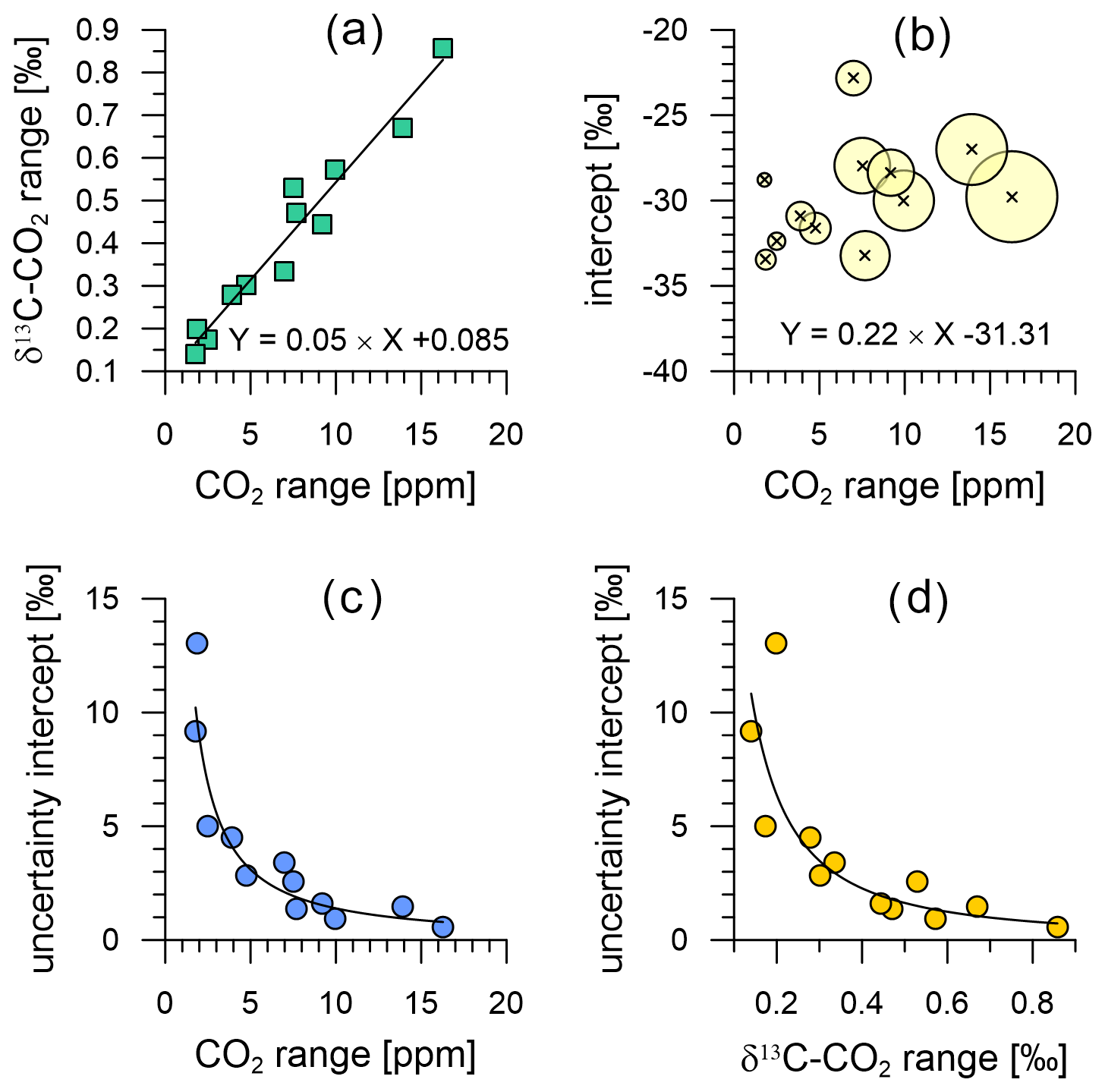
Figure 14Relationship between the variations in CO2 and δ13C-CO2 of the 12 events used for KPA (a), as well as their intercept as a function of the covered CO2 range (b). The bubble size in (b) scales with the range in δ13C-CO2 covered within the KPA event. Uncertainty of the intercept (standard error) as a function of the range in CO2 (c) and δ13C-CO2 (d).
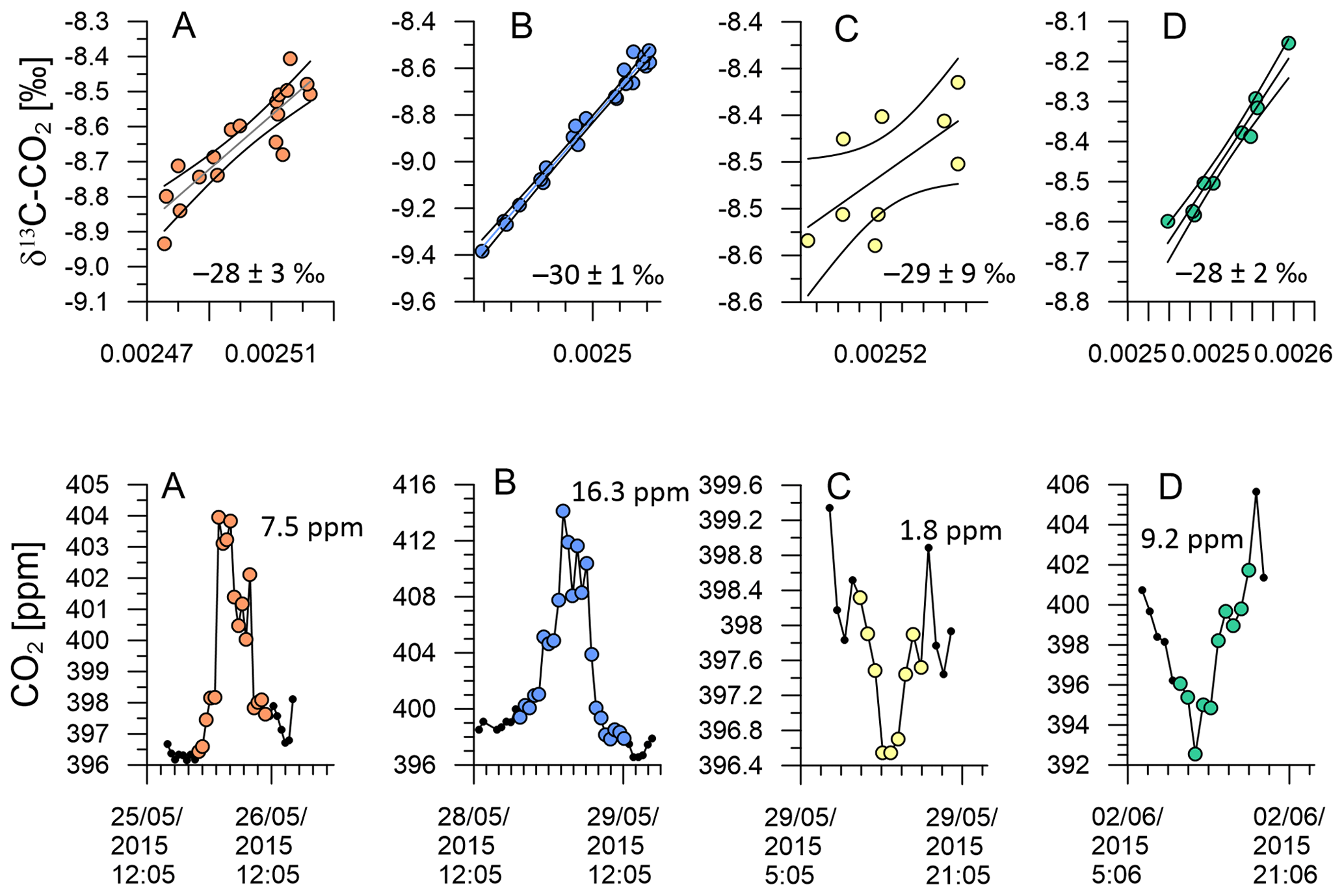
Figure 15KPA with 95 % confidence interval and standard error for the intercept of A–D (top). CO2 variation of events A–D (bottom).
Figure 15a and d show KPA intercepts that are in good agreement with the values from Pataki et al. (2003) and Bowling et al. (2005), i.e. the CO2 build-up in the night-time boundary layer on 26 May 2015 and the photosynthetic CO2 drawdown on 2 June 2015 with intercept values of −28 ± 3 ‰ and −28 ± 2 ‰, respectively. The intercepts from both events are in the expected range for C3-plant-dominated ecosystems. Indeed, Fig. 8a and d show that the air was advected over the central South Island on 26 May 2015, while it passed over the central North Island on 2 June 2015. The central parts of both islands are predominantly either forest or farmland, while urban areas are mostly in the coastal regions, which corroborates the KPA result.
These two events are marked by a CO2 range of 7.5 and 9.2 ppm, respectively (Fig. 8a and d). In contrast, the photosynthetic uptake event on 29 May 2015 is marked by an intercept of −29 ‰ with a large uncertainty of ±9 ‰ due to the small CO2 range of 1.8 ppm (Fig. 8c). This event directly followed the largest CO2 peak in our time series. Back trajectories for the daytime of 29 May 2015 (not shown) indicate that over the previous 48 h, the measured air was advected from the Tasman Sea and has only been in contact with land masses in the last hour before measurement. Despite the large uncertainty of the intercept, its value of −29 ± 9 ‰ rules out that marine processes have caused the small CO2 decrease, because oceanic CO2 uptake does not discriminate strongly against 13C.
In contrast, the night-time build-up of CO2 in the early hours of the 29 May 2015 is the largest feature of our time series. For that event, our KPA shows an intercept of −30 ± 1 ‰ (Fig. 15b), which is slightly more depleted in 13C than what we would expect for respiration of C3 plant ecosystems (Pataki et al., 2003; Bowling et al., 2005). Back trajectories from that event show that the air measured during this event has passed over the urban areas of Wellington and Lower Hutt (Fig. 8b), which likely resulted in the impact of additional urban CO2 emissions in our measurements. Urban CO2 can explain the 13C depletion of the intercept, because, besides wood, isotopically depleted natural gas is widely used as fuel for residential heating in the Wellington region.
It is important to keep in mind that the nature of observations by Pataki et al. (2003), Bowling et al. (2005), Zobitz et al. (2006) and Braden-Behrens et al. (2017) is fundamentally different from our study as well as from that of Vardag et al. (2016) and Pieber et al. (2021). Due to the remote location of our study site and that of Pieber et al. (2021), observed CO2 and δ13C-CO2 variations result from a spatio-temporal integration of multiple CO2 processes and different ecosystem types along the air flow path. In comparison, the observations of Pataki et al. (2003), Bowling et al. (2005) and Braden-Behrens et al. (2017) were made within one ecosystem, while those of Vardag et al. (2016) were made in an urban environment. Resulting differences between the intercepts derived in these studies are therefore expected.
7.6 δ18O-CO2 observations of the Delta Ray during deployment at BHD
Over the course of our study period, the δ18O-CO2 measurements vary around a baseline value of +1.1 ‰ (Fig. 6). This value is in the expected range for a coastal site in the mid-latitudes of the Southern Hemisphere, and it is in good agreement with observations from the Commonwealth Scientific and Industrial Research Organisation (CSIRO) at the Cape Grim Observatory (CGO) (Francey and Tans, 1987; Welp et al., 2011). In comparison to δ13C-CO2, the δ18O-CO2 time series does not show a strong correlation with CO2 mole fractions (Fig. 13). The δ18O-CO2 time series shows 22 distinct events with amplitudes that range between 0.1 ‰ and 1.5 ‰, labelled O1–O22 in Fig. 6. All events except O8 occur during northerly wind conditions and are most pronounced during low wind speed. All events except O5 and O20 occur during daytime, while δ18O-CO2 typically declines as radon levels increase with the build-up of the night-time boundary layer (e.g. O2, O4, O6), when the observed daily δ18O-CO2 cycle is a signal of the terrestrial biosphere. Atmospheric CO2 undergoes oxygen isotope exchange with 18O-enriched leaf water (Francey and Tans, 1987; Farquhar et al., 1993; Welp et al., 2011; Cernusak et al., 2016), which is modulated by stomatal conductance that is generally high at daytime and low at night-time (Caird et al., 2007). Most peaks in the δ18O-CO2 record are therefore a result of photosynthetic activity of the terrestrial biosphere. This explains the lack of a δ18O-CO2 signal during S1, S2 and S3, when the air was advected over the ocean (Fig. 7) and had limited (S1, S3) or no (S2) contact with the terrestrial biosphere in the recent past.
Changes in the δ18O-CO2 record suggest that the measured CO2 has been in isotopic exchange with different water bodies of different isotopic compositions. Baisden et al. (2016) show the spatial variability of the isotopic composition of precipitation in New Zealand. In general, δ18O in precipitation becomes more depleted with (i) increasing distance to the Equator (latitudinal gradient), (ii) increasing distance to the precipitation source (ocean water) and (iii) increasing altitude (Dansgaard, 1964; Baisden et al., 2016). In a very simplified approach, we can assume that the spatial isotope pattern of the precipitation creates a corresponding pattern in the isotopic composition of leaf and soil water bodies, which will impact on δ18O-CO2 during isotope exchange accordingly (Farquhar et al., 1993; Cernusak et al., 2016).
An example of this can be observed during 2 to 3 June and 6 June 2015, when δ18O-CO2 appears 0.3 ‰ to 0.6 ‰ more depleted than average, indicating that this CO2 has been in isotopic exchange with 18O-depleted leaf and soil water. In fact, HYSPLIT back trajectories show that air masses measured during this period were predominantly advected from inland regions and higher altitudes (Fig. 8d), where the δ18O of the precipitation is more depleted than in other regions (Baisden et al., 2016).
Interestingly, the night-time events O5 and O20 show an 18O enrichment of 0.7 ‰ to 1.0 ‰, which is accompanied by a simultaneous 13C depletion of ∼ 0.6 ‰ and increased CO2 mole fractions of 7 to 10 ppm. This combined pattern furthermore coincides with peaks in radon (Fig. 6). Back trajectories from O20 (not shown) reveal that the measured air has been advected from the west coast of the South Island, from where it passed over alpine areas as well as over the city of Wellington before it was measured at BHD. It is thus likely that the additional CO2 originated from a combination of anthropogenic sources and ecosystem respiration and had potentially been subject to exchange of oxygen with a water body that was enriched in δ18O-H2O.
Our observations show that the Delta Ray is capable of resolving small changes in δ18O-CO2 and that these measurements enable further analysis of anthropogenic and ecosystem processes along the pathways of advected air masses.
8.1 Variability of CO2 mole fractions during southerlies
Figure 16 zooms into the measurement data from the three southerly periods S1, S2 and S3. Delta Ray and Siemens data show good agreement throughout the events and differences of the event averages (calculated as Delta Ray – Siemens) of −0.03, −0.08 and +0.04 ppm CO2, for S1, S2 and S3, respectively, which is within the compatibility goal of the WMO for S1 and S3 but not for S2. The Delta Ray CO2 data for S2 include one strongly elevated CO2 value towards the end of the event. If this data pair was removed, the disagreement between Delta Ray and Siemens during S2 would increase to −0.11 ppm. Both analysers show S2 with the lowest CO2 mole fractions, which seems plausible given the potential for added terrestrial CO2 during both S1 and S3 (Fig. 7). A possible explanation for the variability between measurements is the different measurement schedules both analysers operate on. While the Delta Ray observations follow a measurement schedule containing only 22 % air measurements per cycle (Table 2), the measurement schedule of the Siemens during southerlies measures air during 50 % of the time and thus makes more than twice as many observations but not necessarily at the same time as the Delta Ray. The difference in timing may explains some differences between the measurements of both systems. However, we would expect the differences to be minimal during southerly events and especially during steady intervals, as is the case for S2.
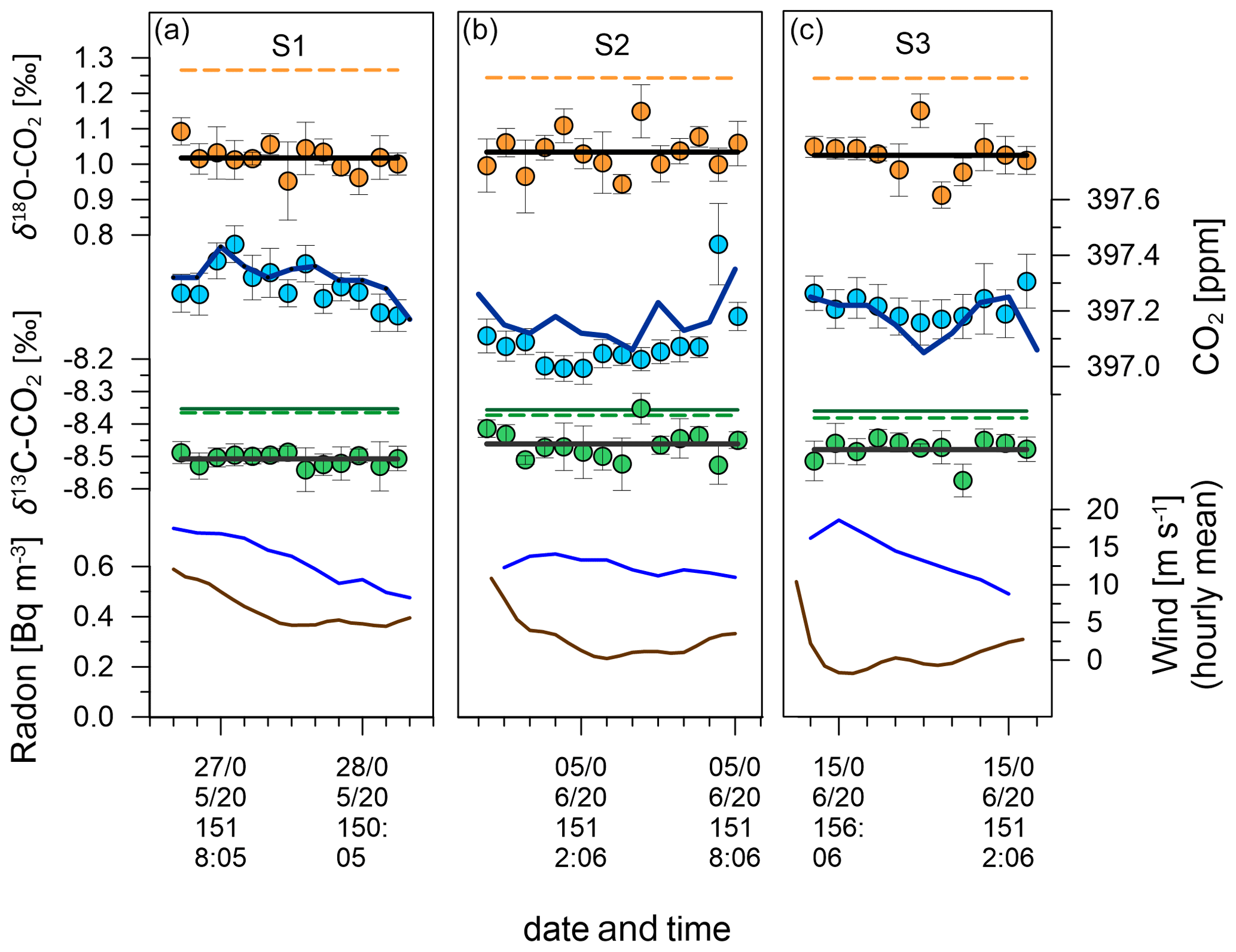
Figure 16Data from southerly events S1 (a), S2 (b) and S3 (c). Radon is shown in brown lines and mean hourly wind speed in blue lines. Green, blue and orange filled circles show average Delta Ray values for δ13C-CO2, CO2 mole fractions and δ18O-CO2, respectively. Error bars indicating the standard deviation (1σ). Flat black lines indicate the event averages of the Delta Ray values for δ13C-CO2 and δ18O-CO2. The dark green line shows the interpolated δ13C-CO2 value measured in flask samples before and after the test campaign, while dashed lines represent the interpolated values from δ13C-CO2 and δ18O-CO2 observations at Cape Grim Observatory. The dark blue line shows the CO2 mole fraction values as interpolated from 5 min averages of the Siemens analyser at BHD.
8.2 Accuracy of isotope measurements of Delta Ray, assessed using Southern Ocean events at BHD
Unlike the case for CO2 mole fractions, we have no means to assess the accuracy of the isotope data from the Delta Ray with independent observations, because the flask sampler at BHD was not operational during the Delta Ray deployment. As a next-best solution, we compare the Delta Ray isotope data with IRMS-based data that are available from BHD (δ13C-CO2 only) as well as from the Cape Grim Observatory (CGO) in Tasmania, Australia (δ13C-CO2 and δ18O-CO2), from times adjacent to the Delta Ray time series campaign. We think that this comparison is feasible for two reasons. (i) The isotope values for QC-1 were assigned using the same GC-IRMS setup and scale realisation that is also used to make the δ13C-CO2 measurements in the flask samples from BHD (Sect. 2.2). Therefore, we think that potential calibration offsets between the Delta Ray, NIWA's GC-IRMS and CSIRO's observations at CGO should be minimal. (ii) During similar phases of the seasonal cycle, the observable difference between stations in the Southern Hemisphere at comparable latitudes is very small. For example, the seasonal δ13C-CO2 cycle at CGO is of the order of 0.05 ‰ (Allison and Francey, 2007). The very small δ13C-CO2 variability in Southern Ocean air justifies the comparison of baseline observations from multiple sites (e.g. Ciais et al., 1995a, for δ13C-CO2; Welp et al., 2011, for δ18O-CO2; Stephens et al., 2013, for CO2).
GC-IRMS measurements are available from flask samples taken at BHD during two southerlies on 28 April and 23 June 2015, where the latter fulfilled steady interval criteria. Furthermore, δ13C-CO2 and δ18O-CO2 observations were made at CGO on 13 and 29 May 2015 as well as on 9 and 24 June 2015. We use a linear interpolation between the discrete observations from both BHD and CGO to estimate δ13C-CO2 and δ18O-CO2 values for the periods of S1, S2 and S3. We find good agreement in the interpolated δ13C-CO2 values between samples from BHD and CGO of < 0.02 ‰ (green lines in Fig. 16), which corroborates our approach to compare measurements made with the Delta Ray to observations made in glass flasks on different times and at a different station in the Southern Ocean. However, the comparison for S1 and S3 is compromised as these events did not fulfil baseline criteria.
We determine the agreement between the Delta Ray and interpolated IRMS-based measurements (calculated as Delta Ray − IRMS) during S2 as −0.10 ‰ for δ13C-CO2 and −0.20 ‰ for δ18O-CO2 (Fig. 16). For δ13C-CO2, this difference accounts for twice the amplitude of the seasonal cycle seen at CGO of ∼ 0.05 ‰ (Allison and Francey, 2007), while the range is smaller than the amplitude of the seasonal δ18O-CO2 cycle observed at CGO during 2015 of ∼ 0.3 ‰. In the light of the compatibility goals of 0.01 ‰ for δ13C-CO2 and 0.05 ‰ for δ18O-CO2 (WMO-GAW, 2019), this requires further investigation. In the case of δ13C-CO2, this difference accounts for twice the measurement uncertainty, while it exceeds the measurement uncertainty of δ18O-CO2 by a factor of 4. We can think of a few possible reasons for this difference.
Additional δ13C-CO2 observations from BHD made in flask samples from 22 July and 3 September 2015 show δ13C-CO2 values of −8.54 ± 0.03 ‰ and −8.56 ± 0.02 ‰, respectively. While these δ13C-CO2 values are in the same range as the observations made with the Delta Ray system, they are significantly more depleted in 13C than all other flask sample observations from BHD and CGO during 2015. It seems thus possible that the δ13C-CO2 values observed during S1, S2 and S3 are a true atmospheric δ13C-CO2 signal that is different from the observations at CGO.
Furthermore, this difference may partly be explained by the uncertainty of the target value assignment to the working standard QC-1, which accounts for 0.07 ‰ for δ13C-CO2 and 0.04 ‰ for δ18O-CO2 (Table 1). An offset in the determination of the target value of QC-1 would result in a corresponding shift of the entire Delta Ray data set. While the uncertainty in the value assignment of QC-1 may explain up to 70 % of the difference to the interpolated flask values for δ13C-CO2, it can only explain 20 % of that difference in δ18O-CO2. Further tests would be required to scrutinise the scale realisation effect but are out of scope for this study.
Another aspect that potentially creates an offset in our Delta Ray setup is the systematic difference between the measurements made in air samples at ambient pressure and the measurement of reference gases that are supplied by high-pressure cylinders and delivered to the system at above-ambient pressures. Therefore, measurements of reference and sample gases are made at systematically different pressure regimes. We did not fully assess the impact of different gas supply pressures on the resulting isotope data, because the instrument failed throughout the first pressure-dependency tests and was returned to Thermo. However, our first δ13C-CO2 measurements using air from glass flasks showed that δ13C-CO2 was drifting with lowering pressure in the flask. Even though the Delta Ray should tolerate inlet pressures between 700 and 1200 mbar (Thermo, 2014), our experiments in that pressure window showed isotope effects with a magnitude that could explain the observed difference. Because we set all pressure regulators of the QC gases to identical pressures, a measurement artefact due to pressure differences would affect the measurements of all QC gas cylinder with comparable magnitude. Indeed, our QC gas measurements show similar offsets compared to their assigned target values (Table 3). It is thus possible that an unquantified pressure bias caused differences between measurements of ambient air and QC gases from cylinders. Further tests with direct comparisons between Delta Ray and IRMS-based methods that explore the effect of different gas delivery pressures are needed to assess factors limiting the accuracy of the Delta Ray.
8.3 Limitations of δ13C-CO2 and δ18O-CO2 observations of the Delta Ray during Southern Ocean events at BHD
The WMO has formulated challenging compatibility goals for the analytical performance of instruments to measure CO2, δ13C-CO2 and δ18O-CO2 in Southern Hemispheric baseline air (WMO-GAW, 2019). However, the specifications of the Delta Ray instrument for isotope ratio measurements exceed the compatibility goals by a factor of 2 to 5. The very small atmospheric variation observable during southerlies at BHD represents a challenging environment to assess the capability and limitations of the instrument.
Isotope observations during S1, S2 and S3 highlight the limitations of the Delta Ray to resolve small atmospheric variations. We found the average δ13C-CO2 values of S1 with −8.51 ± 0.02 ‰ to be by 0.05 ‰ more depleted in 13C than the values during the steady interval S2 with δ13C-CO2 of −8.46 ± 0.05 ‰. Likewise, S3 with a δ13C-CO2 of −8.48 ± 0.04 ‰ was by 0.02 more depleted in 13C than S2. However, considering the analytical uncertainties of these observations, we are unable to resolve the differences between the events at significant levels. While it seems plausible that S1 and S3 have more negative δ13C-CO2 values due to the potential for additional terrestrial CO2, analysing differences of this magnitude does not provide robust results. The same limitations apply to the δ18O-CO2 results from S1, S2 and S3. An improvement of the achievable measurement precision would be required to resolve the variability or to assess the similarity of isotope ratios during Southern Ocean baseline events.
We tested the Delta Ray analyser in the laboratory and at BHD, our observatory for Southern Ocean baseline air. We developed a calibration scheme for the Delta Ray system that is different from that recommended by the manufacturer. Our calibration scheme includes measurements of two quality-control gases in every measurement sequence for instrument calibration and assessment, fulfilling the principle of identical treatment (PIT). We achieved a long-term reproducibility of 0.07 ‰ for δ13C-CO2, 0.06 ‰ for δ18O-CO2 and 0.03 ppm for CO2 mole fractions. We demonstrated that our changes to the calibration approach sufficiently controlled instrument linearity, which was reported as problematic in previous studies (Braden-Behrens et al., 2017; Flores et al., 2017). However, our calibration technique limited the length of time the system was able to measure air within each sequence. A preferred method of operation would be to enable the use of CO2-in-air standards instead of Ref-1 and Ref-2 at the operator's discretion. Especially when deployed at sites of low CO2 mole fraction variability such as BHD, the inbuilt capability for dynamic mixing of Ref-1 and Ref-2 seems unnecessary. The reliance on Ref-1 and Ref-2 adds logistical complications due to the strict quality requirements on CO2-free air. We demonstrated the sensitivity of the system to different commercial CO2-free air suppliers and find that commercial or home-made purified air delivered the most accurate results.
The deployment period at BHD included a range of atmospheric advection patterns, resulting in daily CO2 cycles of variable amplitude, periods with variable degree of terrestrial influence on CO2, and reoccurring Southern Ocean events with very little variability of CO2 and its isotope ratios (S1, S2 and S3). We think that the deployment at BHD with its very small variation in CO2 represented a challenging environment to assess the instrument performance of the Delta Ray under field-deployed conditions.
Overall, we find the CO2 mole fraction measurements made with the Delta Ray in good agreement with our well-established system at BHD (Brailsford et al., 2012; Stephens et al., 2013), over mole fraction changes between 2 and 16 ppm (Sect. 7.1, Fig. 6). We find 39 % and 21 % of the data pairs in agreement with the WMO compatibility goals of 0.1 and 0.05 ppm for the Northern and Southern Hemisphere, respectively. Existing differences in CO2 mole fraction measurements likely originate from different data reduction and averaging intervals from both instruments. We expect that synchronising the timing would have further improved the instrument agreement. Our Delta Ray setup relied on a one-point calibration for CO2 mole fractions only, while a two-point calibration is recommended by the manufacturer for more accurate measurements.
While the instrument performance did not meet the WMO network compatibility goals of 0.01 ‰ for δ13C-CO2 and 0.05 ‰ for δ18O-CO2, it did meet the WMO expanded compatibility goal of 0.1 ‰ for both δ13C-CO2 and δ18O-CO2. In line with previous studies, we found the uncertainty of data analysis to be inversely scaled to the amplitude of CO2 changes (Pataki et al., 2003; Bowling et al., 2005). In comparison to these studies, the superior instrument precision of the Delta Ray enables the analysis of smaller CO2 signals with smaller amplitude. We demonstrated the capability of Keeling plot analysis (KPA) on selected events in the Delta Ray time series to provide intercepts with uncertainty of ∼ 1 ‰ when CO2 signals exceed 10 ppm. KPA on smaller CO2 signals was possible if larger intercept uncertainty was tolerable. However, we found the limit of resolution at ∼ 3 ppm, where the Delta Ray was capable of resolving variations in isotope ratios that were in line with expected δ13C-CO2 and δ18O-CO2 signals based on trajectories of air advection and associated biogeochemical processes. Further improvement of the measurement precision to ≤ 0.01 ‰ would be desirable to meet the WMO network compatibility goal and to distinguish the variability in Southern Ocean baseline air.
The presented data are available via https://doi.org/10.5281/zenodo.6131574 (Sperlich et al., 2022).
PS, GWB, RCM and CIS conceptualised the study and developed the method; MM supplied the instrument; PS, SMF, BB, ADG, RJM and JM analysed the data; SN and PK curated and provided additional data; and PS wrote the manuscript with contributions from all authors.
The contact author has declared that neither they nor their co-authors have any competing interests.
Publisher’s note: Copernicus Publications remains neutral with regard to jurisdictional claims in published maps and institutional affiliations.
We gratefully acknowledge the support from Thermo in supplying us with a Delta Ray demo instrument. The Australian Bureau of Meteorology and CSIRO are thanked for their long-term support of the Cape Grim station and CSIRO GASLAB. Furthermore, we thank ANSTO and in particular Sylvester Werczynski and Ot Sisoutham for their technical support with the radon measurements.
This work was funded by the National Institute of Water and Atmospheric Research through the Greenhouse Gases, Emissions and Carbon Cycle Science Programme. Further support was received from the Royal Society Te Apārangi (grant no. NIW-1704) and the Ministry of Business, Innovation and Employment (grant no. C01X1817).
This paper was edited by Huilin Chen and reviewed by two anonymous referees.
Allison, C. E. and Francey, R. J.: Verifying Southern Hemisphere trends in atmospheric carbon dioxide stable isotopes, J. Geophys. Res.-Atmos., 112, D21304, https://doi.org/10.1029/2006jd007345, 2007.
Baisden, W. T., Keller, E. D., Van Hale, R., Frew, R. D., and Wassenaar, L. I.: Precipitation isoscapes for New Zealand: enhanced temporal detail using precipitation-weighted daily climatology, Isot. Environ. Health Stud., 52, 343–352, https://doi.org/10.1080/10256016.2016.1153472, 2016.
Bowling, D. R., Sargent, S. D., Tanner, B. D., and Ehleringer, J. R.: Tunable diode laser absorption spectroscopy for stable isotope studies of ecosystem-atmosphere CO2 exchange, Agric. For. Meteorol., 118, 1–19, https://doi.org/10.1016/s0168-1923(03)00074-1, 2003.
Bowling, D. R., Burns, S. P., Conway, T. J., Monson, R. K., and White, J. W. C.: Extensive observations of CO2 carbon isotope content in and above a high-elevation subalpine forest, Global Biogeochem. Cy., 19, GB3023, https://doi.org/10.1029/2004gb002394, 2005.
Braden-Behrens, J., Yan, Y., and Knohl, A.: A new instrument for stable isotope measurements of 13C and 18O in CO2 – instrument performance and ecological application of the Delta Ray IRIS analyzer, Atmos. Meas. Tech., 10, 4537–4560, https://doi.org/10.5194/amt-10-4537-2017, 2017.
Brailsford, G. W., Stephens, B. B., Gomez, A. J., Riedel, K., Mikaloff Fletcher, S. E., Nichol, S. E., and Manning, M. R.: Long-term continuous atmospheric CO2 measurements at Baring Head, New Zealand, Atmos. Meas. Tech., 5, 3109–3117, https://doi.org/10.5194/amt-5-3109-2012, 2012.
Brand, W. A., Rothe, M., Sperlich, P., Strube, M., and Wendeberg, M.: Automated simultaneous measurement of the δ13C and δ2H values of methane and the δ13C and δ18O values of carbon dioxide in flask air samples using a new multi cryo-trap/gas chromatography/isotope ratio mass spectrometry system, Rapid Commun. Mass Spectrom., 30, 1523–1539, https://doi.org/10.1002/rcm.7587, 2016.
Caird, M. A., Richards, J. H., and Donovan, L. A.: Nighttime stomatal conductance and transpiration in C3 and C4 plants, Plant Physiol., 143, 4–10, https://doi.org/10.1104/pp.106.092940, 2007.
Cernusak, L. A., Barbour, M. M., Arndt, S. K., Cheesman, A. W., English, N. B., Feild, T. S., Helliker, B. R., Holloway-Phillips, M. M., Holtum, J. A. M., Kahmen, A., Mcinerney, F. A., Munksgaard, N. C., Simonin, K. A., Song, X., Stuart-Williams, H., West, J. B., and Farquhar, G. D.: Stable isotopes in leaf water of terrestrial plants, Plant Cell Environ., 39, 1087–1102, https://doi.org/10.1111/pce.12703, 2016.
Chambers, S. D., Williams, A. G., Conen, F., Griffiths, A. D., Reimann, S., Steinbacher, M., Krummel, P. B., Steele, L. P., Van Der Schoot, M. V., Galbally, I. E., Molloy, S. B., and Barnes, J. E.: Towards a Universal “Baseline” Characterisation of Air Masses for High- and Low-Altitude Observing Stations Using Radon-222, Aerosol Air Qual. Res., 16, 885–899, https://doi.org/10.4209/aaqr.2015.06.0391, 2016.
Chen, H., Winderlich, J., Gerbig, C., Hoefer, A., Rella, C. W., Crosson, E. R., Van Pelt, A. D., Steinbach, J., Kolle, O., Beck, V., Daube, B. C., Gottlieb, E. W., Chow, V. Y., Santoni, G. W., and Wofsy, S. C.: High-accuracy continuous airborne measurements of greenhouse gases (CO2 and CH4) using the cavity ring-down spectroscopy (CRDS) technique, Atmos. Meas. Tech., 3, 375–386, https://doi.org/10.5194/amt-3-375-2010, 2010.
Ciais, P., Tans, P. P., Trolier, M., White, J. W. C., and Francey, R. J.: A large northern-hemisphere terrestrial CO2 sink indicated by the 13C/12C ratio of atmospheric CO2, Science, 269, 1098–1102, https://doi.org/10.1126/science.269.5227.1098, 1995a.
Ciais, P., Tans, P. P., White, J. W. C., Trolier, M., Francey, R. J., Berry, J. A., Randall, D. R., Sellers, P. J., Collatz, J. G., and Schimel, D. S.: Partitioning of ocean and land uptake of CO2 as inferred by δ13C measurements from the NOAA climate monitoring and diagnostics laboratory global air sampling network, J. Geophys. Res.-Atmos., 100, 5051–5070, https://doi.org/10.1029/94jd02847, 1995b.
Ciais, P., Denning, A. S., Tans, P. P., Berry, J. A., Randall, D. A., Collatz, G. J., Sellers, P. J., White, J. W. C., Trolier, M., Meijer, H. A. J., Francey, R. J., Monfray, P., and Heimann, M.: A three-dimensional synthesis study of δ18O in atmospheric CO2 1. Surface fluxes, J. Geophys. Res.-Atmos., 102, 5857–5872, https://doi.org/10.1029/96jd02360, 1997.
Dansgaard, W.: Stable isotopes in precipitation, Tellus, 16, 436–468, 1964.
Farquhar, G. D., Lloyd, J., Taylor, J. A., Flanagan, L. B., Syvertsen, J. P., Hubick, K. T., Wong, S. C., and Ehleringer, J. R.: Vegetation effects on the isotope composition of oxygen in atmospheric CO2, Nature, 363, 439–443, https://doi.org/10.1038/363439a0, 1993.
Ferretti, D. F., Lowe, D. C., Martin, R. J., and Brailsford, G. W.: A new gas chromatograph-isotope ratio mass spectrometry technique for high-precision, N2O-free analysis of δ13C and δ18O in atmospheric CO2 from small air samples, J. Geophys. Res.-Atmos., 105, 6709–6718, https://doi.org/10.1029/1999jd901051, 2000.
Flores, E., Viallon, J., Moussay, P., Griffith, D. W. T., and Wielgosz, R. I.: Calibration Strategies for FT-IR and Other Isotope Ratio Infrared Spectrometer Instruments for Accurate δ13C and δ18O Measurements of CO2 in Air, Anal. Chem., 89, 3648–3655, https://doi.org/10.1021/acs.analchem.6b05063, 2017.
Francey, R. J. and Tans, P. P.: Latitudinal variation in oxygen-18 of atmospheric CO2, Nature, 327, 495–497, https://doi.org/10.1038/327495a0, 1987.
Griffis, T. J., Sargent, S. D., Baker, J. M., Lee, X., Tanner, B. D., Greene, J., Swiatek, E., and Billmark, K.: Direct measurement of biosphere-atmosphere isotopic CO2 exchange using the eddy covariance technique, J. Geophys. Res.-Atmos., 113, D08304, https://doi.org/10.1029/2007jd009297, 2008.
Griffith, D. W. T., Deutscher, N. M., Caldow, C., Kettlewell, G., Riggenbach, M., and Hammer, S.: A Fourier transform infrared trace gas and isotope analyser for atmospheric applications, Atmos. Meas. Tech., 5, 2481–2498, https://doi.org/10.5194/amt-5-2481-2012, 2012.
Griffiths, A. D., Chambers, S. D., Williams, A. G., and Werczynski, S.: Increasing the accuracy and temporal resolution of two-filter radon–222 measurements by correcting for the instrument response, Atmos. Meas. Tech., 9, 2689–2707, https://doi.org/10.5194/amt-9-2689-2016, 2016.
Hammer, S., Griffith, D. W. T., Konrad, G., Vardag, S., Caldow, C., and Levin, I.: Assessment of a multi-species in situ FTIR for precise atmospheric greenhouse gas observations, Atmos. Meas. Tech., 6, 1153–1170, https://doi.org/10.5194/amt-6-1153-2013, 2013.
IPCC: Summary for Policymakers, in: Climate Change 2021: The Physical Science Basis, Contribution of Working Group I to the Sixth Assessment Report of the Intergovernmental Panel on Climate Change, edited by: Masson-Delmotte, V., Zhai, P., Pirani, A., Connors, S. L., Péan, C., Berger, S., Caud, N., Chen, Y., Goldfarb, L., Gomis, M. I., Huang, M., Leitzell, K., Lonnoy, E., Matthews, J. B. R., Maycock, T. K., Waterfield, T., Yelekçi, O., Yu, R., and Zhou, B., Cambridge University Press, in press, 2021.
Keeling, R. F., Graven, H. D., Welp, L. R., Resplandy, L., Bi, J., Piper, S. C., Sun, Y., Bollenbacher, A., and Meijer, H. A. J.: Atmospheric evidence for a global secular increase in carbon isotopic discrimination of land photosynthesis, P. Natl. Acad. Sci. USA, 114, 10361–10366, https://doi.org/10.1073/pnas.1619240114, 2017.
Lowe, D. C., Brenninkmeijer, C. A. M., Brailsford, G. W., Lassey, K. R., Gomez, A. J., and Nisbet, E. G.: Concentration and 13C records of atmospheric methane in New Zealand and Antarctica – evidence for changes in methane sources, J. Geophys. Res.-Atmos., 99, 16913–16925, https://doi.org/10.1029/94jd00908, 1994.
Mohn, J., Werner, R. A., Buchmann, B., and Emmenegger, L.: High-precision δ13CO2 analysis by FTIR spectroscopy using a novel calibration strategy, J. Mol. Struct., 834, 95–101, https://doi.org/10.1016/j.molstruc.2006.09.024, 2007.
Moss, R., Brailsford, G., Martin, R. J., Nankivell, C., Nichol, S., Sperlich, P., Mikaloff-Fletcher, S. E., Tans, P. P., Englund-Michel, S., Keeling, R. F., Werczynski, S., Gorjan, P., and Mandic, M.: A43N-3313: NIWA's δ13C-CO2 Measurement Programme: Twenty Years of Monitoring in New Zealand and Antarctica, including the Performance Assessment of an in-situ Analyser at Baring Head, AGU Fall Meeting 2018, 13 December 2018, Washington, USA, https://agu.confex.com/agu/fm18/meetingapp.cgi/Paper/402048 (last access: 16 March 2022), 2018.
Pataki, D. E., Ehleringer, J. R., Flanagan, L. B., Yakir, D., Bowling, D. R., Still, C. J., Buchmann, N., Kaplan, J. O., and Berry, J. A.: The application and interpretation of Keeling plots in terrestrial carbon cycle research, Global Biogeochem. Cy., 17, 1022, https://doi.org/10.1029/2001gb001850, 2003.
Pieber, S. M., Tuzson, B., Henne, S., Karstens, U., Gerbig, C., Koch, F.-T., Brunner, D., Steinbacher, M., and Emmenegger, L.: Analysis of regional CO2 contributions at the high Alpine observatory Jungfraujoch by means of atmospheric transport simulations and δ13C, Atmos. Chem. Phys. Discuss. [preprint], https://doi.org/10.5194/acp-2021-644, in review, 2021.
Rizzo, A. L., Jost, H. J., Caracausi, A., Paonita, A., Liotta, M., and Martelli, M.: Real-time measurements of the concentration and isotope composition of atmospheric and volcanic CO2 at Mount Etna (Italy), Geophys. Res. Lett., 41, 2382–2389, https://doi.org/10.1002/2014gl059722, 2014.
Rolph, G., Stein, A., and Stunder, B.: Real-time Environmental Applications and Display sYstem: READY, Environ. Modell. Softw., 95, 210–228, https://doi.org/10.1016/j.envsoft.2017.06.025, 2017.
Rothe, M., Jordan, A., and Brand, W. A.: Trace gases, δ13C and δ18O of CO2-in-air samples: Storage in glass flasks using PCTFE seals and other effects, 12th IAEA/WMO meeting of CO2 experts, 15–18 September 2003, Toronto, Canada, 2005.
Schipper, C. I., Moussallam, Y., Curtis, A., Peters, N., Barnie, T., Bani, P., Jost, H. J., Hamilton, D., Aiuppa, A., Tamburello, G., and Giudice, G.: Isotopically (δ13C and δ18O) heavy volcanic plumes from Central Andean volcanoes: a field study, Bull. Volcanol., 79, 65, https://doi.org/10.1007/s00445-017-1146-4, 2017.
Sperlich, P., Brailsford, G. W., Moss, R. C., McGregor, J., Martin, R. J., Nichol, S., Mikaloff-Fletcher, S., Bukosa, B., Mandic, M., Schipper, C. I., Krummel, P., and Griffiths, A. D.: Dataset for “IRIS analyser assessment reveals sub-hourly variability of isotope ratios in carbon dioxide at Baring Head, New Zealand's atmospheric observatory in the Southern Ocean” (Version 1), Zenodo [data set], https://doi.org/10.5281/zenodo.6131574, 2022.
Stein, A. F., Draxler, R. R., Rolph, G. D., Stunder, B. J. B., Cohen, M. D., and Ngan, F.: NOAA'S Hysplit atmospheric transport and dispersion modelling system, B. Am. Meteorol. Soc., 96, 2059–2077, https://doi.org/10.1175/bams-d-14-00110.1, 2015.
Steinkamp, K., Mikaloff Fletcher, S. E., Brailsford, G., Smale, D., Moore, S., Keller, E. D., Baisden, W. T., Mukai, H., and Stephens, B. B.: Atmospheric CO2 observations and models suggest strong carbon uptake by forests in New Zealand, Atmos. Chem. Phys., 17, 47–76, https://doi.org/10.5194/acp-17-47-2017, 2017.
Stephens, B. B., Brailsford, G. W., Gomez, A. J., Riedel, K., Mikaloff Fletcher, S. E., Nichol, S., and Manning, M.: Analysis of a 39-year continuous atmospheric CO2 record from Baring Head, New Zealand, Biogeosciences, 10, 2683–2697, https://doi.org/10.5194/bg-10-2683-2013, 2013.
Steur, P. M., Scheeren, H. A., Nelson, D. D., McManus, J. B., and Meijer, H. A. J.: Simultaneous measurement of δ13C, δ18O and δ17O of atmospheric CO2 – performance assessment of a dual-laser absorption spectrometer, Atmos. Meas. Tech., 14, 4279–4304, https://doi.org/10.5194/amt-14-4279-2021, 2021.
Sturm, P., Tuzson, B., Henne, S., and Emmenegger, L.: Tracking isotopic signatures of CO2 at the high altitude site Jungfraujoch with laser spectroscopy: analytical improvements and representative results, Atmos. Meas. Tech., 6, 1659–1671, https://doi.org/10.5194/amt-6-1659-2013, 2013.
Thermo: Delta Ray User Guide (P/N 1363020, Revision A), 2014.
Töchterle, P., Dublyansky, Y., Stöbener, N., Mandic, M., and Spötl, C.: High-resolution isotopic monitoring of cave air CO2, Rapid Commun. Mass Spectrom., 31, 895–900, https://doi.org/10.1002/rcm.7859, 2017.
Tuzson, B., Henne, S., Brunner, D., Steinbacher, M., Mohn, J., Buchmann, B., and Emmenegger, L.: Continuous isotopic composition measurements of tropospheric CO2 at Jungfraujoch (3580 m a.s.l.), Switzerland: real-time observation of regional pollution events, Atmos. Chem. Phys., 11, 1685–1696, https://doi.org/10.5194/acp-11-1685-2011, 2011.
Van Geldern, R., Nowak, M. E., Zimmer, M., Szizybalski, A., Myrttinen, A., Barth, J. A. C., and Jost, H. J.: Field-Based Stable Isotope Analysis of Carbon Dioxide by Mid-Infrared Laser Spectroscopy for Carbon Capture and Storage Monitoring, Anal. Chem., 86, 12191–12198, https://doi.org/10.1021/ac5031732, 2014.
Vardag, S. N., Hammer, S., Sabasch, M., Griffith, D. W. T., and Levin, I.: First continuous measurements of δ18O-CO2 in air with a Fourier transform infrared spectrometer, Atmos. Meas. Tech., 8, 579–592, https://doi.org/10.5194/amt-8-579-2015, 2015.
Vardag, S. N., Hammer, S., and Levin, I.: Evaluation of 4 years of continuous δ13C(CO2) data using a moving Keeling plot method, Biogeosciences, 13, 4237–4251, https://doi.org/10.5194/bg-13-4237-2016, 2016.
Wehr, R., Munger, J. W., Nelson, D. D., Mcmanus, J. B., Zahniser, M. S., Wofsy, S. C., and Saleska, S. R.: Long-term eddy covariance measurements of the isotopic composition of the ecosystem-atmosphere exchange of CO2 in a temperate forest, Agric. For. Meteorol., 181, 69–84, https://doi.org/10.1016/j.agrformet.2013.07.002, 2013.
Welp, L. R., Keeling, R. F., Meijer, H. A. J., Bollenbacher, A. F., Piper, S. C., Yoshimura, K., Francey, R. J., Allison, C. E., and Wahlen, M.: Interannual variability in the oxygen isotopes of atmospheric CO2 driven by El Nino, Nature, 477, 579–582, https://doi.org/10.1038/nature10421, 2011.
Werle, P., Mucke, R., and Slemr, F.: The limits of signal averaging in atmospheric trace-gas monitoring by Tunable Diode-Laser-Absorption-Spectroscopy (TDLAS), Appl. Phys. B-Photo., 57, 131–139, https://doi.org/10.1007/bf00425997, 1993.
Werner, R. A. and Brand, W. A.: Referencing strategies and techniques in stable isotope ratio analysis, Rapid Commun. Mass Spectrom., 15, 501–519, https://doi.org/10.1002/rcm.258, 2001.
Werner, R. A., Rothe, M., and Brand, W. A.: Extraction of CO2 from air samples for isotopic analysis and limits to ultra high precision δ18O determination in CO2 gas, Rapid Commun. Mass Spectrom., 15, 2152–2167, https://doi.org/10.1002/rcm.487, 2001.
Williams, A. G., Zahorowski, W., Chambers, S., Griffiths, A., Hacker, J. M., Element, A., and Werczynski, S.: The Vertical Distribution of Radon in Clear and Cloudy Daytime Terrestrial Boundary Layers, J. Atmos. Sci., 68, 155–174, https://doi.org/10.1175/2010jas3576.1, 2011.
WMO-GAW: WMO Report No. 255, 20th WMO/IAEA Meeting on Carbon Dioxide, Other Greenhouse Gases and Related Measurement Techniques (GGMT-2019), 2–5 September 2019, Jeju Island, South Korea, 2019.
Zobitz, J. M., Keener, J. P., Schnyder, H., and Bowling, D. R.: Sensitivity analysis and quantification of uncertainty for isotopic mixing relationships in carbon cycle research, Agric. For. Meteorol., 136, 56–75, https://doi.org/10.1016/j.agrformet.2006.01.003, 2006.
- Abstract
- Introduction
- Methods
- Assessing instrument sensitivity to variable qualities of CO2-free air as carrier gas
- Assessing instrument performance using QC gas measurements in the laboratory
- Instrument deployment at BHD, site description and typical air advection pattern observed during instrument deployment
- Assessing instrument performance during deployment at BHD
- Assessing the instrument performance by analysing 26 d time series from deployment at BHD
- Capabilities and limitations of Delta Ray to resolve small variations of Southern Ocean air events at BHD
- Summary and conclusion
- Data availability
- Author contributions
- Competing interests
- Disclaimer
- Acknowledgements
- Financial support
- Review statement
- References