Level 2 processor and auxiliary data for ESA Version 8 final full mission analysis of MIPAS measurements on ENVISAT

High quality long-term data sets of altitude-resolved measurements of the atmospheric composition are important because they can be used both to study the evolution of the atmosphere and as a benchmark for future missions. For the final ESA reprocessing of MIPAS (Michelson Interferometer for Passive Atmospheric Sounding) on ENVISAT (ENViromental SATellite) data, numerous improvements were implemented in the Level 2 (L2) processor Optimised Retrieval Model (ORM) version 8.22 (V8) and its auxiliary data. The implemented changes involve all aspects of the processing chain, from the modelling of the measurements with the handling of the horizontal inhomogeneities along the line of sight to the use of the optimal estimation technique to retrieve the minor species, from a more sensitive approach to detecting the spectra affected by clouds to a refined method for identifying low quality products. Improvements in the modelling of the measurements were also obtained with an update of the used spectroscopic data and of the databases providing the a priori knowledge of the atmosphere. The HITRAN_mipas_pf4.45 spectroscopic database was finalised with new spectroscopic data verified with MIPAS measurements themselves, while recently measured cross-sections were used for the heavy molecules. The Level 2 Initial Guess (IG2) data set, containing the climatology used by the MIPAS L2 processor to generate the initial guess and interfering species profiles when the retrieved profiles from previous scans are not available, was improved taking into account the diurnal variation of the profiles defined using climatologies from both measurements and models. Horizontal gradients were generated using the ECMWF ERA-Interim data closest in time and space to the MIPAS data. Further improvements in the L2 V8 products derived from the use of the L1b V8 products, which were upgraded to reduce the instrumental temporal drift and to handle the abrupt changes in the calibration gain. The improvements introduced into the ORM V8 L2 processor and its upgraded auxiliary data, together with the use of the L1b V8 products, lead to the generation of the MIPAS L2 V8 products, which are characterised by an increased accuracy, better temporal stability and a greater number of retrieved species.

1 Introduction

Atmospheric composition is changing due to the anthropogenic emissions of greenhouse gases and pollutants, the reduction of the ozone-depleting substances regulated by the Montreal Protocol and natural variability, including solar activity, volcanic eruptions and pyrocumulonimbus events arising from wildfires. Taken together, these changes affect the whole atmosphere from the surface to the thermosphere and largely vary in time, altitude and latitude. High quality long-term data sets of global altitude-resolved atmosphere composition measurements are essential to understand the interaction between the changes in atmospheric composition and circulation and their impact on climate (IPCC, 2021), weather (see e.g. Kidston et al., 2015) and air quality (see e.g. Wang and Fu, 2021). Furthermore, they can be used as a benchmark for future missions.

MIPAS (Michelson Interferometer for Passive Atmospheric Sounding) was a Fourier transform spectrometer (FTS) used for the measurement of atmospheric composition at altitudes from the upper troposphere to the thermosphere, with a special focus on the stratosphere. It was one of few instruments that allowed for the vertically resolved sounding of the infrared emission of the atmosphere over a long period (Fischer et al., 2008). It operated on board the ENVISAT satellite in a sun-synchronous polar orbit for 10 years, taking measurements from July 2002 to April 2012. It observed the atmospheric emission at the limb in the middle infrared spectral region, allowing for continuous measurement during both day and night. The sequence of limb observations at different tangent altitudes provides information about the concentration of the constituents emitting in the middle infrared as a function of altitude at high vertical resolution. This is mainly driven by the step of the measurement tangent altitude grid and can reach for most trace species the values of 2–3 km in the altitude range 6–40 km, with better performance in the second phase of the mission (see Sect. 2), where the measurement grid is finer. Middle infrared spectra contain features of numerous species: CO₂, used for temperature retrieval; water vapour; ozone and many other longer-lived greenhouse gases; species of interest for ozone chemistry; many nitrogen and sulfur compounds; gases produced by biomass burning and other pollution plumes; and some isotopologues.

The analysis of MIPAS measurements is performed in two steps: from the interferograms measured by the instrument, the Level 1b (L1b) analysis (Kleinert et al., 2007, 2018) produces the geolocated and radiometrically calibrated spectra. These are then injected into the Level 2 (L2) processor, which, starting from these spectra, retrieves the concentration of the atmospheric parameters of interest. The inversion procedure is based on the simulation (with a full-physics model) of all atmospheric emission spectra of a limb scan measured by the instrument (computed assuming known atmospheric parameters and information on the instrument response) and on the determination of the atmospheric profiles which minimise the differences between the modelled observations and the real observations. The quality of MIPAS L2 products depends upon the quality of the L1b products and on the accuracy of the L2 processor in modelling the observations, taking care that all systematic errors are minimised. The activities related to the improvements of the L1b and L2 analyses advanced in parallel during the MIPAS mission, but with large cross-fertilisation between them: detected anomalies in the L2 products motivated investigation into and improvements to the L1b products; changes in the L1b products were also verified while looking at their impact on the L2 products. The ESA (European Space Agency) L2 processor, based on the Optimised Retrieval Model (ORM) algorithm described in Ridolfi et al. (2000) and Raspollini et al. (2006), was originally designed to perform near-real-time (NRT) analysis of the MIPAS measurements, with the requirement of a processing time of less than 3 h to allow for assimilation of the products by ECMWF (European Centre for Medium-Range Weather Forecasts; Dragani, 2012; Thépaut et al., 2012).

The end of the mission did not stop the work on improving the data, and two sets of full mission reprocessing were performed: one with the MIPAS Level 2 Processor Prototype (ML2PP) code Version 6 (V6; Raspollini et al., 2013) using L1b V5 data, and the second with ML2PP V7 (De Laurentis et al., 2016; Valeri et al., 2017) with L1b V7 data. These two sets of ESA reprocessing were performed with improvements to the original NRT algorithm, but other independent L2 reprocessing was also performed (Dinelli et al., 2010; Dudhia, 2008; Kiefer et al., 2021).

For the final reprocessing of the whole MIPAS mission, a significant effort was made by the MIPAS Quality Working Group, supported by ESA, to further improve both L1b and L2 processors, as well as spectroscopy and a priori knowledge of the atmosphere. The objective was to obtain L2 products with increased accuracy, reduced instrumental temporal drift, reduced discontinuities in the time series and a greater number of retrieved species.

The improvements implemented in the L1b V8 processor are described in Kleinert et al. (2018), where the error estimate of the L1b products is also provided. Here we focus on the description of the main features and recent changes implemented in ORM version 8.22 (used for the final full mission reprocessing and referred to in the rest of the paper as ORM V8 or ESA L2 processor V8), which also includes the use of L1b V8 products. Each implemented improvement is discussed by analysing its impact on the quality of L2 products. Some of the improvements implemented in the L1b processor are also briefly recalled with the intent of highlighting their direct impact on the quality of the L2 products. The description of the implemented improvements is meant to better understand the products of this processor and to inspire future developers of retrieval codes.

The paper is organised as follows. In Sect. 2 the MIPAS, onboard the ENVISAT satellite, and the characteristics of the measurements are briefly recalled, while in Sect. 3 the main characteristics of the retrieval program implemented in the L2 processor and its auxiliary data are discussed. The subsequent three sections are dedicated to the description of the improvements in the L2 analysis; in particular, Sect. 4 is dedicated to the changes in the modelling of the measurements, including the use of an updated spectroscopic database and state-of-the-art knowledge of the atmosphere for the definition of initial guess and a priori profiles. Section 5 deals with changes that make possible the retrieval of very minor species, and Sect. 6 deals with the choices adopted to reduce the number of outliers in the products. Section 7 describes the impact of improvements implemented in the L1b V8 data on the reduction of both the instrument drift and the error in the radiometric calibration; Sect. 8 deals with the changes in the format of the output files. Finally, the conclusions are given in Sect. 9.

2 MIPAS on ENVISAT mission

MIPAS measured atmospheric limb emission spectra on board the ENVISAT satellite launched by ESA in 2002 (Fischer et al., 2008). Flying at about 800 km with a near-circular polar sun-synchronous orbit inclined of 98.55^∘ with respect to the plane of the Equator, it overpassed each region on Earth at the constant local time of 10:00/22:00, with the dayside measurements being performed during the descending part of the orbit (from north to south) and the nightside measurements during the ascending one.

MIPAS was installed at the rear of ENVISAT, looking backwards with respect to the satellite's flight direction. Only around the poles, in order to get a better latitude coverage, was the line of sight's azimuth commanded to the poleward side of the flight path. A very small fraction of the measurements were performed looking sideways on the side opposite to the Sun to explore the possibility of aircraft emission measurements (for a sketch of the measurement geometry, see Fig. 5 of Fischer et al., 2008).

With an orbit period of 100.6 min, 14.3 orbits d⁻¹ were performed. The quasi-polar orbit allowed for global coverage, with MIPAS covering almost the whole globe in 3 days. The instrument has two input ports (one receives the radiation from the atmosphere and the other is designed to look at a cold target in order to minimise its contribution to the energy load on the detectors) and two output ports, each of them equipped with four detectors (A1 to D1 and A2 to D2 for the two ports, respectively) centred at different wavenumbers that together cover the spectral range from 685 to 2410 cm⁻¹. The spectra from the eight detectors are combined in five spectral bands (denoted A, 685–980 cm⁻¹; AB, 1010–1180 cm⁻¹; B, 1205–1510 cm⁻¹; C, 1560–1760 cm⁻¹; D, 1810–2410 cm⁻¹) in the L1b products. The long-wavelength channels A1, A2, B1 and B2 use photoconductive mercury cadmium telluride (MCT) detectors, while photovoltaic MCT detectors are used in the short wavelength channels C1, C2, D1 and D2.

In the first 2 years of operation (from July 2002 to March 2004), MIPAS acquired, nearly continuously, measurements at full spectral resolution (FR), with a maximum interferometric optical path difference (MOPD) of 20 cm, corresponding to an FTS spectral resolution of δσ = $\mathrm{1}/(\mathrm{2}\times \text{MOPD})=\mathrm{0.025}$ cm⁻¹. A spectrum at this spectral resolution is measured in 4.5 s. On 26 March 2004, FR measurements were discontinued due to a mechanical problem in the interferometer drive unit. After the detection of this anomaly, on the basis of in-flight tests, a new safe value of 8 cm was established for the MOPD. With this new MOPD, an un-apodised spectral resolution δσ = 0.0625 cm⁻¹ is achieved, with a total time of 1.8 s required for the measurement of a limb spectrum. The savings in measurement time were then exploited both to implement a finer vertical sampling of the atmospheric limb and to acquire additional limb scans within each orbit. Atmospheric measurements with these characteristics were resumed in January 2005. Due to this optimised (more dense) spatial sampling, the measurements acquired from January 2005 onward are referred to as optimised resolution (OR) measurements.

The nominal FR (OR) scan pattern consists of 17 (27) sweeps with tangent heights in the range from 6 to 68 km (from 5–12 km to 70–77 km according to latitude) with 3 km (1.5 km) steps in the upper troposphere–lower stratosphere (UTLS) region. It should be noted that, associated with the change of the measurement vertical grid occurring in the OR phase, this grid became floating; i.e. the grid moved rigidly following the lowest tangent altitude determined at each latitude according to a latitude-dependent law in order to better follow the tropopause height and to have at least one sweep below the tropopause. Hence the covered altitude range is 5–70 km in the polar region, 7.05–72.05 km at 45^∘ and 12–77 km at the Equator. Further details are provided in Dinelli et al. (2021).

Beyond the nominal measurement modes described above, which are used for most MIPAS measurements in both phases of the mission, other measurement modes were acquired and processed. Some are focused on the UTLS region, some on the middle atmosphere and some on the upper atmosphere. Both horizontal and vertical sampling vary for the different measurement modes. The horizontal sampling varies from 550 km in the first phase of the mission to about 410 km in the second phase for the nominal mode, but there are measurements modes where it is even smaller. Further details of the characteristics of the MIPAS measurement modes are contained in Dinelli et al. (2021) and references therein. Almost all measurement modes are processed by the ESA processor.

3 Review of theoretical baseline of the L2 algorithm

The ORM Level 2 processor (Ridolfi et al., 2000; Raspollini et al., 2006, 2013) was specifically designed to operate in NRT and to use a minimum amount of a priori information that may introduce a bias in the profiles. To this end, the altitude grid of the retrieval coincides with the tangent points of the limb measurements (or a subset of them) where the sensitivity of the measurements peaks. The retrieval is performed using the global fit method (Carlotti, 1988), consisting of the simultaneous fit of the whole limb scanning sequence of the spectra acquired at different tangent altitudes. The non-linear least-squares fit is used and the chi-square (χ²) is minimised using the Gauss–Newton approach with an iterative procedure. The ill-conditioned problem of the measurements is handled with the regularising Levenberg–Marquardt approach (Levenberg, 1944; Marquardt, 1963; Hanke, 1997; Doicu et al., 2010) during the iterations and with an a posteriori regularisation with a self-adapting constraint dependent on the random error of each profile (Ceccherini, 2005; Ridolfi and Sgheri, 2011) applied after convergence. An accurate method, specifically designed for the regularising Levenberg–Marquardt approach, is used for the computation of the diagnostic quantities (covariance matrix, CM; averaging kernel matrix, AKM; Ceccherini and Ridolfi, 2010). The forward model internal to the retrieval code simulates the atmospheric radiance measured by the spectrometer as the result of the radiative transfer in a non-uniform medium. In the early versions the medium was non-uniform in the vertical direction, while it was assumed to be uniform in the horizontal direction, i.e. along the line of sight. Since V8 of the processor (see Sect. 4.1), horizontal gradients of temperature and trace gases have been taken into account along the line of sight.

Instrument effects are also taken into account. The instrument line shape (ILS) and the instantaneous field of view (IFOV) are modelled using an accurate instrument characterisation (Fischer et al., 2008). Scattering is not included in the radiative transfer integral, and the spectra affected by thick clouds, identified by a cloud filtering algorithm (Spang et al., 2002, 2004; Raspollini et al., 2006), are not considered in the analysis.

The atmosphere is assumed to be in local thermodynamic equilibrium (LTE) and in hydrostatic equilibrium. The impact of unaccounted for atmospheric effects (non-LTE, interfering species, etc.) is minimised through the selection of spectral intervals (microwindows) containing relevant information on target parameters and minimising the systematic errors (Dudhia et al., 2002; Dudhia, 2019). Furthermore, retrievals are performed only up to 78 km as a maximum. Other algorithms which take non-LTE into account (see e.g. López-Puertas et al., 2018, and references therein) perform the analysis for the whole mesosphere and the lower thermosphere.

Mutual interference of species that contribute to the same spectral region is handled with individual constituents retrieved according to an order of spectroscopic relevance. In this way the main interfering species are modelled with a concentration that has been previously derived from the same atmospheric sample. The only exception to the sequential retrieval is the case of the pressure corresponding to the tangent altitudes and the related temperature values (p, T retrieval). These two quantities are retrieved simultaneously exploiting the external information provided by the hydrostatic equilibrium and the engineering knowledge of the limb scanning steps. Then the altitude grid is rebuilt starting from the lowest engineering tangent altitude corrected using information from co-located ECMWF altitude/pressure profiles (see Raspollini et al., 2013 and Dinelli et al., 2021). Therefore, for each scan, the first operation is the simultaneous p, T retrieval, followed by a sequential retrieval of the trace gases' volume mixing ratio (VMR) profiles (first H₂O, then O₃ and then all the other species). The retrieval vector includes, in addition to the species (or p,T) profile, microwindow-dependent continuum transmission profiles and microwindow-dependent but height-independent offset calibration values. The improvements implemented in the L2 processor ORM V8 involve both the forward and inverse models, as well as the approach for filtering out spectra affected by clouds and for filtering out profiles with bad quality.

Figure 1 Chi-square distribution of all FR NOM L2 V8 (orange) and L2 V7 (blue) profiles for some representative trace species.

4 Improvements in the modelling of the measurements

As stated above, the retrieval of atmospheric parameters from MIPAS remote sensing measurements requires the fit of the simulated measurements to the observations through an iterative procedure. The fit is performed through the minimisation of the chi-square function, defined as the weighted L² norm of the residuals (given by the difference between the observations and the simulations), with the weight given by the inverse of the CM of the observations. The chi-square function is then normalised with the number of degrees of freedom of the fit (i.e. the number of observations minus the number of the retrieved parameters). If optimal estimation (see Sect. 5.1) is used, the function to be minimised also takes into account the constraints imposed to the retrieval, namely the square differences between the retrieved parameters and the a priori parameters, weighted by the corresponding a priori error.

Any effort in improving the modelling of the measurements helps in reducing the systematic errors, and this leads to a better accuracy of the products. These improvements focused on three main aspects:

• the handling of the horizontal inhomogeneities along the line of sight in the forward model;

• the use of more accurate spectroscopic parameters and cross-sections for heavy molecules;

• the use of the state-of-the-art representation of the atmosphere for defining initial guess profiles, assumed profiles of the interfering species and horizontal gradients.

The overall impact of these modifications on the modelling of the observations can be evaluated in terms of the reduction of the chi-square with respect to the previous processing version. Figures 1 and 2 compare the chi-square histograms of some representative trace gas retrievals obtained from V7 and V8 L2 data sets, for MIPAS FR and OR nominal measurements, respectively. Most of the histograms show a double peak that corresponds to the different impact of interference of non-target gases in the various latitude bands explored by the measurements along the orbits. For most of the retrieved gases we observe a reduction in the V8 chi-square as compared to V7, indicating a better representation of the observations. This improvement is more significant in the OR phase of the mission, where the reduced spectral resolution makes the interference of non target gases more critical. The retrievals characterised by the largest reduction in the chi-square are H₂O (−8 %), O₃ (−20 %), HNO₃ (−5 %), N₂O (−5 %), NO₂ (−7 %), CFC-12 (−6 %), N₂O₅ (−9 %) and ClONO₂ (−14 %). According to the results of dedicated sensitivity tests (not presented here), the obtained chi-square reduction is mainly due to the modifications in the building of the profiles of the gases that spectrally interfere with the target gas (see Sect. 4.3). The improved spectroscopic data used in V8 (see Sect. 4.2) and the introduced horizontal gradient model (see Sect. 4.1) also contribute, albeit to a lesser extent, to the observed chi-square decrease.

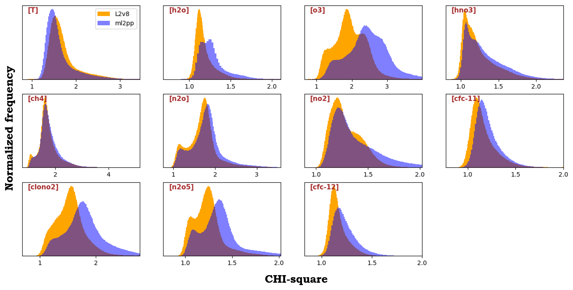
Figure 2 Chi-square distribution of all OR NOM L2 V8 (orange) and L2 V7 (blue) profiles for some representative trace species.

4.1 Model of the horizontal variability

Systematic differences between profiles retrieved from the measurements acquired in the day and the night parts of the satellite orbit were observed, for species for which a diurnal variability is not expected, in the L2 products V7 and earlier. As described in Sect. 2, with the only exception of high-latitude measurements for which the illumination depends on the season, in the MIPAS data set day/night differences are a synonym for descending/ascending differences.

Systematic day/night differences were first noted by Kiefer et al. (2010), who compared zonal averages of MIPAS measurements owing to the ascending and to the descending parts of the satellite orbit. The observed differences are of the order of the retrieval noise error; therefore they are only visible when averages of large data sets are compared. Kiefer et al. (2010) attributed this effect to the missing model of the horizontal variability of the atmosphere within the radiative transfer code. In fact, assuming a linear variation of the atmospheric state parameters with latitude, a given north–south gradient has opposite-in-sign projections along the instrument line of sight, depending on whether the measurement is acquired in the ascending or in the descending part of the orbit. As a consequence, a forward model assuming a horizontally homogeneous atmosphere will simulate radiances affected by opposite-in-sign systematic errors in the ascending and in the descending parts of the orbit. In turn, this forward model error will be mapped into systematic overestimates/underestimates of the mean retrieved profiles in the ascending/descending sections of the orbit. Ascending/descending differences were shown (Kiefer et al., 2010) to vanish when adopting a full tomographic retrieval approach (Carlotti et al., 2001), confirming the need to take into account the horizontal variability. Extensive tests (Kiefer et al., 2010; Castelli et al., 2016) showed that modelling the horizontal variability of the atmosphere with an externally supplied horizontal gradient (HG) could significantly reduce the systematic mean ascending/descending differences, provided that a proper effective gradient estimate is used. According to these results the ORM was modified so that, starting from V8, it models a height-dependent HG of both temperature and gas VMR. HGs are not retrieved; they are computed from external profile databases. The allowed profile data sources are the ECMWF database (see Sect. 4.3.2), results of previous L2 MIPAS/ESA data processing and the IG2 database (see Sect. 4.3.1), which includes the climatological variability with latitude. Sensitivity tests have shown that the HGs determined on the basis of the climatological latitude variability tabulated in the IG2 database do not lead to significant reductions of the ascending/descending differences in the L2 products.

Since the horizontal resolution of MIPAS was of the order of the horizontal separation between the measured limb scans (von Clarmann et al., 2009b), one may argue that atmospheric variabilities at smaller scales should contribute to the individual measurements with a signal smaller than or of the order of the noise. According to this reasoning, we tried to determine effective HG estimates from the differences between profiles retrieved from adjacent MIPAS scans in earlier reprocessing (with the assumption of horizontal homogeneity). These HGs were actually found to reduce markedly the ascending/descending differences in the L2 products. Another estimate of HGs could be determined on the basis of the ECMWF profiles. We associated the closest ECMWF profile in space and in time with each MIPAS limb scan. HGs were then determined from the differences between the ECMWF profiles associated with the adjacent limb scans. The HGs computed with this approach were found to reduce the ascending/descending differences exactly as the HGs determined from previous MIPAS reprocessing. Considering that profiles retrieved in earlier MIPAS reprocessing (V7 and earlier) may sporadically show unphysical oscillations, for the V8 reprocessing we decided to use HGs determined on the basis of the ECMWF data set. Specifically, from the ECMWF data set, we determined the HGs of temperature, H₂O and O₃. The HGs of the other gases were set to zero.

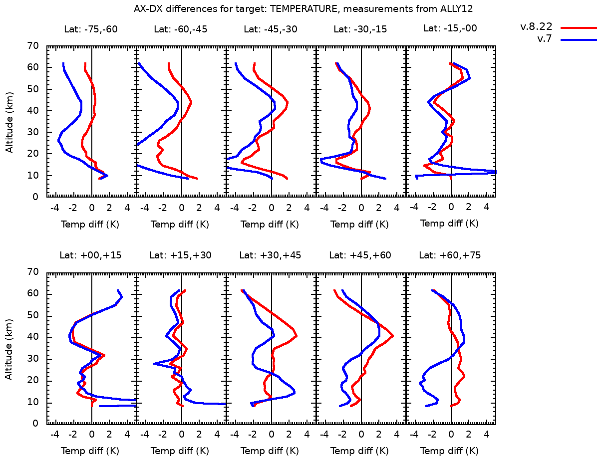
Figure 3 Temperature ascending–descending average difference profiles for V7 (blue) and V8 (red) MIPAS/ESA products. Averaging extends to the measurements acquired in the month of December of the years 2006 to 2011 (OR part of the mission). The different panels show different latitude bands as indicated on the top of the panels.

The HGs are calculated as difference quotients at fixed altitudes along the orbit plane. For each scan, we apply the gradient to the atmosphere up to a distance δOC from the tangent point, where OC (orbital coordinate) is the polar coordinate in the orbit plane. We set δOC as the average inter-scan distance (about 4^∘). Since the actual angular distance between scans differs from scan to scan, corrective actions have been taken to avoid unphysical extrapolations of the atmospheric fields in the OC domain.

Removing the assumption of horizontal homogeneity of the atmosphere implies that Snell's law could not be exploited any longer at the edge of the atmospheric layers, as in the earlier ORM versions. As a consequence, a new ray-tracing algorithm has been developed in order to calculate the Curtis–Godson (Curtis, 1952; Godson, 1953) integrals, defining the equivalent quantities of each layer and allowing for relatively coarse discretisation of the atmosphere (Ridolfi et al., 2000). The new ray-tracing algorithm (Ridolfi and Sgheri, 2014) solves the eikonal equation in Cartesian coordinates using a multi-step predictor–corrector method, with an adaptive step that depends on the curvature of the ray-paths.

Figure 4 CFC-11 ascending–descending average difference profiles for V7 (blue) and V8 (red) MIPAS/ESA products. Averaging extends to the measurements acquired in the month of December of the years 2006 to 2011 (OR part of the mission). The different panels show different latitude bands as indicated on the top of the panels.

Temperature and CFC-11 were identified by Kiefer et al. (2010) as the most critical target parameters, showing the largest ascending/descending differences. Figures 3 and 4 show the average vertical profiles of ascending/descending differences for temperature and CFC-11, respectively. The averaging period covers the measurements acquired in the months of December of the years 2006 to 2011 (i.e. the OR part of the mission). The differences were binned into 10 latitude intervals. We see that, in general, for temperature and CFC-11 the ascending/descending differences in V8 products (red curves) are significantly smaller than in V7 products (blue curves). Specifically, the introduced HG model reduces the temperature systematic differences (by about 1 to 2 K) at mid- to higher latitudes, while preserving the real ascending/descending (night/day) differences at the tropics, due to solar tides.

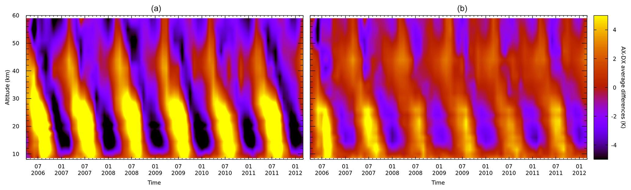
Figure 5 Time series of monthly average temperature ascending–descending difference profiles for V7 (a) and V8 (b) MIPAS/ESA products. The images cover the latitude band from 45 to 60^∘ S.

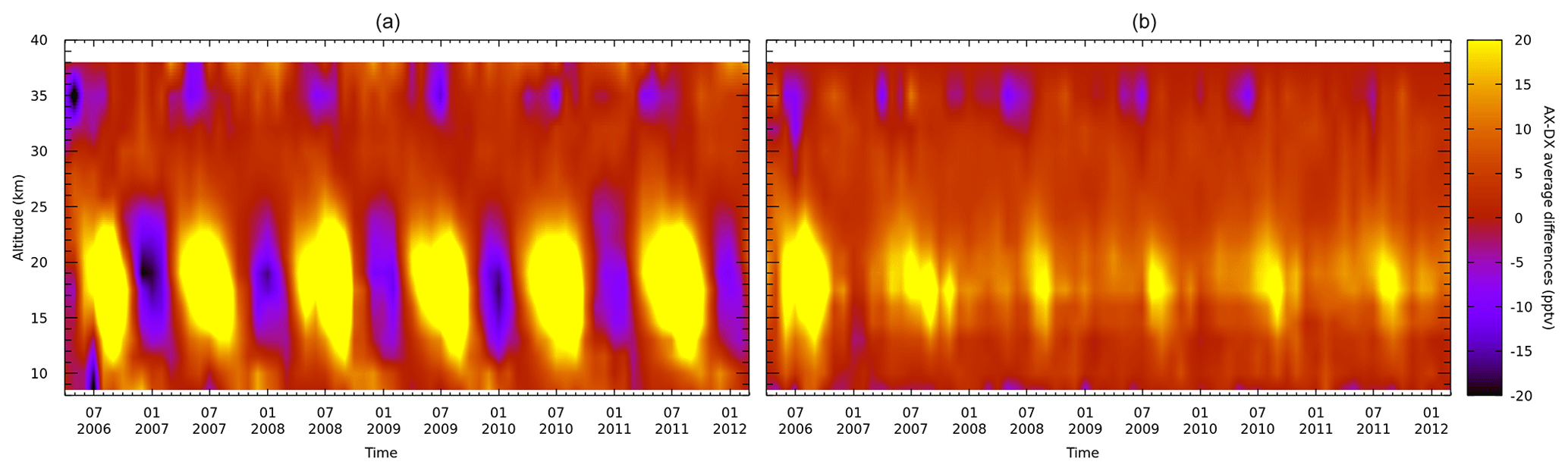
Figure 6 Time series of monthly average CFC-11 ascending–descending difference profiles for V7 (a) and V8 (b) MIPAS/ESA products. The images cover the latitude band from 45 to 60^∘ S.

The systematic ascending/descending differences are linked to the meridional variability of the atmosphere and, therefore, as expected, they depend on the season. The seasonality of these differences is illustrated in Figs. 5 and 6. For a selected latitude band (45–60^∘ S), these figures show the time series of the monthly average temperature (Fig. 5) and CFC-11 (Fig. 6) ascending/descending difference profiles for V7 (left panel) and V8 (right panel). Although still visible, the seasonality of the ascending/descending differences is much less pronounced in V8 data as compared to V7. The remaining seasonality in latitude band averages of V8 measurements could be due to the fact that our model of the horizontal variability of the atmosphere is a first-order model with a gradient, i.e. we only model an inter-scan linear variation of the atmospheric state. Un-modelled smaller-scale atmospheric variabilities, while contributing with a signal below the noise in the individual measurements, could cause a visible effect in the averages.

4.2 Updated spectroscopic data

Full-physics modelling of the measurements requires the knowledge of the spectroscopic parameters of the trace species emitting in the spectral region to be simulated. Indeed, errors in the spectroscopic parameters are estimated to provide one of the major contributions to the total error budget of the retrieved profiles (Dudhia, 2019). The crucial role played by the quality of spectroscopy in the quality of retrieved profiles has motivated the development of a dedicated spectroscopic database for MIPAS with an activity that proceeded in parallel with the development of the L2 processor. For the analysis with ORM V8, the MIPAS dedicated spectroscopic database HITRAN_mipas_pf4.45 was used, which is the evolution of the HITRAN_mipas_pf3_2 spectroscopic database used for the processing of V6 and V7 L2 data sets. The format of the spectroscopic database pf4.45 is compliant with HITRAN 2004.

HITRAN_mipas_pf4.45 is based on HITRAN08 (Rothman et al., 2009), but spectroscopic parameters for the molecules O₂, SO₂, OCS, CH₃Cl, C₂H₂ and C₂H₆ are taken from HITRAN 2012 (Rothman et al., 2012). The spectroscopic parameters of HNO₃ were derived by Perrin et al. (2016), and the spectroscopic data for COCl₂ were derived by Tchana et al. (2015). Both HNO₃ and COCl₂ data are now contained in HITRAN 2016 (Gordon et al., 2017). Spectroscopic data for the new molecule C₃H₈ (Flaud et al., 2010; Nixon et al., 2009), which are not present in the HITRAN data set up to 2016, have been included in the pf4.45 data set. Among the species for which spectroscopic data have changed significantly with respect to the previous MIPAS spectroscopic database, HITRAN_mipas_pf3_2, we have to mention HCN (see Sect. 4.2.2). Spectroscopic line data relative to HOBr are still excluded from the database as the available data are for pure rotational transitions and are outside the MIPAS bands. Line data relative to CF₄ are also still excluded from the database since their quality is very poor.

For molecules which exhibit very dense line-by-line spectra that are extremely difficult to model, or for which the individual transitions have not been assigned, are not accurate enough or are of poor quality, cross-sections measured in the laboratory for atmospheric pressure and temperature ranges are used. It is worth noting that cross-sections also have the advantage of incorporating various spectroscopic effects, such as line coupling and pressure shifts. Measured cross-sections are used for the following molecules: CFC-11, CFC-12, CFC-13, CFC-14, HCFC-21, HCFC-22, CFC-113, CFC-114, CFC-115, CCl₄, ClONO₂, N₂O₅, HNO₄ and SF₆. Among these, new cross-sections have been used in ORM V8 for CFC-12, CFC-14, HCFC-22, CCl₄, ClONO₂, HNO₄, taken from HITRAN 2016 (Rothman et al., 2017), CFC-11 (Harrison, 2018), CFC-113 (Le Bris et al., 2011) and SF₆ (Driddi et al., 2022).

It is important to note that MIPAS measurements themselves were used for some molecules to verify that the new spectroscopic parameters obtained by laboratory measurements allowed for the reduction of the differences between observed and simulated spectral features and, thanks to the broadband spectra of MIPAS, checking of the consistency of the line parameters of a given molecule in its different absorption bands. This is the case for HNO₃, for which an absolute intensity calibration was performed to “convert” the relative line intensities at 7.6 µm to absolute intensities. This was done by comparing the HNO₃ VMR profiles retrieved from the MIPAS radiances in either the 7.6 or 11 µm regions. A multiplicative factor was applied to all the line intensities at 7.6 µm so that in the height range of the HNO₃ VMR peak (21–24 km), the VMR retrieved using the 7.6 µm interval matched the one retrieved using the 11 µm region, leading to better consistency between the 11 and 7.6 µm regions (Perrin et al., 2016).

In Figs. 7, 8 and 9 three examples are shown of spectral intervals selected for the retrieval of HNO₃, COF₂ and CFC-12 VMR, where differences in the residuals come from the changed spectroscopic data only. It is evident that the use of the new spectroscopic database and the new cross-sections significantly reduces the residuals.

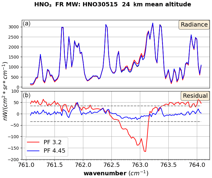
Figure 7 (a) Observed spectrum (black curve, under the blue one) and simulations at a limb tangent height of 24 km with the old (red curve) and the new (blue curve) spectroscopic parameters for a microwindow used for HNO₃ retrieval of FR measurements. (b) Residuals obtained with simulations generated with the old spectroscopic database (red curve) and the new one (blue curve), compared with the measurement noise (grey curves).

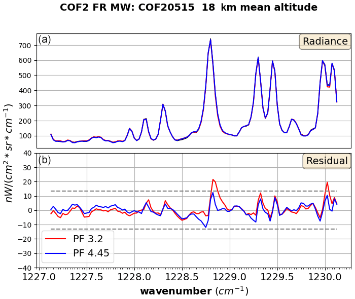
Figure 8 (a) Observed spectrum (black curve, under the blue one) and simulations at 18 km with the old (red curve) and the new (blue curve) spectroscopic parameters for a microwindow used for COF₂ retrieval of FR measurements. (b) Residuals obtained with simulations generated with the old spectroscopic database (red curve) and the new one (blue curve), compared with the measurement noise (grey curves).

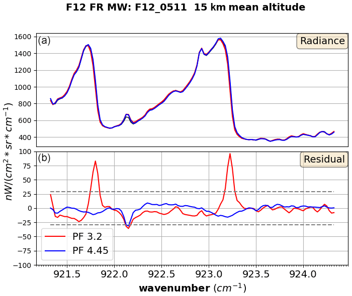
Figure 9 (a) Observed spectrum (black curve, under the blue one) and simulations at 15 km with the old and the new spectroscopic parameters for a microwindow used for CFC-12 retrieval of FR measurements. (b) Residuals obtained with simulations generated with the old spectroscopic database (red curve) and the new one (blue curve), compared with the measurement noise (grey curves).

Impact on retrieved species

We have shown some examples of how the use of the new spectroscopic parameters and cross-sections improves the spectral simulations of the observations, but they also lead to significant changes in the retrieved profiles. The validation of the retrieved profiles is outside the scope of this paper. Here we only describe the impact of the changes in the spectroscopic line data and the cross-sections on the retrieved profiles for the most-affected trace species.

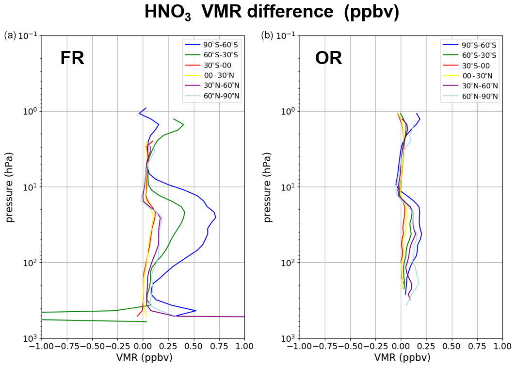
Figure 10 Absolute difference between the mean HNO₃ profiles retrieved using the new (mipas_pf4.45) and the old (mipas_pf3.2) spectroscopic databases at different latitude bands for selected orbits in the full resolution (FR) phase (a) and in the optimised resolution (OR) phase (b).

Spectroscopic line data updates mostly affect HNO₃, HCN and COCl₂. The use of the updated spectroscopic database for HNO₃ causes systematically larger profiles between 100 and 10 hPa, with the largest differences being 0.7 (0.2) ppbv for the FR (OR) measurements around the peak of the profile in the Antarctic region (see Fig. 10), corresponding to differences of about +5 % (2.5 %) for the FR (OR) measurements.

Figure 11 Same as Fig. 10, but for the HCN profiles.

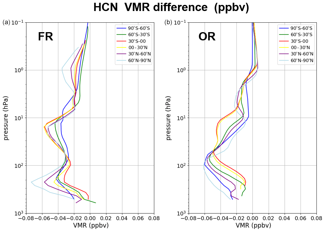
For HCN the changed spectroscopy is responsible for an even larger difference, greater than 20 pptv between 200 and 10 hPa (see Fig. 11), corresponding to 15 %–20 %. The reason is that a major update has been accomplished for the hydrogen cyanide line list since HITRAN 04. Line positions and intensities throughout the infrared have been revisited by Maki et al. (1996, 2000). The improvements apply to the three isotopologues present in HITRAN in the pure rotation region and in the infrared from 500 to 3425 cm⁻¹. The new intensities are about 1.16 times larger than the previous ones.

For the impact of the changes in COCl₂ spectroscopy on the retrieved profiles, we refer the reader to Pettinari et al. (2021).

Systematic differences in the retrieved trace species attributable to changes in the used cross-sections are found in CCl₄, CFC-11, CFC-12 and HCFC-22 retrieved profiles. In general, for all the four trace species the new cross-sections are characterised by a higher spectral resolution and better signal-to-noise ratio at low pressure than the previous ones.

Figure 12 Same as Fig. 10, but for the HCFC-22 profiles.

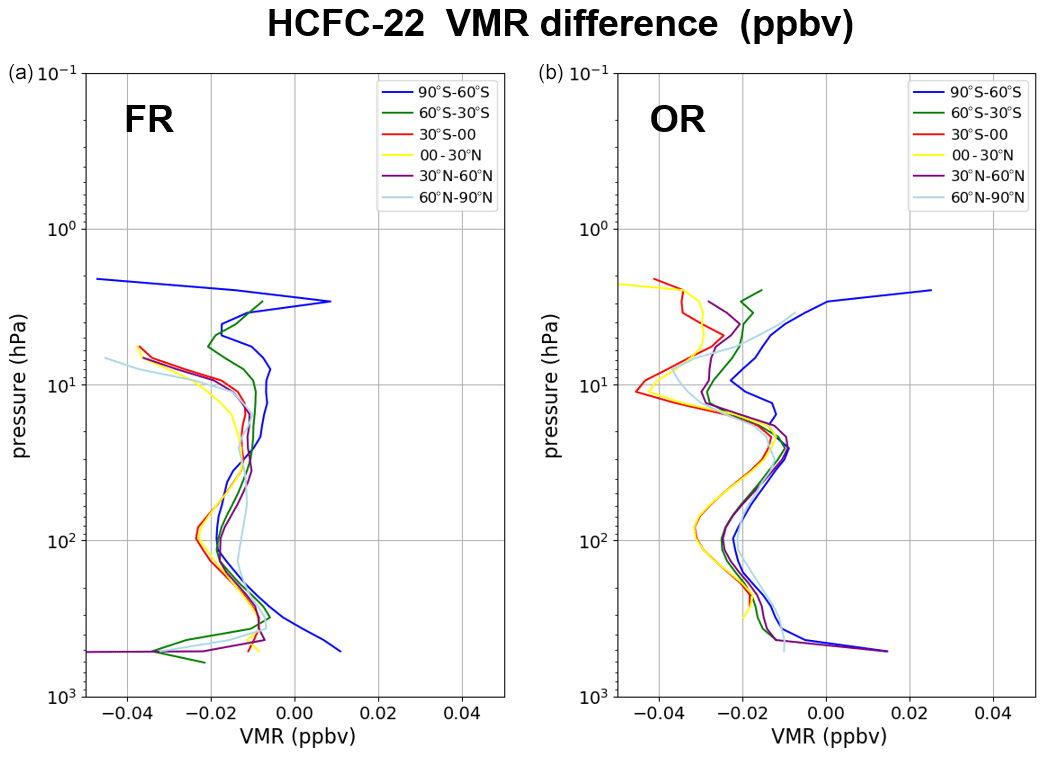
The use of the new cross-sections for HCFC-22 (Harrison, 2016) leads, above 200 hPa, to retrieved HCFC-22 VMRs between 10 and 25 pptv, smaller than with the old cross-sections (Prasad Varanasi, private communication, 2000; Clerbaux et al., 1993; see Fig. 12), corresponding to differences of about 10 %. A possible explanation for this difference is that the Q branches are reasonably sharp, especially near 829 cm⁻¹, and very sensitive to pressure. So even though the overall integrated band strength is the quite similar, differences can be due to the extended pressure coverage of the new cross-sections.

Figure 13 Same as Fig. 10, but for the CFC-11 profiles.

Figure 14 Same as Fig. 10, but for the CCl₄ profiles.

Figure 15 Same as Fig. 10, but for the CFC-12 profiles.

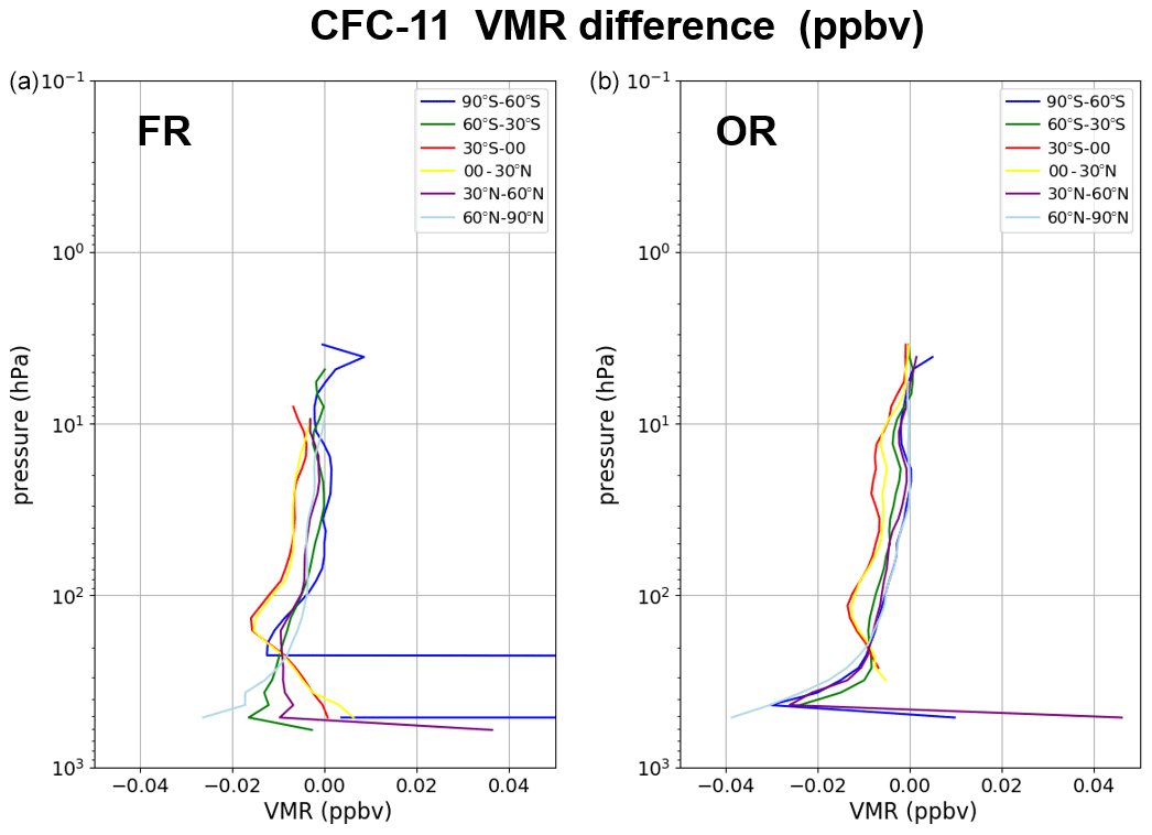
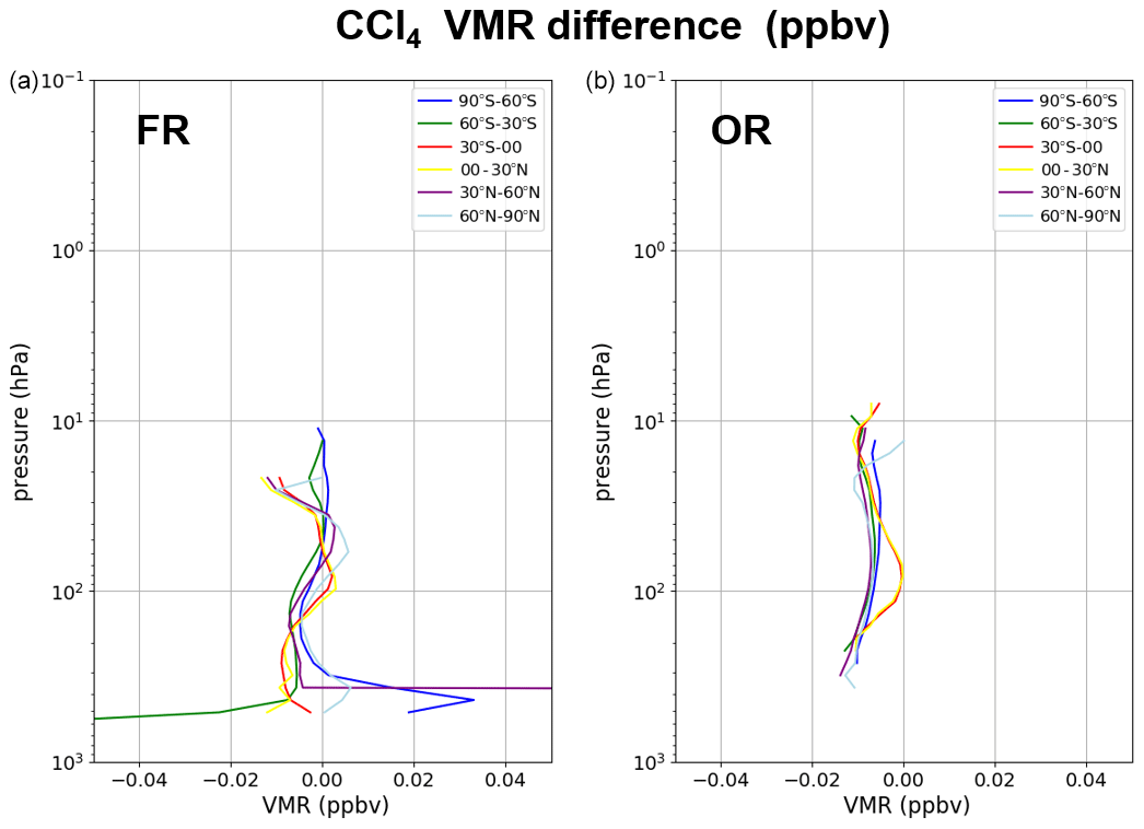
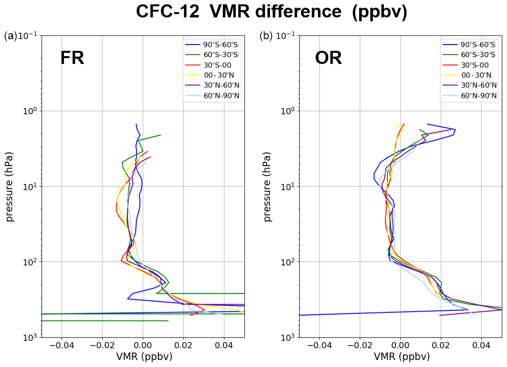
Concerning the other retrieved profiles, V8 CFC-11 VMRs obtained with the new cross-sections (Harrison, 2018) are up to 20–30 pptv smaller than with the old ones (Prasad Varanasi, private communication, 2000; see Fig. 13), corresponding to a percent difference of up to 5 %. Differences in CCl₄ VMRs retrieved with the new (Harrison et al., 2016) and the old (Prasad Varanasi, private communication, 2000) cross-sections vary from very small values at 100 hPa for the tropical bands to −5 to −10 pptv from 200 to 20 hPa for the other latitude bands and altitudes (see Fig. 14). Finally, the new CFC-12 cross-sections (Harrison, 2015) are responsible for an increase in the retrieved CFC-12 profiles with respect to the old cross-sections (Prasad Varanasi, private communication, 2000), which is maximal at the lowest altitudes and equals about 50 pptv; then the difference gradually reduces with altitude, becoming negligible at 100 hPa, and slightly negative above (Fig. 15).

Figure 16 Absolute difference between MIPAS V8 and MIPAS V6 CFC-12 profiles at different latitude bands for selected orbits in FR (a) and OR (b) phases.

For CFC-12, it is interesting to compare the differences in the retrieved profiles between V8 and V6 products with the results of the validation of V6 data with the balloon BONBON measurements (Engel et al., 2016), which uses gas chromatography, for an indirect verification of the improvements implemented in the V8 processor. The use of the new cross-sections, combined with the other changes implemented in the code, produces differences between V8 and V6 of the opposite sign in the two phases of the mission (positive in the OR, negative in the FR; Fig. 16), which compensates for the bias between MIPAS V6 and BONBON measurements (negative in the OR, positive in the FR; see Fig. 13 of Engel et al., 2016) leading to a better agreement.

For the other species validated with the same technique, namely CH₄, N₂O and CFC-11 (Engel et al., 2016), the detected biases of V6 products with respect to BONBON (up to 300 ppbv at 15 km for FR measurements in CH₄, up to 50 ppbv at 15 km for FR measurements in N₂O and up to 40 pptv for CFC-11 in both phases of the mission) were already partially reduced in V7 products thanks to the use of new N₂O and CH₄ microwindows for the analysis of FR measurements and to the handling of the interference of COCl₂ in CFC-11 retrievals (De Laurentis et al., 2016). Furthermore, no significant differences are found in V8 CH₄ and N₂O with respect to the corresponding V7 products, and the effect of the new cross-sections for CFC-11 is smaller than the effect of the unaccounted COCl₂ interference in V6 CFC-11 profiles.

4.3 Use of a priori knowledge of the atmosphere

In order to perform the retrieval, it is necessary to define the initial and a priori state of the atmosphere. The atmosphere is described by the vertical distribution of pressure and temperature, as well as of the VMR of both the retrieval targets and the interfering species, and, with the handling of horizontal inhomogeneities, also of the horizontal (latitudinal) gradients of the considered species. The choice of these profiles, in particular of the ones which are not target of the retrieval, is important, because a wrong assumption may introduce systematic errors in the retrieved quantities. In general, the following databases have been developed for defining the state of the atmosphere.

• The IG2 data set, consisting of a set of climatological profiles of the global atmosphere for six latitude bands, four seasons (January, April, July and October) and for all years of the MIPAS mission in both nighttime and daytime conditions. These profiles are available for all targets and interfering species in the altitude range 0–120 km. The methodology used for generating these data is based on Remedios et al. (2007), and the improvements implemented in version V5.4 (used for the L2 V8 reprocessing) are described in Sect. 4.3.1.

• Profiles from ECMWF ERA-Interim reanalysis that have been chosen for each scan as the closest to MIPAS measurements: this data set includes pressure, temperature, water vapour and ozone profiles in the altitude range 0–65 km. The way they are selected is described in Sect. 4.3.2.

• For the target species, retrieved in sequence from each measured scan, the following profiles can also be used, if available and of “good” quality (see Sect. 6.2): profiles from previous retrievals of the current measurement scan; retrieved profiles from the previous scan; retrieved profiles from previous MIPAS reprocessing.

Among the different databases, only the IG2 profiles are available for the altitude range from 0 to 120 km, the others being defined by a restricted altitude range. The extension of these profiles outside their native range is performed with the IG2 profiles which, in order to avoid discontinuities, are scaled by the ratio between the value of the profile at each edge of its native altitude range and the corresponding climatological value interpolated at the same altitude.

The code uses a priority system to determine the best possible choice for the target species and the interfering species (see Dinelli et al., 2021).

4.3.1 IG2 data set

The IG2 database (Remedios et al., 2020) consists of the climatological profiles for the following six latitude bands: 90 to 65^∘ N, 65 to 20^∘ N, 20^∘ N to 0, 0 to 20^∘ S, 20 to 65^∘ S and 65 to 90^∘ S for the four seasons each represented by its central month January, April, July and October. Profiles are represented on a 1 km step vertical grid from 0 km to 120 km for pressure (hPa), temperature (K) and volume mixing ratios (ppmv) of the following species: N₂, O₂, C₂H₂, C₂H₆, C₃H₈, CO₂, O₃, H₂O, CH₄, N₂O, CFC-11, CFC-12, CFC-13, CFC-14, CFC-21, HCFC-22, CFC-113, CFC-114, CFC-115, CH₃Cl, CCl₄, HCN, NH₃, SF₆, HNO₃, HNO₄, NO, NO₂, SO₂, CO, HOCl, ClO, H₂O₂, N₂O₅, OCS, ClONO₂, COF₂, COCl₂, HDO and PAN. Daytime and nighttime profiles are provided for the trace gas species that display strong diurnal signatures, namely CH₄, ClO, ClONO₂, H₂O, HNO₃, HNO₄, HOCl, N₂O₅, N₂O, NO₂ and O₃. For specific gases (i.e. chlorofluorocarbons and CO₂), trends are accounted for in the IG2 climatology. Although the profiles are tabulated only for a limited set of latitude bands and for each season of the years 2002 to 2012 in the IG2 database, discontinuities in the L2 products are avoided by using linear interpolation. Specifically, for each processed limb scan, the ORM V8 builds the corresponding IG2 profile estimates by linearly interpolating the IG2 tabulated profiles to the time and the geolocation of the considered measurement.

Table 1 Summary of input data for IG2 V5 profiles. For previous versions, we refer the reader to Remedios et al. (2007). The standard atmosphere (SA) database is a set of climatological profiles that represent the global atmosphere under conditions of varying atmospheric state (Remedios et al., 2007). Other data sets used are described in the text.

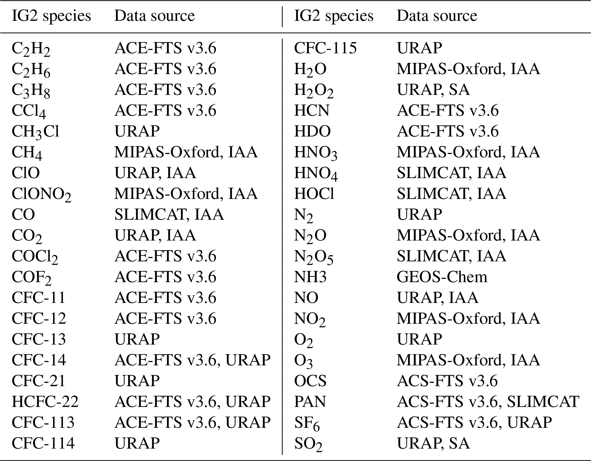
The creation of the IG2 profiles follows the methodology of Remedios et al. (2007), in which several data sources are selected for specific regions of the atmosphere and merged to create a full vertical concentration profile from the ground to 120 km. The following data sets are used for the creation of the V5 IG2 profiles: URAP (UARS Reference Atmosphere Project) profiles (Remedios, 1998), ACE-FTS on SCISAT v3.6 data set (Bernath et al., 2003), SLIMCAT model profiles (see description below), GEOS-Chem model profiles (Bey et al., 2001 and, for NH₃, Molod et al., 2012), IAA profiles derived for upper altitudes and diurnal variations as required for non-LTE calculations (see description below) and mean profiles calculated from ensembles of MIPAS-Oxford profiles (2008–2009) for the MIPAS target species (Dudhia, 2008). A summary of the input data used for IG2 V5 profiles is provided in Table 1. CFCs and organics are constrained by the V3 ACE-FTS data set with further filtering to remove negative volume mixing ratios. Variable smoothing lengths, depending on species and atmospheric lifetime, are required to smooth out small-scale vertical variability.

For the generation of a day and night data set, the creation of V5 differs only so as to incorporate the diurnal differences expected for some species. This is done by changing some of the input data sets to accommodate other data sources that possess day and night variations. In particular, in the lowest altitude range, the diurnal variation from either the University of Leeds SLIMCAT model (see below) or the climatology from MIPAS products were implemented into the V5 profile creation procedure, while the IAA data set (see below) was mainly used above this altitude range. The output results in two profiles created per gas (per season and per latitude band) rather than a single mean profile.

The University of Leeds SLIMCAT model is a 3D stratospheric chemical transport model that calculates atmospheric abundances of a number of chemical species (Chipperfield, 2006). In a combination with TOMCAT, the inclusive TOMCAT/SLIMCAT model calculates the global chemical tracer fields from the surface to 80 km for short-lived chemical species, and steady state and source gases, using meteorological fields from ECMWF. Here, for the stratosphere, vertical transport is calculated by the CCMRAD (Briegleb, 1992) radiation scheme that encompasses the longwave and shortwave radiation domains (from the surface to top-of-atmosphere). Advection of chemical tracers is performed by the Prather scheme (Prather, 1986). A diurnally varying SLIMCAT data set was computed specifically for the creation of IG2 diurnally varying profiles. Chemical calculations were performed on a monthly scale from pre-Pinatubo years to years including ENVISAT coverage (1990–2008), driven by ECMWF reanalysis, and calculated on a 1 km vertical grid extending from the surface to 60 km (1999–2005) and 80 km (2006–2008). The chemical tracers included in these calculations are O₃, O, O(¹D), N, NO, NO₂, NO₃, N₂O₅, HNO₃, ClONO₂, ClO, HCl, HNO₄, HOCl, Cl, Cl₂O₂, OClO, Br, BrO, BrONO₂, BrCl, HBr, H₂O₂, HOBr, CO, CH₄, N₂O, H, OH, HO₂, H₂O, H₂SO₄, CFC-11, CFC-12, CH₃Br, CH₂O, HF, COF₂ and COFCl. Data are provided as zonally averaged day and night concentration profiles, zonal minimum/maximum day and night profiles and standard deviation day and night profiles. Data are gridded onto a 5^∘ latitude grid ranging from 85^∘ S to 85^∘ N and on a 1 km vertical grid.

Climatology from MIPAS products was generated for a check on diurnal variation provided by SLIMCAT. In particular, MIPAS-Oxford profiles (Dudhia, 2008) were used. A Z test filter (Daszykowski et al., 2007) was applied to the MIPAS-Oxford data to remove any outliers. Some control tests performed with ORM, consisting of pressure and temperature retrievals for selected orbits covering the four seasons, performed using the climatological profiles taken from either the V4.1 IG2 database or the new diurnally varying IG2 database as the interfering species profiles, revealed that larger chi-square values were found compared to the V4.1 IG2 database when using N₂O₅ profiles derived by SLIMCAT, with the largest discrepancies in the polar regions. It was found that the N₂O₅ profiles generated by SLIMCAT did not appear to suitably represent the diurnal variation (10:00/22:00) expected for these species, especially in the polar regions, despite good apparent agreement with the twilight occultation observations of ACE-FTS. In the end, mean profiles calculated from ensembles of MIPAS-Oxford N₂O₅ profiles (2008–2009) were preferred over SLIMCAT profiles in defining the diurnal information for generating the V5 IG2 profiles. To keep consistency between all of the diurnal species retrieved by MIPAS, similar V5 IG2 profiles were generated for all operational species (O₃, N₂O, ClONO₂, H₂O, CH₄, HNO₃ and NO₂).

Above 80 km, the IAA data set (López-Puertas, 2009) is mainly used. This supplies a set of climatological profiles extending from the surface up to 200 km for the same six latitude bands, four seasons and nighttime and daytime conditions of the IG2 database. For the generation of these profiles, the SLIMCAT profiles available up to 80 km were extended and/or modified up to 200 km as detailed in Table A1. The data set contains profiles for (a) pressure and temperature, which were taken from the IG database version V4 (Remedios et al., 2007) below 70 km, and from the MSIS model (Picone et al., 2002) above that altitude; (b) VMR profiles for H₂O, CO₂, O₃, N₂O, CO, CH₄, NO, NO₂, HNO₃, OH, ClO, HO₂, O, O(¹D), N, H, N₂, O₂ and HCN; and (c) non-LTE relevant parameters as the photo-dissociation rates of O₂ and NO, $J_{{\mathrm{O}}_{\mathrm{2}}}$ and J_NO, respectively.

To generate this data set, we used a simple 1D chemistry model (the IAA box model), MSIS model (Picone et al., 2002), the 2D model of Garcia and Solomon (1994) and the NOEM (Marsh et al., 2004) for NO. Concerning the diurnal variations, the calculations for particular reference days were performed (see Table 2 in López-Puertas et al., 2009) within the corresponding season (i.e. March–May for April) at 10:00/22:00 local time. These reference days were chosen such that solar zenith angle (SZA) at 10:00/22:00 reflects the average SZA of all MIPAS observations in the corresponding latitudinal and seasonal band in day (SZA < 90^∘) and night (SZA > 90^∘) conditions. The photo-dissociation coefficients, J, were calculated in the IAA box model with the TUV model (Madronich and Flocke, 1998), except for J_NO, which was taken from the Minschwaner and Siskind (1993) parameterisation. More details on the generation of this data set can be found in López-Puertas et al. (2009) and in Sect. 3.1 of Funke et al. (2012).

4.3.2 ECMWF data set

The ECMWF data set is taken from ECMWF ERA-Interim (Dee et al., 2011), the latest global atmospheric reanalysis of ECMWF model results available at the start of MIPAS data reprocessing. The data set covers the period 1979 to 2019 with a spatial resolution of approximately 79 km (T255 spectral) over 60 vertical levels from the surface up to 0.1 hPa. ERA-Interim data include temperature, humidity and ozone profiles, which are made available as 6-hourly atmospheric fields.

Data on model levels were adopted instead of pressure levels in order to obtain a greater vertical coverage since they are released up to 0.1 hPa (about 65 km altitude) versus 1 hPa (about 50 km altitude), respectively. The adoption of levels with a fixed pressure scale implies an inhomogeneous upper limit of the profiles along the orbit. Each MIPAS scan is geolocated assuming vertical alignment of the tangent points of the sweeps at the centre of the scan. In order to obtain the best coincidence between the geolocation of MIPAS scans and ECMWF data, the assignment of ECMWF profiles to each MIPAS scan is performed selecting the ECMWF 6-hourly reanalysis file closest in time to the median scan of the orbit and adopting the model profile at the grid point nearest to the geolocation of the scan. Only one ECMWF file is adopted per orbit, even though the orbit may cross two ECMWF 6-hourly fields; this is to avoid the introduction of spurious gradients passing from one ECMWF file to the following one within the same orbit. The adopted approach avoids interpolation and implies an uncertainty of the coincidence of ± 3 h and ± 0.35^∘ latitude and longitude (< 38 km), which is consistent with typical validation activities.

Since the errors within the time and spatial window of coincidence are homogeneously distributed, this approach does not introduce any bias in the initial guess profiles.

5 Retrieval of minor species

The number of molecules retrieved by the V8 L2 processor was increased with respect to previous processing, adding C₂H₂, C₂H₆, CH₃Cl, OCS, HDO and COCl₂ to the species provided in V7 data set, namely H₂O, O₃, HNO₃, CH₄, N₂O, NO₂, CFC-11, CFC-12, N₂O₅, ClONO₂, COF₂, CF₄, HCFC-22, HCN and CCl₄. The retrieval of the new trace species is made difficult by the weakness of their signal in MIPAS spectra and by the interference of other molecules. For this reason their analysis was only considered in the latest phase with an algorithm containing additional functionalities.

5.1 Optimal estimation approach

For the full exploitation of MIPAS measurements, the retrieval of minor species was considered. For the trace species for which information is limited to a restricted altitude range or particular latitude regions, the regularising Levenberg–Marquardt approach and a posteriori regularisation method may provide insufficient constraint. For this reason the optimal estimation technique (Rodgers, 2000) was introduced for the analysis of these species to avoid unphysical results.

The retrieval equation at the ith iteration was, therefore, modified with the addition of the optimal estimation constraint:

$$\begin{array}{}\text{(1)}& \begin{array}{rl}{\mathit{x}}_{i+\mathrm{1}}=& {\mathit{x}}_i+{\left({\mathbf{K}}_i^{\mathrm{T}}{\mathbf{S}}_y^{-\mathrm{1}}{\mathbf{K}}_i+{\mathbf{S}}_{\mathrm{a}}^{-\mathrm{1}}+{\mathit{\lambda }}_i{\mathbf{D}}_i\right)}^{-\mathrm{1}}\\ & \times \left[{\mathbf{K}}_i^{\mathrm{T}}{\mathbf{S}}_y^{-\mathrm{1}}(\mathit{y}-F({\mathit{x}}_i\left)\right)+{\mathbf{S}}_{\mathrm{a}}^{-\mathrm{1}}({\mathit{x}}_{\mathrm{a}}-{\mathit{x}}_i)\right],\end{array}\end{array}$$

where x_i is the retrieval vector at the ith iteration, x_a is the a priori retrieval vector, F(x) is the forward model, ${\mathbf{K}}_i=\frac{\partial F\left({\mathit{x}}_i\right)}{\partial {\mathit{x}}_i}$ is the Jacobian, namely the derivative of the observations with respect to the quantities to be fitted, S_y is the CM of the observations, S_a is the CM of the a priori profile, λ_i is the Levenberg–Marquardt parameter and D_i is the diagonal matrix with values equal to the diagonal of $({\mathbf{K}}_i^{\mathrm{T}}{\mathbf{S}}_y^{-\mathrm{1}}{\mathbf{K}}_i+{\mathbf{S}}_{\mathrm{a}}^{-\mathrm{1}})$. When the a priori is not considered, ${\mathbf{S}}_{\mathrm{a}}^{-\mathrm{1}}$ is equal to zero and Eq. (1) reduces itself to the formula used for the Gauss–Newton iteration modified with the Levenberg–Marquardt method.

During the iterations, the Levenberg–Marquardt parameter is different from 0, but after convergence is reached, only if optimal estimation has been used, λ_i is set to 0, an additional iteration is done and no a posteriori Tikhonov regularisation is made. As a consequence, the CM and AKM do not have to take into account the Levenberg–Marquardt parameter and are given by

$$\begin{array}{}\text{(2)}& {\displaystyle }& {\displaystyle }\mathbf{S}={\left({\mathbf{K}}_{\text{i\_end}}^{\mathrm{T}}{\mathbf{S}}_y^{-\mathrm{1}}{\mathbf{K}}_{\text{i\_end}}+{\mathbf{S}}_{\mathrm{a}}^{-\mathrm{1}}\right)}^{-\mathrm{1}},\text{(3)}& {\displaystyle }& {\displaystyle }\mathbf{A}={\left({\mathbf{K}}_{\text{i\_end}}^{\mathrm{T}}{\mathbf{S}}_y^{-\mathrm{1}}{\mathbf{K}}_{\text{i\_end}}+{\mathbf{S}}_{\mathrm{a}}^{-\mathrm{1}}\right)}^{-\mathrm{1}}{\mathbf{K}}_{\text{i\_end}}^{\mathrm{T}}{\mathbf{S}}_y^{-\mathrm{1}}{\mathbf{K}}_{\text{i\_end}},\end{array}$$

where i_end indicates the final iteration, with the Marquardt parameter set to zero.

The a priori profile can be either the initial guess profile or a fixed profile, read from an external file, and defined as the average of the climatological profiles of the considered trace species for all the seasons and all the latitude bands. The second option guarantees that the observed variability in the retrieved products comes from the measurements and not from the variability of the a priori profile. Another possibility is foreseen only for the HDO retrieval, namely that the a priori profile can be the H₂O profile, retrieved in the same scan, scaled for the natural isotopic ratio. Indeed, the use of a fixed climatological profile for HDO would be critical due to the fact that the altitude of the hygropause can change significantly according to latitude and season. The a priori of continuum and offset are given by their initial guess, equal to 1 and 0, respectively.

The a priori CM is computed as follows: the diagonal elements of the sub-matrix related to VMR are calculated as a given percentage of the a priori profile plus an absolute error, useful when the a priori profile goes to zero, and hence the constraint would become too strong. The off-diagonal elements of the sub-matrix related to VMR are calculated considering correlations decreasing exponentially with altitude differences, the strength of the correlations being tuned through a given correlation length (typically between 4 and 10 km). The sub-matrices related to the continuum and offset are diagonally calculated with an absolute error respectively equal to 1 / 10 the maximum value of the continuum and 31.6 $\mathrm{nW}({\mathrm{cm}}^{\mathrm{2}}\mathrm{sr}{\mathrm{cm}}^{-\mathrm{1}}{)}^{-\mathrm{1}}$ (equal to the square root of 1000, defined as the typical variability of the offset value retrieved for each microwindow) .

The use of the optimal estimation approach is selectable by input and it has been used only for the retrieval of the following trace species: HCN, CFC-14, COCl₂, CH₃Cl, C₂H₂, C₂H₆, OCS and HDO.

The profile retrieved with optimal estimation is the weighted mean of the information coming from the measurements and the information coming from the a priori, where the weights are given by the inverse of the CMs of the measurements and of the a priori profile, respectively. The result can hence be biased towards the a priori if the CM of the a priori is not sufficiently large. In order to limit the bias, a rather large CM is used for the a priori profile, its error being a percentage not smaller than 80 % of its value. Nevertheless, for some constituents, only a few degrees of freedom are obtained from each retrieval and the a priori contributes significantly to the retrieved profile, so that useful results can only be obtained by averaging several observations. However, taking the mean of many retrieved profiles, each containing the same a priori information, leads to a reduced effective a priori error and the a priori profile no longer satisfies the implicit assumption of being, within the error, a realistic estimate of the real profile.

In the case of a large number of observations the averaging of the profiles is an important and frequent operation and the problem posed by the a priori is the reason why in the early analyses of MIPAS only the major atmospheric constituents, which did not require a priori information for the retrieval, were considered. Meanwhile, a new method, in which the a priori components can be reduced, has been developed for the calculation of average profiles (Ceccherini et al., 2014). This new method removes the downsides of the use of a priori information, provided that information about the used a priori is made available to the users together with the products and the quantities that characterise them (CM and AK). In perspective, the possibility of changing the strength of the constraint in subsequent analyses will establish new requirements for the provision of retrieval products.

5.2 Multi-target approach

In addition to the optimal estimation approach, in the new version of ORM the multi-target retrieval (MTR) functionality (Dinelli et al., 2004), the simultaneous retrieval of two or more species, has been implemented. The MTR functionality was meant to cope with strong contamination of the analysed spectral region by the emission of molecules that are insufficiently characterised. However, the sequential retrieval, the careful selection of the spectral region to be analysed and the use of spectral masks have enabled the reduction of the contribution of the interfering species to the point that the MTR functionality was only used for dedicated analyses and not for the full mission reprocessing of the MIPAS V8 L2 database.

6 Reduction of the outliers

An outlier is a data point that differs significantly from other observations. An outlier may be due either to the real variability of the measurement or it may indicate an error in the measurements (corrupted spectra) or in the retrieval procedure (either too little information in the measurements, which leads to large errors in the retrieved products and to instability of the retrieval due to ill conditioning, or unaccounted effects in the forward model). The challenge is to maintain the first type of outliers and to filter out the others. Considering that the products of a retrieval can be used in subsequent retrievals, it is crucial to assess the quality of the data and perform filtering while avoiding further error contamination. A large effort was dedicated to the reduction of the outliers, preventing the retrieval from becoming unstable, through the use of an updated approach for filtering out cloud contaminated spectra, and after the retrieval, with a more comprehensive method to judge the quality of the products.

6.1 Improved cloud-filtering

Clouds impact the whole MIPAS spectral range with both smooth (cloud continuum) and sharp (line distortions due to scattering) features. Both effects can be observed at the MIPAS spectral resolution (Spang et al., 2004; Greenhough et al., 2005; Höpfner et al., 2006). Spectral signatures of polar stratospheric clouds can also be observed in MIPAS spectra (Höpfner et al., 2018). This means that, while on one hand cloud information can be extracted from MIPAS measurements, on the other hand cloud radiative effects can mask the spectral features of the target gases, strongly affecting their retrieval. As a consequence, limb measurements affected by optically thick clouds must be identified and flagged, so that the retrieval of the trace gases concentration can be performed using only the measurements with tangent heights above the cloud. A cloud detection scheme (Spang et al., 2004; Raspollini et al., 2006) is used to filter out spectra spoiled by clouds. A cloud index (CI) is computed as the ratio of the mean radiance in the 788–796 cm⁻¹ interval, dominated by CO₂ and weak ozone emissions, to the (832–834 cm⁻¹) interval, relatively insensitive to temperature and characterised by aerosols and cloud emissions, as well as some weak ozone and CFC-11 emission lines. Typical CI values for the upper troposphere are CI = 1.8, corresponding to thick clouds; CI = 6.0, meaning no cloud; 1.8 < CI < 4.0, corresponding to clouds of intermediate optical thickness. CI values between 4 and 6 are produced by weaker cirrus clouds such as sub-visible cirrus clouds, or by clouds partially covering the instrument field of view. CIs are computed for all spectra of each scan with tangent heights lower than 44 km. CIs are then examined starting from the highest altitudes, using the tangent altitude of the first spectrum with CI smaller than a given threshold to identify the cloud top height, and removing from the analysis all the limb views below it.

The CI threshold equal to 1.8 used in MIPAS/ESA processing up to V7 is not very effective in filtering polar stratospheric clouds (PSCs). Indeed, unfiltered PSCs were found to be responsible for the presence of outliers in the retrieved H₂O, NO₂ and N₂O₅ for wintertime in the southern polar region. Sometimes the used CI threshold poorly filters high-altitude tropical clouds, thus producing unrealistically large VMRs (e.g. CH₄) in these regions. As expected, on the basis of the increased opacity of the atmosphere due to the presence of clouds, the profiles containing outliers are also characterised by large retrieval errors. Figure 17 shows, as an example, the time series of the monthly mean profiles of H₂O VMRs (upper panel) and of its retrieval errors (bottom panel) for a CI threshold of 1.8. The profiles cover the latitude belt from 60 to 90^∘ S. Outliers are clearly visible in the polar winter of each year between 10 and 60 hPa, where polar stratospheric clouds may occur. Correspondingly, we observe very large retrieval errors, confirming the reduced sensitivity of the measurements due to the opacity of the clouds.

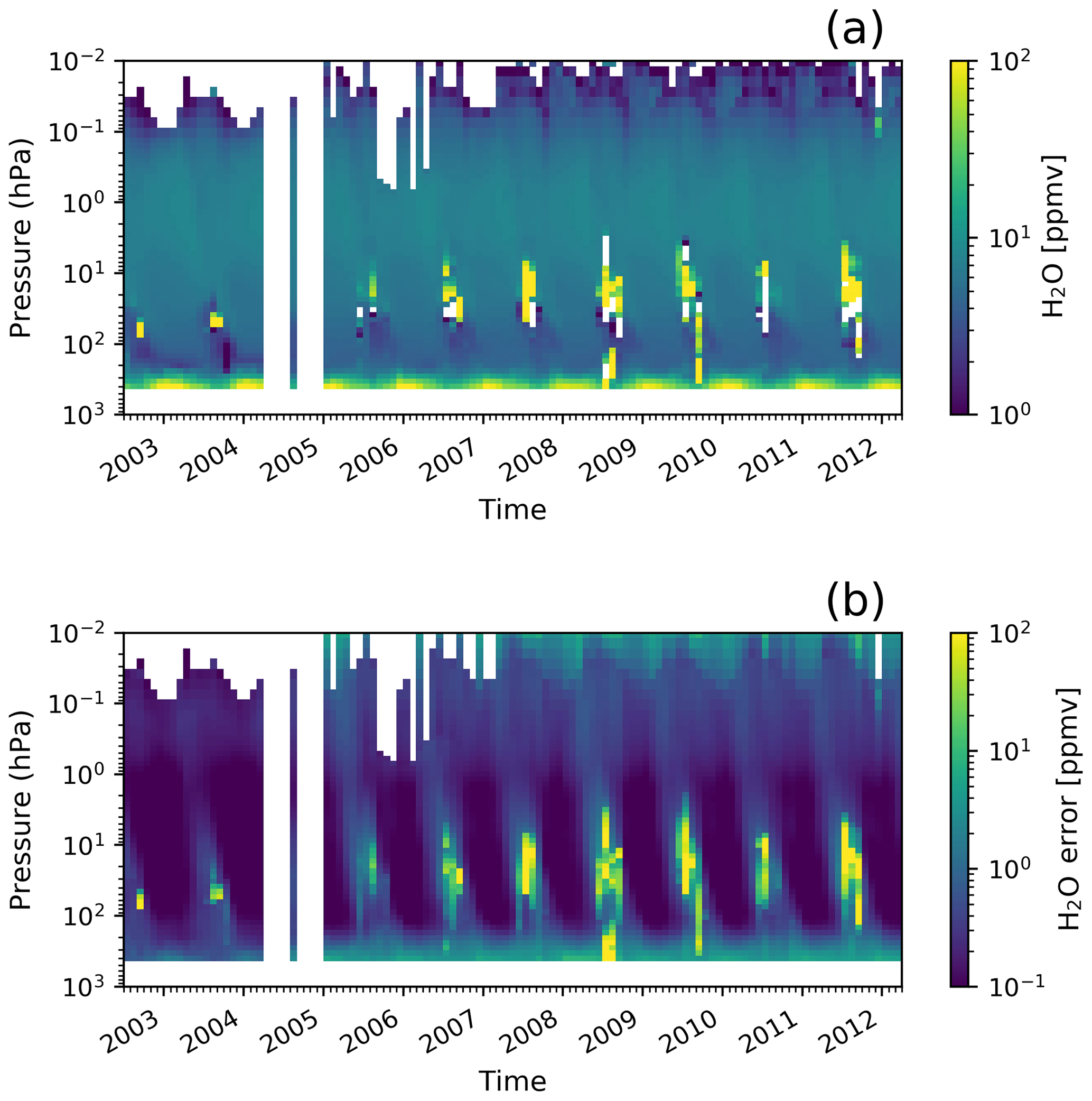
Figure 17 (a) Time series of H₂O monthly mean profiles in the latitude belt from 60 to 90^∘ S and (b) corresponding random error when using a CI threshold of 1.8.

Figure 18 CI profiles computed for all limb scans of orbit 33153 from 3 July 2008. The thicker lines with dots, dark blue and red, respectively, show two selected scans at latitudes 61^∘ S (polar winter), scan number 71, and 63^∘ N (polar summer), scan number 22. The water vapour profiles retrieved from these two scans are shown in Fig. 19.

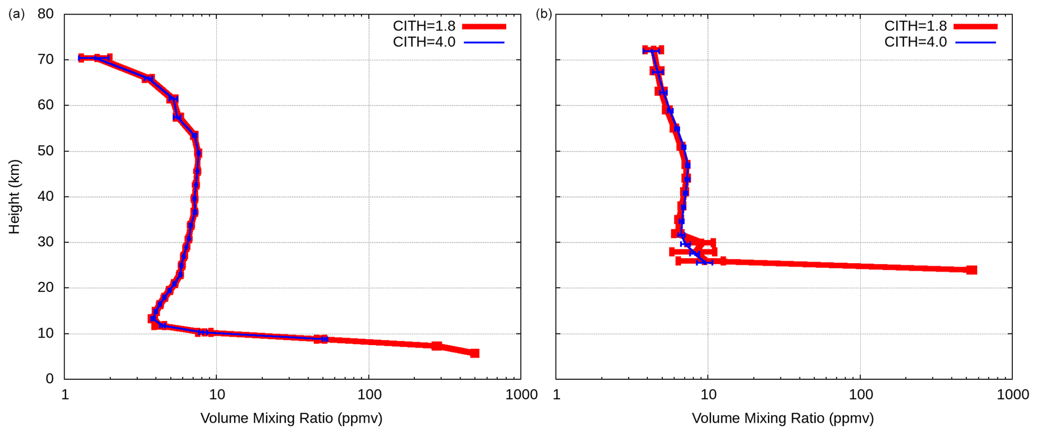
Figure 19 Water vapour profiles retrieved from scan 22 (a, 63^∘ N) and scan 71 (b, 61^∘ S) of orbit 33153 from 3 July 2008. Red profiles are retrieved after filtering the measurements with a CI threshold of 1.8, the blue profiles with a CI threshold of 4.0.

Figure 18 shows examples of the CI profiles computed for all limb scans of orbit 33153 from 3 July 2008. In the same figure the CI threshold of 1.8 (used in the MIPAS/ESA L2 analyses up to V7) and a more conservative value equal to 4.0 (also able to filter out sweeps affected by relatively transparent clouds and used in other independent analyses like Dinelli et al., 2010, and von Clarmann et al., 2009a) are reported. We see that most scans are characterised by CI values larger than 6 above ≈ 26 km. In general, the CI decreases while moving to the lowest altitudes; however, more abrupt reductions are visible in the presence of clouds. In Fig. 18, the two thicker lines with dots (dark blue and red) represent two specific limb scans for which the use of a constant CI threshold for cloud flagging does not produce optimal results. The dark blue line shows scan 71, measured at a latitude of 61^∘ S (polar winter); its CI profiles indicate the presence of a cloud (a polar stratospheric cloud) with a top height around 24 km. Thus all sweeps below this altitude should be excluded from the analysis to safely retrieve good quality VMR profiles. The red line shows scan 22, measured at 63^∘ N latitude (polar summer); in this case the CI profile decreases smoothly when moving to lower altitudes. Therefore, this scan should be classified as clear and all the limb views could be used in the inversion. The water vapour profiles retrieved from scans 22 and 71 are shown on the left and right panels of Fig. 19, respectively. More specifically, Fig. 19 shows the water profiles retrieved from the clear limb views selected using fixed CI thresholds of 1.8 (red profiles) and 4 (blue profiles). From Fig. 19, we clearly see that the threshold of 1.8 is not adequate for scan 71, as it leaves the sweep with tangent height around 24 km unfiltered, responsible for the unrealistically large H₂O VMR at the same altitude (see the red profile in the right panel of Fig. 19). For this scan, the CI threshold equal to 4 performs much better as it correctly filters all the sweeps affected by clouds, thus permitting a reasonable retrieval (see the blue profile in the right panel of Fig. 19). On the other hand, a CI threshold of 4 is too conservative for scan 22 as it erroneously flags as cloudy the two lowest sweeps of the limb scan (see the blue and red profiles in the left panel of Fig. 19). The ORM processor version 8 overcomes these difficulties by using altitude- and latitude-dependent CI thresholds obtained by multiplying the thresholds defined in Sembhi et al. (2012) and Griessbach et al. (2018) by 0.8. The factor 0.8 stems from the fact that the thresholds reported in the above-mentioned papers were developed to derive information on clouds from the measurements, while our goal is only to filter the clouds that significantly impact the retrievals. Examples of CI threshold profiles for polar and tropical latitudes are shown in Fig. 18 with the solid thick blue and magenta lines, respectively. As can be easily seen from Fig. 18, the polar CI threshold profile permits properly flagging the stratospheric cloud that affects scan 71, and retaining all the clear sweeps of scan 22. As expected, the altitude- and latitude-dependent cloud filtering has the effect of significantly reducing the number of outliers in polar winter profiles. Figure 20 is a time series of H₂O monthly mean profiles (upper plot) and errors (bottom plot) retrieved with the ORM V8, from measurements in the 60–90^∘ S latitude belt. Comparing these profiles with Fig. 17, we see how the outliers in both profiles and errors have been removed by the new cloud filtering.

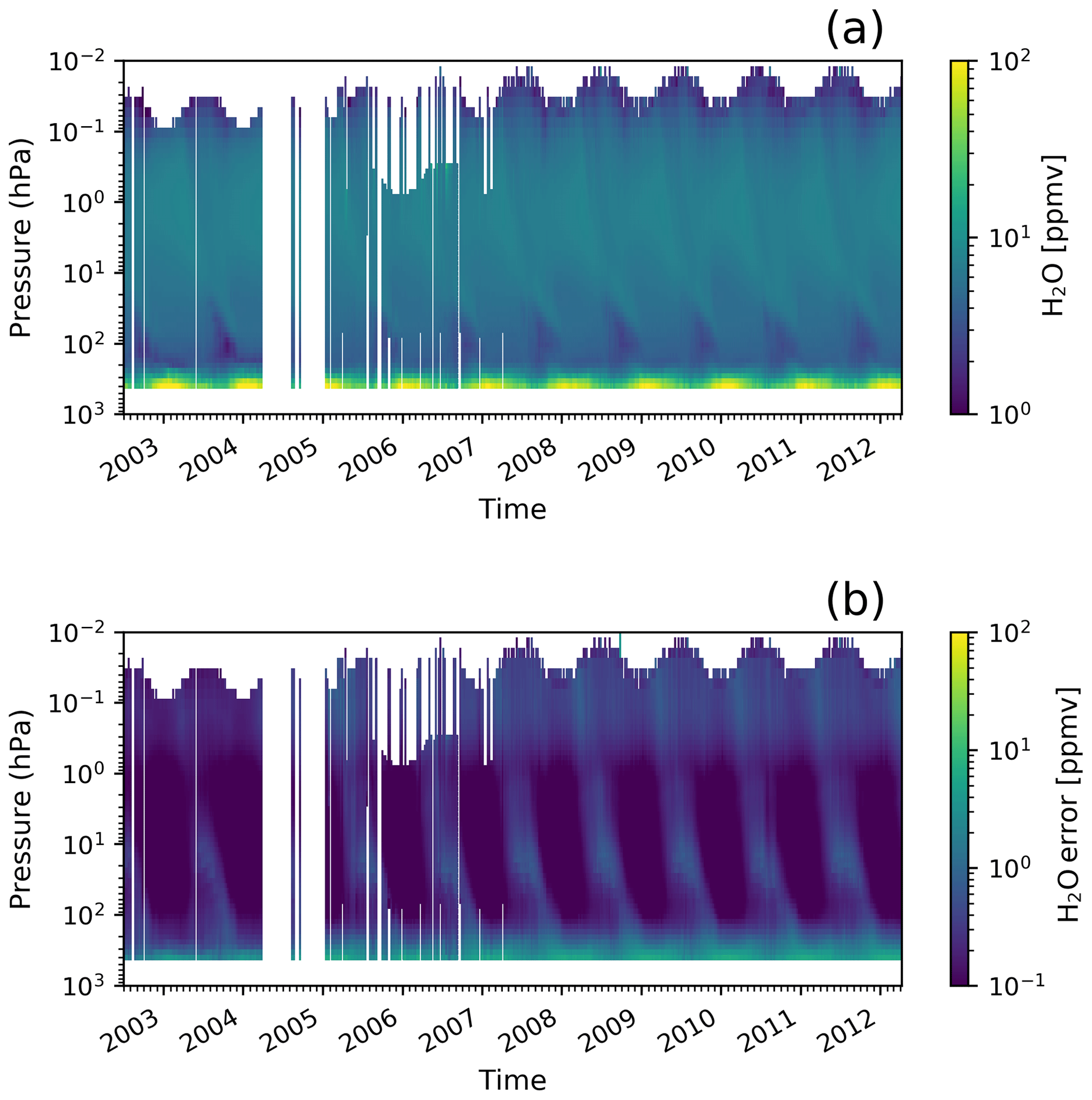
Figure 20 (a) Time series of monthly mean V8 H₂O profiles in the latitude belt from 60 to 90^∘ S and (b) corresponding retrieval error profiles when altitude- and latitude-dependent CI profiles are used.

Table 2 Percentage differences in the number of temperature profile grid points retrieved with the V8–V7 CI thresholds. The statistics are given, separately, for four height ranges and six latitude bands. They include a sample of ≈4000 orbits acquired in nominal (both FR and OR) and UTLS-1 modes.

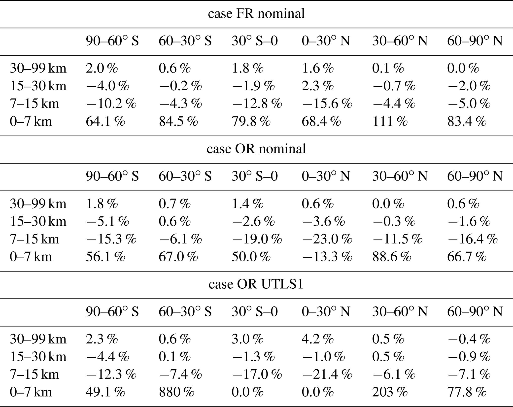
With the new altitude- and latitude-dependent CI thresholds, the statistics of the number of retrieved profile grid points changes with respect to Level 2 V7 products. Table 2 shows the percentage variation (V8 vs. V7) in the number of retrieved temperature profile grid points for different heights and latitude ranges. The statistics reported in the table are based on a sample of ≈ 4000 orbits of nominal (NOM) and UTLS1 measurements of both FR and OR mission phases. The increased number of V8 retrieved data points above 30 km arises from the fact that the a posteriori filtering (see Sect. 6.2) actually removes a smaller number of profiles containing outliers. In the intermediate range, from 7 to 15 km the V8 cloud masking strategy seems far more effective than that of V7, especially in polar and tropical regions. At the lowest altitudes, the new cloud filtering is less conservative than in the V7 data set, and thus, the number of retrieved profile points is greater in the V8 data set.

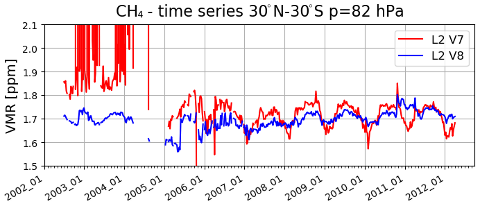
Figure 21 Time series of CH₄ monthly mean profiles in the Tropics, at the pressure level of 82 hPa generated with MIPAS ESA L2 V7 products (red curve) and L2 V8 ones (blue curve).

Errera et al. (2016) found a very poor agreement between MIPAS V6 and V7 products and colocated products of MLS and ACE-FTS, especially in the tropical lower stratosphere. Since the discrepancies were mainly due to MIPAS outliers, we expect improved agreement when the V8 data set are considered. As an example, Fig. 21 compares the V7 and V8 time series of the tropical CH₄ VMR monthly means at the pressure level of 82 hPa. As we can see, the V7 data set contains many outliers, especially in the FR part of the mission, that are no longer present in the V8 data set. In some cases the outliers in the V7 data also hide the seasonal variation of the target parameter considered. This seasonality is now correctly represented in V8 data.

6.2 Quality flagging

In the previous section we have discussed how, by better filtering out spectra affected by clouds, it is possible to reduce the number of outliers in the retrieved profiles. However, outliers can also be the result of problems due to the presence of corrupted spectra or to problems in the iterative retrieval procedure. These can be identified through a quality control of the products performed after the retrieval. In order to avoid any bias in the averages of the retrieved profiles, no constraints are imposed on the values obtained at the end of the retrieval procedure. The quality of the retrieved profiles is judged “good” when three requirements are met: the retrieved profile adequately reproduces the measurements (judged using the reduced chi-square), there are no outliers in the retrieval error and the iterative retrieval procedure successfully converges.

The first condition is met when the chi-square value at the final step of the iterative procedure is smaller than a pre-defined mode and species-dependent threshold. The chi-square provides a measure of how well the results of the retrieval are able to reproduce the measurements within the measurement errors. In the absence of any systematic error or retrieval instability, the spectral residuals should be within the measurement noise level and the expected value of the reduced chi-square equals 1. Although a high chi-square does not necessarily imply that the retrieved quantities are not realistic, exceptionally high chi-square values were found to be associated with bad quality profiles.

The second condition of retrieval errors is met when the maximum value of the retrieval error profile is smaller than a pre-defined mode and species-dependent threshold: indeed, it has been found that there is correlation between outliers and very large retrieval errors.

The third condition is met when the convergence of the Gauss–Newton iterative procedure is attained. This happens if at least one of the following criteria is verified.

• The relative variation of the chi-square between two consecutive Gauss iterations is smaller than a pre-defined threshold (set to 0.01). This is verified in the large majority of the scans.

• The weighted L² norm of the difference between the vector of the retrieved profiles at two consecutive iterations, normalised with the number of retrieved points of the profiles, is smaller than a given threshold. The weight is given by the inverse of the CM of the retrieved parameters. This guarantees that convergence is reached when the retrieval parameters do not change even if there is some variation in the chi-square. The threshold is set to 0.1 for the p, T retrieval, and 0.08 for the VMR retrievals. Only a small number of cases fulfil this criterion.

On the other hand, the retrieval iterations are stopped and convergence is not attained if one of the following two conditions is verified: the maximum number of Gauss iterations (set to 15) is reached; the maximum number of consecutive Marquardt micro-iterations (set to 5) is reached. We face the latter condition when, even with a large Levenberg–Marquardt parameter, no reduction of the chi-square is possible. The successful convergence also requires that the final value of the Marquardt parameter is smaller than a given threshold. Indeed, a too large value of the Marquardt parameter, even if properly taken into account for the computation of the CM and AKM, implies a very small retrieval step, and hence it may trigger false convergence.

When at least one of the previous requirements is not verified, the retrieved profile is flagged as bad in the output file (post_quality_flag=1) and it is not used as either profile of an interfering species or initial guess in subsequent retrievals. Otherwise, if all previous conditions are verified, the post_quality_flag is set to 0 so that the retrieved profile is considered “good” and it can be used for subsequent retrievals. If the retrieved temperature is flagged as bad, no VMR retrieval is performed, since a proper temperature profile is fundamental for the retrieval of the trace species (the cause of the missing VMR profile in the output files can be deduced by the temperature profile flag). The retrieved profiles of some minor species (namely COF₂, CCl₄, CF₄, HCFC-22, C₂H₂, CH₃Cl, COCl₂, C₂H₆, OCS and HDO) are not used in the subsequent retrievals of the chain even if the quality of the products is “good”. This choice was based on a prudence principle, considering that the improvements coming from taking the interference of these trace species in other retrievals are very small, while the presence of possible outliers may negatively impact the retrievals.

The thresholds for the chi-square and maximum error for each species and measurement mode were defined a posteriori using the results of the analyses performed on the so-called diagnostic data set. This consists of about 4000 orbits, e.g. about 1 / 10 of the orbits of the full mission, selected to cover the whole mission period coinciding with most of the correlative measurements used for validation.

Figure 22 shows as an example the chi-square distribution of p, T V7 retrievals relative to the FR phase. The percentile level (Lx) of the distribution, with 0 < x < 100, is determined as the value of the sample such that x % of the total number of samples is less than the Lx. The value of chi-square corresponding to the maximum of the histograms has been labelled as “Hmax”. The criteria used to define the thresholds have been chosen empirically to try to satisfy the two conflicting requirements of both filtering out the largest number of outliers and not throwing away “good” profiles. Considering the different shape of the distributions of chi-square and errors, the values of the thresholds for each product have been then determined using different values of percentile as follows:

$$\begin{array}{ll}{\displaystyle }& {\displaystyle }\text{CHI-square\_threshold}=\mathrm{L}\mathrm{99}+(\mathrm{L}\mathrm{99}-\text{Hmax})\cdot \mathrm{0.5},\\ {\displaystyle }& {\displaystyle }\text{MaxError\_threshold}=\mathrm{L}\mathrm{95}+(\mathrm{L}\mathrm{95}-\text{Hmax}).\end{array}$$

Figure 22 Example of chi-square distribution and considered statistical levels.

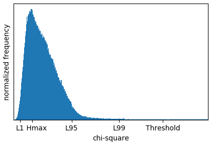
The chi-square distribution is reported in orange in Figs. 1 and 2 for some species considering all the profiles retrieved from the nominal measurement mode, respectively for the FR and the OR phases of the mission. The full-scale value of the x axis is given by the selected threshold. It is evident that only the very far right tail of the distribution is filtered out. The distributions of V7 products are overlapped in blue for comparison. The maximum error distribution (not shown) has a similar shape as the chi-square distribution.

The used thresholds for chi-square, maximum error and final Marquardt parameter are given in the output NetCDF files (see Dinelli et al., 2021).

7 Improvements in temporal stability of the measurements

Ten years of measurements may be a short period to derive atmospheric trends, but they certainly can be used to study the long-term evolution of many species. Furthermore, these measurements can be used in combination with measured data from other sources. To be able to study the time evolution of the species that can be retrieved from MIPAS measurements with high accuracy requires a very stable instrument and careful elimination of any instrumental drift. V8 of the L1b processor (Kleinert et al., 2018) includes several improvements, compared to earlier versions, that have an impact on the temporal variation of the retrieved products. The impact of these improvements to the L2 products has been analysed.

7.1 Improvements in the non-linearity correction

The MIPAS photoconductive detector channels A1/A2, B1/B2, measuring the longest wavelengths, show a non-linear response to the incident photon flux, which has to be taken into account by the L1 processor prior to radiometric calibration. This can be done only if the non-linearity (NL) curve, representing the detector response (voltage) as a function of the incident photon flux, is available. NL correction parameters measured on ground before launch were applied to all measurements up to L1b V5 products. During the mission, in order to reveal possible changes in the NL and to improve its characterisation, dedicated measurements were acquired. The analysis of the in-flight characterisation measurements revealed that, because of the ageing, the photoconductive detectors response slowly decreases, and the detectors become more linear over time. Moreover, the characterisation showed that the NL detector curve depends on the instrument temperature and on the degree of ice contamination (Birk and Wagner, 2010). As a consequence, new parameters for the NL correction were determined from in-flight characterisation measurements. The various upgrades implemented in the NL correction parameters have an impact on the L1b products, which in turn affect the L2 products and in particular the trends that may be derived from these. Figure 23 shows the impact of the NL correction on the retrieved temperature values at specific pressures and different times during the mission. 14 couples of L1b orbits selected to cover the whole mission were created, where the only difference is the NL correction. The differences between the orbit averages of temperature values retrieved from each couple of L1b products are reported for four pressure levels (100, 10, 1 and 0.1 hPa) as a function of the orbit measurement time. We clearly see that the impact of the NL correction on the retrieved temperature varies with altitude (and is significantly larger between 10 and 0.5 hPa) and is negligible at the beginning of the mission; the slope of the temporal variation is relatively steep in the first 5 years of the mission (about 0.1 K yr⁻¹ in the stratosphere) and smoother in the second half of the mission.

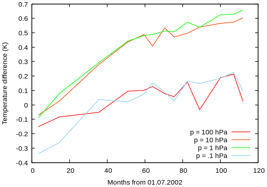
Figure 23 Time dependence of the difference between orbit average temperature values, at the four pressure levels indicated in the key, retrieved (with the ORM V8) using L1b products with and without the NL correction implemented. 14 selected couples of L1b products (from October 2002 to October 2011), generated for this purpose, were used.

A comparison of the MIPAS instrument drift for different versions of the MIPAS L2 products, computed relative to radiosonde and lidar, is presented by Hubert et al. (2020). According to their Fig. 33, a significant reduction in temperature drift between 500 and 0.1 hPa is found for version V8 data in the OR period. A small residual positive drift of at most 0.4 K per decade below 10 hPa still remains. The residual drift can be explained by the uncertainty of the NL correction, mainly due to the fact that the measurements for its characterisation are sparse (only 35 orbits are available throughout the whole mission) and, even more importantly, the continuum level of the signal, which is needed to place the measurements correctly on the NL detector curve, is not provided and has to be estimated from the measured AC-coupled interferogram. The residual uncertainty of the time dependency of the radiometric error has been estimated to be less than 0.5 % per decade (see Fig. 11 of Kleinert et al., 2018). It has to be noted that this uncertainty may have a different impact on the various trace species due to the different spectral intervals selected for the analysis; indeed, species with spectral features in the bands at the lowest frequencies could be more affected by the NL problem. Note, however, that VMRs are retrieved assuming the temperature profile retrieved from the same measurement. This implies that the NL-induced error on the retrieved temperature profile may compensate for the NL error in the subsequent VMR retrievals.

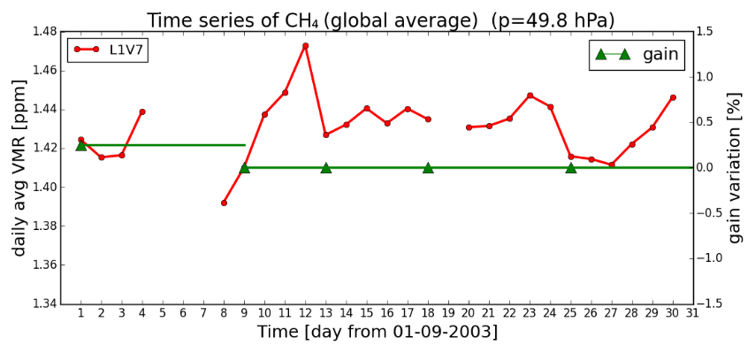
Figure 24 Time series of CH₄ global average at pressure 49.8 hPa relative to September 2003 derived from L2 V7 MIPAS data (red line) and the used gain function (green line), with the triangles indicating the days at which the gain function has been updated.

7.2 Improved gain calibration

Errera et al. (2016) reported discontinuities up to 7 % in the time series of the daily means of both V6 and V7 CH₄ and N₂O MIPAS data, occurring shortly after the decontamination periods. Decontamination consists of a warming of the instrument to remove ice from the mirrors. The discontinuities in the time series of CH₄ and N₂O were found to be correlated with unexplained abrupt changes of up to 2 % in the gain of band B (Kleinert et al., 2018), where the spectral lines of CH₄ and N₂O used for the retrieval are located.

The calibrated radiance is given by the product of the observed scene with the radiometric gain. Before this operation, the observed scene is corrected, subtracting the deep space measurement closest in time in order to take the self-emission of the instrument into account. The gain is determined from a series of blackbody and deep space measurements on a daily basis. However, prior to L1b V7 products, the gain function used for radiometric calibration was updated only once per week. Indeed, the gain variation was usually sufficiently slow so that the error introduced by the temporal drift of the gain function was expected to be small, and weekly averages were chosen to reduce the noise error on the calibration. However, if the gain changes in a timeframe of 1 or 2 d and if the radiometric calibration is not performed on the corresponding days, a discontinuity in the radiance occurs that translates into a discontinuity in the time series of the retrieved products. It has been proven with dedicated tests that, since the relation between the measured radiance and retrieved profile is not linear, a change of 2 % in the gain can induce a change of up to 7 % in the retrieved profile of CH₄, as found in the time series. V8 L1b products were generated with gain measurements updated every day; this allows better capture of the gain variation and hence reduction of the discontinuities in the VMR time series.

Figure 25 Time series of CH₄ global average at pressure 49.8 hPa relative to September 2003 derived from L2 V8 MIPAS data (blue line) and the used gain function (green line), with the triangles indicating the days at which the gain function has been updated.

Figure 24 shows in red the CH₄ global average time series for September 2003 derived from L2 V7 MIPAS data at pressure 49.8 hPa. The used gain function is also reported, in green, with the triangles indicating the days at which the gain was updated (approximately once per week). A large discontinuity occurs from 9 to 13 September 2003 in the CH₄ VMR. Figure 25 reports in blue the same CH₄ global average time series derived from L2 V8 MIPAS data and in green the corresponding gain values, which were updated daily. We see a strong variation in the gain in the period 9 to 13 September, which had been completely masked by a weekly sampling of the gain. The handling of the gain variation allows for the significant reduction, in the L2 V8 data, of the discontinuities which were present throughout the mission in the time series of V6 and V7 CH₄ and N₂O MIPAS data.

8 New format for L2 products

The format adopted for the output files of MIPAS L2 V8 data set is netCDF-4. Two different kinds of files are released: a standard file and an extended one. The decision to provide two output files was driven by the need to make their use easier and to differentiate between information that is needed by most users and information that is needed to undertake diagnostics of the products and for special analyses. Each standard file provides all the information that is generally needed for validating and exploiting MIPAS L2 products. Each file refers to a single orbit and to either a single trace species or to temperature: it contains, for each scan of the orbit, its geolocation and the retrieved profile with the related CM and AKM, as well as used altitude, pressure and temperature profiles and their errors. The quality flags are also available for filtering out bad profiles. The temperature file also contains, as additional information, the cloud index profile, from which it is possible to deduce the cloud top height, as the altitude below the lowest tangent altitude included in the analysis. The main difference in the content of the standard and the extended files is that the extended file provides the full state vector and its related CM and AKM. The full state vector contains, in addition to the retrieved profiles (either VMR profile or pressure and temperature profiles), the atmospheric continuum profiles and instrumental offset. This information is useful when undertaking data fusion (Ceccherini et al., 2015). The size of the files varies with species and observation mode, since it depends on the number of fitted parameters. On average the size of a standard file is about 1 MB, while that of an extended file is about 3 MB. Further information is provided in Dinelli et al. (2021).

9 Conclusions

The new version of the MIPAS ESA L2 processor ORM V8 allows for the retrieval of the temperature profile and the VMR profiles of 21 trace species: water vapour, ozone and many other longer-lived greenhouse gases (CH₄, N₂O, CFC-11, CFC-12, CF₄, CH₃Cl and CCl₄), nitrogen and halogen species of interest for ozone chemistry (ClONO₂, COF₂, N₂O₅, COCl₂, NO₂, N₂O₅ and HNO₃), sulfur compounds (OCS), species contained in biomass burning and other pollution plumes (HCN, C₂H₂ and C₂H₆) and isotopologues (HDO).

The L2 processor ORM V8 and its auxiliary data are significantly different than the ESA L2 processor ML2PP V7. The radiative transfer model was improved by allowing for a linear variation of the atmospheric state (with a gradient) to approximate the actual horizontal variability of the atmosphere sounded by the instrument line of sight. Horizontal gradients computed from ECMWF ERA-Interim reanalysis were assumed in the ORM V8 processing. This improved model implied a significant reduction of the ascending–descending differences that, initially, were erroneously attributed to day/night differences in profiles that are actually not affected by diurnal variability.

The minor species (HCN, CF₄, COCl₂, C₂H₂, C₂H₆, CH₃Cl, HDO and OCS) were retrieved with the optimal estimation method, allowing for stable retrievals also when using large a priori errors.

A better modelling of the measurements was also obtained through the use of improved spectroscopy. The HITRAN_mipas_pf4.45 spectroscopic database (Flaud, 2020) was finalised for this full mission reprocessing. This contains spectroscopic data from different versions of HITRAN databases, data validated with MIPAS measurements themselves (and now contained in HITRAN 2016) and new data. For the heavy molecules, new cross-sections were used by ORM V8 for the following molecules: CFC-12, CFC-14, HCFC-22, CCl₄, ClONO₂, HNO₄, CFC-11, CFC-113 and SF₆. In general the use of updated spectroscopy leads to a better representation of the observations, with smaller differences between observations and simulations, and to significant changes in some retrieved products (HCN, HNO₃, CCl₄, CFC-11, CFC-12 and HCFC-22).

A large effort was dedicated to the representation of the atmosphere, needed for defining the initial guess of the retrieval state vector, the interfering species, the horizontal gradients and the a priori profiles for trace species retrieved with optimal estimation. Even if the highest priority is given, for the choice of the initial guess and interfering species, when available, to the previously retrieved profiles in the same or previous scan, different databases were fine-tuned for the different scopes and used by the retrieval code according to a priority list. The IG2 V5.4 database represents an evolution of the database IG2 V4.0 described in Remedios et al. (2007), and includes climatologies of the daytime and nighttime atmosphere from 0 to 120 km for numerous species. The ERA-Interim ECMWF data set was also used, after the identification of the closest coincidences for each MIPAS scan, for computing the horizontal gradients of temperature, water vapour and ozone. The improved modelling of the measurements was proven by a significant general reduction of the chi-square values for most of the species.

The cloud filtering, used to filter out spectra corrupted by clouds, is in this version altitude- and latitude-dependent and this improves the sensitivity to the presence of clouds. The use of these new thresholds allowed for filtering out spectra affected by polar stratospheric clouds, significantly reducing the number of outliers in water vapour and N₂O₅ retrieved profiles during the polar winter. In general the use of these altitude- and latitude-dependent thresholds reduced the number of retrieved points in the UTLS, but increased the number of retrieved values below 15 km and above 30 km.

Other improvements in the V8 L2 products are a consequence of the reduced instrumental drift and of the use of measured daily gain which reduces the discontinuities in the time series of some species. Output files are provided in NetCDF and contain the L2 products as well as all characterising quantities (CM and AK), and only a flag is needed to filter out low quality products. This flag takes into account various qualifiers which have been further refined and takes into account successful convergence of the retrieval iterations, the capability of the retrieval to reproduce the measurements and the presence of outliers in the retrieval error. The description of the implemented improvements is meant to better explain the products of the ESA L2 V8 reprocessing (which are further characterised in terms of spatial coverage, retrieval errors, spatial resolution and “useful” vertical range considering the whole L2 V8 data set in Dinelli et al., 2021) and also to help the developers of retrieval codes.

Appendix A: The IAA data set

Garcia and Solomon (1994)Garcia and Solomon (1994)Garcia and Solomon (1994)Garcia and Solomon (1994)Garcia and Solomon (1994)Garcia and Solomon (1994)Garcia and Solomon (1994)

Table A1 Summary of the changes introduced in the SLIMCAT output to generate the IAA data set.

^a Picone et al. (2002). ^b Marsh et al. (2004). ^c Log-smoothing with a vertical length of 5 km has been applied to remove unphysical oscillations in the original profiles. ^d NO₂ and NO from the SLIMCAT model were modified below 80 km in order to account for the NO_x descent in the polar regions. Outside the polar regions the SLIMCAT model and the Garcia and Solomon (1994) and IAA box models give very similar values.