Estimating oil sands emissions using horizontal path-integrated column measurements

Improved technologies and approaches to reliably measure and quantify fugitive greenhouse gas emissions from oil sands operations are needed to accurately assess emissions and develop mitigation strategies that minimize the cost impact of future production. While several methods have been explored, the spatial and temporal heterogeneity of emissions from oil sand mines and tailings ponds suggests an ideal approach would continuously sample an area of interest with spatial and temporal resolution high enough to identify and apportion emissions to specific areas and locations within the measurement footprint. In this work we demonstrate a novel approach to estimating greenhouse gas emissions from oil sands tailings ponds and open-pit mines. The approach utilizes the GreenLITE^™ gas concentration measurement system, which employs a laser-absorption-spectroscopy-based, open-path, integrated column measurement in conjunction with an inverse dispersion model to estimate methane (CH₄) emission rates from an oil sands facility located in the Athabasca region of Alberta, Canada. The system was deployed for extended periods of time in the summer of 2019 and spring of 2020. CH₄ emissions from a tailings pond were estimated to be 7.2 metric tons per day (t/d) for July–October 2019, and 5.1 t/d for March–July 2020. CH₄ emissions from an open-pit mine were estimated to be 24.6 t/d for September–October 2019. Uncertainty in retrieved emission for the tailings pond in March–July 2020 is estimated to be 2.9 t/d. Descriptions of the measurement system, measurement campaigns, emission retrieval scheme, and emission results are provided.

1 Introduction

Oils sands are a natural combination of sand, water, clay, and bitumen – a viscous hydrocarbon mixture – that are a source of unconventional petroleum and can be refined to produce crude oil. The largest known deposits of oil sands exist in Canada and Venezuela, with lesser deposits in Kazakhstan and Russia (Tong et al., 2018). Significant deposits of bitumen exist in the Canadian province of Alberta to include the Athabasca, Cold Lake, and Peace River regions (Vigrass, 1968; Mossop, 1980; Hubbard et al., 1999). While all three regions are suitable for production using in situ “drilling in place” methods, such as cyclic steam stimulation (CSS) or steam-assisted gravity drainage (SAGD), the Athabasca region is particularly suited to surface mining due to the relatively shallow depth of bitumen deposits. After oil sands have been mined, the ore is mixed with hot water and chemical solvents to separate bitumen for extraction. The remaining components are called tailings and are typically stored in large, engineered dam systems called tailings ponds with the long-term goal of land reclamation (Nix and Martin, 1992; Hossner and Hons, 1992). Tailings ponds are known emitters of greenhouse gases, volatile organic compounds, and other atmospheric pollutants (Englander et al., 2013; Burkus et al., 2014; Small et al., 2015; Bari and Kindzierski, 2018). Several factors can influence their emission rates, which include pond size; tailings discharge method, flow rate ,and location; tailings type and age; and local climatic conditions that include air temperature, wind, rain, and ice cover (Small et al., 2015). A similar set of factors can influence mine emission rates, including mine size, local climactic conditions, and mining activities.

The quantification of fugitive greenhouse gas emissions from oil sands operations is needed to provide a better understanding of the underlying chemical and process-based mechanisms, and to provide estimates of annual emissions which enable the development, regulation, and enforcement of limits on total allowable emissions per site and monetary incentives that promote emissions reductions and carbon neutrality (AEP, 2019). As such, improved technologies and approaches to reliably measure and quantify emissions are needed to effectively assess true emissions and develop mitigation strategies that minimize the cost impact of future production. Since emissions from oil sands mines and tailings ponds are spatially heterogeneous and vary temporally, an ideal approach to measure and quantify emissions would continuously sample an area of interest with spatial and temporal resolution high enough to identify and apportion emissions to specific areas and locations within the measurement footprint. To date, several measurement techniques have been explored or implemented at oil sands sites, including flux chambers and aircraft mass balance approaches, as well as micrometeorological techniques that include eddy covariance (EC) instrumentation, flux-gradient (FG) observations, and inverse dispersion modeling (IDM).

Flux chambers (Klenbusch, 1986) have been traditionally employed to estimate emission rates in the Alberta oil sands but typically measure a small area (∼ 0.13 m²) for a short duration (0.5–1 h). This approach does not account for variability in emissions over time, and many samples across an entire site of interest are needed to account for non-uniform emissions from heterogenous sources such as oil sands tailings ponds and mines (Small et al., 2015). Furthermore, several studies have suggested that the flux chamber measurement technique itself may influence and bias the true emission (Gholson et al., 1991; Pumpanen et al., 2004; Wells, 2011). Even for a homogeneous source, flux chamber results have been shown to be 50 %–124 % of the true emission rate (Klenbusch, 1986). In a comparison study conducted over a 5-week period at a tailings pond, You et al. (2021b) found that flux chambers underestimated emissions by a factor of two when compared to those from EC, FG, and IDM micrometeorological approaches.

The EC technique (Burba, 2013) is a well-established and widely accepted approach to estimate emissions from area sources due to its ability to measure vertical flux directly and continuously (Denmead, 2008; Podgrajsek et al., 2016; Erkkilä et al., 2018; Zhang et al., 2019). A challenge of the EC approach in an oil sands environment is that the measurement footprint of an EC system depends largely on the height of the measurement, wind speed, wind direction, atmospheric stability, and surface roughness and terrain and will vary in size and location over time (Burba, 2013). An EC upwind fetch distance is commonly tens to hundreds of meters, while oil sands mines and tailings ponds can span several square kilometers. Multiple perimeter EC tower measurements would likely be needed to adequately sample the spatial extent of an oil sands mine or pond, and even then, large areas at the centers of these sites would likely not be accounted for. Furthermore, the EC technique commonly requires strategies to account for data gaps, which occur for a variety of reasons and can result a data rejection rate of over 50 % (Vesala et al., 2008; Zhang et al., 2019).

Several aircraft mass-balance studies have been conducted to quantify emissions from oil and gas operations (Karion et al., 2013; Pétron et al., 2014; Karion et al., 2015; Lavoie et al., 2015; Peischl et al., 2015, 2016), and specifically at Alberta oil sands operations (Gordon et al., 2015; Baray et al., 2018; Liggio et al., 2019). Flight patterns used to accommodate the mass balance approach are typically single-height transects downwind of the assumed emissions source, a single screen that uses several downwind transects at multiple heights, or a full box or polygon that surrounds the source. The single-height transect approach assumes a vertically well mixed boundary layer, such that the species concentration is constant from the surface to the boundary layer height. The single screen method interpolates measurements at multiple heights to form a vertical 2-D distribution of gas. The full box approach builds on the single screen method by surrounding the emission source on all sides, at multiple heights, and emission rate is derived by the total advective fluxes through the surrounding screen. In all aircraft mass-balance approaches a measure of background is required, often achieved by upwind flight transects or by the outer extremes of a downwind transect which are assumed to be unaffected by the emissions source. All approaches require the assumption of steady horizontal winds over the course of measurements. Other factors impacting the accuracy of emissions obtained with these approaches are related to the time required to complete measurement flight patterns, including non-stable planetary boundary layer (PBL) height, wind conditions, entrainment between free troposphere and PBL, and background concentration (Peischl et al., 2015, 2016). Furthermore, continuous measurements are not feasible with an aircraft approach, and measurements over several days and different months and seasons would be necessary to evaluate the variability and seasonality of emissions (Karion et al., 2013, 2015). While mass balance approaches are suited to relatively large, heterogeneous areas of emission, their ability to allocate emissions to specific zones within an area is limited. Furthermore, aircraft campaigns tend to be costly to do with any regularity.

In addition to EC, two other micrometeorological approaches to estimating emissions from area sources are the FG method and IDM. The FG method (Meyers et al., 1996; Bolinius et al., 2016) has previously been applied at oil sands operations (You et al., 2021a, b) and is based on employing concentration measurements at two or more heights to approximate a concentration gradient from which flux can be deduced. Any means of measuring concentration at multiple heights can be used with the FG approach, but the measurement technique chosen will dictate the effective measurement footprint, temporal resolution, and apportionment ability of emission estimates. Examples include point measurements along the vertical of a tower (Todd et al., 2007), EC measurements at multiple heights (You et al., 2021b), or open-path Fourier transform infrared (OP-FTIR) spectroscopy measurements at multiple heights (You et al., 2021a). The footprint or measurement fetch of various measurement techniques can vary significantly, and any approach could, in theory, be set up for either short-term emission studies or long-term, continuous monitoring. Similar to FG, the IDM approach (Flesch et al., 1995) can utilize a variety of measurement techniques. The inverse-dispersion technique employs an atmospheric dispersion model to quantify the theoretical emissions associated with a measured concentration, where the assumed emission source is typically upwind of the concentration measurement location. All IDM approaches fundamentally require a measure of background concentration and a measure of emission source concentration. And like FG, the footprint or measurement fetch of the chosen measurement techniques can vary significantly. The IDM method has been demonstrated in various applications with open-path, integrated column measurements (Flesch et al., 2004; Flesch and Wilson, 2005; Gao et al., 2008; You et al., 2021a, b). An open-path, integrated measurement has the potential to reduce error in the IDM method in that it provides a more comprehensive measure of the air parcel under investigation and is therefore less susceptible to localized variations within a dynamic emission plume (Flesch et al., 2004), as compared to a point measurement.

In this work we demonstrate a novel approach to estimating greenhouse gas emissions from oil sands tailings ponds and open-pit mines with potential for broader applicability to both wide-area, diffuse emission sources and applications requiring leak source identification and quantification. The approach utilizes the GreenLITE^™ gas concentration measurement system, which employs a laser-absorption-spectroscopy-based, open-path, integrated column measurement in conjunction with an IDM to estimate methane emission rates from an oil sands tailings pond and an open-pit mine located in the Athabasca region of Alberta, Canada. Descriptions of the measurement system, measurement campaigns, emission retrieval scheme, and emission results are provided.

2 Measurement system

GreenLITE^™ is a laser absorption-based gas measurement system that consists of one or more optical transceiver units, some number of retroreflectors arranged such that a clear line of sight exists between each transceiver and each reflector, and backend analytics that convert measured optical depth values to gas concentrations in near-real time and generate 2-D concentration distributions (Dobler et al., 2015, 2017; Zaccheo et al., 2019). A transceiver consists of a stationary climate-controlled equipment cabinet and an optical head that is mounted on a two-axis mechanical scanner. GreenLITE^™ is unique in its implementation of intensity-modulated continuous-wave (IMCW) laser absorption spectroscopy (LAS). A GreenLITE^™ transceiver is configured to measure a specific gas by precisely setting the wavelengths of two laser sources such that one is strongly absorbed by the gas of interest and the other is minimally absorbed by that gas. The laser wavelengths chosen for GreenLITE^™ allow for operation over path lengths up to 5 km while remaining well below the eye-safety limit. The utility and advantages of an integrated long-path measurement used in conjunction with an IDM in an oil sands environment has recently been demonstrated (You et al., 2021a). The IMCW approach simultaneously transmits both wavelengths through the atmosphere, allowing for the cancellation of common-mode noise such as scintillation. By intensity-modulating each wavelength with a unique waveform, the laser energy returned by the reflector to the transceiver can be separated into the individual wavelength components, and the differential absorption between the wavelengths can be determined. The IMCW technique makes GreenLITE^™ nearly immune to the largest sources of noise in other long-path LAS systems (e.g., scintillation). The differential absorption of these two wavelengths by the gas can be directly converted to optical depth, from which the concentration of the gas can be determined using a radiative transfer model (Clough et al., 2005; Rothman et al., 2009) in an iterative scheme (Dobler et al., 2015; Zaccheo et al., 2019). To help ensure that the system measurement precision is maintained, data quality filters are applied in a conservative approach to remove measurements that may be biased due to low signal level (affected by electronic noise) or high signal level (overloading or clipping of amplifiers and analog-to-digital converters).

While GreenLITE^™ may be used to measure the concentration over a single atmospheric path, the more common system configuration involves the transceiver scanning to multiple reflectors to measure an area. The optical head is pointed at each reflector for some period of time that typically spans 10 to 30 s depending on the application, measuring the path-integrated concentration of the target gas along the straight-line path (“chord”) from the transceiver to the reflector. If two transceivers are arranged such that their measurement chords intersect one another, a 2-D reconstruction of the distribution of the gas concentration over an area that can span up to 25 km² can be obtained. These 2-D field estimates are based on the use of a sparse tomographic approach (Dobler et al., 2015, 2017) that minimizes the error in the observed space between an analytical model of the field, composed of a set of background terms and N idealized models of dispersion-based plumes, and the observed chord values. Typically, N is a small number on the order of 4 or less and is limited by the number of chords (information elements) that can be used to solve for the background and plume parameters. The wind direction and speed are used to constrain the direction and strength of dispersion, and the chord intersect values aid in the first-guess choice of parameters.

The analytics portion of the GreenLITE^™ system utilizes cloud processing. The measured optical depth data are uploaded to a cloud-based processing, storage, and display framework in real time where concentrations and 2-D distributions of concentration and emission are computed. A web-based interface provides near-real-time display of the data and can be configured to provide alerts via email or SMS text messages when operator-defined conditions are detected. Prior to deployments at the Alberta oil sands, GreenLITE^™ has previously been tested and deployed in several environments, including 6 months at a carbon capture and storage facility in Illinois, USA (Dobler et al., 2017; Blakley et al., 2020); a full year in the urban core of Paris, France (Lian et al., 2019); and a week-long campaign at an oil and gas processing facility in Lacq, France (Watremez et al., 2018).

Weather data required to support the gas measurement campaigns described in the next section were acquired with local instrumentation. In 2019, local air temperature, pressure, and relative humidity were measured with a Davis Vantage Pro2 weather station (https://www.davisinstruments.com/pages/vantage-pro2, last access: 11 January 2022), and wind speed and direction were measured with a Campbell Scientific CSAT3B 3-D sonic anemometer (https://www.campbellsci.com/csat3, last access: 11 January 2022). In 2020, equivalent measurements were made using a METER ATMOS 14 weather station (https://www.metergroup.com/environment/products/atmos-14/, last access: 11 January 2022) and METER ATMOS 22 sonic anemometer (https://www.metergroup.com/environment/products/atmos-22-sonic-anemometer/, last access: 11 January 2022).

3 Measurement campaigns

GreenLITE^™ systems were deployed to the operational oil sands facility in the Athabasca region of Alberta, Canada – once in the summer–fall of 2019 and a second time in the spring of 2020. During the 2019 campaign a single system was installed at a tailings pond (57.34126^∘ N, 111.903790^∘ W), operating continuously from June through October 2019, and a second system was installed at a nearby open-pit mine and operated continuously for a nearly 6-week period in September and October 2019. The system at the tailings pond was configured in a dual-gas, non-mapping mode as shown in Fig. 1, with two transceivers collocated on the west side of the pond at the point marked TX and each configured to measure a different gas – one that measured carbon dioxide (CO₂), and one that measured methane (CH₄). While CO₂ concentration measurements were used to estimate CO₂ emissions from the tailings pond, estimating CO₂ emissions requires accounting for relatively large biogenic contributions and necessitates a significantly more detailed analysis and discussion than could be addressed in this paper. Therefore, CO₂ emission results will be addressed in a future publication, and this paper will focus on CH₄ emissions. Six reflectors were placed around the pond, denoted by R01 through R06, and formed six measurement chords between transceivers and reflectors. The four chords formed by reflectors R02 through R05 crossed over some portion of the pond, while the chords formed by R01 and R06 served as background measurements, assuming predominant winds from the west. The chord lengths ranged from just over 1 to 4.8 km. Also installed at the transceiver location were the weather station and sonic anemometer referenced in the previous section, which provided meteorological data used in the retrieval of gas concentration from optical depth and in the estimation of emissions from the pond. The objective of the 2019 measurement campaign at the tailings pond was to estimate CH₄ and CO₂ emissions over an extended time period.

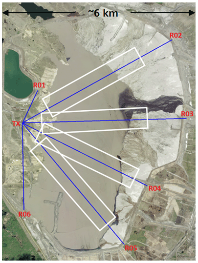
Figure 1 GreenLITE^™ system configuration at the tailings pond. Simulated area emission sources (white rectangles) used in the SCICHEM modeling scheme. (Image credit: CNRL, 2020).

The system that was deployed to the open-pit mine (57.328044^∘ N, 111.758565^∘ W) in 2019 for 6 weeks was configured to measure CH₄ with the ability to generate 2-D concentration and emission maps. For mapping capability, two GreenLITE^™ transceivers must be separated by a distance on the order of half the width of the area to be measured. In the deployed configuration at the mine, as shown in Fig. 2, the transceivers – denoted T1 and T2 – were located 960 m apart on the north edge of the mine pit. In total 15 reflectors, denoted R01 clockwise through R15, were installed along the east, south, and west edges of the mine. Chord lengths ranged from 440 m to 2.4 km. The cross-hatched measurement chord pattern, shown in Fig. 2, enabled the construction of 2-D maps of concentrations and emissions, based on a sparse tomography approach, that will be discussed later. Local surface weather data were used in the retrieval of gas concentration from optical depth and in the estimation of emissions from the mine. The objective of the 2019 measurement campaign at the mine was to estimate spatially resolved CH₄ emissions over an extended period.

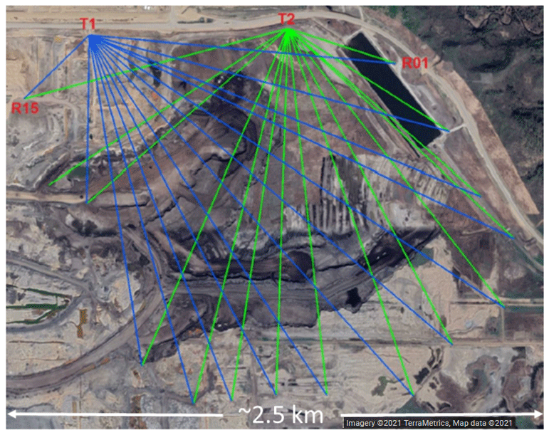
Figure 2 GreenLITE^™ system configuration at mine face.

In 2020, the GreenLITE^™ system was again installed at the tailings pond shown in Fig. 1, and in nearly the same configuration. The objective of the 2020 measurement campaign at the tailings pond was to observe and quantify any potential enhancement in emission during the time of pond ice thaw and breakup, as an emission outgassing during this time had been postulated (Small et al., 2015).

4 Emission estimation

The GreenLITE^™ concentration measurements were combined with locally measured surface weather information, including air temperature, humidity, air pressure, wind speed, and wind direction; publicly available numerical weather prediction (NWP) Rapid Refresh (Benjamin et al., 2016) upper-air model fields; and terrain information derived from the Canadian Digital Elevation Model (DEM) (NRCan (Natural Resources Canada), 2016) to form the inputs to the Second-Order Closure Integrated Puff Model with Chemistry (SCICHEM) dispersion model (Chowdhury et al., 2015) to estimate CH₄ emission rates. SCICHEM is based on the Second-Order Closure Integrated Puff (SCIPUFF) model (Sykes et al., 1986, Sykes and Gabruk, 1997), which was developed as a short-range dispersion model. A flow diagram depicting the emission estimation process is shown in Fig. 3. Measured concentrations for each measurement chord shown in Fig. 1 that passed over the pond, denoted by R02, R03, R04, and R05, were averaged on an hourly basis and background-corrected using the corresponding hourly-averaged concentration measurements from chords R01 and R06. Since R01 and R06 are most likely contaminated by pond emissions when winds have an easterly component, data were filtered for use in emissions estimates based on an acceptable wind range of 190 to 350^∘ to ensure that concentration measurements taken along chords R01 and R06 and used in background correction were upwind of the pond. The background chords formed by R01 and R06 were intentionally located on the west side of the pond since the prevailing winds for this site are out of the west.

Figure 3 Emission estimation flow diagram.

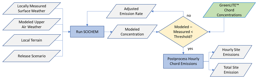
SCICHEM was run using continuous area source release scenarios as depicted by the notional white rectangles shown in Fig. 1. While the GreenLITE^™ concentration measurements that serve as input to the SCICHEM modeling framework are integrated measurements that span the pond and east beach, the SCICHEM model was limited to rectangular simulated release areas with constraints on release area dimensions. The simulated release area size depicted by the white rectangles shown in Fig. 1 were chosen to (1) cover the along-chord extent of pond that was assumed to be an emission source and (2) account for a SCICHEM (v3.2) bug that limited the simulated release area to be less than 360 m in one dimension. The simulated release areas for each chord measurement were centered at the midpoint of each respective chord. For any given set of chord measurements, SCICHEM was used to independently model the concentration in each rectangular box by computing a value given an initial guess at the associated emission rate. The initial guess is accounted for in the independent release scenario for each simulated release area. The differences between the hourly-averaged measured and modeled concentrations on a per-chord basis were then used in an iterative conjugate gradient scheme to adjust the emission rates until the modeled and measured concentrations matched within 0.0005 ppm. Once the values converged, the corresponding emission rates were recorded. Since the pond and east beach areas are considered as emission sources, the per-chord emission rates reported by SCICHEM (units of mass per unit time) were then normalized by the respective simulated release source areas of each chord to convert to flux (mass per unit time per unit area), averaged hourly for chords that transect the pond, and scaled by the estimated total pond (and east beach) area to provide hourly emission estimates for the entire site. This emission retrieval scheme was used to estimate CH₄ emission rates during both the 2019 and 2020 campaigns at the tailings pond for each hour that met the screening criteria for wind direction and included measurements that met a minimum signal-to-noise ratio (SNR) threshold.

A nearly identical approach was employed to estimate emissions from the open-pit mine in 2019. However, the simulated area release scenario used in the SCICHEM emission retrieval approach differed from that used at the tailings pond shown in Fig. 1 since the configuration at the mine (Fig. 2) allowed the development of 2-D maps of concentration at the approximate height of the plane formed by the measurement chords above the mine face. A plume-based model is used to predict the 2-D methane distribution associated with a collection of diffuse emission sources. An example of a plume-based 2-D concentration distribution estimate for the mine installation is shown on the left side of Fig. 4. The plume-based 2-D maps are used as the basis to formulate a reconstruction scheme with rectangular basis functions that were employed during the 2019 mine campaign to provide a direct interface to standardized emission model frameworks, such as SCICHEM. In the case of the mine, geo-referenced rectangles and local topography from historical DEMs are used to describe sub-sections of the mine and surrounding areas. An example of a box-based concentration reconstruction is shown on the right side of Fig. 4. The areal extent and concentration for each rectangle are directly integrated into the simulated release scenarios employed in the SCICHEM emission retrieval scheme. These boxes and rectangles serve the same purpose as the white rectangles shown in Fig. 1 for the pond. In the case of the mine, the CH₄ background concentration required by the dispersion modeling scheme was determined based on the box having the lowest concentration relative to all other boxes in a given 2-D distribution. A visual survey of 2-D box emission maps indicated that some portions of the mine were consistently emitting little or no CH₄, which supports the use of the lowest concentration box as an indication of background. However, an integrated-path measurement just upwind of the mine – as was done at the pond – would provide a more ideal estimate of immediate upwind background and will be explored in future applications. In this manner, emissions were estimated for all time periods that had a 2-D reconstruction, irrespective of wind direction, which was a constraint on the single-transceiver setup at the pond.

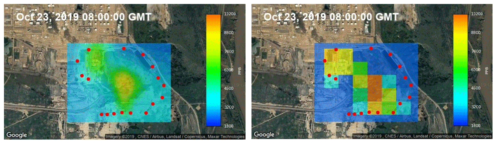
Figure 4 Example plume-based (left) and corresponding box-based (right) methane concentration reconstructions at the open-pit mine.

5 Results

5.1 Tailings pond emissions

CH₄ emission rates computed for the tailings pond are shown in Fig. 5 for both the summer 2019 and spring 2020 measurement campaigns. Gray data points represent hourly emission rates, and blue data points denote the two-day moving average. The negative hourly emission estimates seen in Fig. 5 are likely due to a combination of (1) measurement and emission estimate noise during periods of low pond emission when reported background concentration is higher than reported pond concentration and (2) periods of low pond emission when a natural gradient in CH₄ is present over the measurement site, which also results in higher measured background concentration versus pond concentration. Average daily emissions were 7.2 metric tons per day (t/d) during the July–October 2019 period and 5.1±2.9 t/d¹ during the March–July 2020 period. Accounting for the estimated area of the pond and east beach (17.7 km²), which is also treated as an emission source, these seasonal emission rates scale to annual fluxes of 1.48 and 1.05 t/ha/yr, respectively. Annual fluxes are reported here for the sake of qualitative comparison with other published studies. However, caution should be exercised when temporally extrapolating emission estimates since uncertainty may increase substantially given the temporal and seasonal variation in emissions. As can be seen in Fig. 5, emissions were higher and more variable in summer 2019 versus spring 2020. Several drivers may have contributed to this behavior. For example, the pond ice surface was frozen through a portion of the spring campaign, partially capping emissions from a large portion of the pond surface. The temporal variability in the results shown in Fig. 5 also indicates the potential for significant biases in annually reported emissions that are based on periodic measurements versus an extended or continuous measurement approach.

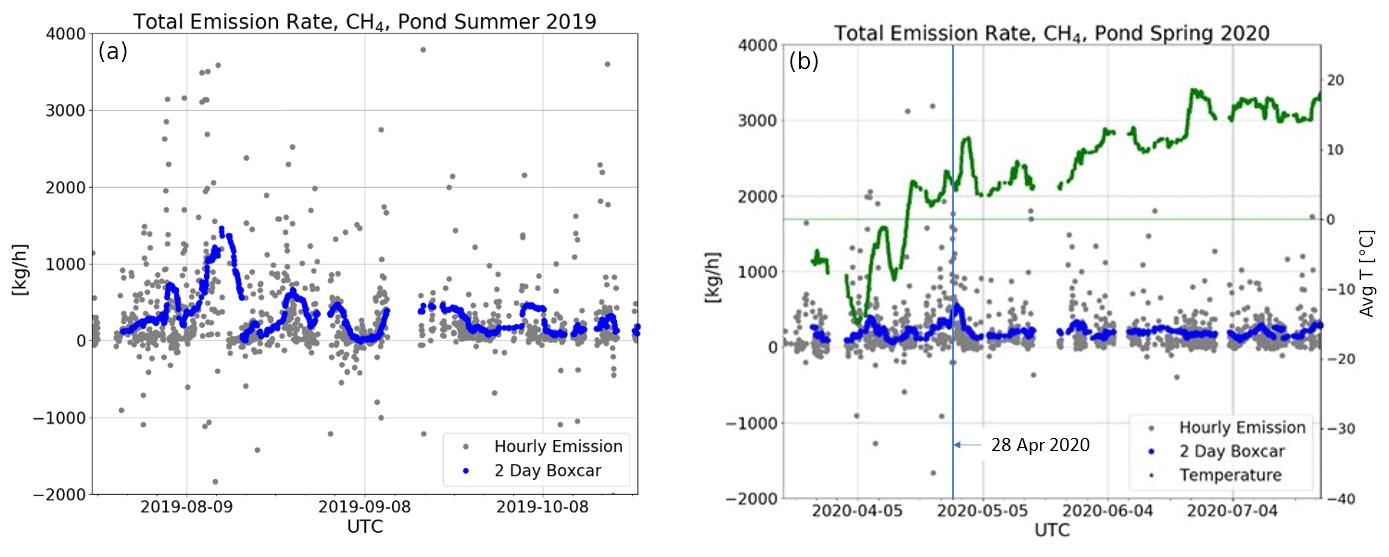
Figure 5 Tailings pond methane emissions for July–October 2019 (a) and March–July 2020 (b), including hourly emission (gray) and two-day moving average (blue). Two-day moving average of local air temperature (green) corresponds to the right most y axis.

As previously mentioned, a key motivation for the spring 2020 campaign was to measure and quantify any enhancement in emissions during the time period of pond ice breakup. First, to identify the period of pond ice breakup, local air temperature was studied as an indicator of ice thawing and eventual breakup. Daily high temperature was consistently above freezing beginning the second week of April, and daily average temperature was consistently above freezing beginning the third week of April (see Appendix A, Fig. A1). Furthermore, while the exact freezing and melting points of the tailings pond and nearby Athabasca River may vary due to differences in composition and dynamics, the local water level of the river was studied as an approximate indicator of regional ice thaw and breakup. The measured river water level through the last 2 weeks of April 2020 strongly implies river ice breakup during the last week of April (see Appendix A, Fig. A2).

Figure 5b shows CH₄ pond emission through the 2020 campaign along with the two-day moving average of local air temperature (green) for reference. Two emission enhancements are discernible that may be associated with ice breakup. The first occurs during the second week of April, which coincides with daily high air temperatures consistently above freezing. The second and higher magnitude enhancement occurs during the last week of April, which overlaps with daily average air temperature consistently above freezing and is close in time with the assumed ice breakup of the Athabasca River. The late-April enhancement peaked at 739 kg/h, based on the rolling two-day average, on 28 April 2020, and was 4 times the median hourly rolling average emission computed over the course of the 2020 campaign.

A diurnal pattern in CH₄ emission from the tailings pond was not discerned in an hour-of-day analysis of both summer 2019 and spring 2020 emission results, in contrast to Zhang et al. (2019), who reported 2.8 times higher CH₄ emission at night versus day based on EC measurements over a 13 d period at an Athabasca tailings pond in June 2012. However, a diurnal pattern was observed not only in measured CH₄ concentration over the pond, similar to that reported by Zhang et al. (2019), but also in the background concentration as seen in Fig. 6. The figure shows median hour-of-day concentration for the summer 2019 (a) and spring 2020 (b) measurement periods. The diurnal patterns seen in Fig. 6 are indicative of the daily planetary boundary cycle which compresses the near-earth atmosphere at night.

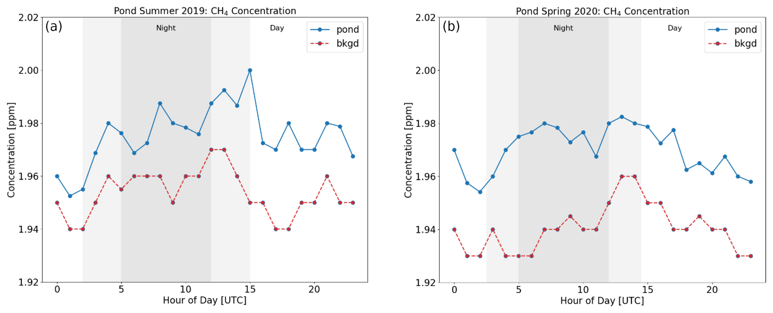
Figure 6 Tailings pond and background CH₄ median hour-of-day concentration for summer 2019 (a) and spring 2020 (b).

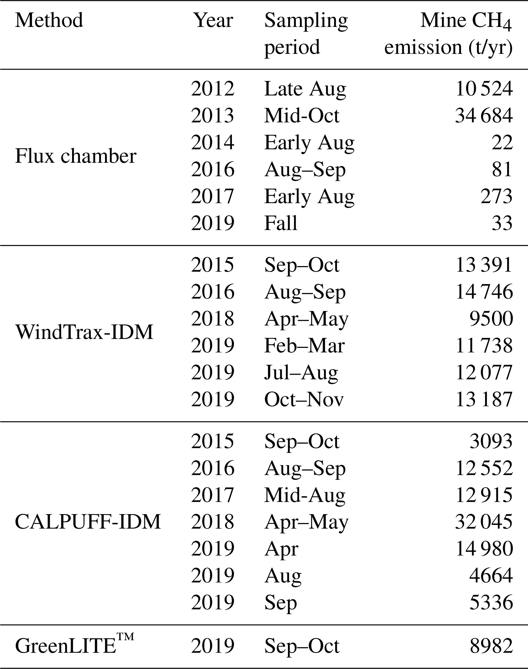
Several CH₄ emission studies have been conducted at the same tailings pond over the last decade. Results from many of these studies are summarized in Appendix A and Table A1 and plotted in Fig. 7 on a monthly basis. The measurement and emission estimation approaches covered include flux chamber, EC, and multiple point measurements with the WindTrax (http://www.thunderbeachscientific.com/, last access: 11 January 2022) IDM; multiple point measurements with the CALPUFF (http://www.src.com/, last access: 11 January 2022) IDM; and multiple open-path, integrated measurements with the SCICHEM IDM (GreenLITE^™). The emission values shown in Fig. 7 provide a qualitative comparison of several emission estimation techniques from multiple seasons over many years. As such, conclusions drawn from direct comparisons should be made with caution for several reasons, most of which have already been discussed. First, production at the site has increased over the past decade (CNRL Horizon 2010 oil sands production, 2022; CNRL 2019 end-of-year results, 2022; Canada's Energy Future 2017 Supplement, 2022), which, in theory, would result in larger quantities of tailings and higher CH₄ emissions over this time. Figure 7 shows a trend of increasing emission that may be indicative of the increase in production from the oil sands site, in addition to improved emission measurement techniques. Second, tailings pond CH₄ emissions have been shown to have a seasonal dependency. Lastly, the measurement footprint represented by each approach listed in Fig. 7 and Table A1 varies significantly, and tailings pond emissions are spatially heterogenous.

Figure 7 Historical tailings pond emission studies.

Figure 8 shows reported monthly bitumen production at the oil sands site during 2019 (a) and 2020 (b), with CH₄ tailings pond median monthly emission as computed with GreenLITE^™ overplotted. Since tailings produced will vary as a function of bitumen mined, so too will CH₄ pond emissions be expected to vary. As can be seen in the figure, CH₄ emissions trend well with bitumen production except for the first month of each respective GreenLITE^™ measurement campaign. Not coincidentally, both of the pond measurement campaigns began mid-month in July 2019 and March 2020, respectively, causing those months to be undersampled and further emphasizing the importance of continuous or longer-term measurement. Of 744 h in July, only 84 h were sampled near the end of the month during the summer 2019 campaign. Of 744 h in March, only 108 h were sampled near the end of the month during the spring 2020 campaign.

Figure 8 Bitumen production and GreenLITE^™ CH₄ tailings pond median monthly computed emissions (Alberta Energy Regulator, 2021).

5.2 Mine emissions

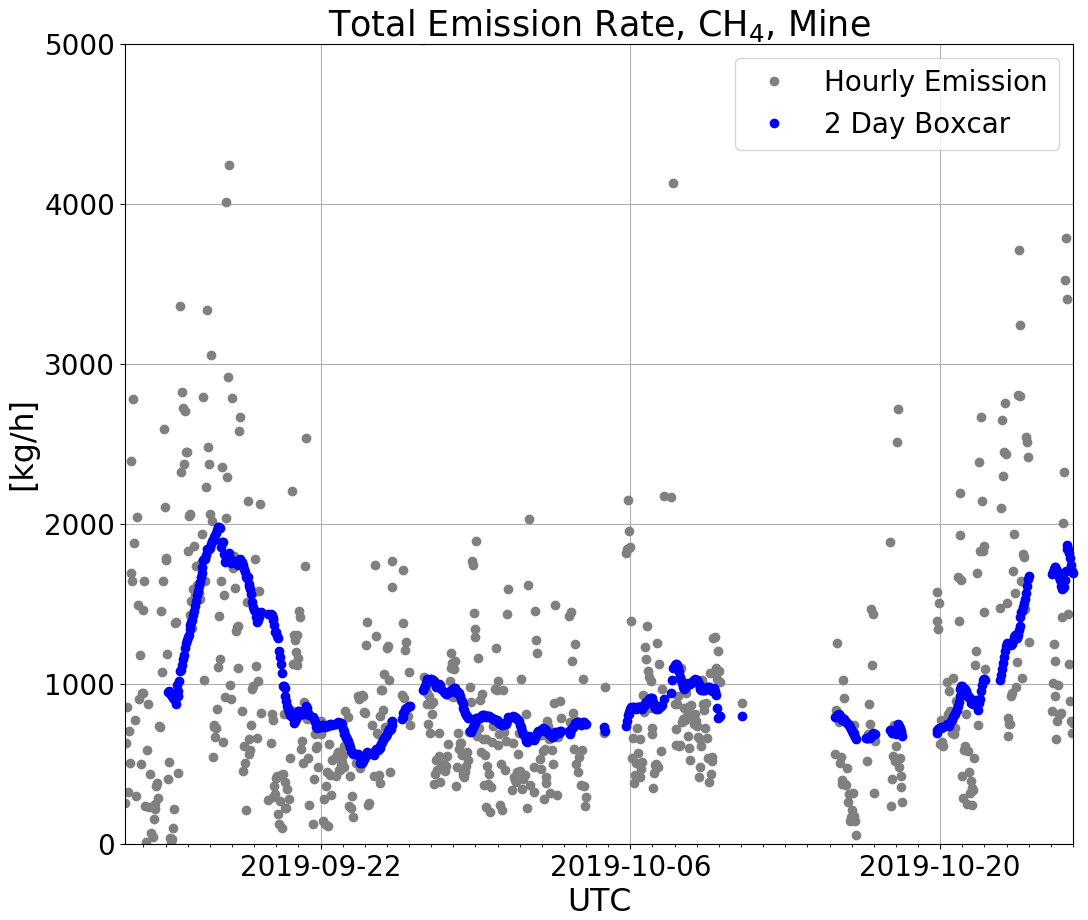
CH₄ emission rates computed for the mine are shown in Fig. 9. Gray data points represent hourly emission rates, and blue data points are the two-day moving average. In order to isolate emissions emanating from the face of the open-pit mine, known vented emission sources near the northeast boundary of the GreenLITE^™ measurement footprint were excluded from these analyses by simply not retrieving emission values for the 2-D concentration reconstruction boxes (as shown in Fig. 4, right) nearest to the known vented sources. Average daily emissions were 24.6 t/d during the approximately 6-week measurement period. Accounting for the estimated area of the mine pit at the time, measurements were taken (3.8 km²), and the average daily emission rate scales to an annual flux of 24.5 t/ha/yr. Similar to the temporal variations seen in tailings pond emissions, the variability in estimated mine emissions shown in Fig. 9 are modulated by mine activity, the associated localized wind pattern, and atmospheric state. The variability over this 6-week period again emphasizes the potential for significant biases in annually reported emissions that are based on short periodic measurements versus a continuous or long-term measurement approach.

Figure 9 Open-pit mine methane emissions.

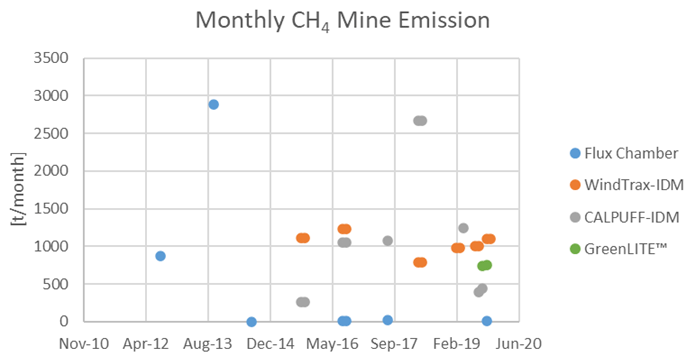
Like the tailings pond, several CH₄ emission studies have been conducted at local mine pits over the last decade using many of the same measurement and emission estimation techniques. Results from these studies are summarized in Appendix A and Table A2 and plotted in Fig. 10 on a monthly basis. Once again, the emission values shown in Fig. 10 provide only a qualitative comparison of emission estimation techniques from multiple seasons and years due to the utilization of measurement footprints that vary significantly.

Figure 10 Historical mine emission studies.

5.3 Uncertainty and error in estimates of emissions

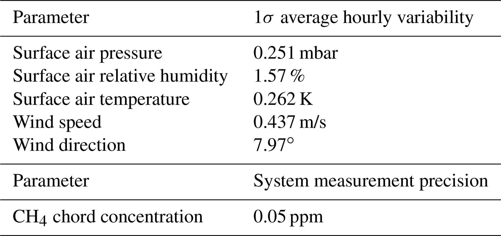
Several factors contribute to uncertainty in estimates of emissions from both the pond and mine environments. Such factors include the accuracy of measured surface meteorology, measured concentrations, and IDM fidelity and user-defined parameters, such as source emitter size and location and input terrain information. Preliminary Monte Carlo-style simulations were run to quantify the error in retrieved emission rates associated with variability in surface meteorology and instrument measurement precision. Hourly estimates of emissions are achieved by averaging the primary dispersion model input parameters on an hourly basis – namely, measured chord gas concentration, surface air temperature (T), surface air pressure (P), surface air relative humidity (RH), wind direction, and wind speed. Hourly variability in surface air T, P, and RH; wind speed; and wind direction were quantified by averaging hourly variability over three separate days during the GreenLITE^™ pond measurement campaign in spring of 2020. Of the many days for which wind consistently had a westerly component, which allowed for emissions to be computed for all or most hours of the day, the three days chosen at random were 22 and 27 March and 8 April 2020, and the resulting variances are shown in the top portion of Table 1. Previously determined GreenLITE^™ instrument measurement precision was used for variability in measured chord concentrations and is provided at the bottom of Table 1. Emissions were retrieved for a given day and hour over 10 runs while varying input quantities by uniform random distribution that spanned $+/-$ the average hourly variability (surface meteorology) and instrument measurement precision in Table 1. The variance in resulting emissions over the 10 runs represents the error associated with variability of surface meteorology and instrument precision in retrieved hourly emission values, as shown in Table 2. The results shown in Table 2 indicate that either weather and concentration measurement accuracy, actual weather and concentration variability over the 1 h averaging interval, or both are significant contributors to retrieved emission uncertainty. Future work may explore averaging windows greater and less than 1 h to assess the resulting impact on emission retrieval uncertainty. Furthermore, this Monte Carlo style of error quantification will be formalized and run independently for each future measurement campaign, or perhaps on a continuous weekly or monthly basis during a given measurement campaign.

Table 1 Meteorological parameter variances and system measurement precision used in Monte Carlo simulation.

Table 2 Emissions error results of Monte Carlo simulation.

Dispersion models have intrinsic uncertainties of their own. Chowdhury et al. (2015) carried out an inert tracer study to characterize the performance of SCICHEM in predicting plume dispersion. In the study, SCICHEM results were compared to plume measurements taken downwind of the tracer release point. At 2 km downwind, Chowdhury et al. (2015) reported a normalized mean square error (NMSE) of 2.18 % and a normalized mean bias (NMB) of 0.63 % in observed versus predicted plume concentration. Based on the estimated emission sensitivity to uncertainty in concentration that was characterized in the aforementioned Monte Carlo studies, the errors reported by Chowdhury correspond to errors in estimated emissions of $\mathrm{5.8}\times {\mathrm{10}}^{-\mathrm{6}}$ and $\mathrm{1.3}\times {\mathrm{10}}^{-\mathrm{6}}$ t/d, respectively. The Chowdhury study was conducted under topographical conditions that are assumed to be well defined. Another key difference worth noting between the Chowdhury study and the GreenLITE^™ oil sands application is the use of a tracer point source versus modeled extended source. The reported IDM errors associated with modeling a point source can be expected to scale upward for an extended source. Future work will include characterization of IDM uncertainty as used with GreenLITE^™ measurements in the oil sands environment.

Global semi-static DEMs are ill-suited to describe the dynamic landscapes of tailings ponds and open-pit mines. The areas of the tailings pond and mine that are considered as sources of emissions comprise a fraction of the total area of terrain passed into and taken into account by SCICHEM – 8 % for the pond and 11 % for the mine. Still, approximated terrain for the tailings pond and especially the open-pit mine for which SCICHEM simulations were performed may impact the accuracy of dispersion modeling and subsequent emission estimates. Irrespective of the measurement approach used with an IDM, IDMs, like any atmospheric model or emission estimation approach, are inherently less accurate in complex topographies and environments where horizontal homogeneous meteorology cannot be assumed (Flesch et al., 2005; Hu et al., 2016), and in particular for a relatively large depression such as an open-pit mine (Nahian et al., 2020). Future work should utilize current topography in dispersion modeling whenever possible to minimize these errors. In future work we may also explore a Monte Carlo simulation where measurement height relative to simulated release point (representing mine depth) is varied to assess the impact on retrieved emissions. Recent work in computational fluid dynamic modeling (Kia et al., 2021) has attempted to characterize meteorological fields associated with open-pit mines. Results of such work could potentially be incorporated into emission retrievals that are based on IDM to reduce error due to complex terrain but may be computationally prohibitive for a near-real-time emission monitoring application.

As discussed in Sect. 4, the simulated release area size depicted by the white rectangles shown in Fig. 1 were chosen to (1) cover the along-chord extent of pond that was assumed to be an emission source and (2) account for a SCICHEM (v3.2) bug that limited the simulated release area to be less than 360 m in one dimension. An idealized simulation would consider the entire pond and west beach as emission sources. For this reason, a study was performed to characterize the relationship between simulated release area size and retrieved emissions. As may be expected, it was found that larger release areas in the cross-wind direction produced larger emission estimates, while larger release areas in the along-wind direction produced smaller emission estimates. Future work should utilize a later version of SCICHEM that allows for release areas to be greater than 360 m in all dimensions, or an alternate IDM, to allow for flexibility in determining and implementing ideal release area sizes, shapes, and locations which will improve the accuracy in estimated emissions.

6 Conclusions

A novel approach to estimate fugitive emissions from the mine pit and tailings pond of a large oil sands operation has been demonstrated that utilizes the GreenLITE^™ gas measurement system and the SCICHEM IDM. CH₄ emissions from a tailings pond were estimated to be 7.2 t/d for July–October 2019, and 5.1±2.9 t/d for March–July 2020. CH₄ emissions from the mine pit were estimated to be 24.6 t/d for September–October 2019. Estimated emission rates for both the tailings pond and mine are in family with several recent studies at the oil sands site that employed a variety of measurement and emission estimation approaches. Emissions from wide area sources, such as oil sands tailings pond and open-pit mines, tend to vary both spatially and temporally. For the purposes of (1) emission regulation reporting and compliance and (2) emission mitigation planning, implementation, and assessment, an ideal measurement solution would include continuous measurement over extended time periods and cover an area of interest with spatial resolution high enough to identify and apportion emissions to specific sectors within the measurement footprint. The continuous, integrated-path, wide-area coverage of the GreenLITE^™ system was used to estimate and apportion CH₄ emission at the open-pit mine as implemented in the two-transceiver configuration, which allows for 2-D mapping. While 2-D mapping is not possible in the one-transceiver configuration employed at the tailings pond, apportionment of emissions is possible to a lesser degree and improves with the number of measurement chords passing over the assumed emission source.

The approach demonstrated here may be applicable to a variety of wide-area emission scenarios, to include oil and gas production, wastewater treatment plants, landfills, feedlots, wetlands, permafrost, cities, and shipping ports. Future work may involve comparisons of emissions results using additional, alternative IDMs, and should incorporate current topography in dispersion modeling whenever possible. Future work will also include a continuous approach to error estimation for each measurement application. Furthermore, a flux-gradient approach may be explored in a future GreenLITE^™ deployment utilizing concentration measurements at multiple heights. Such an approach could reduce the computational expense associated with the IDM method.

Appendix A: Supporting data

Figure A1 shows daily high, average, and low air temperature as measured at the pond site during early spring of 2020.

Table A1 Historical tailings pond emission studies (AECOM Canada Ltd., 2021).

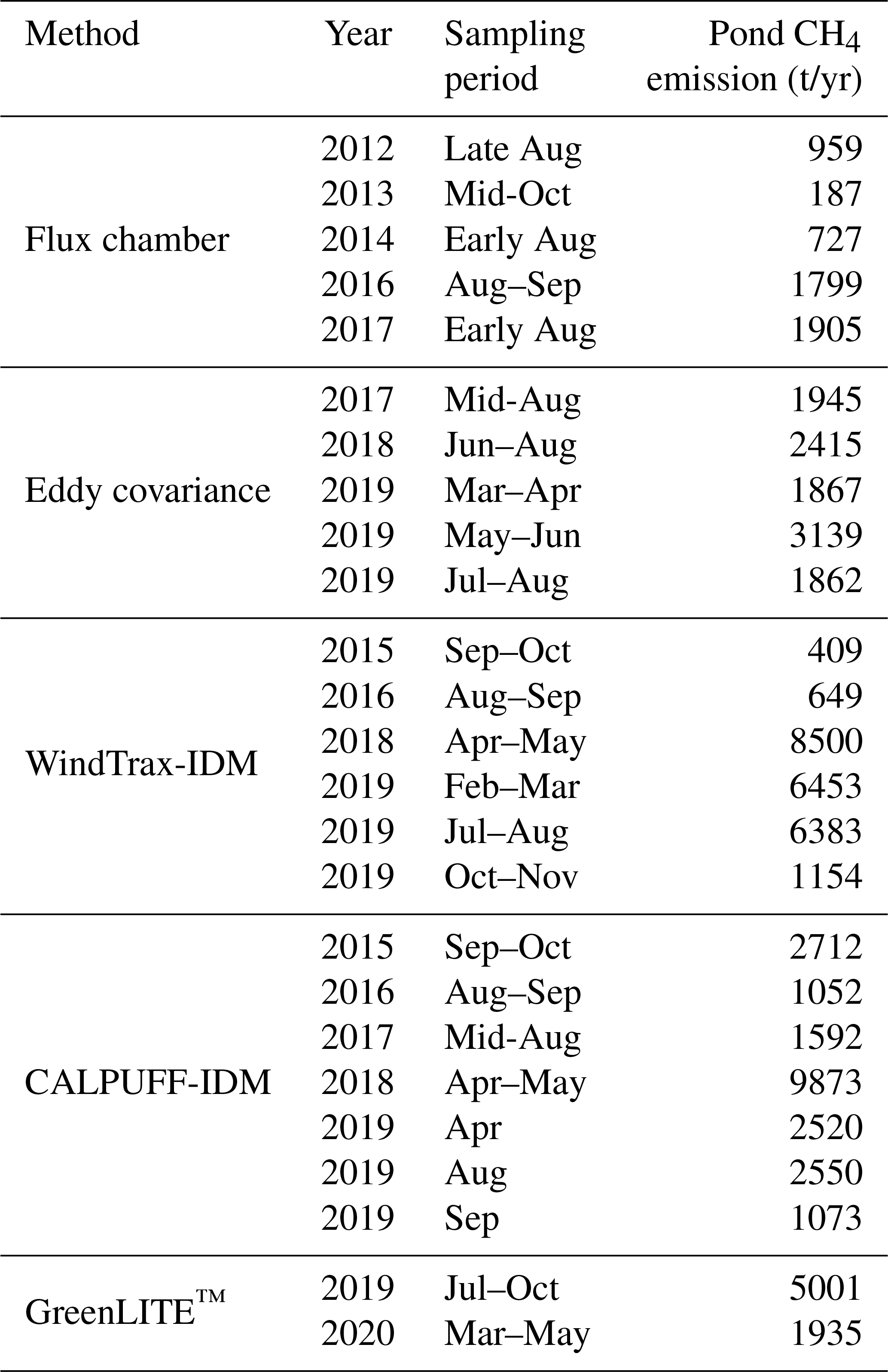
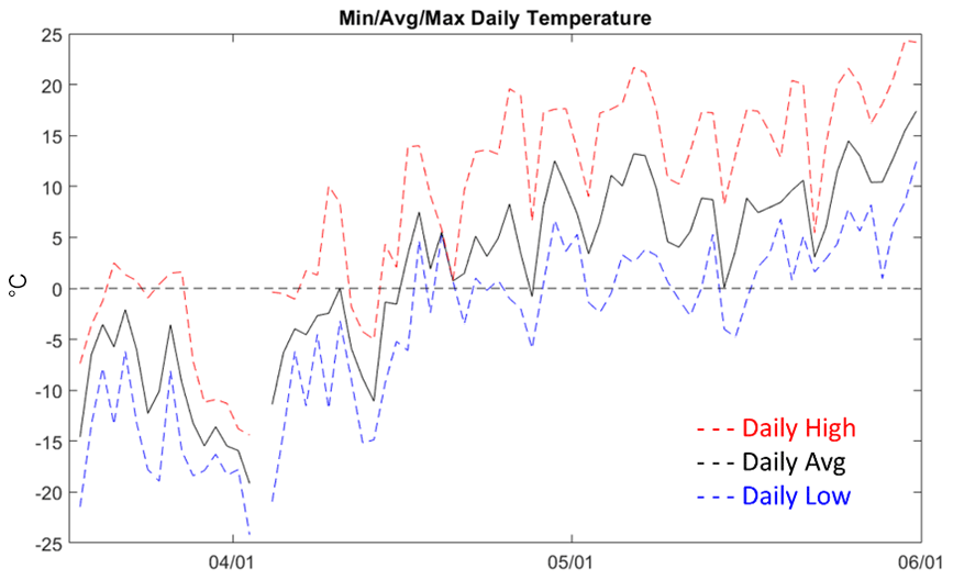
Figure A1 Daily high, average, and low air temperature at tailings pond site during spring 2020.

Figure A2 shows the measured river water level through the last 2 weeks of April 2020.

Figure A2 Athabasca River water level (Government of Canada, 2021).

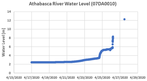
Table A1 shows a summary of CH₄ emission studies performed at the tailings pond over the last decade.

Table A2 shows a summary of CH₄ emission studies performed at the mine over the last decade.

Table A2 Historical open-pit mine emission studies (AECOM Canada Ltd., 2021).