the Creative Commons Attribution 4.0 License.
the Creative Commons Attribution 4.0 License.
 | 11 May 2022
Airborne measurements of directional reflectivity over the Arctic marginal sea ice zone
Sebastian Becker
André Ehrlich
Evelyn Jäkel
Tim Carlsen
Michael Schäfer
Manfred Wendisch
The directional reflection of solar radiation by the Arctic Ocean is mainly shaped by two dominating surface types: sea ice (often snow-covered) and open ocean (ice-free). In the transitional zone between them, the marginal sea ice zone (MIZ), the surface reflection properties are determined by a mixture of the reflectance of both surface types. Retrieval methods applied over the MIZ need to take into account the mixed directional reflectivity; otherwise uncertainties in the retrieved atmospheric parameters over the MIZ may occur. To quantify these uncertainties, respective measurements of reflection properties of the MIZ are needed. Therefore, in this case study, an averaged hemispherical–directional reflectance factor (HDRF) of the inhomogeneous surface (mixture of sea ice and open ocean) in the MIZ is derived using airborne measurements collected with a digital fish-eye camera during a 20 min low-level flight leg in cloud-free conditions. For this purpose, a sea ice mask was developed to separate the reflectivity measurements from sea ice and open ocean and to derive separate HDRFs of the individual surface types. The respective results were compared with simulations and independent measurements available from the literature. It is shown that the open-ocean HDRF in the MIZ differs from homogeneous ocean surfaces due to wave attenuation. Using individual HDRFs of both surface types and the sea ice fraction, the mixed HDRF describing the directional reflectivity of the inhomogeneous surface of the MIZ was retrieved by a linear weighting procedure. Accounting for the wave attenuation, good agreement between the average measured HDRF and the constructed HDRF of the MIZ was found for the presented case study.
- Article
(7383 KB) - Full-text XML
- BibTeX
- EndNote


The Arctic Ocean is a key component of the complex Arctic climate system. From a solar radiative point of view, the surface of the Arctic Ocean is characterized by the strong contrast between the highly reflecting sea ice and the rather absorbing open ocean, which both determine the surface solar radiative energy budget. The reflection properties of both surface types are strongly linked to the sea ice–albedo feedback, which significantly contributes to Arctic amplification (Pithan and Mauritsen, 2014; Wendisch et al., 2017). Often, the sea ice is covered by snow. The spectral albedo of the snow-covered Arctic sea ice typically varies between 0.8 and 0.9 in the visible spectral range (Wiscombe, 1980), depending on the snow cover, grain size, melt pond fraction, and solar zenith angle (SZA). In contrast, solar radiation is mostly absorbed by open ocean. Its albedo depends on the surface wind speed and SZA and typically ranges below 0.1 for SZAs smaller than 65∘ in clear-sky conditions (Jin et al., 2004; Feng et al., 2016).
The reflection of solar radiation by snow-covered sea ice and open-ocean surfaces was extensively studied and characterized by ground-based, airborne, and satellite observations (e.g., Cox and Munk, 1954; Gatebe et al., 2003; Bourgeois et al., 2006). However, large areas of the Arctic Ocean are characterized by a mixture of sea ice and open ocean. The open water might be formed by leads or polynyas, while sea ice may also be covered by melt ponds (e.g., Hoffman et al., 2019). Also, in the marginal sea ice zone (MIZ), individual ice floes of different size cover varying fractions of the ocean. Strong and Rigor (2013) defined the MIZ as the zone where the sea ice concentration ranges between 0.15 and 0.8. In a warmer Arctic, the sea ice cover will further decrease (Perovich et al., 2018) and first-year sea ice will become more dominant. Accordingly, a significant reduction in the sea ice thickness has been observed (Kwok, 2018). In summer, the thinner sea ice is more dynamic and breaks more easily, which leads to a higher number of leads, a stronger drift, a faster dispersion of the floes, and a more extended MIZ (Kashiwase et al., 2017). Strong and Rigor (2013) showed that the width of the MIZ increased by about 13 km per decade in summer, resulting in a widening of 39 % between 1979 and 2011. Accordingly, the summertime MIZ nowadays covers between 20 % and 60 % of the entire Arctic sea ice extent (Rolph et al., 2020). In winter, when the MIZ is dominated by freshly frozen sea ice, no significant trend of the MIZ extent was observed. The summertime MIZ-widening trend highlights the necessity for characterizing the radiative properties of the mixture of sea ice and open ocean, which is needed to better quantify the complex radiative processes in such areas.
To quantify the solar radiative energy budget at the surface, the surface albedo as a hemispherically integrated measure of reflection is sufficient (e.g., Stapf et al., 2020). However, satellites detect the directional reflection instead of the surface albedo, such that conversion methods quantifying the surface reflection characteristics of all directions need to be applied (e.g., Schaaf et al., 2002). The directional distribution of the reflected radiances (as a fraction of the incident radiation) is often quantified by the bidirectional reflectance distribution function (BRDF, mostly used in models) or the directly measurable hemispherical–directional reflectance factor (HDRF; Nicodemus et al., 1977; Schaepman-Strub et al., 2006). While the BRDF only considers direct illumination from one single direction, diffuse illumination from the entire hemisphere is also taken into account by the HDRF.
The HDRF of homogeneous snow/sea ice and open-ocean surfaces has been derived from measurements and simulations in numerous studies (e.g., Bourgeois et al., 2006; Gatebe et al., 2003). The HDRF of snow is characterized by high reflectance, which is further enhanced in the forward direction (i.e., at high reflection zenith angles around 0∘ relative azimuth). This forward peak increases relative to the reflectance in the nadir direction with an increasing solar zenith angle and wavelength (e.g., Warren et al., 1998; Aoki et al., 2000; Carlsen et al., 2020). Similarly to the albedo, the snow HDRF depends on snow morphology (i.e., snow grain size and shape), which is crucial for accurate simulations of the snow HDRF (Jafariserajehlou et al., 2021). Despite the low reflectance of open ocean for most reflection directions, in the so-called sunglint angular range, specular reflection can be several orders of magnitude higher. The width and maximum intensity of the sunglint area depend on surface roughness and, thus, on the wind speed. The higher the wind speed, the rougher the surface and the broader the sunglint area but the lower its maximum intensity (e.g., Cox and Munk, 1954; Jackson and Alpers, 2010).
Quantitative measurements of the HDRF of snow and open ocean have been obtained by ground-based, airborne, and satellites observations. Bourgeois et al. (2006) and Marks et al. (2015) retrieved the HDRF of snow using a ground-based goniospectrometer, which measures the spectral radiance reflected from a small surface area from different directions. Their measurements provide an angular resolution of about 15∘ with a spectral resolution in the range of 1 nm. Commercial digital cameras equipped with a 180∘ fish-eye lens deliver instantaneous radiance observations as a function of reflection directions of the lower hemisphere with high angular resolution (<0.5∘). In both cases, the downward spectral irradiance measured by a spectral hemispherical radiometer is required for the derivation of the HDRF. Goyens et al. (2018) combined ground-based goniospectrometer and fish-eye camera observations to benefit from both the hyperspectral and the hyperangular resolution. Since goniospectrometers are restricted to observations over solid ground, mostly shipborne or airborne measurements are used to derive the HDRF of open ocean (Cox and Munk, 1954). Gatebe et al. (2005) retrieved the open-ocean wind speed and BRDF using the Cloud Absorption Radiometer (CAR), which is a scanning radiometer with a field of view (FOV) of 190∘. This wide FOV is achieved by scanning the lower hemisphere with a narrow FOV optic of about 1∘ using a scanning mirror.
Airborne observations using a digital camera equipped with a wide-angle lens have been reported by Ehrlich et al. (2012). Although the spectral resolution of the camera is limited to the three visible channels of red, green, and blue (RGB), this technique was applied to analyze the impact of surface winds on the HDRF of the ocean surface. For homogeneous snow-covered areas in the Antarctic, Carlsen et al. (2020) used airborne 180∘ fish-eye camera observations to quantify the anisotropy of the snow HDRF with changing surface roughness, snow grain size, and SZAs.
Most of the previous ground-based and airborne BRDF studies have focused on specific homogeneous surface types. The reflectivity of an inhomogeneous surface, such as the MIZ, has rarely been observed. Qu et al. (2016) combined simulated BRDFs of different surface types in the MIZ in order to retrieve the surface albedo of the MIZ from satellite observations. However, ocean waves are attenuated (Kohout et al., 2011) and the dependence of the sunglint on the surface roughness and the wind speed could differ from ice-free open oceans.
In this study, the hemispherical coverage and high spatial resolution of airborne fish-eye camera observations are used to characterize the HDRF of a mixture of open-ocean and partly snow-covered sea ice surfaces in the MIZ. After the introduction of the quantities used, as well as the observations and instruments, in Sect. 2, the following two questions will be discussed: (i) how does the HDRF of the individual contributions of open ocean and sea ice in the MIZ differ from homogeneous surfaces? To answer this, the contributions of the individual surface types on the observed mixed scenes are separated applying a sea ice mask (Sect. 3) and compared to HDRFs of homogeneous surfaces (Sect. 4). (ii) Is it possible to combine the HDRF of the individual surfaces, weighted by the sea ice fraction, to obtain a representative MIZ HDRF? For this, the data set is divided into two subsets. The previously separated HDRFs of one subset are recombined and compared to the (unseparated) mean of the other subset (Sect. 5).
2.1 Definition of reflectance quantities
The spectral BRDF fBRDF of a surface describes the directional distribution of the reflected radiation and is defined as
(Nicodemus et al., 1977). Fi represents the spectral irradiance (in ) illuminating (subscript “i”) a surface at wavelength λ from the direction characterized by the incident zenith and azimuth angles, θi and ϕi, respectively. Ir quantifies the radiance (in ) reflected (subscript “r”) in the direction characterized by the reflection zenith and azimuth angles, θr and ϕr, respectively, and depends additionally on the incident angles. The BRDF has the unit of inverse steradians (sr−1). Often the bidirectional reflectance factor (BRF) RBRF is used instead of the BRDF. The reflectance factor (dimensionless) is defined as the ratio of the BRDF of the actual surface to the constant BRDF of a Lambertian surface fBRDF,id, which is constantly equal to sr−1. Thus
Since the illumination under atmospheric conditions is a combination of a direct and a hemispherical diffuse irradiance component with the fractions fdir and , respectively, both BRDF and BRF cannot be measured practically. Therefore, the hemispherical–directional reflectance factor (HDRF, dimensionless) RHDRF is introduced (e.g., Schaepman-Strub et al., 2006):
The reflectance factor of the diffuse radiation incident over the entire hemisphere is denoted by , where 2π refers to the diffuse radiation incidence. The direction of the direct component is given by θi and ϕi. The spectral dependence is omitted here. If the diffuse fraction of the incident radiation is sufficiently small, the HDRF represents a good approximation of the BRF. The infinitesimal quantities in Eqs. (1)–(3) are not measurable; in practice, measurement optics with sufficiently small opening angles are applied to approximate the finite radiances. Thus, from a measurement perspective, the HDRF is obtained by
2.2 Observations and instrumentation
2.2.1 Airborne campaign
In this paper, data collected during the Arctic CLoud Observations Using airborne measurements during polar Day (ACLOUD; Wendisch et al., 2019) campaign, which took place in May and June 2017, are analyzed. During ACLOUD, the MIZ was located at about 80∘ N in the region northwest of Svalbard. A total of 19 measurement flights were conducted with each of the two research aircraft Polar 5 and Polar 6 from the Alfred Wegener Institute, Helmholtz Centre for Polar and Marine Research (AWI; Wesche et al., 2016). Both aircraft were equipped with downward-looking 180∘ fish-eye cameras measuring the upward directional radiances (Ehrlich et al., 2019; Jäkel et al., 2019b). Additionally, on Polar 5 the Spectral Modular Airborne Radiation measurement sysTem (SMART; Wendisch et al., 2001) was operated to measure the spectral downward solar irradiance.
The data analyzed for the present case study were obtained during the flight on 25 June 2017 (flight number 23) performed under cloudless conditions. Figure 1a shows a satellite image from the Moderate Resolution Imaging Spectroradiometer (MODIS) instrument on board the satellite Terra during the research flight. The surface was dominated by an inhomogeneous distribution of sea ice floes with diameters of up to several kilometers. The flight track of Polar 5 is plotted in red in Fig. 1a. A 20 min leg performed between 12:26:35 and 12:46:47 UTC (highlighted in yellow in Fig. 1a) was selected for the analysis, which ensures stable environmental conditions. The solar zenith angle ranged between 57.7 and 58.0∘ with a mean of 57.8∘. The observations were conducted along a 30 km straight flight section, during which the flight altitude varied between 65 and 165 m.
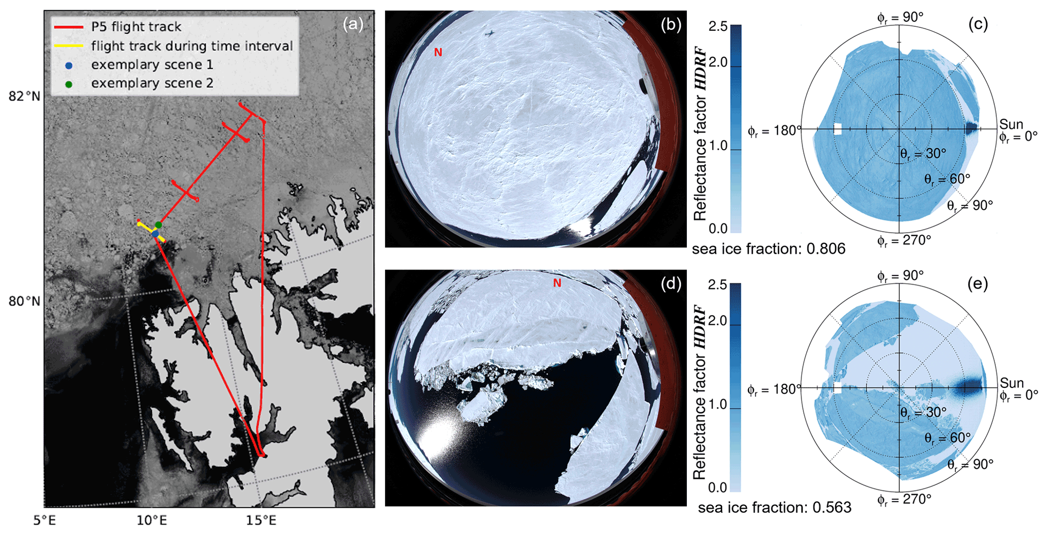
Figure 1(a) Satellite image (composed of MODIS bands 1 and 2) of the MIZ north of Svalbard observed on 25 June 2017, 12:45 UTC, including the flight track of Polar 5 (red). The 20 min period used for the analysis is highlighted in yellow. The blue and green dots indicate the locations where the exemplary scenes in (b) and (d), respectively, were observed. Panels (b) and (d) show exemplary images taken by the fish-eye camera at 12:37:23 and 12:46:41 UTC, respectively. Panels (c) and (e) present the processed HDRF polar plots of the scenes shown in (b) and (d), respectively. Note that the polar plots are rotated compared to the raw images in a manner that the solar incident direction is always to the right of the plot.
2.2.2 180∘ fish-eye camera
The upward radiance was measured by a Canon EOS-1D Mark III digital camera equipped with a 180∘ fish-eye lens. Images with a resolution of 3906×2600 pixels were taken every 6 s. As is common for commercial cameras, each pixel covers three spectral channels (RGB) centered at wavelengths of 591 (red), 530 (green), and 446 nm (blue) with a full width at half maximum (FWHM) of about 80 nm (Ehrlich et al., 2019; Carlsen et al., 2020). Figure 1b and d show two examples of raw true-color images taken by the fish-eye camera. The camera was calibrated in terms of geometrical, spectral, and radiometric characteristics, which allows a conversion of the measured raw data into radiances as described in detail by Carlsen et al. (2020). In contrast to Carlsen et al. (2020), who applied a stellar method for the geometrical calibration, images of checkerboards taken from different perspectives served as reference in this study. The images were analyzed by the open-source routine Cv2.FishEye from the free programming library OpenCV (http://opencv.org, last access: 18 August 2020; Jiang, 2017). The backward model described by Urquhart et al. (2016) was applied to calculate the camera-fixed viewing zenith and azimuth angles, θv and ϕv, respectively, of each image pixel using the OpenCV output parameters.
The fish-eye camera was fixed to the aircraft frame. To obtain radiance measurements with respect to an Earth-fixed coordinate system, the viewing angles (θv, ϕv) of each camera pixel were corrected to consider the aircraft attitude angles (roll, pitch, yaw). Euler rotation matrices were applied to transform the viewing angles into the reflection angles (θr and ϕr) (Ehrlich et al., 2012). The azimuth plane of the images was rotated with respect to the relative position of the Sun, such that the Sun (and the forward direction) is located at the right in all polar plots shown in this paper. The footprint of one single image varied between 380 and 915 m for the altitude range of the 20 min leg, assuming that the effective FOV of the fish-eye lens is 160∘.
2.2.3 Calculation of and uncertainty in the HDRF
Combining the downward irradiance Fi measured by SMART (Jäkel et al., 2019a) and the angularly resolved radiances Ir from the fish-eye camera (Jäkel and Ehrlich, 2019) allows the calculation of the HDRF at flight altitude (Eq. 4), whereby the spectrally resolved irradiances were converted into the spectral range of each camera channel using the individual relative spectral response function from the spectral calibration.
The uncertainty in the radiometric calibration of the fish-eye camera was estimated at 4 %; further uncertainties stem from the sensor characteristics and the combination of geometric calibration and aircraft attitude correction (0.5 % and 1 %, respectively; Carlsen et al., 2020), leading to a total uncertainty in the fish-eye camera radiance measurements of about 4.2 %. However, during ACLOUD, complementary radiance measurements were performed with SMART and a spectral imager, which demonstrated deviations of up to 35 % for the blue channel, while reflected radiances measured in the green and red channels ranged within the measurement uncertainties (Ehrlich et al., 2019). As a consequence, the fish-eye camera was inter-calibrated with SMART. The radiances measured in the red channel showed the best agreement in the instrument intercomparison (root mean square deviation of 0.01 and correlation coefficient of 0.98 between SMART and camera radiances; Ehrlich et al., 2019). The choice of the channel has only minor impact on the results presented here. While the reflectance of snow is spectrally neutral in the visible range, the spectral open-ocean albedo is only slightly higher in the blue than in the red channel. Therefore, it was decided to use the red camera channel in the following.
According to Bierwirth et al. (2009), the total uncertainty in the SMART irradiance measurements is 3.2 % in the visible spectral range. However, an updated transfer calibration (3 % error) and a larger cosine correction error (2 %) due to the larger solar zenith angle lead to an increased total uncertainty of 4.3 %. Thus, using the Gaussian error propagation, the total uncertainty in the calculated HDRF amounts to about 6 %.
Radiative transfer simulations performed with the library for radiative transfer (libRadtran; Mayer and Kylling, 2005; Emde et al., 2016) were used to estimate the impact of the atmosphere between the ground and the maximum flight altitude (165 m) on the measured HDRF. They have shown that the difference between the HDRF at ground and flight level is less than 1 % for the red camera channel.
The fully calibrated and processed HDRFs obtained from the exemplary raw images in Fig. 1b and d are shown in Fig. 1c and e, respectively. The region contaminated by the shadow of the aircraft (; ) was excluded and is represented by the white gap in the polar plots. The HDRF plots of the exemplary scenes reveal a high contrast between sea ice and open-ocean areas and show a largely enhanced HDRF in the sunglint region of open ocean.
3.1 Sea ice mask
The set of images of a low-level flight section of 20 min was filtered for larger turns with roll or pitch angles larger than 5∘. The remaining 138 fish-eye camera images were analyzed. Most of the individual images show a mixture of sea ice and open ocean. To obtain separate HDRFs for either surface type, a sea ice mask is constructed that considers the different reflection characteristics of both surface types. Figure 2 (black line) shows a frequency distribution of all HDRF measurements, merging all images and all directions (pixels). The histogram reveals a distinct separation of the data into two modes, originating from open ocean and sea ice. Accordingly, all pixels with HDRF values below a threshold of h1=0.3 are assigned to open ocean and pixels with HDRF values above a second threshold of h2=0.6 are mostly related to sea ice but can also be assigned to open ocean in the case of specular reflection observations. HDRF values between both thresholds, which are mostly linked to the ice floe edges, amount to roughly 3 % of the data and were excluded from further analysis.
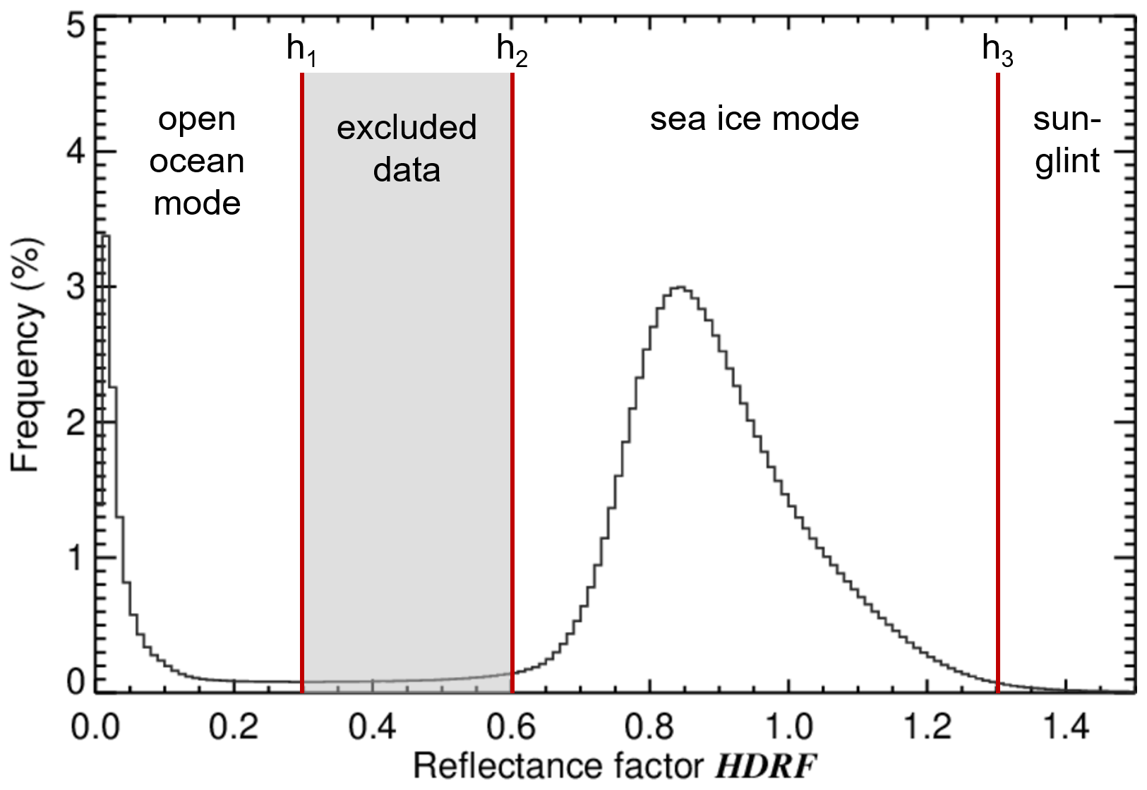
Figure 2Frequency distribution of the observed HDRF for all directions and all images. The three vertical red lines indicate the thresholds of h1=0.3, h2=0.6, and h3=1.3 applied in the sea ice mask algorithm.
In the sunglint region, the HDRF of open ocean can also feature values similar to or even exceeding typical values of sea ice. This sunglint area was identified by two additional criteria. Firstly, HDRF values larger than a third threshold of h3=1.3 were considered sunglint and assigned to open ocean. Secondly, a color ratio defined by the ratio of the radiances measured in the red (Ired) and the blue (Iblue) camera channel was used to identify the edges of the sunglint zone. Since the sunglint area appears more yellowish than the sea ice, its color ratio is higher. A color ratio threshold of was chosen for the separation of sea ice and sunglint when the HDRF was between h2 and h3. In Fig. 3a the color ratio of the exemplary scene (same as in Fig. 1d) is shown with values higher than 0.95 highlighted in red. Figure 3b illustrates the surface types identified by the sea ice mask. Together, both panels show the capability of this simple approach to separate between the surface types. Misclassifications mainly affect pixels at the sunglint margin (misclassified as sea ice), which do not have significant implications for the discussion and interpretation in this study. The uncertainty in the sea ice fraction due to the limitations of the sea ice mask is analyzed in the following section. The complete decision process of the sea ice mask is summarized in Fig. 4.
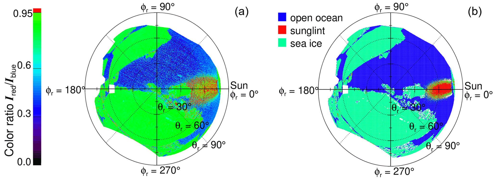
Figure 3(a) Color ratio of an exemplary scene (same scene as in Fig. 1d). The area identified as sunglint (above the color ratio threshold c=0.95) is highlighted in red. (b) Allocation of the pixels to sea ice (turquoise), open ocean (blue), or the sunglint area of open ocean (red) applying the sea ice mask illustrated in Fig. 4.
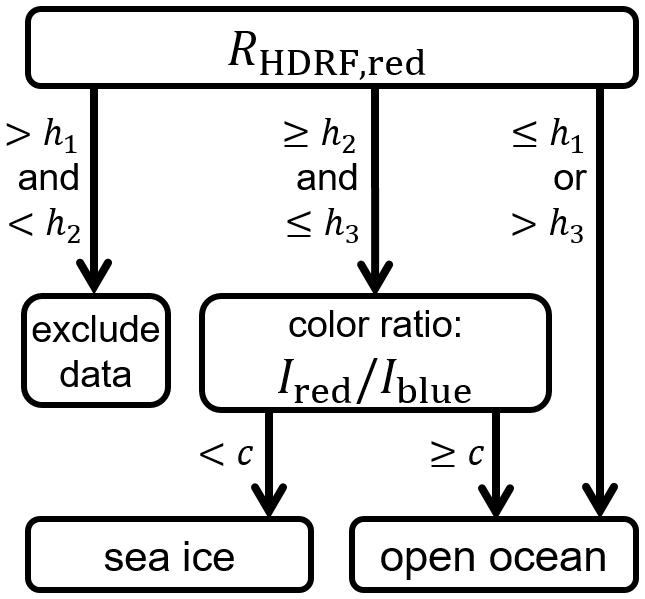
Figure 4Decision tree separating pixels covered by sea ice and open ocean, defining the sea ice mask. The applied thresholds h1=0.3, h2=0.6, and h3=1.3 are based on the HDRF retrieved for the red camera channel RHDRF,red. The threshold c=0.95 is based on the ratio of the radiances measured in the red Ired and the blue Iblue channel.
3.2 Sea ice fraction
Using the sea ice mask, the sea ice fraction was calculated for each image. The sea ice fraction refers to the portion of the total horizontal surface that is covered by ice. The fish-eye lens of the camera, however, weighs the individual pixels equally although each pixel refers to a different surface area. Nadir pixels cover a smaller area than pixels close to the horizon. These different pixel projections were taken into account when the sea ice fraction averaged over a whole image was calculated.
Within the analyzed time interval, the sea ice fraction varied between 0.35 and 1.0. The frequency distribution of the derived sea ice fraction is shown in black in Fig. 5. Images with higher sea ice fractions were more frequent than images dominated by open ocean. The dashed line indicates the mean sea ice fraction of 0.83 sampled during the 20 min measurement time interval. The accuracy of the sea ice fraction depends on the choice of the thresholds that are applied in the sea ice mask. In order to estimate the uncertainty related to the choice of the HDRF threshold values, a sensitivity study was performed, slightly varying one of the thresholds while the others were held constant. Two additional distributions, representing the lowest and the highest resulting sea ice fraction, are illustrated in Fig. 5.

Figure 5Frequency distribution of the sea ice fraction resulting from the applied sea ice mask for all images taken within the 20 min time interval (black) and for adapted sea ice masks (color-coded). The vertical dashed lines represent the resulting mean sea ice fraction.
The thresholds h1 and h2 were varied between the two modes (0.2 to 0.6). Changing h1 or h2 by 0.1 leads to a change in the sea ice fraction of about 1.2 %. h3 and the color ratio threshold c were varied between 1.2 and 1.4 and between 0.9 and 1.0, respectively. The sensitivity to the sea ice fraction is higher when h3 or c is decreased. However, the lower limits of both h3 and c were chosen such that the amount of obvious misclassification of sea ice as sunglint is limited. As is visible in Fig. 5, the averaged sea ice fraction resulting from the variation in the thresholds ranges between 0.79 and 0.86. Thus, the uncertainty in the sea ice fraction due to the sea ice mask is estimated to be less than 4 %.
Although the derived sea ice fraction slightly exceeds the upper limit of the MIZ definition given by Strong and Rigor (2013), the observations originate from an area very close to the sea ice edge and are characterized by separated and irregularly distributed ice floes typical of the MIZ.
After applying the sea ice mask to each of the images, all HDRF measurements of one single direction (pixel) assigned to either sea ice or open ocean were averaged. Doing so for all directions leads to a separated HDRF for each of the two surface types.
4.1 HDRF of open ocean
Figure 6a shows the average HDRF of the open-ocean areas separated from the observations in the MIZ (separated open-ocean HDRF). For most reflection directions the HDRF values are below 0.3. The average HDRF outside the sunglint region is 0.11 with an uncertainty of ±0.02 when different thresholds are applied in the sea ice mask algorithm. In the sunglint region (; ) the reflection is significantly enhanced and exceeds the maximum of the scale chosen here. A cross-section of the separated open-ocean HDRF along the solar principal plane is illustrated in Fig. 6b (blue line) and shows the full dynamic range of the sunglint with a maximum HDRF of around 9. The standard deviation (blue shading in Fig. 6b) is up to 0.6 outside the sunglint region and up to 9.2 in the sunglint region. The high standard deviation outside the sunglint results from misclassifications of sea ice as “sunglint”, which are, thus, assigned to open ocean. For each direction, the fraction of open-ocean pixels classified as sunglint (calculated as a ratio of all images) is referred to as the pixel-based sunglint fraction and indicated by the grey line in Fig. 6b. Even on the shadow side, about 10 % of the pixels are contributions of misclassified sunglint. Neglecting the sunglint criteria (h3 and c) would prevent these misclassifications and reduce the standard deviation to 0.11. Additionally, some of the observed variability results from the high sea ice fraction, which leads to a low number of open-ocean pixels in the entire data set. Although the pixel-based sea ice fraction (black line in Fig. 6b), which is derived similarly to the pixel-based sunglint fraction, is higher than 0.8 for most reflection directions, it also reveals significant directional variability.

Figure 6(a) Polar plot of the separated mean HDRF of open ocean. (b) Cross-section of the HDRF of open ocean along the solar principal plane (blue). The shaded area shows the standard deviation calculated for each direction of the solar principal plane from the entire time series (138 images). The black line denotes the mean pixel-based sea ice fraction (the portion of images where the respective pixel of the solar principal plane is assigned to sea ice). The grey line denotes the mean pixel-based sunglint fraction (the ratio of the number of images where the respective pixel of the solar principal plane is classified as sunglint to the number of images where this pixel is assigned to open ocean).
In the observations presented here, the sunglint does not have the shape of a typical Gaussian distribution as reported in the literature (e.g., Cox and Munk, 1954; Gatebe and King, 2016; Ehrlich et al., 2012). Instead, several smaller local maxima are obvious beside a global one and the sunglint is slurred towards the horizon. The irregular shape of the sunglint is likely a result of the low number of observations and is imprinted in the pixel-based sunglint fraction. It implies that the shape of the sunglint is highly variable among the images used for averaging, ranging from pure specular reflection of the Sun to sunglints cut by the edge of an ice floe (i.e., Fig. 1b) and widely blurred sunglints (i.e., Fig. 1d). The width of the sunglint primarily depends on the surface roughness, which is related to the surface wind speed (Cox and Munk, 1954). However, the distribution of sea ice and open ocean in the MIZ affects the surface roughness and its dependence on the wind speed. The development of waves is weaker in the gaps between ice floes than in the homogeneous open ocean (Kohout et al., 2011). This leads to the hypothesis that the shape, extent, and also position of the sunglint in the MIZ largely depend on the size of the open-ocean areas between the ice floes. The ice floe distribution differed significantly between the images, which might have caused the diversity of the sunglints observed in these measurements.
The dependence of wind speed and sunglint was tested by comparing the separated open-ocean HDRF to radiative transfer simulations. The simulated open-ocean HDRF was obtained from libRadtran, which incorporates BRDF parametrizations of different surface types (Mayer and Kylling, 2005) including open ocean (Cox and Munk, 1954). The simulations were performed for different wind speeds ranging from 1 m s−1 (minimum possible wind speed in libRadtran) to 10 m s−1. The atmospheric conditions were provided by measurements of a radiosonde launched at Ny-Ålesund at 12:00 UTC on 25 June 2017. Above, the default sub-Arctic summer atmosphere was selected. The solar zenith angle was set to 57.8∘, corresponding to the observation time. The hemispherical downward irradiance and the directional upward radiances at ground level (resolution 3∘ in the zenith direction and 5∘ in the azimuth direction) were simulated in a wavelength range between 350 and 750 nm and were converted into the spectral range of the red camera channel.
Cross-sections of the simulated open-ocean HDRF for several wind speeds are shown in Fig. 7. For low wind speeds, two local maxima of the open-ocean HDRF are visible, representing the sunglint (around the specular point) and the reflection of the diffuse incident radiation towards the horizon. With increasing wind speed, the sunglint distribution becomes broader while its maximum decreases in intensity and is shifted further to the horizon (e.g., Su et al., 2002). The HDRF peak at the horizon increases with increasing wind speed, which is likely due to an increase in diffuse incident radiation caused by multiple scattering between the sea surface and atmosphere. For wind speeds higher than about 3.5 m s−1, the diffuse reflection peak becomes dominant while the sunglint vanishes in its slope. The impact of the diffuse radiation (reflected skylight) on the BRDF and a method to remove this offset were discussed by Cox and Munk (1954). The black line in Fig. 7 represents the separated open-ocean HDRF. The airborne measurements of the wind speed were extrapolated to 10 m over the ground and amount to about 5 m s−1 on average. The comparison between the observation and the simulation for the observed wind speed shows that the maximum HDRF values and their positions do not coincide. Rather, the separated open-ocean HDRF reveals a larger sunglint peak, which is located closer to the specular point compared to the simulated open-ocean HDRF. The HDRF simulated with a wind speed of 1 m s−1 (or even less) compares better to the observations. Unfortunately, simulations with lower wind speeds were not supported by libRadtran. This indicates that the actual surface roughness of open ocean in the MIZ is significantly reduced because of the wave attenuation between the ice floes, leading to a narrower and more intense sunglint with its maximum closer to the specular point. The remaining discrepancy in the maximum HDRF between observation and simulation (1 m s−1) could be due to the limited data set (e. g., the variability in the sunglint shape) or the still too high wind speed. However, since similar differences for high SZAs have been observed by Su et al. (2002), this might also be an effect of the larger SZA compared to the original measurements by Cox and Munk (1954).
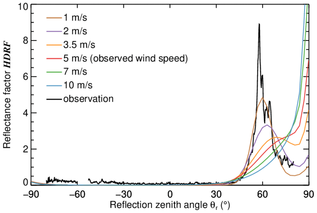
Figure 7Cross-sections of the open-ocean HDRF along the solar principal plane simulated with different wind speeds (color-coded) between 1 and 10 m s−1 including the observed wind speed of 5 m s−1. The black line corresponds to the separated open-ocean HDRF. The mean observed SZA also used for the simulation was 57.8∘.
Interestingly, the simulated open-ocean HDRF outside the sunglint is significantly lower than the separated one. Nearly independent of the wind speed, the mean simulated HDRF of the shadow side (90 to 270∘ reflection azimuth angle) is around 0.03, which is about 0.08 lower than for the separated HDRF. It is likely that these differences are due to horizontal photon transport. In the MIZ some photons reflected from the sea ice surface are scattered in the atmosphere such that they are detected in directions that actually point to open ocean as discussed by Schäfer et al. (2015). This effect may increase the HDRF of open ocean in the MIZ compared to homogeneous ice-free ocean.
4.2 HDRF of sea ice
Similarly to open ocean (Fig. 6), the average HDRF of the separated snow-covered sea ice areas (separated sea ice HDRF) is shown in Fig. 8. Note that the ranges of the y axes in Figs. 6b and 8b are different. In comparison to open ocean, the HDRF values are significantly higher for a large part of the angular domain with values around 0.9. The HDRF is slightly enhanced in the forward direction, which is obvious in both the polar plot (Fig. 8a) and the HDRF along the solar principal plane (Fig. 8b) and is in accordance with the literature (e.g., Bourgeois et al., 2006; Gatebe et al., 2003; Goyens et al., 2018). The maximum standard deviation below 0.2 reveals a lower variability compared to open ocean (0.6, including the misclassifications), which indicates that the mean sea ice HDRF is less affected by misclassified pixels.
Figure 8Same as Fig. 6 but for sea ice and without the mean pixel-based sea ice fraction and the mean pixel-based sunglint fraction in (b).
In order to assess potential differences between the HDRF of homogeneous snow-covered sea ice surfaces and sea ice areas in the inhomogeneous MIZ, the separated sea ice HDRF is compared to homogeneous sea ice and snow HDRFs obtained from two studies (Goyens et al., 2018; Carlsen et al., 2020). The ground-based fish-eye camera measurements described by Goyens et al. (2018) were performed on landfast sea ice in the southern Baffin Bay in May and June 2015. The HDRFs of three different sea ice surface types (bare ice, snow-covered ice, and ponded ice) were analyzed. The airborne observations made by Carlsen et al. (2020) were performed over homogeneous snow surfaces on the Antarctic Plateau in December 2013. The SZA during these measurements was similar to the SZA observed in our case study (about 58∘). The comparison of the HDRF along the solar principal plane is shown in Fig. 9.
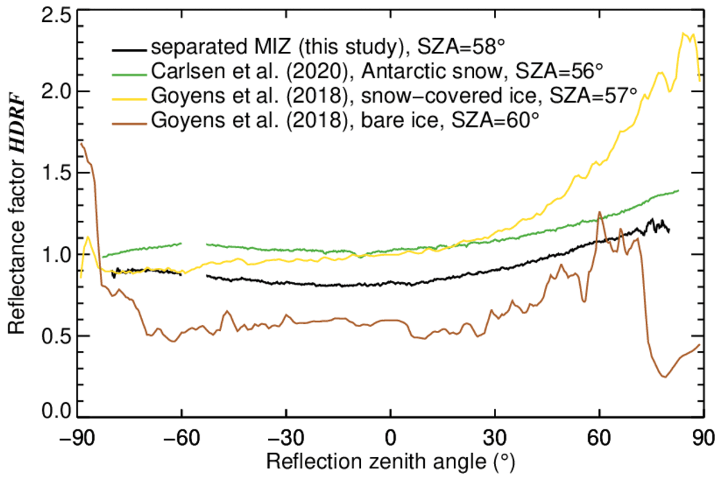
Figure 9Comparison of the cross-sections of the HDRF of snow, snow-covered, and bare sea ice along the solar principal plane obtained from different studies (color-coded); see text for details.
Compared to the separated sea ice HDRF (black line), the snow HDRF from Carlsen et al. (2020) has a similar shape but shows a higher magnitude for all reflection directions of the solar principal plane (0.19 at nadir). Likewise, the HDRF of snow-covered sea ice (yellow line) observed by Goyens et al. (2018) is larger than the separated sea ice HDRF (0.16 at nadir), except for with reflection zenith angles less than −60∘. However, comparing both snow HDRFs, significant differences in their anisotropies are obvious. While the anisotropy of the snow HDRF measured by Carlsen et al. (2020) is lower than that of the separated sea ice HDRF (the difference between both reduces to 0.12 at 59∘), the anisotropy is significantly larger for the snow-covered sea ice HDRF (Goyens et al., 2018) with a maximum difference from the separated sea ice HDRF of 0.95 at 77∘. In contrast to the other HDRF distributions with a minimum in the nadir-viewing direction, the minimum of the snow-covered sea ice HDRF by Goyens et al. (2018) is located in the backward direction (at about −60∘). The reasons for the anisotropy differences of both snow HDRFs (Carlsen et al., 2020; Goyens et al., 2018) remain unclear and might result from, e.g., snow grain size, impurity load, or surface roughness. While the measurements from Carlsen et al. (2020) were performed at a wavelength of 538 nm (green channel), the HDRFs at 628 nm (red channel) by Goyens et al. (2018) were used for comparison. However, the spectral dependence of the snow HDRF in the spectral range is small. The increased variability in the snow-covered sea ice HDRF observed by Goyens et al. (2018) might be due to the smaller footprint of the ground-based measurements compared to the airborne observations. In particular, small-scale surface roughness features can be resolved, which contribute to the variability in the ground-based measurements. In contrast to the snow-covered surfaces, the HDRF of bare ice (brown line) is significantly lower than the separated HDRF of the airborne observations and is characterized by an increased anisotropy. This is most prominent at reflection zenith angles of about 60∘. However, the shape of the bare-ice HDRF distribution is less smooth and shows a variability that is even larger than that of the snow-covered sea ice HDRF. According to Goyens et al. (2018), this is due to the presence of thawed ice near highly reflective ice grains, which often occurs at the beginning of the melt season.
The magnitude of the separated sea ice HDRF analyzed in this study ranges between the literature values for snow-covered and bare-ice HDRFs. This is reasonable since the observed ice floes revealed a mixture of snow-covered and bare ice (e.g., Fig. 1c). The comparison of the different HDRFs illustrates the variability in the snow and sea ice HDRF in polar environments, which is affected by a variety of properties (e.g., snow cover, snow grain size, or impurity concentration). Due to the significantly larger area fraction of sea ice compared to open ocean, the impact of the nearby darker open-ocean surfaces in terms of horizontal photon transport should be much smaller (<0.02) for sea ice and, thus, cannot completely explain the differences between the analyzed HDRFs.
In this section, the average HDRF of the inhomogeneous sea ice–open-ocean surface in the MIZ is compared to a constructed HDRF of the MIZ assuming a linear combination of the individual HDRFs of open ocean RHDRF,ocean and sea ice RHDRF,ice weighted by the sea ice fraction fice:
To do so, the data set was randomly split into two subsets. One of the subsets, the test data set, consists of 35 images (roughly 25 %) that are averaged without separation to obtain a mean HDRF of the inhomogeneous MIZ (mean MIZ HDRF). The sea ice fraction of this data set was calculated using the sea ice mask. The remaining subset, the separation data set, was used to separate and recombine the individual HDRFs into a constructed HDRF. The HDRF histograms of both subsets are shown in Fig. 10. The location of the modes of both data sets is similar to the distribution of the entire data set (black line). The open-ocean mode of the test data set is lower, while its sea ice mode is slightly shifted towards lower values. Nevertheless, the agreement of both data sets suggests that the same thresholds of the sea ice mask can be applied to all images. The sea ice fraction amounts to 0.83 and 0.81 for the separation and the test data set, respectively, with uncertainties of 4 % that are similar to the complete data set.
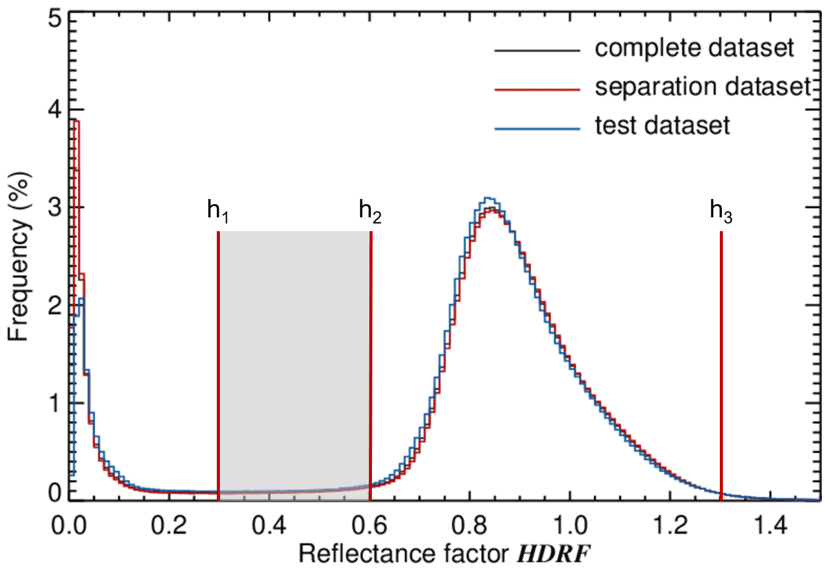
Figure 10Same as Fig. 2 but also including the distributions of the separation data set (red) and test data set (blue).
The mean MIZ HDRF from the test data set is illustrated in Fig. 11a. Despite the high sea ice fraction, the mean MIZ HDRF shows features of both open-ocean and sea ice surfaces. The strongly enhanced reflectance in the sunglint region is clearly visible. However, because of the high sea ice fraction, its maximum HDRF (about 3.0) is significantly lower compared to the separated open-ocean HDRF (see Fig. 6a). Outside the sunglint but still in the forward direction, the slightly enhanced HDRF characteristic for the sea ice surface is imprinted in the mean MIZ HDRF (compare Fig. 8a). For all other directions, the HDRF is more or less isotropic with values slightly lower (mean of 0.76 on the shadow side) than observed in the sea ice HDRF (0.90), due to the contribution of open-ocean surfaces.

Figure 11Polar plot of (a) the mean MIZ HDRF of the test data set (obtained by averaging over all images without separation) and (b) the constructed MIZ HDRF (calculated from the separated sea ice and open-ocean HDRFs of the separation data set according to Eq. 5 using a sea ice fraction of 0.83). (c) Cross-section of the constructed MIZ HDRF along the solar principal plane obtained from the separated HDRFs of the separation data set for different sea ice fractions fice (color-coded) and the mean MIZ HDRF of the test data set (black). (d) same as (c), but sea-ice-fraction-dependent simulations were used for the open-ocean HDRF; see text for details.
For comparison, the HDRF of the MIZ is constructed using Eq. (5). Firstly, it is tested whether the mean MIZ HDRF from the test data set can be reproduced. The MIZ HDRF is constructed using the separated open-ocean and sea ice HDRFs from the separation data set and the sea ice fraction of the test data set (0.81). The constructed HDRF is shown in Fig. 11b and compared to the mean MIZ HDRF (Fig. 11a). The difference between both HDRFs is less than 0.1 for 84 % of the pixels. The constructed MIZ HDRF appears more smoothed than the mean MIZ HDRF for statistical reasons. The smoothness was quantified by the standard deviation of the HDRF calculated with respect to all reflection directions of the shadow side (to exclude the sunglint contribution). For the constructed MIZ HDRF the standard deviation is slightly lower (0.03, 4.3 % of the mean value) than for the mean MIZ HDRF (0.05, 6.5 % of the mean value). The smoothness for the constructed HDRF is due to the assumption of a homogeneous and uniform sea ice fraction in Eq. (5), whereas the measured mean HDRF is affected by the directionally inhomogeneous sea ice fraction and the quite low number of images included in the test data set. Figure 12 illustrates the variability in the pixel-based sea ice fraction of the test data set. It is obvious that for each pixel the pixel-based sea ice fraction is different, covering a wide range between 0.5 and 1.0. Increasing the number of images (which could be reached by, e.g., increasing the sampling frequency, currently Hz) would reduce such effects, and the pixel-based sea ice fraction would become more homogeneous.
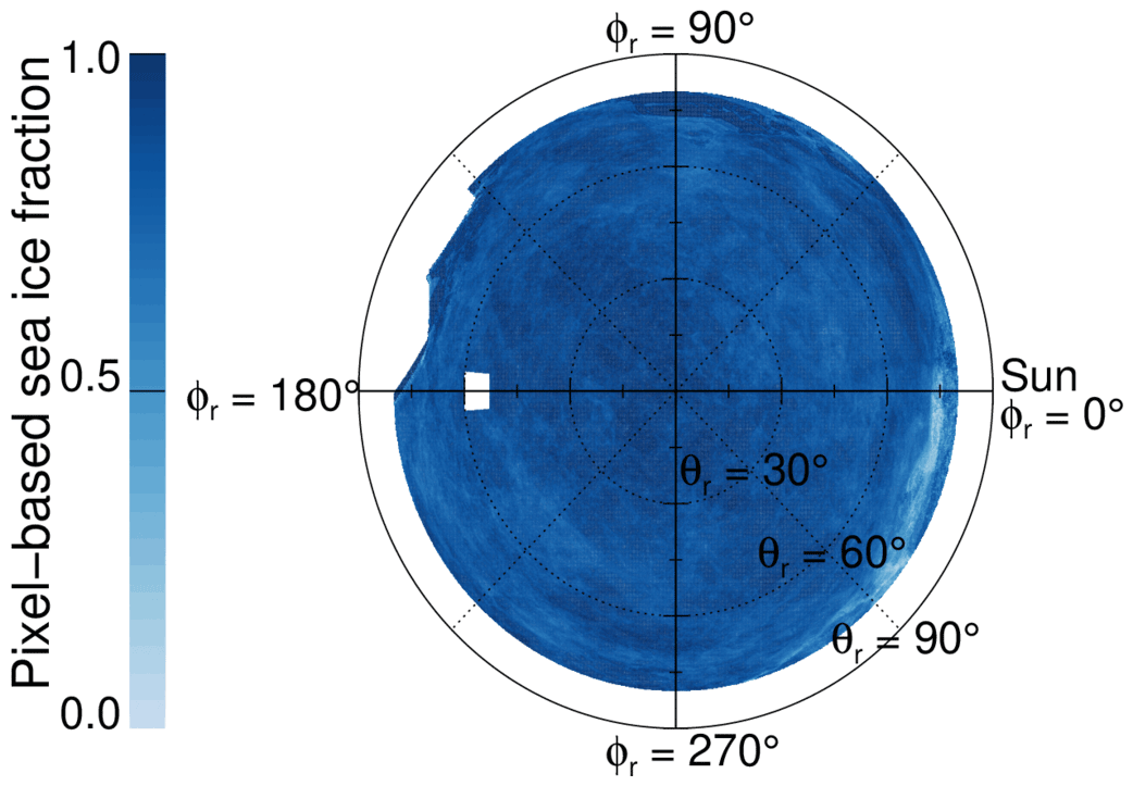
Figure 12Sea ice fraction observed at each pixel throughout the images used for the test data set (pixel-based sea ice fraction).
Figure 11c and d show cross-sections of the constructed MIZ HDRF along the solar principal plane for different sea ice fractions. In Fig. 11c the individual sea ice and open-ocean HDRFs separated from the separation data set are combined for different sea ice fractions. The open-ocean and sea ice HDRFs are represented by the sea ice fractions of 0 and 1, respectively. While the HDRF outside the sunglint increases with increasing sea ice fraction, the sunglint contribution decreases without changing its shape. However, as shown in Fig. 7, there is a significant mismatch between the open-ocean HDRF in the MIZ and that of the ice-free ocean due to wave attenuation. In Fig. 11c, the constructed HDRF for all sea ice fractions was retrieved using the MIZ open-ocean HDRF (sea ice fraction of 0.83). To assess the impact of the surface roughness on the constructed HDRF, in Fig. 11d, RHDRF,ocean is replaced by a simulated HDRF that depends on the surface roughness varying with fice. The simulations are performed in the same way as described in Sect. 4.1 except that the input surface wind speed veff is parametrized as a linear function of the sea ice fraction:
veff is considered an effective wind speed that would produce the same surface roughness and, thus, the same open-ocean HDRF if the ocean were ice-free. vmeas is the wind speed measured at flight altitude and extrapolated to 10 m altitude. It has to be noted that this very basic relation between the surface wind speed and sea ice fraction aims only to illustrate the effects in a qualitative view. Numbers may change if observations for different sea ice conditions are considered. The comparison of Fig. 11c and d reveals significant differences in the shape and the position of the sunglint. With a decreasing sea ice fraction, the increasing effective wind speed (Eq. 6) causes a shift of the sunglint towards the horizon (compare Fig. 7 with Fig. 11d). Furthermore, the irregular shape and sharp peak visible in Fig. 11c is not present in the smooth simulations. This also leads to a reduced HDRF maximum in Fig. 11d. Nevertheless, the comparison of either of the constructed HDRFs (Fig. 11c or d) for the sea ice fraction observed in the test data set (0.81, purple line) to its mean MIZ HDRF (black line) reveals only small differences outside the sunglint. The HDRF constructed with the simulated open-ocean HDRF (Fig. 11d) even shows good agreement with the mean MIZ HDRF at the sunglint slope. In total, the difference between both HDRFs is less than 0.1 for about 82 % of the directions of the solar principal plane.
This analysis has shown that the linear construction of the HDRF from individual HDRFs of open ocean and sea ice is well applicable if the environmental conditions are considered correctly. That also includes the parametrization of the surface roughness of the open ocean (effective surface wind speed), which considerably depends on the sea ice distribution. Neglecting those effects can lead to substantial irregularities in the resulting sunglint position and intensity.
Reflected radiance measurements were collected by an airborne 180∘ fish-eye camera in the MIZ north of Svalbard in June 2017. From these data, the HDRF was calculated during cloud-free conditions for a 20 min sequence of 138 camera images covering different sea ice fractions. The HDRFs of sea ice and open-ocean surfaces were separated by applying a sea ice mask with different reflectivity and color ratio thresholds.
From the separated images, the averaged HDRFs of open-ocean and partly snow-covered sea ice surfaces in the MIZ were derived. They confirmed the general features of open ocean and sea ice reported in the literature (e.g., Warren et al., 1998; Gatebe et al., 2003; Jackson and Alpers, 2010). However, a comparison with simulations indicated that the common BRDF parametrizations for homogeneous open-ocean surfaces as a function of the wind speed (Cox and Munk, 1954) partly differ in the MIZ. This is mainly due to wave attenuation between the ice floes in the MIZ (Kohout et al., 2011) leading to reduced surface roughness compared to a homogeneous open-ocean surface with the same surface wind speed. This effect narrows the sunglint and intensifies its magnitude. The irregular shape of the sunglint observed in the data set was a result of the limitation of the sunglint mask and the highly variable surface roughness associated with the irregular distribution of sea ice and open ocean in the MIZ.
The separated HDRF of partly snow-covered sea ice ranged between independent literature HDRFs of homogeneous snow and bare-ice surfaces. However, the comparison also revealed the large diversity of snow/sea ice HDRF patterns associated with the variability in snow and ice properties. Minor differences between the HDRF in the MIZ and that of homogeneous surfaces could originate as a result of the radiative effects of the contrasting surface type nearby (e.g., Ricchiazzi and Gautier, 1998; Schäfer et al., 2015).
The averaged HDRF of the MIZ showed features of both sea ice and open-ocean surfaces. Even for rather high sea ice fractions, there is still a contribution from the sunglint in the MIZ, which might affect the analysis of satellite observations in these reflection angles. This especially holds true with respect to the presence of leads in Arctic (e.g., Ivanova et al., 2016).
The mean MIZ HDRF of a subset of the analyzed data set was compared to the constructed one, calculated as a linear combination of the separated HDRFs of the remaining subset weighted by the sea ice fraction. The comparison showed good agreement for the measured sea ice fraction with a difference of less than 0.1 for 84 % of the pixels. Due to the assumption of a directionally constant sea ice fraction, the constructed HDRF of the MIZ was found to be smoother than the mean MIZ HDRF. Altogether, this analysis implies that the construction of the MIZ HDRF from individual sea ice and open-ocean HDRFs provides meaningful results. This approach could become relevant for randomly distributed sea ice and open ocean where only the sea ice fraction is known.
However, the impact of the wave attenuation on the open-ocean HDRF in the MIZ also has a significant impact on the sunglint pattern of the mean MIZ HDRF. This effect needs to be considered in retrieval methods similar to the one used here. To improve the applicability of such methods, further research is needed regarding the parametrization of the surface roughness of open ocean in the MIZ. Also the impact of the exact floe distribution on the surface reflectance properties needs to be investigated further. To extend the method to different environmental conditions (e.g., sea ice fraction, surface wind speed), further measurements are needed for a full parametrization of the HDRF in such complex scenarios as the MIZ, which may be the dominant surface type of the future Arctic.
All data measured by the research aircraft Polar 5 during ACLOUD and used in this study are published on the PANGAEA database. The radiances measured by the digital camera equipped with a fish-eye lens can be found at https://doi.org/10.1594/PANGAEA.901024 (Jäkel and Ehrlich, 2019). The spectral irradiance data measured by SMART were published by Jäkel et al. (2019a, https://doi.org/10.1594/PANGAEA.899177). The wind speed was published together with other meteorological parameters (Hartmann et al., 2019, https://doi.org/10.1594/PANGAEA.902849). The radiosounding used for radiative transfer simulations is available in Maturilli (2017, https://doi.org/10.1594/PANGAEA.879822). The HDRF data described by Goyens et al. (2018, https://doi.org/10.1002/2017EA000332) can be found on SEANOE (Goyen et al., 2015; https://doi.org/10.17882/55352).
All authors contributed to the discussion of the results and the editing of the article. SB selected the case study, analyzed the data, and drafted the article. SB developed the sea ice mask and performed the radiative transfer simulations. AE initiated the study. EJ processed the radiance and irradiance data. MW and AE designed the experimental basis of this study.
The contact author has declared that neither they nor their co-authors have any competing interests.
Publisher's note: Copernicus Publications remains neutral with regard to jurisdictional claims in published maps and institutional affiliations.
This article is part of the special issue “Arctic mixed-phase clouds as studied during the ACLOUD/PASCAL campaigns in the framework of (AC)3 (ACP/AMT/ESSD inter-journal SI)”. It is not associated with a conference.
We gratefully acknowledge the funding by the Deutsche Forschungsgemeinschaft (DFG, German Research Foundation) – Projektnummer 268020496 – TRR 172, within the Transregional Collaborative Research Center “ArctiC Amplification: Climate Relevant Atmospheric and SurfaCe Processes, and Feedback Mechanisms (AC)3”.
This research has been supported by the Deutsche Forschungsgemeinschaft (grant no. 268020496).
This paper was edited by Jost Heintzenberg and reviewed by two anonymous referees.
Aoki, T., Aoki, T., Fukabori, M., Hachikubo, A., Tachibana, Y., and Nishio, F.: Effects of snow physical parameters on spectral albedo and bidirectional reflectance of snow surface, J. Geophys. Res.-Atmos., 105, 10219–10236, https://doi.org/10.1029/1999JD901122, 2000. a
Bierwirth, E., Wendisch, M., Ehrlich, A., Heese, B., Tesche, M., Althausen, D., Schladitz, A., Mueller, D., Otto, S., Trautmann, T., Dinter, T., von Hoyningen-Huene, W., and Kahn, R.: Spectral surface albedo over Morocco and its impact on radiative forcing of Saharan dust, Tellus B, 61, 252–269, https://doi.org/10.1111/j.1600-0889.2008.00395.x, 2009. a
Bourgeois, C. S., Ohmura, A., Schroff, K., Frei, H.-J., and Calanca, P.: IAC ETH goniospectrometer: A tool for hyperspectral HDRF measurements, J. Atmos. Ocean. Tech., 23, 573–584, https://doi.org/10.1175/JTECH1870.1, 2006. a, b, c, d
Carlsen, T., Birnbaum, G., Ehrlich, A., Helm, V., Jäkel, E., Schäfer, M., and Wendisch, M.: Parameterizing anisotropic reflectance of snow surfaces from airborne digital camera observations in Antarctica, The Cryosphere, 14, 3959–3978, https://doi.org/10.5194/tc-14-3959-2020, 2020. a, b, c, d, e, f, g, h, i, j, k, l
Cox, C. and Munk, W.: Measurement of the roughness of the sea surface from photographs of the sun's glitter, J. Opt. Soc. Am. A, 44, 838–850, 1954. a, b, c, d, e, f, g, h, i
Ehrlich, A., Bierwirth, E., Wendisch, M., Herber, A., and Gayet, J.-F.: Airborne hyperspectral observations of surface and cloud directional reflectivity using a commercial digital camera, Atmos. Chem. Phys., 12, 3493–3510, https://doi.org/10.5194/acp-12-3493-2012, 2012. a, b, c
Ehrlich, A., Wendisch, M., Lüpkes, C., Buschmann, M., Bozem, H., Chechin, D., Clemen, H.-C., Dupuy, R., Eppers, O., Hartmann, J., Herber, A., Jäkel, E., Järvinen, E., Jourdan, O., Kästner, U., Kliesch, L.-L., Köllner, F., Mech, M., Mertes, S., Neuber, R., Ruiz-Donoso, E., Schnaiter, M., Schneider, J., Stapf, J., and Zanatta, M.: A comprehensive in situ and remote sensing data set from the Arctic CLoud Observations Using airborne measurements during polar Day (ACLOUD) campaign, Earth Syst. Sci. Data, 11, 1853–1881, https://doi.org/10.5194/essd-11-1853-2019, 2019. a, b, c, d
Emde, C., Buras-Schnell, R., Kylling, A., Mayer, B., Gasteiger, J., Hamann, U., Kylling, J., Richter, B., Pause, C., Dowling, T., and Bugliaro, L.: The libRadtran software package for radiative transfer calculations (version 2.0.1), Geosci. Model Dev., 9, 1647–1672, https://doi.org/10.5194/gmd-9-1647-2016, 2016. a
Feng, Y., Liu, Q., Qu, Y., and Liang, S.: Estimation of the Ocean Water Albedo From Remote Sensing and Meteorological Reanalysis Data, IEEE T. Geosci. Remote, 54, 850–868, https://doi.org/10.1109/TGRS.2015.2468054, 2016. a
Gatebe, C. K. and King, M. D.: Airborne spectral BRDF of various surface types (ocean, vegetation, snow, desert, wetlands, cloud decks, smoke layers) for remote sensing applications, Remote Sens. Environ., 179, 131–148, https://doi.org/10.1016/j.rse.2016.03.029, 2016. a
Gatebe, C., King, M., Platnick, S., Arnold, G., Vermote, E., and Schmid, B.: Airborne spectral measurements of surface-atmosphere anisotropy for several surfaces and ecosystems over southern Africa, J. Geophys. Res., 108, 8489, https://doi.org/10.1029/2002JD002397, 2003. a, b, c, d
Gatebe, C. K., King, M. D., Lyapustin, A. I., Arnold, G. T., and Redemann, J.: Airborne spectral measurements of ocean directional reflectance, J. Atmos. Sci., 62, 1072–1092, 2005. a
Goyens, C., Marty, S., Leymarie, E., Antoine, D., Babin, M., and Bélanger, S.: High angular and spectral directional reflectance dataset of snow and sea-ice, SEANOE [data set], https://doi.org/10.17882/55352, 2015. a
Goyens, C., Marty, S., Leymarie, E., Antoine, D., Babin, M., and Bélanger, S.: High Angular Resolution Measurements of the Anisotropy of Reflectance of Sea Ice and Snow, Earth Space Sci., 5, 30–47, https://doi.org/10.1002/2017EA000332, 2018. a, b, c, d, e, f, g, h, i, j, k, l
Hartmann, J., Lüpkes, C., and Chechin, D.: 1Hz resolution aircraft measurements of wind and temperature during the ACLOUD campaign in 2017, Alfred Wegener Institute, Helmholtz Centre for Polar and Marine Research, Bremerhaven, PANGAEA [data set], https://doi.org/10.1594/PANGAEA.902849, 2019. a
Hoffman, J. P., Ackerman, S. A., Liu, Y., and Key, J. R.: The Detection and Characterization of Arctic Sea Ice Leads with Satellite Imagers, Remote Sens., 11, 521, https://doi.org/10.3390/rs11050521, 2019. a
Ivanova, N., Rampal, P., and Bouillon, S.: Error assessment of satellite-derived lead fraction in the Arctic, The Cryosphere, 10, 585–595, https://doi.org/10.5194/tc-10-585-2016, 2016. a
Jackson, C. and Alpers, W.: The role of the critical angle in brightness reversals on sunglint images of the sea surface, J. Geophys. Res., 115, C09019, https://doi.org/10.1029/2009JC006037, 2010. a, b
Jafariserajehlou, S., Rozanov, V. V., Vountas, M., Gatebe, C. K., and Burrows, J. P.: Simulated reflectance above snow constrained by airborne measurements of solar radiation: implications for the snow grain morphology in the Arctic, Atmos. Meas. Tech., 14, 369–389, https://doi.org/10.5194/amt-14-369-2021, 2021. a
Jäkel, E. and Ehrlich, A.: Radiance fields of clouds and the Arctic surface measured by a digital camera during ACLOUD 2017, Leipzig Institute for Meteorology, University of Leipzig, PANGAEA [data set], https://doi.org/10.1594/PANGAEA.901024, 2019. a, b
Jäkel, E., Ehrlich, A., Schäfer, M., and Wendisch, M.: Aircraft measurements of spectral solar up- and downward irradiances in the Arctic during the ACLOUD campaign 2017, Universität Leipzig, PANGAEA [data set], https://doi.org/10.1594/PANGAEA.899177, 2019a. a, b
Jäkel, E., Stapf, J., Wendisch, M., Nicolaus, M., Dorn, W., and Rinke, A.: Validation of the sea ice surface albedo scheme of the regional climate model HIRHAM–NAOSIM using aircraft measurements during the ACLOUD/PASCAL campaigns, The Cryosphere, 13, 1695–1708, https://doi.org/10.5194/tc-13-1695-2019, 2019b. a
Jiang, K.: Calibrate fisheye lens using OpenCV – part 1, https://medium.com/@kennethjiang/calibrate-fisheye-lens-using-opencv-333b05afa0b0 (last access: 18 August 2020), 2017. a
Jin, Z., Charlock, T., Smith, W., and Rutledge, K.: A parameterization of ocean surface albedo, Geophys. Res. Lett., 31, L22301, https://doi.org/10.1029/2004GL021180, 2004. a
Kashiwase, H., Ohshima, K. I., Nihashi, S., and Eicken, H.: Evidence for ice-ocean albedo feedback in the Arctic Ocean shifting to a seasonal ice zone, Sci. Rep., 7, 8170, https://doi.org/10.1038/s41598-017-08467-z, 2017. a
Kohout, A. L., Meylan, M. H., and Plew, D. R.: Wave attenuation in a marginal ice zone due to the bottom roughness of ice floes, Ann. Glaciol., 52, 118–122, https://doi.org/10.3189/172756411795931525, 2011. a, b, c
Kwok, R.: Arctic sea ice thickness, volume, and multiyear ice coverage: losses and coupled variability (1958–2018), Environ. Res. Lett., 13, 105005, https://doi.org/10.1088/1748-9326/aae3ec, 2018. a
Marks, A., Fragiacomo, C., MacArthur, A., Zibordi, G., Fox, N., and King, M. D.: Characterisation of the HDRF (as a proxy for BRDF) of snow surfaces at Dome C, Antarctica, for the inter-calibration and inter-comparison of satellite optical data, Remote Sens. Environ., 158, 407–416, https://doi.org/10.1016/j.rse.2014.11.013, 2015. a
Maturilli, M.: High resolution radiosonde measurements from station Ny-Ålesund (2017-06), Alfred Wegener Institute – Research Unit Potsdam, PANGAEA [data set], https://doi.org/10.1594/PANGAEA.879822, 2017. a
Mayer, B. and Kylling, A.: Technical note: The libRadtran software package for radiative transfer calculations – description and examples of use, Atmos. Chem. Phys., 5, 1855–1877, https://doi.org/10.5194/acp-5-1855-2005, 2005. a, b
Nicodemus, F., Richmond, J., Hsia, J., Ginsber, I. W., and Limperis, T.: Geometrical Considerations and Nomenclature for Reflectance, NBS Monograph, vol. 160, US Department of Commerce, National Bureau of Standards, Washington, D.C., 1977. a, b
Perovich, D., Meier, W., Tschudi, M., Farrell, S., Hendricks, S., Gerlach, S., Haas, C., Krumpen, T., Polashenski, C., Ricker, R., and Webster, M.: Sea Ice, in: Arctic Report Card 2018, 25–32, https://arctic.noaa.gov/Report-Card/Report-Card-2018 (last access: 4 May 2022), 2018. a
Pithan, F. and Mauritsen, T.: Arctic amplification dominated by temperature feedbacks in contemporary climate models, Nature, 7, 181–184, https://doi.org/10.1038/ngeo2071, 2014. a
Qu, Y., Liang, S., Liu, Q., Li, X., Feng, Y., and Liu, S.: Estimating Arctic sea-ice shortwave albedo from MODIS data, Remote Sens. Environ., 186, 32–46, https://doi.org/10.1016/j.rse.2016.08.015, 2016. a
Ricchiazzi, P. and Gautier, C.: Investigation of the effect of surface heterogeneity and topography on the radiation environment of Palmer Station, Antarctica, with a hybrid 3-D radiative transfer model, J. Geophys. Res.-Atmos., 103, 6161–6176, https://doi.org/10.1029/97jd03629, 1998. a
Rolph, R. J., Feltham, D. L., and Schröder, D.: Changes of the Arctic marginal ice zone during the satellite era, The Cryosphere, 14, 1971–1984, https://doi.org/10.5194/tc-14-1971-2020, 2020. a
Schaaf, C. B., Gao, F., Strahler, A. H., Lucht, W., Li, X. W., Tsang, T., Strugnell, N. C., Zhang, X. Y., Jin, Y. F., Muller, J. P., Lewis, P., Barnsley, M., Hobson, P., Disney, M., Roberts, G., Dunderdale, M., Doll, C., d'Entremont, R. P., Hu, B. X., Liang, S. L., Privette, J. L., and Roy, D.: First operational BRDF, albedo nadir reflectance products from MODIS, Remote Sens. Environ., 83, 135–148, 2002. a
Schaepman-Strub, G., Schaepman, M. E., Painter, T. H., Dangel, S., and Martonchik, J. V.: Reflectance quantities in optical remote sensing-definitions and case studies, Remote Sens. Environ., 103, 27–42, 2006. a, b
Schäfer, M., Bierwirth, E., Ehrlich, A., Jäkel, E., and Wendisch, M.: Airborne observations and simulations of three-dimensional radiative interactions between Arctic boundary layer clouds and ice floes, Atmos. Chem. Phys., 15, 8147–8163, https://doi.org/10.5194/acp-15-8147-2015, 2015. a, b
Stapf, J., Ehrlich, A., Jäkel, E., Lüpkes, C., and Wendisch, M.: Reassessment of shortwave surface cloud radiative forcing in the Arctic: consideration of surface-albedo–cloud interactions, Atmos. Chem. Phys., 20, 9895–9914, https://doi.org/10.5194/acp-20-9895-2020, 2020. a
Strong, C. and Rigor, I. G.: Arctic marginal ice zone trending wider in summer and narrower in winter, Geophys. Res. Lett., 40, 4864–4868, https://doi.org/10.1002/grl.50928, 2013. a, b, c
Su, W., Charlock, T., and Rutledge, K.: Observations of relectance distribution around sunglint from a coastal ocean platform, Appl. Opt., 41, 7369–7383, 2002. a, b
Urquhart, B., Kurtz, B., and Kleissl, J.: Sky camera geometric calibration using solar observations, Atmos. Meas. Tech., 9, 4279–4294, https://doi.org/10.5194/amt-9-4279-2016, 2016. a
Warren, S., Brandt, R., and Hinton, P.: Effect of surface roughness on bidirectional reflectance of Antarctic snow, J. Geophys. Res.-Planets, 103, 25789–25807, https://doi.org/10.1029/98JE01898, 1998. a, b
Wendisch, M., Müller, D., Schell, D., and Heintzenberg, J.: An airborne spectral albedometer with active horizontal stabilization, J. Atmos. Ocean. Tech., 18, 1856–1866, https://doi.org/10.1175/1520-0426(2001)018<1856:AASAWA>2.0.CO;2, 2001. a
Wendisch, M., Brückner, M., Burrows, J. P., Crewell, S., Dethloff, K., Ebell, K., Lüpkes, C., Macke, A., Notholt, J., Quaas, J., Rinke, A., and Tegen, I.: Understanding causes and effects of rapid warming in the Arctic, Eos, 98, 22–26, https://doi.org/10.1029/2017EO064803, 2017. a
Wendisch, M., Macke, A., Ehrlich, A., Lüpkes, C., Mech, M., Chechin, D., Dethloff, K., Velasco, C. B., Bozem, H., Brückner, M., Clemen, H.-C., Crewell, S., Donth, T., Dupuy, R., Ebell, K., Egerer, U., Engelmann, R., Engler, C., Eppers, O., Gehrmann, M., Gong, X., Gottschalk, M., Gourbeyre, C., Griesche, H., Hartmann, J., Hartmann, M., Heinold, B., Herber, A., Herrmann, H., Heygster, G., Hoor, P., Jafariserajehlou, S., Jäkel, E., Järvinen, E., Jourdan, O., Kästner, U., Kecorius, S., Knudsen, E. M., Köllner, F., Kretzschmar, J., Lelli, L., Leroy, D., Maturilli, M., Mei, L., Mertes, S., Mioche, G., Neuber, R., Nicolaus, M., Nomokonova, T., Notholt, J., Palm, M., van Pinxteren, M., Quaas, J., Richter, P., Ruiz-Donoso, E., Schäfer, M., Schmieder, K., Schnaiter, M., Schneider, J., Schwarzenböck, A., Seifert, P., Shupe, M. D., Siebert, H., Spreen, G., Stapf, J., Stratmann, F., Vogl, T., Welti, A., Wex, H., Wiedensohler, A., Zanatta, M., and Zeppenfeld, S.: The Arctic Cloud Puzzle: Using ACLOUD/PASCAL Multiplatform Observations to Unravel the Role of Clouds and Aerosol Particles in Arctic Amplification, B. Am. Meteorol. Soc., 100, 841–871, https://doi.org/10.1175/BAMS-D-18-0072.1, 2019. a
Wesche, C., Steinhage, D., and Nixdorf, U.: Polar aircraft Polar5 and Polar6 operated by the Alfred Wegener Institute, J. Large-Scale Res. Facilities, 2, A87, https://doi.org/10.17815/jlsrf-2-153, 2016. a
Wiscombe, W.: Improved Mie scattering algorithms, Appl. Optics, 19, 1505–1509, 1980. a
- Abstract
- Introduction
- Methodology and measurements
- Separation of sea ice and open-ocean surfaces
- Separated HDRF and comparison with simulations and observations from the literature
- HDRF of the MIZ as a function of sea ice fraction
- Conclusions
- Data availability
- Author contributions
- Competing interests
- Disclaimer
- Special issue statement
- Acknowledgements
- Financial support
- Review statement
- References