the Creative Commons Attribution 4.0 License.
the Creative Commons Attribution 4.0 License.
 | 20 Jan 2022
Total water vapour columns derived from Sentinel 5P using the AMC-DOAS method
Tobias Küchler
Stefan Noël
Heinrich Bovensmann
John Philip Burrows
Thomas Wagner
Christian Borger
Tobias Borsdorff
Andreas Schneider
Water vapour is the most abundant natural greenhouse gas in the Earth's atmosphere, and global data sets are required for meteorological applications and climate research. The Tropospheric Monitoring Instrument (TROPOMI) on board Sentinel-5 Precursor (S5P) launched on 13 October 2017 has a high spatial resolution of around 5 km and a daily global coverage. Currently, there is no operational total water vapour product for S5P measurements. Here, we present first results of a new scientific total column water vapour (TCWV) product for S5P using the so-called air-mass-corrected differential optical absorption spectroscopy (AMC-DOAS) scheme. This method analyses spectral data between 688 and 700 nm and has already been successfully applied to measurements from the Global Monitoring Experiment (GOME) on ERS-2, the SCanning Imaging Absorption spectroMeter for Atmospheric CHartographY (SCIAMACHY) on Envisat and GOME-2 on MetOp.
The adaptation of the AMC-DOAS method to S5P data requires an additional post-processing procedure to correct the influences of surface albedo, cloud height and cloud fraction. The quality of the new AMC-DOAS S5P water vapour product is assessed by comparisons with data from GOME-2 on MetOp-B retrieved also with the AMC-DOAS algorithm and with four independent data sets, namely reanalysis data from the European Centre for Medium range Weather Forecast (ECMWF ERA5), data obtained by the Special Sensor Microwave Imager and Sounder (SSMIS) flown on the Defense Meteorological Satellite Program (DMSP) platform 16 and two scientific S5P TCWV products derived from TROPOMI measurements. Both are recently published TCWV products for S5P provided by the Max Planck Institute for Chemistry (MPIC) in Mainz and the Netherlands Institute for Space Research (SRON), Utrecht. The SRON TCWV is limited to clear-sky scenes over land.
These comparisons reveal a good agreement between the various data sets but also some systematic differences between all of them. On average, the daily derived offset between AMC-DOAS S5P TCWV and AMC-DOAS GOME-2B TCWV is negative (around −1.5 kg m−2) over land and positive over ocean surfaces (more than 1.5 kg m−2). In contrast, SSMIS TCWV is on average lower than AMC-DOAS S5P TCWV by about 3 kg m−2.
Monthly averaged ERA5 TCWV and AMC-DOAS S5P TCWV comparison shows spatial features over both land and water surface. Over land, there are systematic spatial structures. There are larger differences between AMC-DOAS S5P TCWV and ERA5 TCWV in tropical regions. Over sea, AMC-DOAS S5P TCWV is slightly lower than ERA5 TCWV by around 2 kg m−2. The AMC-DOAS S5P TCWV and S5P TCWV from MPIC agree on average within 1 kg m−2 over both land and ocean. TCWV from SRON shows daily global averaged differences to AMC-DOAS S5P TCWV of around 1.2 kg m−2. All of these differences are in line with the accuracy of these products and with the typical range of differences of 5 kg m−2 obtained when comparing different TCWV data sets.
The AMC-DOAS TCWV product for S5P provides therefore a valuable new and independent data set for atmospheric applications which also has a higher spatial coverage than the other S5P TCWV products.
- Article
(22722 KB) - Full-text XML
- BibTeX
- EndNote


As the most abundant natural greenhouse gas, water vapour has a strong impact on the energy balance of the atmosphere. Its absorption of the upwelling thermal infrared radiation from the Earth and the incoming solar radiation warms the atmosphere. Water vapour has a greenhouse heating effect twice as strong as carbon dioxide (Mitchell, 1989; Kiehl and Trenberth, 1997). Water vapour evaporates from the ocean, terrestrial fresh water, vegetation and moist soil. When it condenses in the atmosphere to form clouds, it releases latent heat.
The amount of water vapour in the atmosphere is limited by the saturated vapour pressure, which depends on the temperature. Thus changes in temperature will result in an altered water vapour loading. An increasing atmospheric temperature leads to an increase in water vapour saturation pressure, which is given by the Clausius–Clapeyron equation. In a warming climate, there is more evaporation, and thus the water vapour content in the atmosphere increases. This leads to a stronger absorption of outgoing longwave radiation, emitted from the Earth's surface, and to an increase of temperature in the atmosphere. However, the scattering of the incoming solar electromagnetic radiation by clouds cools the surface (Boucher et al., 2013). Overall this feedback mechanism is complex. Enhanced water vapour amounts will also affect the amount and strength of precipitation. As a consequence, the strength or amplitude of the hydrological cycle is also affected (Allan et al., 2014). Water vapour also plays an important role in atmospheric chemistry. In the atmosphere it is a source of the most important oxidizing agent, the free radical hydroxyl, OH.
In summary, to understand the physics and chemistry of the atmosphere, the changing hydrological cycle and climate, it is essential to know the global distribution of water vapour and its changes with time.
One of the most accurate methods to determine water vapour concentrations are in situ measurements from radiosondes, which provide atmospheric profiles of various atmospheric constituents at selected locations. These sites are distributed globally, but most of them are on land. However, radiosondes measure local conditions, and any network of such sondes is intrinsically sparse. The latter cannot fully capture the high spatial and temporal variability of water vapour from the local to the global scale.
Total column water vapour (TCWV) is also retrieved using the Global Positioning System (GPS) satellite signals in combination with local GPS ground stations (Bevis et al., 1992; Rocken et al., 1993, 1995). One advantage is the temporal high resolution. They yield TCWV for all weather conditions. In contrast, the spatial coverage is quite poor due to the limited number of ground-based receivers.
Another important part of the global observing system for water vapour is measurements made from passive remote sounding sensors from polar and geostationary orbiting platforms. These potentially provide global information about the atmosphere having full global coverage every day or better, dependent on the number of platforms flying simultaneously. This information can be used to fill the spatial and temporal gaps of the different ground-based measurements. A variety of possible methods to derive the total water vapour amount from space have been developed for various spectral regions.
One of the earliest TCWV data sets provided by satellites was derived from measurements in the microwave region by Nimbus 5 on NOAA (e. g. Staelin et al., 1976). In the same spectral region, the SSM/I instrument and its successor SSMIS on different platforms have provided the longest TCWV time series from 1987 up to now. The measurements of microwave sounders yield water vapour under cloud-free and cloudy conditions. These data products are usually limited to those measurements made above water surface. With microwave sounders, it is possible to retrieve water vapour under cloud-free and cloudy conditions, but the retrievals are usually restricted to water surfaces due to contributions of land surface emissions to the received signal that are not well known (Schlüssel and Emery, 1990; Wentz, 1997). However, Melsheimer and Heygster (2008) extended the microwave retrieval to polar regions, where ice and snow is present throughout the year.
TCWV retrievals are also possible in the thermal infrared spectral region, for example, by the mathematical inversion of measurements from Infrared Atmospheric Sounding Interferometer (IASI) (Schlüssel and Goldberg, 2002) or Landsat 8 (Ren et al., 2015).
In the near-infrared, retrievals are performed at wavelengths of around 900 nm, for example, by the Medium Resolution Imaging Spectrometer (MERIS) (Bennartz and Fischer, 2001; Lindstrot et al., 2012) and its successor, the Ocean Land Color Instrument (OLCI), flown on Sentinel-3 (Preusker et al., 2021), or the Moderate Resolution Imaging Spectrometer (MODIS) (Sobrino et al., 2003; Diedrich et al., 2015). These methods are usually limited to highly reflective surfaces such as land, which excludes ocean areas, with the exception of sun glint cases.
Another alternative is to employ measurements made in the visible spectral range to compute TCWV from satellites. Noël et al. (1999) introduced a modified DOAS (differential optical absorption spectroscopy) approach applied to GOME measurements. This approach was also used to retrieve TCWV from the SCanning Imaging Absorption spectroMeter for Atmospheric CHartographY (SCIAMACHY) (Noël et al., 2004, 2005) as well as from GOME-2 (Noël et al., 2008) on the MetOp series. Wagner et al. (2003) described another approach to retrieve TCWV using the DOAS technique for GOME in the visible red spectrum.
Later, Wagner et al. (2013) described an approach to derive TCWV from GOME-2 and the Ozone Monitoring Instrument (OMI) using the spectra from 430 to 450 nm. Advantageous for this method is a more homogeneous and higher surface albedo, especially over water. As a consequence, the backscattered signal is stronger, but the absorption strength of H2O is generally weaker. Wang et al. (2014) used a similar approach to determine TCWV from OMI. They used a wider spectral range from 430 to 480 nm to include water vapour absorption at 470 nm.
In general, water vapour products derived from the visible (Vis) to the near-infrared (NIR) spectral range have the advantage that the measurements are sensitive to the surface. They have a relatively weaker dependence on surface type than products from other wavelength regions and usually cover both land and ocean. Specifically, the air-mass-corrected differential optical absorption spectroscopy (AMC-DOAS) retrieval method does not rely on external data sets and therefore provides completely independent water vapour data. The independence of the Vis–NIR water vapour products of model reanalysis data makes them useful for the validation of the latter.
In autumn 2017, the Sentinel-5 Precursor (S5P) satellite was launched. It contains the Tropospheric Monitoring Instrument (TROPOMI), which provides an unprecedented high spatial resolution and temporal sampling.
Currently, no operational S5P total column water vapour product exists. Schneider et al. (2020) presented a method to derive water vapour isotopes HDO and H2O from S5P data in the shortwave infrared (SWIR). Most recently, Borger et al. (2020) retrieved TCWV from Sentinel-5P in the blue spectral range. This is similar to the approach described by Wagner et al. (2013).
Fortunately, the spectral range around 700 nm, which is used in the AMC-DOAS retrieval, is also present in S5P spectra. Therefore, it is also possible to apply the AMC-DOAS method to TROPOMI data and thus extend the existing time series of AMC-DOAS TCWV.
In the current paper, we present first results from the adaptation of the AMC-DOAS algorithm to this new instrument. The paper is structured as follows: Sect. 2 gives an overview of used instruments and data. Section 3 explains the adaption of AMC-DOAS to S5P measurements in detail. In particular, its dependence on albedo and cloud properties will be evaluated and corrected. In Sect. 4, the results of the retrieval and comparisons to other data sets are presented. Section 5 gives the summary and the conclusion.
This section describes all external data sets used in this study, either for generation of the new AMC-DOAS S5P data product (see Sect. 3) or for the comparisons with other TCWV data (see Sect. 4).
2.1 Sentinel-5P Level 1 data
Sentinel-5P (S5P) is part of the European Commission's Copernicus programme and was launched on 13 October 2017. It is a low polar orbiting satellite observing Earth's surface and atmosphere at roughly 824 km height. The satellite crosses the Equator at 13:30 local time in an ascending node.
TROPOMI on board S5P is a nadir-viewing spectrometer, which has a wide spectral range covering the ultraviolet (UV) and visible spectral range (270 to 500 nm), the visible–near-infrared (NIR) from 675 to 775 nm and the shortwave infrared (SWIR) region from 2305 to 2385 nm (Veefkind et al., 2012). For most of the spectral channels, the spectral resolution is about 0.5 nm, with a sampling of around 0.1 nm. The first UV and the SWIR band have spectral resolutions of 1.0 and 0.25 nm, respectively.
The visible–near-infrared bands are suitable for the retrieval of TCWV from S5P with the AMC-DOAS algorithm. In particular, radiances from Band 5 in the range from 661 to 725 nm are used in the present study. They are processed with the L0-1b data processor version 01.00.00. Irradiance data are taken from the corresponding S5P L1B data set closest in time made prior to the radiance measurement.
S5P's swath width of 2600 km yields an almost full daily coverage, even in tropical regions. Currently, the spatial resolution of the sensor is 5.5 × 3.5 km2 except for SWIR bands (5.5 × 7.0 km2), such that in contrast to other satellite instruments mentioned in Sect. 2.4 below, finer features in TCWV are resolved.
After the launch of S5P on the 13 October 2017 and up to the end of April 2018, all its sensors were tested and calibrated. During this commission phase, data sets are not provided regularly. However, after switching to operational mode, the delivery of the radiances is almost continuous.
For the comparison studies, more than 2 years of daily data are used. The time span of these data is from May 2018 to December 2020.
2.2 GMTED2010
The U.S. Geological Survey provides the Global Multi-resolution Terrain Elevation Data 2010 (GMTED2010) (Danielson and Gesch, 2011), which is used to obtain information on surface height and its type on very fine resolution up to 7.5 arcsec. The data set used in this study is provided at a 0.025∘ × 0.025∘ spatial resolution and comprises surface type, surface elevation and surface roughness. For the AMC-DOAS product, the closest match between the location of S5P measurement and the GMTED2010 data product is chosen. Surface type is used to distinguish between land and sea. The surface height is needed to derive the surface-height-dependent TCWV product.
2.3 The S5P FRESCO product
The Fast Retrieval Scheme for Clouds from the Oxygen A band (FRESCO; Koelemeijer et al., 2001; Wang et al., 2008) is a method to derive cloud pressure or cloud height and cloud fraction. The method uses three different 1 nm wide spectral windows close to the oxygen A band near 760 nm with various absorption strengths.
In the 758–759 nm window, no oxygen absorption occurs. The measured signal thus depends mainly on the cloud albedo, surface albedo and the cloud fraction. Within the O2 A band at 760–761 nm with very strong oxygen absorption and at 765–766 nm with weaker oxygen absorption, the reflected sunlight additionally depends on cloud top pressure. The depth of the O2 A band gives information on the height of the clouds. All three wavelength windows provide all necessary information to retrieve cloud height and cloud fraction.
In this study we use the cloud information from the operational FRESCO product for S5P (Apituley et al., 2017) for filtering and post-processing (see Sect. 3). It is provided on version 1.002 to 1.04.
2.4 Water vapour data sets
The independent TCWV products used for comparison are briefly described in this section. An overview of the different correlative satellite TCWV data sets used in this study is shown in Table 1.
Noël et al. (2008)Borger et al. (2020)Schneider et al. (2020)Wentz et al. (2012)Table 1Overview of the satellite TCWV data sets used in the study. CF is the cloud fraction, AMF is the air mass factor, AMCF is the air mass correction factor and SZA is the solar zenith angle.
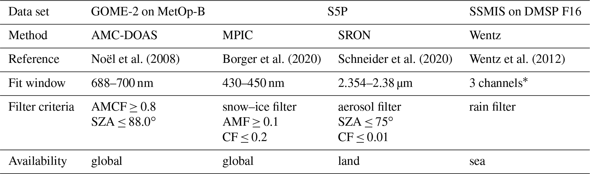
* These channels are 19.35, 22.235 and 37.0 GHz.
2.4.1 GOME-2 AMC-DOAS TCWV
The first GOME-2 instrument on the MetOp series was launched on MetOp-A in October 2006 (Munro et al., 2016). It is an improved version of GOME on the second European Remote Sensing Satellite (ERS-2) (Burrows et al., 1999; Munro et al., 2006). GOME-2 observes the atmosphere in a spectral range from 240 to 790 nm with a spectral resolution of 0.26 to 0.51 nm. By default, its spatial resolution is 80 km across track × 40 km along track with a swath width of 1920 km. Since the launch of MetOp-B in September 2012 both satellites have flown in a tandem operation mode. The swath of GOME-2 on MetOp-A was then reduced to 960 km, resulting in an increase of spatial resolution by a factor of 2 across track at the cost of spatial coverage. MetOp-B has a sun-synchronous descending orbit with an Equator crossing time of 09:30 local time. Since November 2018, MetOp-C has completed the MetOp series.
AMC-DOAS water vapour products are available for all three MetOp sensors (see, for example, Noël et al., 2008), but for the comparisons with S5P data described in the current study the GOME-2 instrument on MetOp-B (version 0.5.5a) has been selected because it provides the best overlap in spatial and temporal coverage. The estimated accuracy of the GOME-2 TCWV depends on cloudiness and TCWV amount and is typically better than 5 kg m−2.
2.4.2 SSMIS TCWV
From 1987, the Special Sensor Microwave Imager/Sounder (SSM/I) flew on satellites of the Defense Meteorological Satellite Program (DMSP). It measures radiances in discrete spectral bands at wavelengths near 1 cm. From 2003 onwards, this series was succeeded by the Special Sensor Microwave Imager and Sounder (SSMIS) on various platforms up to F18 (Kunkee et al., 2008). For comparison studies with S5P presented in the current paper, the dayside data from the SSMIS instrument on the DMSP F16 satellite are chosen. This is because it has an ascending orbit with an Equator crossing time of 15:54, which fits the S5P observation time best.
Its swath width is around 1700 km. SSMIS total water vapour data used here are provided as daily gridded data (0.25∘ resolution) by Remote Sensing Systems (Wentz et al., 2012). SSMIS data are only available over water surface for rain-free situations. The total water vapour product is processed with the algorithm of Wentz (1997) with version v7. The accuracy of the SSMIS TCWV is around 1 kg m−2.
2.4.3 MPIC S5P TCWV
The Satellite Remote Sensing Group at the Max Planck Institute for Chemistry (MPIC) provides a TCWV product from TROPOMI measurements making use of the water vapour absorption in the blue spectral range (Borger et al., 2020). The retrieval consists of the common two-step DOAS approach: in the first step, the spectral analysis is performed for a fit window from 430–450 nm within a linearized scheme. Then, the retrieved slant column densities are converted to vertical columns using an iterative scheme for the water vapour a priori profile shape, which is based on an empirical parameterization of the water vapour scale height. During an extensive theoretical error estimation, the retrieval's TCWV uncertainty has been approximated to about 10 %–20 % for favourable and 20 %–50 % for unfavourable observation conditions. Furthermore, in the framework of a validation study based on daily and hourly measurements, it was demonstrated that the MPIC S5P TCWV product is in very good agreement to reference data sets (e.g. SSMIS) for clear-sky scenarios over ocean as well as over land surfaces. For this study, only measurements have been included for which the effective cloud fraction is between 0 and 0.2, the air mass factor >0.1 and the snow–ice flag indicates snow- and ice-free conditions. The accuracy of the TCWV product is around 25 % (2.8 kg m−2) for TCWV smaller than 20 kg m−2 and around 15 % for TCWV larger than 20 kg m−2.
2.4.4 SRON S5P TCWV
The Netherlands Institute for Space Research (SRON) provides a TCWV product that is restricted to clear-sky scenes over land and separates water vapour isotopes (H2O and HDO) and is retrieved from the SWIR infrared measurements of TROPOMI from 2354 to 2380.5 nm (Schneider et al., 2020). More details about the retrieval approach and settings can be found in, for example, Scheepmaker et al. (2016). The forward model used here ignores scattering, which makes strict filtering of clouds necessary. Cloud filter data from the Visible Infrared Imaging Radiometer on board the Suomi National Polar-orbiting Partnership (Siddans, 2016) are used. The upper threshold for cloud cover is a cloud fraction of 1 %. An additional filter for aerosols is also applied. Values at solar zenith angles larger than 75∘ are discarded. The albedo of water surfaces is too low to retrieve TCWV over oceans, such that only TCWV is used over land surfaces. In this study, we use version 9_1 of this data set, which shows a bias to TCCON stations of 0.06 ± 0.9 kg m−2 (1.1 ± 7.2 %).
2.4.5 ECMWF ERA5 TCWV
The ERA5 reanalysis data set (Hersbach et al., 2020) from the European Centre for Medium-Range Weather Forecasts provides atmospheric parameters such as temperature and humidity computed on 137 levels from surface height to 80 km. It is a model data set in which a large variety of observational data including satellite measurements (e.g. SSMIS), radiosondes and ground stations are assimilated.
This product is available every hour. The data used here are on a 0.25∘ spatial grid. TCWV is derived by vertical integration of the profile data.
3.1 AMC-DOAS approach
The approach known as differential optical absorption spectroscopy was first used to describe active remote-sensing measurements having long tropospheric optical paths. (Perner and Platt, 1979). Variants of DOAS techniques were proposed and have been successfully applied from space (see, for example, Burrows et al., 1999, and references therein) to derive the amount of trace gases in the atmosphere. The method uses the Lambert–Beer law, which describes the attenuation of light due to gas absorption along a light path. The amount of a trace gas along this light path is the slant column density. The slant column density is converted into a total vertical column via a so-called air mass factor. This air mass factor is usually derived from radiative transfer calculations taking the solar geometry and scattering processes in the atmosphere into account.
The standard DOAS approach is in principle only valid for weak absorbers. Water vapour is usually a strong absorber and has a highly structured absorption spectrum, which typically is not resolved by the measuring spectrometer. This results in a non-linearity of the water vapour absorptions, which arises from absorption lines becoming saturated at higher spectral resolution within the spectral line width of the instrument. These have to be accounted for explicitly in the retrieval.
To address this goal, Noël et al. (1999) developed a modified version of the standard DOAS method named air-mass-corrected differential optical absorption spectroscopy (AMC-DOAS). This method uses the equation
where I0,λ and Iλ are the solar irradiance and Earth's backscattered radiance, respectively. The index λ denotes quantities with dependence on the wavelength. is the optical depth of oxygen. The quantity cλ contains the absorption cross section and air mass factor. The exponent bλ accounts for saturation effects in the spectra. As in standard DOAS, P is a low-order polynomial accounting for broadband features such as scattering, liquid water absorption and also variations in the surface albedo. The ring effect is not considered because it is not relevant in our fit window. , bλ and cλ are spectral quantities which are precalculated using a radiative transfer model.
a is the so-called air mass correction factor, which accounts for differences between the real atmospheric conditions and light path compared to those assumed in the radiative transfer calculations. Cv is the total vertical column of water vapour, which is derived together with a and P by a non-linear fit.
This method is applied to the measured Iλ and I0,λ in the spectral range of 688–700 nm, which has been selected because in this spectral region, absorption lines of oxygen and water vapour are both present and of similar strength. This is important because the underlying assumption of AMC-DOAS is that the same correction factor a can be applied to both oxygen and water vapour. This will be explained in more detail in the following.
In the case of a perfect match of model conditions to the true atmospheric conditions, no correction needs to be made. In this case the measured optical depth of oxygen equals the modelled ; thus a=1.0. If there are differences in the light path (e.g. introduced by different meteorological conditions), the oxygen absorption depth differs from that modelled. Hence the correction factor a differs from 1. The factor a scales the spectra such that the modelled oxygen absorption and that measured match one another. We assume that the differences in light path through the atmosphere are the same for the regions of water vapour and oxygen absorption. This approximation enables the scaling factor determined for oxygen spectra to be applied to water vapour.
Up to the present, in studies using TCWV retrieved using the AMC-DOAS method for the GOME-like instruments (Noël et al., 1999, 2004, 2008), a surface elevation of 0 km and a constant surface albedo of 0.05 have been assumed for the determination of the spectral parameters , bλ and cλ via radiative transfer calculations. The parameters are calculated for various solar zenith angles ranging from 0 to 88∘. During the retrieval, the quantities are then interpolated to the actual solar zenith angle of the measurement. A fixed reference H2O profile for a tropical atmosphere with a TCWV of 41.8 kg m−2 from LOWTRAN (Anderson, 1995) is used. No clouds are included in the radiative transfer calculations; thus the retrieval is in general only valid for cloud-free scenes. However, small amounts of clouds can in principle be accounted for by the air mass correction factor a.
The currently existing AMC-DOAS data sets for GOME, SCIAMACHY and GOME-2 use radiative transfer databases, derived from SCIATRAN version 2 (Rozanov et al., 2005) in combination with HITRAN 2004 spectral line data (Rothman et al., 2005). Modelled spectra are convoluted with a Gaussian slit function having an optimized full width at half maximum (FWHM) for each instrument (between 0.35 nm for GOME and 0.59 nm for GOME-2C) to account for the different spectral resolutions. Effects due to different observation geometries are also accounted for by a. Varying viewing angles are therefore not considered within the radiative transfer model.
3.2 Adaption and optimization of AMC-DOAS to Sentinel-5P observations
For the application to S5P reflectance (radiance divided by irradiance) observations, the AMC-DOAS method was adapted in the following way. The radiative transfer model SCIATRAN v3.8 (Rozanov et al., 2014) in combination with the HITRAN 2012 (Rothman et al., 2013) spectral absorption database is used to compute the quantities c, b and . As the reference H2O vertical profile, a tropical atmosphere with a TCWV of 41.8 kg m−2 is used (from the LOWTRAN database). The spectra are then convoluted with the across-track ground-pixel-dependent instrument spectral response functions (ISRFs) (van Hees et al., 2018) of S5P. Their full width half maximum varies around and in the range of 0.34 nm ± 0.002 nm. The spectral quantities are calculated for a reference surface albedo of 0.02, which we assume to be the surface albedo of a water surface in the selected spectral range. The surface height is also accounted for. As the surface height reference, the Global Multi-resolution Terrain Elevation Data 2010 (GMTED2010; Danielson and Gesch, 2011) is used. The radiative transfer database is then calculated for every ground pixel and various surface heights from 0 to 9 km. Note that this added dependence on the surface height also changes the definition of the AMC-DOAS water vapour product. The S5P TCWV is defined as the total column above the surface, whereas in previous AMC-DOAS products, it was defined as the total column above sea level. This has the advantage that TCWV values over mountain ranges are valid data points.
In previous applications for the GOME-like instruments, the scaling factor a was also used as an inherent quality check (Noël et al., 1999). If the correction is too large (which is mainly due to clouds), the retrieval results are discarded. The corresponding minimum air mass correction factor of 0.8 is also used as a filter criterion for the S5P data. However, it turns out that for S5P, this filter is not effective enough. Too many (especially cloudy) data remain. In general, we derive typically higher air mass correction factors for S5P than for the other instruments. We attribute this mainly to the different Equator crossing times (morning vs. noon) in combination with the wider swath width of S5P. Thus, additional filtering is needed to remove unphysical results.
The largest source of error in the AMC-DOAS TCWV product is associated with partially cloud-filled ground scenes. The larger the fraction of cloud within a ground scene and the higher the cloud, then the lower the effective sampling of the troposphere. We therefore apply an additional cloud filter, which is based on cloud fraction and cloud height, provided by the operational S5P FRESCO cloud product. A pixel is considered cloudy if the cloud fraction is larger than 0.2. In addition, measurements with cloud heights above the surface of more than 2.0 km are also discarded.
An example for a S5P-measured spectrum and the corresponding fitted spectrum from the retrieval can be seen in Fig. 1a for a scene over the Pacific with very little cloud fraction. In this example, the retrieved TCWV is 16.0 kg m−2 with an retrieval error of 0.39 kg m−2. The residual, which is given in relative amount (measurement minus fit divided by measurement; see Fig. 1b), is not larger than roughly 0.3 % in this example. The root mean square of the absolute residual (measurement fit) is 0.07, i.e. small. This shows that the measured and fitted spectra match very well.
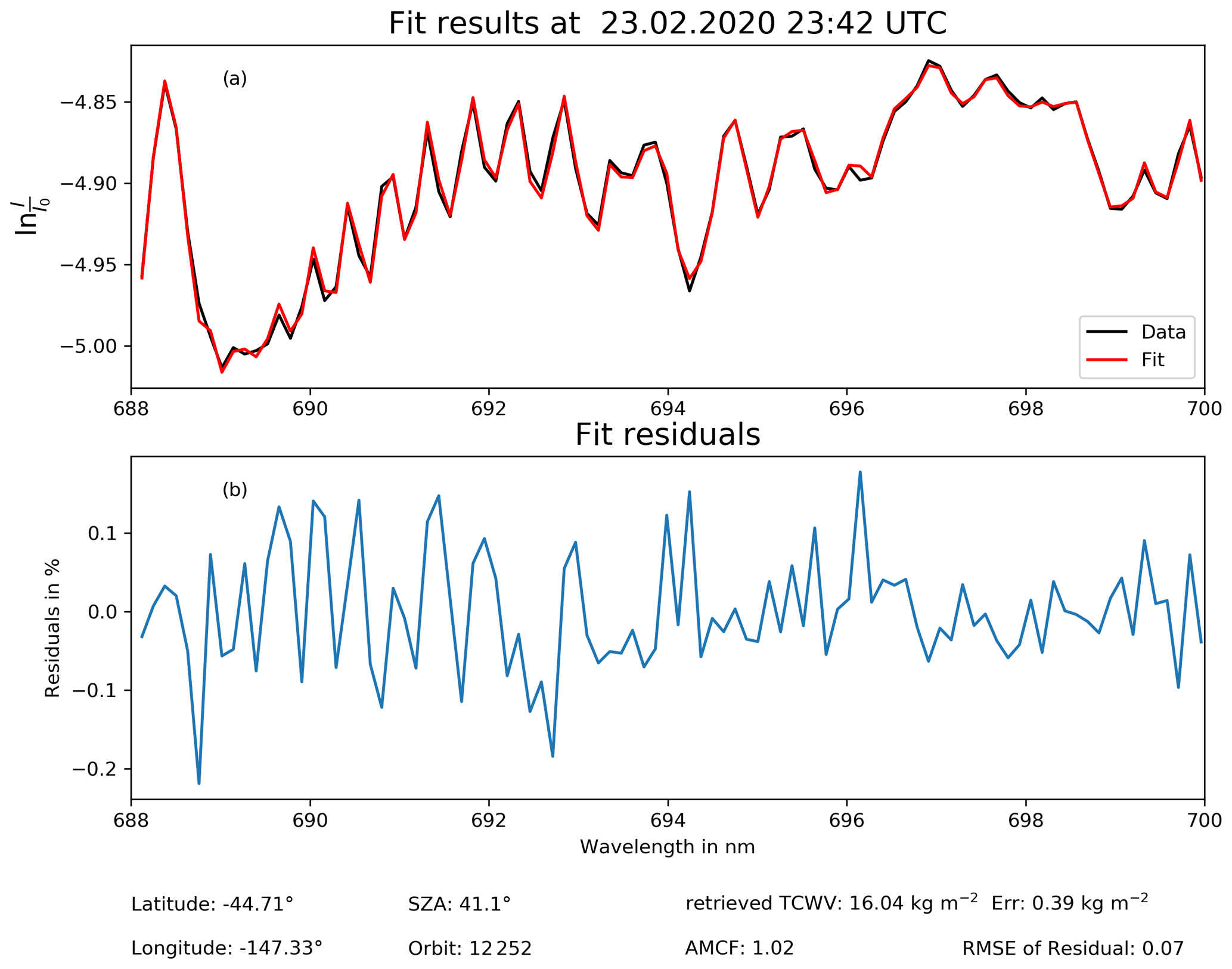
Figure 1(a) Example measurement (black) from S5P and fit (red). (b) Relative fit residual (relative difference between measurement and fit) in percent.
3.3 Post-processing
With the AMC-DOAS method, 1 d of S5P measurements (23 February 2020) has been processed and filtered according to the procedure described above. The resulting S5P TCWV product shown in Fig. 2a represents all expected spatial features. Within the intertropical convergence zone (ITCZ), the values are largest. Towards polar regions, the TCWV decreases.

Figure 2Visualization of the effects of the correction on the AMC-DOAS S5P TCWV on 23 February 2020. Grey areas are data gaps mainly due to the filtering. Panel (a) shows the retrieved AMC-DOAS S5P TCWV with no corrections applied; (c) shows the AMC-DOAS S5P TCWV with albedo and cloud correction as explained in the text; (e) shows the empirically corrected AMC-DOAS S5P TCWV after the cloud and albedo correction. Panels (b), (d) and (e) show the difference of the AMC-DOAS S5P TCWV in (a), (c) and (e) to the ERA5 TCWV (AMC-DOAS S5P TCWV − ERA5 TCWV).
Details on the quality of the AMC-DOAS S5P TCWV are revealed by the deviation to the collocated ERA5 TCWV (Fig. 2b) which shows several issues. For the global average, there is only a small difference of 0.05 kg m−2 between both data sets. Over ocean, repeating patterns of the differences are visible. These patterns are more pronounced over regions with higher TCWV. Over land, systematic positive deviations over regions with higher surface albedo can be observed, such as those observed over Sahara and Australia. These regions typically have a higher surface albedo than the reference used for the AMC-DOAS radiative transfer database. This implies that surface albedo influences on the retrieved AMC-DOAS TCWV need to be considered. Also, remnant clouds will affect the retrieval. Thus an additional correction scheme has been introduced to reduce systematic effects due to variations of surface albedo and clouds. This is described in the following subsections.
3.3.1 Albedo and cloud effects
Clouds hide parts of the atmospheric profile depending on cloud height and cloud fraction. This is especially critical for water vapour, which is most abundant close to the surface. To reduce the impact of clouds, we therefore filter out scenes with cloud fractions larger than 0.2 as a first step.
The effects of varying surface albedo on the measured signal and the light path are in principle handled in the AMC-DOAS method by the fitted polynomial and the air mass correction factor. The remaining influences of albedo on the retrieval results are due to the unequal (and usually unknown) shapes of the water vapour and oxygen profiles. The cloud effect and the albedo effect are not completely separable. It is therefore necessary to derive correction factors for various combinations of cloud fraction, cloud height, surface albedo, surface height and solar zenith angle.
To investigate the dependence of AMC-DOAS TCWV on surface albedo and cloud properties, radiances Iclear and Icloud are simulated with SCIATRAN for the clear-sky case and the fully cloudy case, respectively. Please note that in this paper the term of albedo is used to describe the spectral reflectance from surface and clouds. This assumes a Lambertian surface where the total reflected radiation is homogeneously distributed over a hemisphere, i.e. 2π sr. For the small spectral window used in the retrieval, this is considered a reasonable approach, and spectral dependence of surface albedo is ignored. For the clear-sky case, surface albedo, surface height and solar zenith angle are varied. For the cloudy case, we also consider dependencies on cloud height and cloud fraction.
A cloud is considered in the simulations as a reflecting layer with an albedo of 0.8, which is located at a given height. This follows the definition of the S5P FRESCO product. The simulated cloud-free and cloudy radiances are then mixed by the cloud fraction CF according to the independent pixel approximation:
The spectrum Imixed is then used to retrieve the AMC-DOAS TCWV. The ratio of the reference (“true”) TCWV Cv,ref to the retrieved AMC-DOAS TCWV Cv,retr may then be used as a multiplicative correction factor cac:
Note that the albedo–cloud correction is independent from the retrieval and its parameters. It is applied after the retrieval and uses its own lookup tables. Examples for this correction factor are shown in Fig. 3.
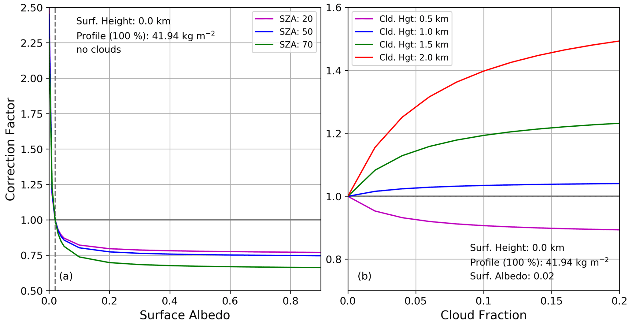
Figure 3(a) Correction factor as a function of surface albedo for various solar zenith angles. (b) Correction factor as a function of cloud fraction for various cloud heights.
If no cloud is present, only the variation of the surface albedo plays a significant role in the AMC-DOAS retrieval (Fig. 3a). In the case of smaller surface albedo than the reference of 0.02, the retrieved TCWV is underestimated; thus the correction factor is larger than 1. Larger surface albedo is associated with an overestimation of the reference TCWV and a correction factor smaller than 1. This is especially true over bright land surfaces such as snow-covered areas and deserts, where the AMC-DOAS TCWV correction would be large. However, after correcting albedo and cloud effects, the AMC-DOAS TCWV no longer depends on the choice of the “default” surface albedo.
An example for the correction factor for cloudy scenes is shown in Fig. 3b. For low-level clouds located at around 500 m above the surface or less, there is an increase of the retrieved TCWV, resulting in correction factors smaller than 1. Low-level clouds hide a relatively small part of the water vapour profile compared to that hidden by higher clouds. As discussed before, albedo leads to an overestimation of total water vapour. Since the albedo of clouds is large, the albedo effect overcompensates for the shielding effect. This effect increases for larger cloud fractions. For clouds higher than 500 m, the shielding effect dominates, resulting in a reduction of the retrieved TCWV and a correction factor larger than 1. It can also be seen that the correction increases for higher clouds and larger cloud fractions.
For the AMC-DOAS TCWV correction, a fixed atmospheric profile is used. The real atmospheric vertical structure of water vapour is highly variable and introduces an uncertainty especially in the AMC-DOAS TCWV cloud correction due to different profile shapes. For example, if there is more water vapour present beneath a cloud than above the cloud layer in comparison to the reference profile, this will lead to an underestimation of the actual TCWV.
To avoid the correction factor dominating the retrieval results, an additional filter is applied to exclude situations where the correction is too large. Thus the correction factor is restricted to values between 0.6 and 1.2.
The final albedo and cloud correction factor depends on geometrical information (solar zenith angle, across-track ground pixel, taken from the S5P measurements), surface elevation (from GMTED2010), cloud fraction and cloud height (from the S5P FRESCO product) and surface albedo.
As the surface albedo is highly variable, we do not use a climatology but determine it directly from the S5P reflectance measurements from 684 to 686 nm. This spectral region is close to the retrieval window of 688–700 nm but contains no major atmospheric trace gas absorption. To relate the reflectance to the surface albedo, radiances and irradiances are simulated from 684 to 686 nm with varying surface albedo, solar zenith angle, surface height, cloud fraction and cloud height. To smooth out fluctuations, the average reflectance over this 2 nm window is calculated. This results in a database from which for each (measured) average reflectance, geometry and cloud properties a surface albedo can be derived via interpolation.
The resulting clear-sky albedo and cloud correction is then applied as a multiplicative factor (cac) to obtain the corrected TCWV:
where Cv,uc is the uncorrected TCWV. Note that due to this correction, the TCWV product is independent of the surface albedo chosen as reference for the basic AMC-DOAS retrieval.
The results of this correction when applied to the uncorrected data from 23 February 2020 are shown in Fig. 2c and their differences to the values in ERA5 in Fig. 2d. The global mean deviation is slightly increasing, but the variability denoted by the standard deviation (SD) is lower compared to the uncorrected product. Over land, the application of the correction factors reduces the differences over the deserts. However, over ocean there are still some patterns visible. These stripe-like deviations resemble orbital features. In the eastern part of the S5P swath, the TCWV is generally lower than ERA5 TCWV. It has to be noted that over ocean where the surface albedo is very low, the signal may be dominated by residual clouds. If the cloud fraction is too high (low), the retrieved surface albedo is too low (high). This also affects the correction factors, which means that the AMC-DOAS TCWV product quality depends on the accuracy of the cloud product. Because of different conditions over land than over sea (higher surface albedo, different aerosol types), using the same filtering limits may in principle lead to a systematic land–sea bias. However, since the chosen limits are quite wide, this effect is small. For example, the cloud and albedo correction filter removes only less than 1 % of the data.
3.4 Empirical correction for the across-track features
The stripe-like deviations over ocean shown in Fig. 2d cannot be reproduced by our clear-sky model. The reason for this effect is not clear. It could be an instrumental effect due to stray light, which may have a larger effect over ocean than over land because of the lower ocean albedo. However, other effects not explicitly included in our model, such as aerosols, glitter/glint and non-Lambertian surface reflectance, may also play a role. In fact, the across-track features are similar to the observation of Grossi et al. (2015), who could attribute this to non-Lambertian surface effects. To eliminate this repeating pattern, an empirical correction is performed. This correction only depends on the relative location of the across-track ground pixel. We investigated the temporal behaviour of the empirical correction. The general shape was similar for all months, so we decided not to include any temporal dependence. We also do not see a large dependence on solar zenith angle. Note that varying viewing geometry is already accounted for by the air mass factor correction, so this already removes many dependencies. The albedo correction handles further parts of the across-track features (e.g. sun glint is removed). Since the across-track features are only visible over ocean and not over land, the correction will only be applied to across-track ground pixels located over water surfaces.
For this purpose, for each swath over the water surface, the relative difference ΔCv,ac of the retrieved TCWV at each across-track ground pixel i to the nadir value (across-track ground pixel inadir=223) is computed:
All S5P orbits in February 2020 are used for this to obtain good statistics. For every across-track ground pixel with valid TCWV measurement, ΔCv,ac(i) is calculated and counted with bins of 0.05. This results in a histogram of ΔCv,ac as a function of the across-track ground pixel number, which is shown in Fig. 4. As can be seen, there is a systematic across-track ground pixel dependence of ΔCv,ac. In the western part of the swath (across-track ground pixel numbers smaller than inadir), the relative difference is positive, whereas the eastern part (across-track ground pixel numbers larger than inadir) shows more pronounced negative differences.
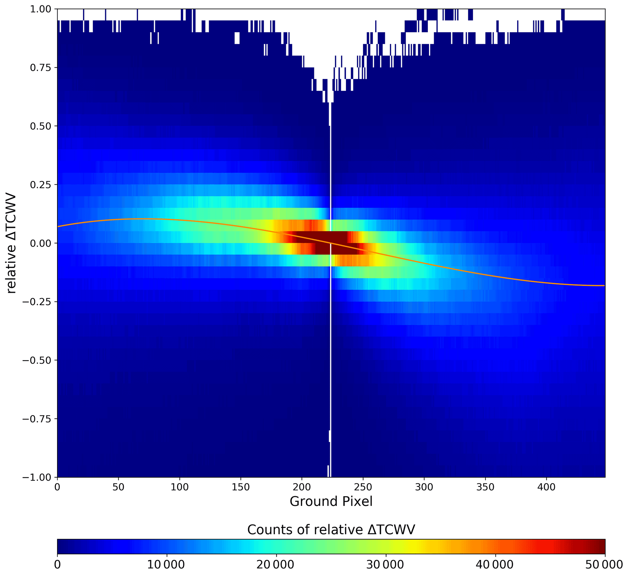
Figure 4The number of measurements, i.e. counts of the relative difference between the albedo and cloud-corrected S5P TCWV to the nadir value for every ground pixel for February 2020. The orange line is a third-degree fitted polynomial.
For the correction, the maximum amount of ΔCv,ac at each across-track ground pixel is then used to fit a third-degree polynomial Pemp (orange line in Fig. 4):
where is the shifted across-track ground pixel number, and aj denotes the derived polynomial coefficients, namely: a0=0.0, , and .
The multiplicative correction factor cemp for every across-track ground pixel is then defined as
This correction is then applied in addition to the cloud and albedo correction, leading to
The results are shown in Fig. 2e and f. The spatial patterns over ocean are corrected out, and the mean deviation to ERA5 and the scatter of the data are also reduced.
Note that all applied corrections do not significantly change the water vapour patterns (Fig. 2a, c, e) but generally result in a smoother spatial distribution.
All S5P radiances from May 2018 to December 2020 were processed by the AMC-DOAS method and corrected as described above. The typical precision of the AMC-DOAS S5P TCWV for a single measurements (derived from the fit) is about 0.5 kg m−2.
From these, a daily gridded data product with a spatial resolution of 0.25∘ × 0.25∘ is produced, resulting in a data set called TCWVAMC,S5P in the following. An overview of this TCWV product is given in Fig. 5, which shows the spatial distribution of TCWVAMC,S5P for 4 months.
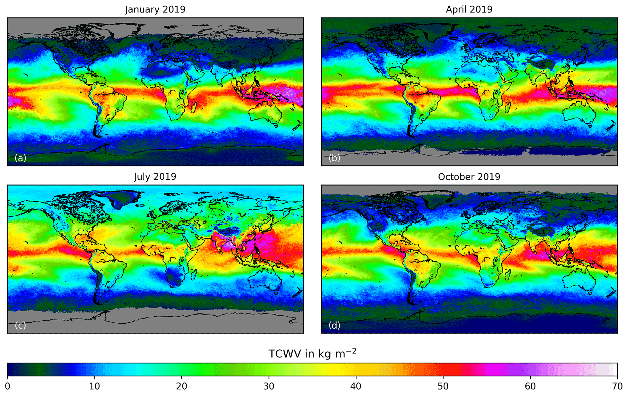
Figure 5Global maps of mean TCWVAMC,S5P for 4 months in 2019.
The general features shown in the maps meet the expectations from climatology. In the tropics, there is higher TCWV due to high temperature. Within the ITCZ, the values are highest. Towards the polar regions, the air becomes colder; thus the TCWV decreases. The propagation of the main features during the course of the time is also visible. The global average of TCWV is around 18.5 kg m−2.
In January, the ITCZ is located close to the Equator. During the course of time, it shifts northwards until July. Large changes are observed comparing January and July over southeast Asia (e.g. India, China) and nearby water surfaces. Here the ITCZ reaches its northernmost position, causing an increase of TCWVAMC.S5P of around 30 kg m−2 from January to July.
During northern summer as the entire Northern Hemisphere warms, the global average TCWV is largest (23.1 kg m−2). This is in large part due to larger land masses in the Northern Hemisphere. They are significantly warmer during July than the large oceans in the Southern Hemisphere in January. Smaller contributions come from Arctic regions, which also show enhanced TCWV. Such a large TCWV increase cannot be observed from July to January over the Southern Hemisphere due to the lack of land masses.
TCWVAMC,S5P also shows some differences between April and October. In general, all features follow the position of the sun but with a time lag of several weeks. That means in April the Northern Hemisphere is colder, which results in higher TCWV in October.
Over sea the averaged TCWVAMC,S5P is higher than over land due to different surface elevation, larger temperature variability and also the evaporation over water surfaces. No data are available in the winter hemisphere's polar night region due to a lack of solar insolation.
To assess the quality of this new data set, it is compared to various other data sets (see Sect. 2.4 for more information), which are either also provided on a daily 0.25∘ × 0.25∘ grid or have been gridded accordingly. We use the following notation for these correlative data sets:
-
TCWVAMC,GOME-2B. The GOME-2B data product is based on the original AMC-DOAS approach and is daily gridded to 0.25∘ × 0.25∘.
-
TCWVWENTZ,SSMIS. The SSMIS data product uses microwave emissions as input and is provided on a daily 0.25∘ grid.
-
TCWVMOD,ERA5. ECMWF ERA5 model data are provided every hour on a 0.25∘ grid. Based on the position of every S5P pixel, the spatial and temporal nearest ERA5 TCWV is chosen. This results in a pseudo swath data set consisting of ECMWF data at geolocations of S5P, which is filtered according to the AMC-DOAS filter criteria. These pseudo swaths are then daily gridded to 0.25∘ × 0.25∘ resolution.
-
TCWVMPIC,S5P. The S5P TCWV product data from MPIC in Mainz use the “blue” spectral range, provided on a daily 0.25∘ grid.
-
TCWVSRON,S5P. The S5P TCWV product data from SRON use the SWIR spectral range and are daily gridded to 0.25∘ × 0.25∘.
In the first step, daily TCWVAMC,S5P data are compared to other daily TCWV products. Global deviation maps are then presented and discussed. The comparisons are done over land and ocean separately to detect possible systematic features arising from surface type and/or elevation. It has to be noted that all satellites have different overpass times; thus diurnal changes in TCWV may affect the comparison results.
4.1 Daily comparisons
The comparison procedure for the daily data is as follows. For every day, TCWVAMC,S5P and the other TCWV products are collocated. From the collocated data sets, pairwise differences ΔTCWVAMC,S5P-Z are calculated:
Here, the index Z denotes the specific data set used for comparison. Additionally, the difference is averaged by weighting according to the cosine of the latitude, and its variability is given by the standard deviation (SD).
A linear regression model using a least-squares technique is applied to TCWVAMC,S5P and TCWVZ. This gives the correlation coefficient R and the regression parameters n and m, denoting the intercept and the slope, respectively.
A scatter plot for 23 February 2020 is shown in Fig. 6 for the various TCWV products. All statistical parameters are given in Table 2.
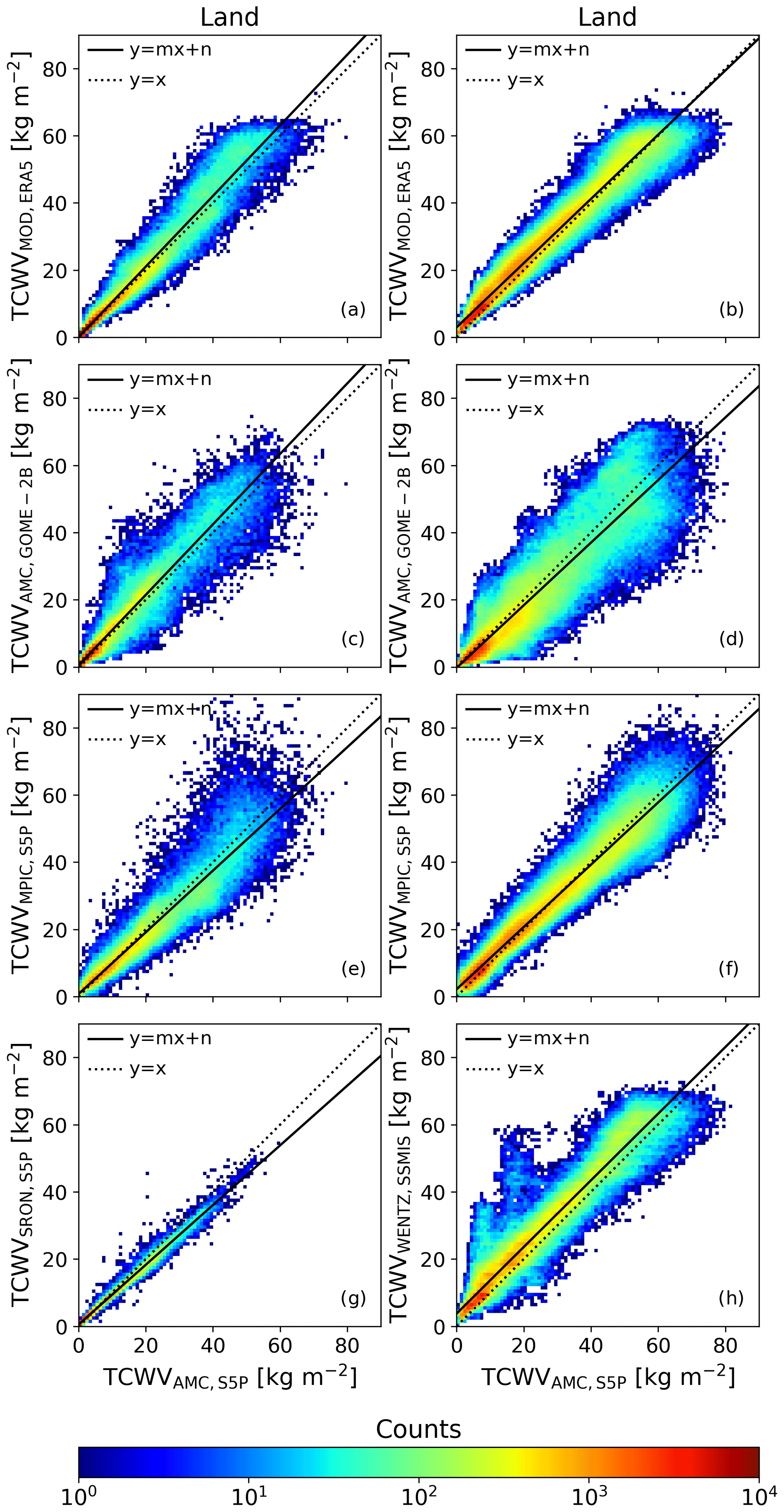
Figure 6Density plots of TCWV comparisons with the AMC-DOAS S5P product over land (a, c, e, g) and over sea (b, d, f, h) for 23 February 2020 for (a) and (b) ERA5 TCWV, (c) and (d) AMC-DOAS GOME-2B TCWV, (e) and (f) MPIC S5P TCWV, (g) SRON S5P TCWV and (h) SSMIS TCWV. The dotted line represents perfect agreement (1:1), and the solid line shows the (fitted) linear relationship between the data sets. All statistical parameters are given in Table 2.
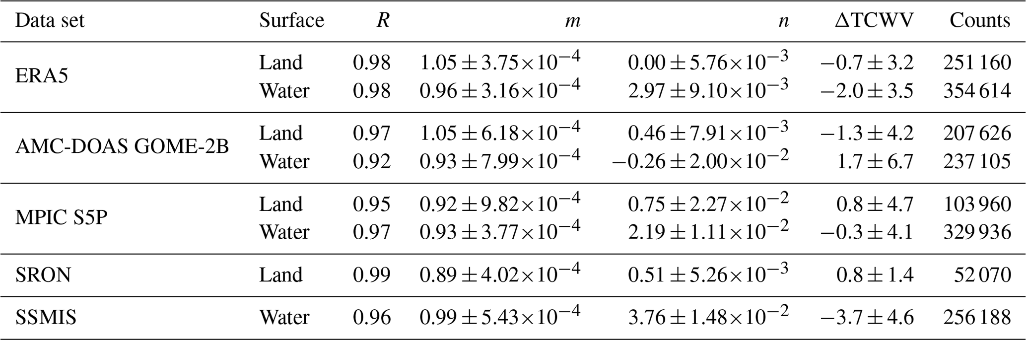
Table 2Pearson correlation coefficient R, slope m, intercept n, average difference ΔTCWV (in kg m−2) to the AMC-DOAS S5P product and collocation counts for the scatter plots in Fig. 6. The errors represent 1 standard deviation.
4.1.1 ERA5
ERA5 is a model compromising satellite data (e.g. SSMIS), radiosondes and weather observations for reanalysis. That makes TCWVMOD,ERA5 a very robust TCWV product. Due to the fact that ERA5 is an hourly data set, temporal mismatch is restricted to less than half an hour.
The comparison between TCWVAMC,S5P and TCWVMOD,ERA5 (Fig. 6a, b) shows a very small difference of −0.7 kg m−2 (Fig. 6a) over land. The values are orientated along the 1:1 line, which is also denoted by the small standard deviation of 3.2 kg m−2. Over sea (Fig. 6b) the difference is larger (−2.0 kg m−2) than over land, but the standard deviation (3.5 kg m−2) and also the correlation coefficient are very similar. The correlation coefficients are above 0.98, indicating a very good agreement between both data sets.
4.1.2 GOME-2B
The comparison between TCWVAMC,S5P and TCWVAMC,GOME-2B (Fig. 6c, d) shows very good agreement between both data sets, irrespective of whether the retrieved TCWV is over land or water surfaces. This is demonstrated by the regression line (solid line in Fig. 6c, d) being very close to the 1:1 line (dotted) and a correlation coefficient above 0.9.
The average TCWV difference ΔTCWVAMC,S5P-AMC,GOME-2B is −1.3 ± 4.2 kg m−2 over land (Fig. 6c), i.e. close to zero (see Table 2 for further details). Because the slope of the regression line is nearly 1, there is only little dependence of the difference on the magnitude of the TCWV. Due to the large number of lower TCWV around 10 kg m−2, the linear regression model is more weighted to these values. Over ocean (Fig. 6d), there is more variability in the difference, which is also indicated by the standard deviation of 6.7 kg m−2. The average deviation is 1.7 kg m−2. There is a land–sea bias of 3 kg m−2 on this day.
Both products are processed with AMC-DOAS. In contrast to TCWVAMC,GOME-2B the surface height is considered during the retrieval of TCWVAMC,S5P, which explains higher values of TCWVAMC,GOME-2B over land. The additional post-processing only done for TCWVAMC,S5P also affects the results.
Other sources that influences the comparison results are the filters applied to the TCWVAMC,S5P. As mentioned above TCWVAMC,S5P data are filtered with an additional cloud filter, which is not applied to GOME-2B data. The propagation of large-scale cloud decks such as in lows or the well known stratocumulus cloud region is not that fast within the time difference of MetOp-B and S5P overpasses of 4 h (at Equator). These cloud decks are therefore located at similar positions for both overpass times. Thus cloud masking applied to TCWVAMC,S5P will also filter clouds by some degree from TCWVAMC,GOME-2B (as we only consider grid points where both instruments have data).
4.1.3 MPIC S5P
The TCWVAMC,S5P and TCWVMPIC,S5P both use S5P Level 1 measurements, but different spectral regions are used in the retrieval. Over land (Fig. 6e), the mean difference between both data sets is 0.8 kg m−2, with a standard deviation of 4.7 kg m−2. The TCWVMPIC,S5P data contain a few values up to 90 kg m−2, which are not observed in the TCWVAMC,S5P. Over land, there are fewer valid data in TCWVMPIC,S5P compared to other data sets, which can be seen from the number of valid counts (Table 2) after collocation. This is due to the filtering of snow- and ice-contaminated scenes.
Over sea (Fig. 6f), there is almost no mean deviation (−0.3 kg m−2) and a lower variability (4.1 kg m−2) than over land. The differences are smallest over both land and sea compared to the other data sets. This meets the expectations because measurements are performed by the same instrument. Nevertheless, uncertainties may arise from sampling differences.
4.1.4 SRON S5P
The TCWVAMC,S5P and TCWVSRON,S5P also use the data from the same instrument. In contrast to TCWVMPIC,S5P, the SRON product has a poorer spatial coverage due strict cloud filtering and limitation to land. The main aim of the SRON data product is to provide columns with low error caused by cloud contamination. This results in 50 000 collocated grid points over land (see Table 2) being available for comparison. Figure 6g also illustrates this. There is far less scatter visible than for the other data sets. Most of the TCWV pairs are well oriented along the regression line. This is also shown by an almost perfect correlation coefficient of 0.99. On average, the difference between TCWVAMC,S5P and TCWVSRON,S5P is 0.8 kg m−2. The standard deviation is 1.4 kg m−2, which is comparably low with respect to the other TCWV products; the TCWVSRON,S5P rarely exceeds 40 kg m−2. Both low scatter and low total columns are probably related to the filtering, which removes almost all even partly cloudy scenes, i.e. especially those scenes which require dedicated corrections in the other S5P TCWV algorithms.
4.1.5 SSMIS
Microwave instruments are known to provide good information on total water vapour because microwave emission penetrates through clouds. However, the comparison to TCWVAMC,S5P is limited to ocean areas because SSMIS does not provided data over land surfaces.
The mean deviation between TCWVAMC,S5P and TCWVWENTZ,SSMIS is the largest compared to other data sets (−3.7 kg m−2). The regression line in Fig. 6h shows a constant offset between both data sets. There are several possible reasons to explain this large offset:
-
The DMSP F16 has an orbit later in the afternoon (around 16:00 LT). This can affect the TCWV due to slight warming of the sea surface and the above air. This causes enhanced evaporation and thus a slightly higher water vapour content.
-
In the microwave region, the radiation penetrates through the clouds. As a consequence, SSMIS senses the entire profile if clouds are also present. The total water vapour is usually higher in cloudy scenes than in clear-sky scenes, which is also referred to as the clear-sky bias (Gaffen and Elliott, 1993; Sohn and Bennartz, 2008). In TCWVAMC,S5P, data with cloud fractions above 0.2 are excluded, which introduces a negative offset.
-
The AMC-DOAS retrieval and also the cloud and albedo correction for S5P use a tropical profile as a reference. Usually the reference profile shape and the true profile shape differ. That also can cause systematic differences, especially in the presence of residual clouds.
-
The cloud and albedo treatment is dependent on the quality of the cloud products used. Uncertainties in the cloud product will have an impact on the surface albedo estimation and also on the calculation of the correction factors.
There also are some values where TCWVWENTZ,SSMIS exceeds TCWVAMC,S5P by more than 20 kg m−2. These arise from two DMSP F16 orbits located between the International Date Line and North and South America. Those orbits belong to the very first orbits of the daily SSMIS TCWV product. For the TCWVAMC,S5P, the transition between the first and last orbit of the specific day is located much closer to the International Date Line. This results in a time mismatch of roughly 24 h between S5P data and SSMIS data in these areas, causing these observed TCWV differences.
4.2 Time series of TCWV differences
Since TCWVAMC,S5P is available for more than 2 years, it is worthwhile investigating the behaviour of differences of TCWV through time. Figure 7 shows the daily averaged TCWV differences between the TCWVAMC,S5P product and the different correlative data sets from May 2018 to December 2020. Again, this is done for the land surface (Fig. 7a) and water surface (Fig. 7c) separately. The respective standard deviations are also shown (Fig. 7b, d).

Figure 7Time series of the daily averaged difference between TCWVAMC,S5P and TCWV from other data sets over land (a) and water (c) surface from May 2018 to December 2020. The right panels show the respective standard deviation over land (b) and water (d).
The temporal behaviour of the TCWV difference between the AMC-DOAS products for S5P and GOME-2B over land shows a systematic deviation between −1 and −2.5 kg m−2; also, a seasonal cycle is visible. The largest deviations can be seen during the northern summer months, whereas in northern winter the deviation is lowest. The standard deviation also shows a seasonal cycle, with largest variability also during northern summer. Compared to the other data sets, the average difference is largest.
The behaviour of the difference to the AMC-DOAS S5P product is quite different for the S5P data set from MPIC. There is a clear jump of around 1.8 kg m−2 located on 20 March 2019. This is due to an update of the TROPOMI FRESCO-S cloud product used in the generation of TCWVMPIC,S5P, which affects the retrieved TCWV. FRESCO-S is a specific cloud product based on the FRESCO algorithm but adapted to the retrieval of NO2. It differs from the FRESCO cloud product used for the AMC-DOAS, for example, in the spatial resolution. Before the jump the difference is between 0.5 and −1 kg m−2; thereafter the difference is slightly positive. This jump mainly originates from the tropical regions where evergreen rainforests are common, for example, the Amazon rainforest.
The differences also shows a seasonal cycle, which is of opposite sign, compared to the difference between the two AMC-DOAS data sets. The seasonal cycle cannot be observed in the standard deviation. The standard deviation of ΔTCWVAMC,S5P-MPIC,S5P reveals a reduction of about 1 kg m−2 caused by the effects of the change in the FRESCO-S cloud product.
The difference between TCWVAMC,S5P and TCWVSRON,S5P shows a deviation of around 1.2 kg m−2 and also a seasonal cycle with least differences in northern winter and largest differences during northern summer. This is similar to the seasonality of ΔTCWVAMC,S5P-MPIC,S5P. After March 2019, the deviation to both S5P TCWV products is also very similar. On 7 March 2020, there was a change in the cloud product used by SRON. As for ΔTCWVAMC,S5P-MPIC,S5P, this causes a small jump in ΔTCWVAMC,S5P-SRON,S5P of around 0.5 kg m−2. The standard deviation varies around 1.5 kg m−2, which is lower compared to other TCWV products. The TCWVSRON,S5P is filtered with a very strict cloud filter that only left small TCWV values. Therefore TCWV values from tropical regions where TCWV is high are discarded.
Between TCWVAMC,S5P and TCWVMOD,ERA5, there is a general negative deviation around 1.6 kg m−2. In contrast to the other data sets, only very small seasonal variability can be seen.
In summary, the mean difference between TCWVAMC,S5P and other TCWV data varies in the ranges from −1 to −4 kg m−2. The smallest difference is observed between TCWVAMC,S5P and TCWVMPIC,S5P. The difference of TCWVWENTZ,SSMIS to TCWVAMC,S5P, which varies in the range from −3 to −4 kg m−2, is consistently the largest throughout the period of measurement. With the exception of the difference between the two AMC-DOAS products, there is also a small seasonal feature in ΔTCWV, the largest differences being between TCWVAMC,S5P and other data products in January and smallest in July. The differences for different seasons are also of similar magnitude. In contrast to land and also to other data sets over ocean, the mean difference between TCWVAMC,S5P and TCWVAMC,GOME-2B is positive without seasonal features. The standard deviation of the TCWV differences ranges between 3 and 5 kg m−2, with the exception of ΔTCWVAMC,S5P-AMC,GOME-2B, which is around 6 to 7 kg m−2.
At the end of November 2020, there was a version change in the FRESCO product, which is used to correct for cloud effects and is also used to calculate surface albedo to derive the AMC-DOAS S5P TCWV product. This caused a general increase of 2.3 kg m−2 in TCWVAMC,S5P over both land and water surfaces. Due to this increase, the differences show this jump of around 2 kg m−2, except for ΔTCWVAMC,S5P-MPIC,S5P.
4.3 Assessment of the spatial dependence of the difference
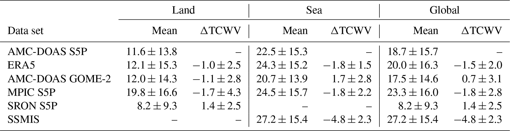
To investigate possible reasons for, for example, the seasonal cycle or the different temporal behaviour among the data sets, we present monthly mean global maps of all data and their difference to our new product. The monthly comparison is restricted to January and July 2019 because all typical spatial and temporal features are already seen from these months. Values for the global average of the TCWV products and its standard deviation and also their difference to TCWVAMC,S5P can be found in Table 3 for January and Table 4 for July.
Table 3Global average (± standard deviation) of the TCWV products and average difference to the AMC-DOAS S5P TCWV product (ΔTCWV) for January 2019 in kilograms per square metre (kg m−2).
4.3.1 ERA5
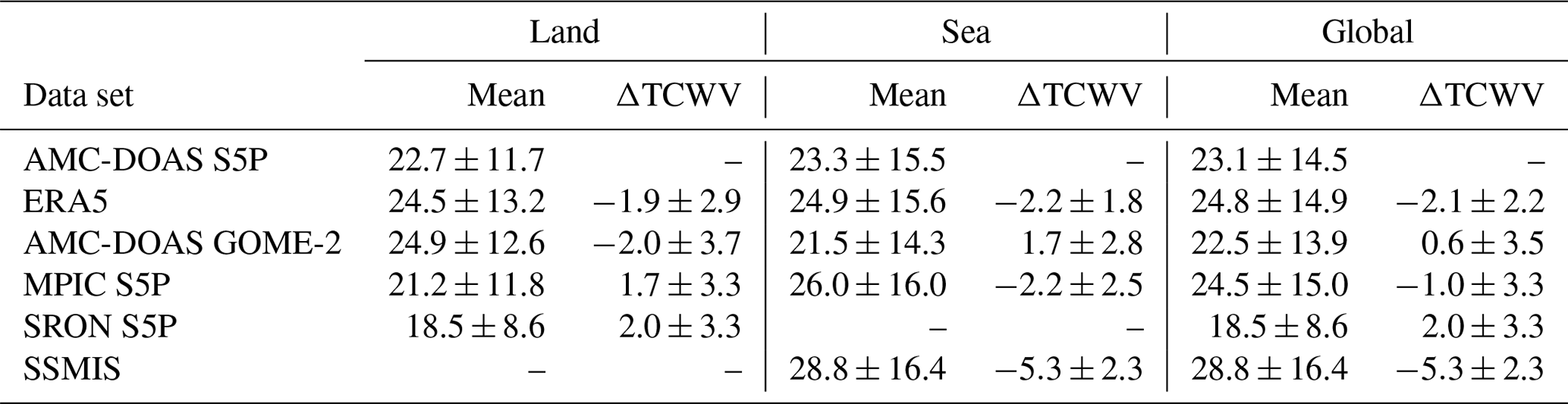
Figure 8 shows a comparison of the AMC-DOAS S5P TCWV products with ERA5 model data. The temporal and spatial sampling of the ERA5 data is the same as for TCWVAMC,S5P because we selected the closest model data point for each S5P measurement. All spatial features of the differences can be seen in Fig. 8b and d.
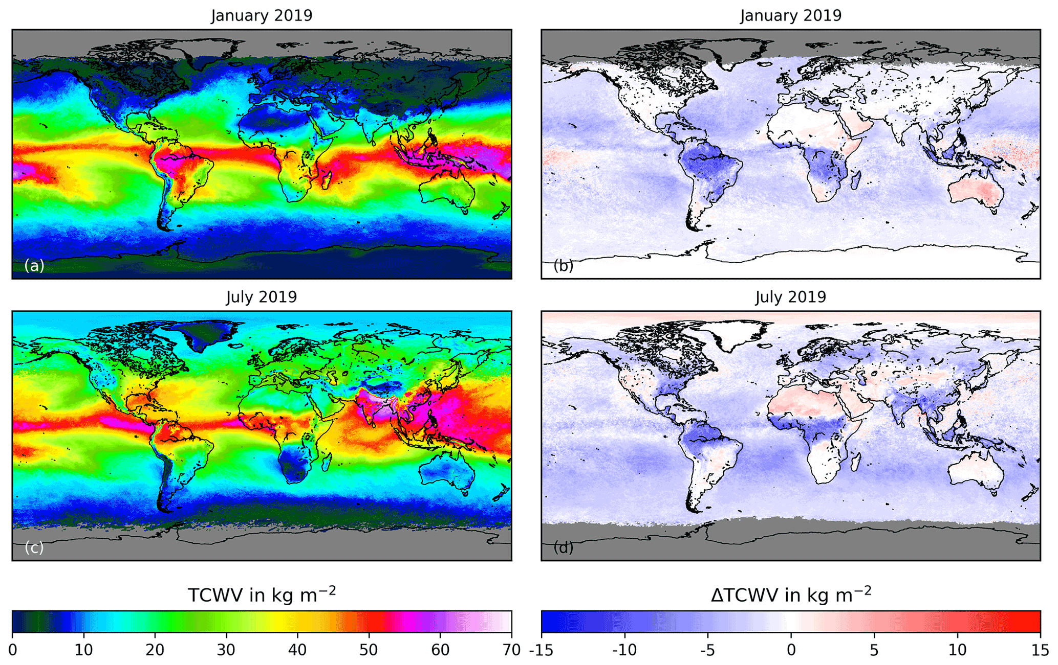
Figure 8Global map of monthly averaged ERA5 TCWV (a, c) and the difference AMC-DOAS S5P TCWV − ERA5 TCWV (b, d) for January and July 2019 (a–d).
Overall, the ERA5 TCWV is slightly larger than the AMC-DOAS S5P TCWV. On global average, the deviation varies around −1.5 kg m−2, with a standard deviation of 2.0 kg m−2 for January. In July, there is a larger deviation of −2.1 kg m−2 and also a larger standard deviation of 2.2 kg m−2, which originates from features over land. Over land, the deviation is around −1.0 kg m−2, with a variability not larger than 2.5 kg m−2. The tropical region contributes most to the negative deviation in all time periods. In July, the negative deviation spreads northward. The large tropical differences are collocated with the evergreen rain forests in the Amazon region, central Africa and also the tropical islands of Asia. July is a season of vegetation growth in the Northern Hemisphere; i.e. the leaves on the trees grow. This pattern reveals potential influences of vegetation either on the TCWVAMC,S5P or on the FRESCO product, which is used as input for the correction. Other features are also seen in large parts of central Australia in January and Sahara in July. Both regions are deserts; they show positive deviations up to 5 kg m−2 during local summer months. In spite of both features the differences between TCWVAMC,S5P and TCWVMOD,ERA5 over land are very close to zero over large regions. The observed negative differences between ERA5 TCWV and AMC-DOAS S5P TCWV at tropical regions, for example, tropical rain forests, correlate with regions of low data availability. We infer that these values are possibly less reliable.
Over sea the differences, which range from −1.8 to −2.2 kg m−2, are larger than over land by 0.3 kg m−2 in July and around 0.8 kg m−2 during January. The distribution of the difference is homogeneous, which is consistent with the reduced standard deviation of around 1.5 kg m−2. Within the 30∘ S and Equator band the differences are slightly larger than in other regions in July.
4.3.2 GOME-2B
In general, the monthly averaged TCWVAMC,GOME-2B (Fig. 9a, c) shows the same features as TCWVAMC,S5P (Fig. 5). The main differences to TCWVAMC,S5P are evident over the tropics where TCWVAMC,GOME-2B barely exceeds 50 kg m−2. There are no TCWVAMC,GOME-2B data over Himalayan mountain ranges due to exclusion of GOME-2 values when the air mass correction is too large.
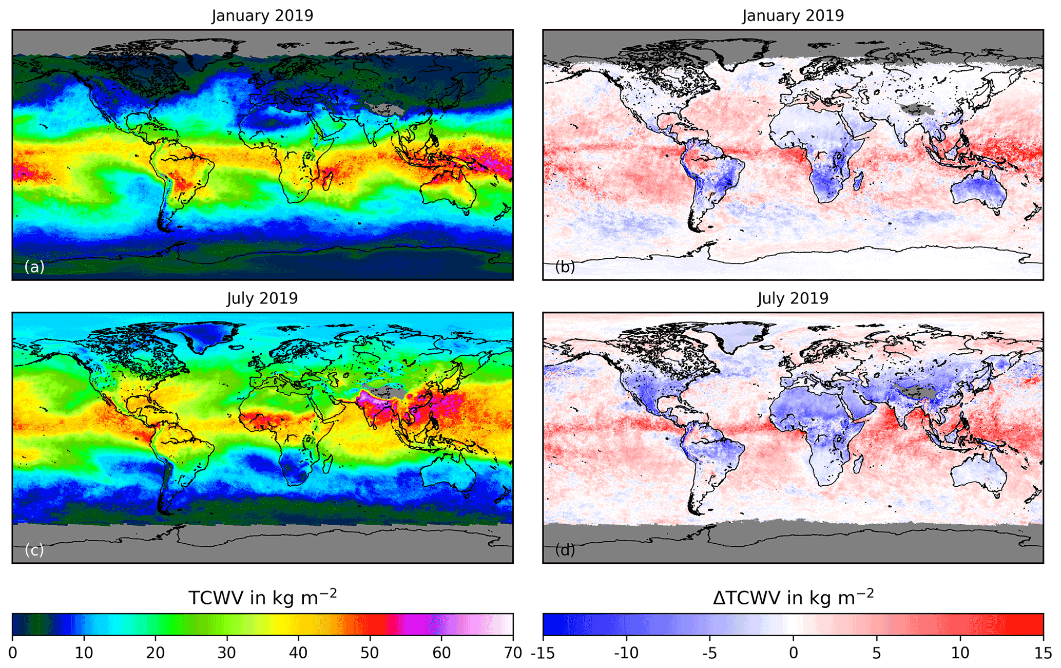
Figure 9As Fig. 8 but for the AMC-DOAS GOME-2B TCWV product.
More details are revealed in the difference maps (Fig. 9b, d). As can be seen, there are systematic spatial structures in the differences. In general, the highest differences both over land and water occur close to the tropics where absolute TCWV is high. In the mid-latitudes and polar regions, the deviations are close to zero. Over land surfaces, negative differences occur often, for example, over the whole of Africa or India. In particular, over Africa several effects can be seen. In the northern part where the surface is bright due to the deserts, the albedo correction reduces the TCWVAMC,S5P, resulting in a difference of around −5 kg m−2, especially in July. The southeastern part of Africa also shows enhanced differences. This region is typically more elevated than the northeastern part. This difference in the surface elevation is only considered in the TCWVAMC,S5P product, which results in lower TCWV over mountain regions and thus explains the larger retrieved TCWVAMC,GOME-2B (which represents the column from sea level) there. These differences are therefore mainly due to the definition differences between both data sets. In July the deviations over land are largest and widely spread throughout the Northern Hemisphere due to an overall increase of TCWV.
Over sea, the difference is overall positive. Since over ocean the surface height is zero, the differences between the two data products cannot be attributed to the different TCWV definitions; they have to be related to the post-processing, which is only performed for the S5P product. The mean sea surface albedo does not differ much in the assumptions made in the retrievals; therefore differences caused by the post-processing corrections are more likely to be related to clouds.
The largest differences are observed in the tropical area where the average TCWV is largest. The ITCZ, where highest TCWV occurs, is also often covered by clouds due to enhanced convection. Here, the correction of cloud effects affects the already high TCWV in the tropics more than in other regions.
The difference of the crossing time of GOME-2 on MetOp-B and Sentinel-5P at the Equator is about 4 h. This also can have an effect due to diurnal cycles in TCWV and in cloud cover. In some areas, for example, the stratocumulus cloud shields over ocean, there is a diurnal cycle with enhanced cloud cover in the morning hours and decreased cloud cover during the afternoon hours (Noel et al., 2018). This may reduce the retrieved TCWVAMC,GOME-2B due to more clouds appearing during the morning overpass of GOME-2 on MetOp-B. Over land, the situation is reversed due to more pronounced convective clouds in the afternoon hours.
The daily comparison between TCWVAMC,S5P and TCWVAMC,GOME-2B discussed earlier showed a quite large standard deviation of about 6 to 7 kg m−2. We infer that this behaviour is related to the spatial structure of the differences over the sea surface where the largest differences are found in the tropics.
4.3.3 MPIC S5P
The S5P TCWV data sets provided by MPIC provide the opportunity to compare different methods applied to the same instrument. This reduces the effect of possible temporal changes of TCWV as a source of uncertainty in the comparison results. The averaged TCWVMPIC,S5P (Fig. 10a, c) shows similar structures as TCWVAMC,S5P (see Fig. 5 for comparison). Over the western Pacific close to Indonesia, there are values up to 70 kg m−2, which are not found in the averaged TCWVAMC,S5P.

Figure 10As Fig. 8 but for the S5P TCWV product from MPIC.
Significant differences between TCWVAMC,S5P and TCWVMPIC,S5P (Fig. 10b, d) occur over land in tropical regions (Amazonas, Indonesia, central Africa) during January. As mentioned before, there was a jump in the daily averaged difference between both data sets at 20 March 2019 due to changes in cloud parameters used by MPIC. Before this change, ΔTCWVAMC,S5P-MPIC,S5P is enhanced in these regions (see Fig. 10b). In July (Fig. 10d), ΔTCWVAMC,S5P-MPIC,S5P no longer shows such large values as in January.
In other areas, the differences are much smaller. Australia shows larger positive differences during January, but also in South America and in southern parts of Africa, positive differences are observed. During July, all land masses on the Northern Hemisphere show constant positive differences, whereas south of the Equator, there are negligible differences.
Over sea, there is an overall negative difference, which is slightly larger in July (−2.2 kg m−2) than in January with −1.8 kg m−2. Large areas of negative differences are observed in the Southern Hemisphere during July, whereas in the Northern Hemisphere the differences are very close to zero. A reversed pattern is slightly visible in January. In this case the largest differences are seen close to Indonesia. The ITCZ is also marked by the narrow band of slightly negative difference. We attribute this behaviour to arise from the use of different cloud correction schemes.
4.3.4 SRON S5P
Figure 11a and c show the TCWVSRON,S5P. The data gaps within the tropics are clearly visible. Despite monthly averages, there are no data within 1 month there. We infer that this is related to the strict cloud filtering. The tropics are associated with the highest cloud occurrence.
Figure 11As Fig. 8 but for the S5P TCWV product from SRON.
The difference to the monthly averaged AMC-DOAS S5P data (ΔTCWVAMC,S5P-SRON,S5P) is mainly positive during January (Fig. 11b). On average, the difference is 1.4 kg m−2 for this month. Southern Hemisphere land masses except for the Antarctic show quite large positive differences up to more than 10 kg m−2 during January. The largest differences are observed in the northern part of Australia. The Northern Hemisphere shows only small and spatially homogeneous positive differences during January.
In July, the land masses on the Southern Hemisphere are associated with positive differences over South America, whereas over Australia and southern Africa, the difference between both S5P TCWV products is very close to zero. Some locations or spots with large positive differences are found in parts of the United States, northern India and also parts of China. These areas suffer from poor data availability of TCWVSRON,S5P, such that the average comprises a few days of measurements. The averaged difference is slightly larger in July with 2.0 kg m−2.
Note that in many cases, the TCWVSRON,S5P monthly averages consist of not more than 5 d or less. Actually, only over deserts are daily data available for more than half of the month. This sampling difference between the products may explain some of the observed differences.
4.3.5 SSMIS
The spatial distribution of TCWVWENTZ,SSMIS is shown in Fig. 12a and c. There are no data over land surfaces and also not over sea ice. The averages over sea are around 27 kg m−2. The differences (Fig. 12b, d) to TCWVAMC,S5P show overall negative values of around −5 kg m−2, which is more than for the other data sets. There are also structures visible, for example, a tongue of slightly more enhanced differences located over southern parts of the Pacific.

Figure 12As Fig. 8 but for the SSMIS TCWV product.
These differences may be due to sampling differences as discussed earlier. The time difference of more than 2 h may also have an effect on the ΔTCWVAMC,S5P-WENTZ,SSMIS.
The AMC-DOAS approach was successfully applied to S5P measurements to detect TCWV. For this purpose, several improvements of the retrieval method have been developed. This includes an update of the underlying radiative transfer database, which now also considers variable surface elevation. Due to the latter, the AMC-DOAS product is now defined as the TCWV relative to the surface, whereas it was defined relative to sea surface before. This especially results in lower TCWV values over land on average.
In addition to the previously applied filtering based on the derived air mass correction factor and solar zenith angle, new filters are applied. These use the S5P FRESCO cloud fraction and cloud height relative to the surface.
Additional post-processing procedures have been established to account for variable surface albedo and residual clouds. Furthermore, an empirical correction has been developed and applied, which reduces systematic across-track features in the retrieved TCWV over ocean. The origin of these structures is currently unclear. They are assumed to be instrumental features, but this issue needs further investigations.
Except for the empirical stripes correction, the newly developed algorithm modifications are instrument-independent and may thus also be applied to GOME, SCIAMACHY and GOME-2 to also further improve these AMC-DOAS TCWV data products.
The updated AMC-DOAS retrieval has been applied to all S5P measurements from May 2018 to December 2020, which results in a new global TCWV data set. This product was validated by comparison with various independent data sets, namely with the GOME-2B AMC-DOAS product, ECMWF ERA5 model data and the MPIC S5P TCWV product over land and ocean and with SSMIS data over ocean.
The new AMC-DOAS S5P TCWV data agree reasonably well with these other data sets within about ±2.5 kg m−2 on global average, except for the SSMIS product, which shows negative differences that are about 2 times larger. Global averaged differences to ERA5 model data and the S5P TCWV product from MPIC show more negative values over sea than land. This indicates a small land sea bias of typically not more than 1 kg m−2 of the AMC-DOAS S5P TCWV. Best agreement was found when comparing MPIC S5P TCWV and AMC-DOAS S5P TCWV. Largest differences between the AMC-DOAS products and the product from ERA5 are found over regions having a large amount of vegetation in the growing season. This pattern reveals potential influences of vegetation either on the AMC-DOAS S5P TCWV or on the FRESCO product, which is used as input for the correction. This could be related to the spectral variation of the surface albedo (“red edge”), which is not fully captured by the polynomial fit. We do not exclude that the ERA5 data may also have some issues. For the comparison of the two AMC-DOAS data sets for S5P and GOME-2B, small offsets were visible, with a positive difference over sea and a negative difference over land, which are mainly caused by the changes in the AMC-DOAS retrieval applied to S5P. Small seasonal cycles can be found over land and sea.
The standard deviation of the daily global averaged differences is similar for all data sets and lies in the range 3–5 kg m−2, except for the GOME-2B AMC-DOAS product over sea, which varies by up to 7 kg m−2. The difference is attributed to the post-processing applied to AMC-DOAS S5P TCWV. Another exception is the variability of the daily global averaged difference between AMC-DOAS S5P TCWV and the S5P TCWV from SRON of around 1.5 kg m−2, which is lower than for the other data sets due to the much stricter filtering of SRON S5P TCWV.
The observed standard deviations are in agreement with comparison studies for the existing AMC-DOAS products (see, for example, Noël et al., 2005; Kalakoski et al., 2016) which show a typical scatter of around 5 kg m−2. This variability arises from different overpass times resulting in systematic changes in the atmospheric conditions due to, for example, transport processes and altering cloud cover. All TCWV data sets used in this study show systematic global averaged differences between each other, which are typically smaller than this.
We conclude from the comparisons of the different S5P results that there is no “best” algorithm or product for TCWV; all retrieval methods and spectral regions have their advantages and disadvantages. The dynamic range of the TCWV in the atmosphere benefits from having a variety of approaches to measure this quantity, thus complementing each other.
The parameters used here to compare AMC-DOAS TCWV and other TCWV products show similar values which are also found by, for example, Van Malderen et al. (2014), Schröder et al. (2016) and Schröder et al. (2018).
These studies also reveal that typical differences around 5 kg m−2 occur when comparing different TCWV data sets. The current AMC-DOAS S5P TCWV product relies on FRESCO input data for the albedo–cloud correction and for filtering. Changes in the input cloud product have an effect on the derived TCWV. This problem can be seen, for example, in the jump observed in the S5P product from MPIC, which originates in an algorithm change of the used cloud product. AMC-DOAS S5P TCWV also shows a general increase of more than 2 kg m−2 on average at the end of November. This is caused by a version change of the FRESCO cloud product. It is planned to investigate possibilities to retrieve the required cloud properties independently from external data, for example, by a FRESCO-like cloud detection scheme from the oxygen B band. This would make the AMC-DOAS retrieval method even more independent from external data sets.
In summary, the AMC-DOAS method has proved to be a powerful and fast tool to retrieve TCWV from large data sets. The application to TROPOMI/S5P data provides spatially highly resolved TCWV data, which enable small-scale features in the TCWV and their changes and trends to be investigated.
The AMC-DOAS TCWV products for S5P and GOME-2 are available on request from the authors. The MPIC TCWV are also available on request from the authors. The SRON S5P H2O version 9_1 data are available under ftp://ftp.sron.nl/open-access-data-2/TROPOMI/tropomi/hdo/9_1/ (Schneider et al., 2020). The SSMIS data are available at https://www.remss.com/missions/ssmi/ (Wentz et al., 2012). The ERA5 reanalysis data were obtained directly from ECMWF but are also available from the Copernicus Atmosphere Monitoring Service (https://www.doi.org/10.24381/cds.bd0915c6, Hersbach et al., 2018).
TK applied the AMC-DOAS retrieval (including post-processing) to S5P data. SN developed the AMC-DOAS method and also provided the AMC-DOAS GOME-2B TCWV data. AS and TB produced and provided the SRON S5P TCWV data. TW and CB provided MPIC TCWV data for S5P. All authors including HB and JPB contributed to the preparation of the manuscript.
At least one of the (co-)authors is a member of the editorial board of Atmospheric Measurement Techniques. The peer-review process was guided by an independent editor, and the authors also have no other competing interests to declare.
Publisher’s note: Copernicus Publications remains neutral with regard to jurisdictional claims in published maps and institutional affiliations.
SSMIS data are produced by Remote Sensing Systems. Data are available at https://www.remss.com/missions/ssmi/ (last access: 11 April 2021). We thank ESA for provision of Level 1 data and Level 2 FRESCO data from Sentinel-5P. The ERA5 data are provided by European Centre for Medium Range Forecasts. We thank the European Organization for the Exploitation of Meteorological Satellites (EUMETSAT) for providing GOME-2B level1 data. The SRON TROPOMI data processing was carried out on the Dutch national e-infrastructure with the support of the SURF Cooperative. GMTED2010 data are provided by the U.S Geological Survey. Special thanks go to the University of Bremen, which funded this work. All calculations reported here were performed on HPC facilities of the IUP, University of Bremen, funded under DFG/FUGG grant INST 144/379-1 and INST 144/493-1. This study is of relevance for the Transregional Collaborative Research Centre TR 172 (AC)3, which has a focus on water vapour in the Arctic.
The article processing charges for this open-access publication were covered by the University of Bremen.
This paper was edited by Thomas von Clarmann and reviewed by Ruediger Lang and two anonymous referees.
Allan, R., Liu, C., Zahn, M., Lavers, D., Koukouvagias, E., and Bodas-Salcedo, A.: Physically Consistent Responses of the Global Atmospheric Hydrological Cycle in Models and Observations, Survey in Geophysics, 35, 533–552, https://doi.org/10.1007/s10712-012-9213-z, 2014. a
Anderson, G.: FASCODE/MODTRAN/LOWTRAN: Paste/Present/Future, in: 18th Annual Review Conference on Atmospheric Models, Bedford, Massachusetts, 6–8 June 1995, 1995. a
Apituley, A., Pedergnana, M., Sneep, M., Veefkind, J. P., Loyola, D., and Wang, P.: Sentinel-5 precursor/TROPOMI Level 2 Product User Manual KNMI level 2 support products, Tech. rep., Royal Netherlands Meteorological Institute, available at: https://sentinel.esa.int/documents/247904/2474726/Sentinel-5P-Level-2-Product-User-Manual-FRESCO-Cloud-Support (last access: 3 February 2021), 2017. a
Bennartz, R. and Fischer, J.: Retrieval of columnar water vapour over land from backscattered solar radiation using the Medium Resolution Imaging Spectrometer, Remote Sens. Environ., 78, 274–283, https://doi.org/10.1016/S0034-4257(01)00218-8, 2001. a
Bevis, M., Businger, S., Herring, T. A., Rocken, C., Anthes, R. A., and Ware, R. H.: GPS meteorology: Remote sensing of atmospheric water vapor using the global positioning system, J. Geophys. Res.-Atmos., 97, 15787–15801, https://doi.org/10.1029/92JD01517, 1992. a
Borger, C., Beirle, S., Dörner, S., Sihler, H., and Wagner, T.: Total column water vapour retrieval from S-5P/TROPOMI in the visible blue spectral range, Atmos. Meas. Tech., 13, 2751–2783, https://doi.org/10.5194/amt-13-2751-2020, 2020. a, b, c
Boucher, O., Randall, D., Artaxo, P., Bretherton, C., Feingold, G., Forster, P., Kerminen, V.-M., Kondo, Y., Liao, H., Lohmann, U., Rasch, P., Satheesh, S., Sherwood, S., Stevens, B., and Zhang, X.: Clouds and Aerosols, book section 7, Cambridge University Press, Cambridge, United Kingdom and New York, NY, USA, 571–658, https://doi.org/10.1017/CBO9781107415324.016, 2013. a
Burrows, J. P., Weber, M., Buchwitz, M., Rozanov, V., Ladstätter-Weißenmayer, A., Richter, A., DeBeek, R., Hoogen, R., Bramstedt, K., Eichmann, K.-U., Eisinger, M., and Perner, D.: The Global Ozone Monitoring Experiment (GOME): Mission Concept and First Scientific Results, J. Atmos. Sci., 56, 151–175, https://doi.org/10.1175/1520-0469(1999)056<0151:TGOMEG>2.0.CO;2, 1999. a, b
Danielson, J. J. and Gesch, D. B.: Global multi-resolution terrain elevation data (GMTED2010), Tech. Rep., 2011-1073, U.S. Geological Survey, https://doi.org/10.5066/F7J38R2N, 2011. a, b
Diedrich, H., Preusker, R., Lindstrot, R., and Fischer, J.: Retrieval of daytime total columnar water vapour from MODIS measurements over land surfaces, Atmos. Meas. Tech., 8, 823–836, https://doi.org/10.5194/amt-8-823-2015, 2015. a
Gaffen, D. J. and Elliott, W. P.: Column Water Vapor Content in Clear and Cloudy Skies, J. Climate, 6, 2278–2287, https://doi.org/10.1175/1520-0442(1993)006<2278:CWVCIC>2.0.CO;2, 1993. a
Grossi, M., Valks, P., Loyola, D., Aberle, B., Slijkhuis, S., Wagner, T., Beirle, S., and Lang, R.: Total column water vapour measurements from GOME-2 MetOp-A and MetOp-B, Atmos. Meas. Tech., 8, 1111–1133, https://doi.org/10.5194/amt-8-1111-2015, 2015. a
Hersbach, H., Bell, B., Berrisford, P., Biavati, G., Horányi, A., Muñoz Sabater, J., Nicolas, J., Peubey, C., Radu, R., Rozum, I., Schepers, D., Simmons, A., Soci, C., Dee, D., and Thépaut, J.-N.: ERA5 hourly data on pressure levels from 1979 to present, Copernicus Climate Change Service (C3S) Climate Data Store (CDS) [data set], https://doi.org/10.24381/cds.bd0915c6, 2018. a
Hersbach, H., Bell, B., Berrisford, P., Hirahara, S., Horányi, A., Muñoz-Sabater, J., Nicolas, J., Peubey, C., Radu, R., Schepers, D., Simmons, A., Soci, C., Abdalla, S., Abellan, X., Balsamo, G., Bechtold, P., Biavati, G., Bidlot, J., Bonavita, M., De Chiara, G., Dahlgren, P., Dee, D., Diamantakis, M., Dragani, R., Flemming, J., Forbes, R., Fuentes, M., Geer, A., Haimberger, L., Healy, S., Hogan, R. J., Hólm, E., Janisková, M., Keeley, S., Laloyaux, P., Lopez, P., Lupu, C., Radnoti, G., de Rosnay, P., Rozum, I., Vamborg, F., Villaume, S., and Thépaut, J.-N.: The ERA5 global reanalysis, Q. J. Roy. Meteor. Soc., 146, 1999–2049, https://doi.org/10.1002/qj.3803, 2020. a
Kalakoski, N., Kujanpää, J., Sofieva, V., Tamminen, J., Grossi, M., and Valks, P.: Validation of GOME-2/Metop total column water vapour with ground-based and in situ measurements, Atmos. Meas. Tech., 9, 1533–1544, https://doi.org/10.5194/amt-9-1533-2016, 2016. a
Kiehl, J. T. and Trenberth, K. E.: Earth's Annual Global Mean Energy Budget, B. Am. Meteorol. Soc., 78, 197–208, https://doi.org/10.1175/1520-0477(1997)078<0197:EAGMEB>2.0.CO;2, 1997. a
Koelemeijer, R. B. A., Stammes, P., Hovenier, J. W., and de Haan, J. F.: A fast method for retrieval of cloud parameters using oxygen A band measurements from the Global Ozone Monitoring Experiment, J. Geophys. Res.-Atmos., 106, 3475–3490, https://doi.org/10.1029/2000JD900657, 2001. a
Kunkee, D. B., Poe, G. A., Boucher, D. J., Swadley, S. D., Hong, Y., Wessel, J. E., and Uliana, E. A.: Design and Evaluation of the First Special Sensor Microwave Imager/Sounder, IEEE T. Geosci. Remote, 46, 863–883, 2008. a
Lindstrot, R., Preusker, R., Diedrich, H., Doppler, L., Bennartz, R., and Fischer, J.: 1D-Var retrieval of daytime total columnar water vapour from MERIS measurements, Atmos. Meas. Tech., 5, 631–646, https://doi.org/10.5194/amt-5-631-2012, 2012. a
Melsheimer, C. and Heygster, G.: Improved Retrieval of Total Water Vapor Over Polar Regions From AMSU-B Microwave Radiometer Data, IEEE T. Geosci. Remote, 46, 2307–2322, https://doi.org/10.1109/TGRS.2008.918013, 2008. a
Mitchell, J. F. B.: The “Greenhouse” effect and climate change, Rev. Geophys., 27, 115–139, https://doi.org/10.1029/RG027i001p00115, 1989. a
Munro, R., Eisinger, M., Anderson, C., Callies, J., Corpaccioli, E., Lang, R., Lefebvre, A., Livschitz, Y., and Albinana, A. P.: GOME-2 on MetOp, in: Proc. of The 2006 EUMETSAT Meteorological Satellite Conference, Helsinki, Finland, 12–16 June 2006, vol. 1216, p. 48, available at: https://www.eumetsat.int/2006-eumetsat-meteorological-satellite-conference (last access: 4 February 2021), 2006. a
Munro, R., Lang, R., Klaes, D., Poli, G., Retscher, C., Lindstrot, R., Huckle, R., Lacan, A., Grzegorski, M., Holdak, A., Kokhanovsky, A., Livschitz, J., and Eisinger, M.: The GOME-2 instrument on the Metop series of satellites: instrument design, calibration, and level 1 data processing – an overview, Atmos. Meas. Tech., 9, 1279–1301, https://doi.org/10.5194/amt-9-1279-2016, 2016. a
Noël, S., Buchwitz, M., Bovensmann, H., Hoogen, R., and Burrows, J. P.: Atmospheric water vapor amounts retrieved from GOME satellite data, Geophys. Res. Lett., 26, 1841–1844, https://doi.org/10.1029/1999GL900437, 1999. a, b, c, d
Noël, S., Buchwitz, M., and Burrows, J. P.: First retrieval of global water vapour column amounts from SCIAMACHY measurements, Atmos. Chem. Phys., 4, 111–125, https://doi.org/10.5194/acp-4-111-2004, 2004. a, b
Noël, S., Buchwitz, M., Bovensmann, H., and Burrows, J. P.: Validation of SCIAMACHY AMC-DOAS water vapour columns, Atmos. Chem. Phys., 5, 1835–1841, https://doi.org/10.5194/acp-5-1835-2005, 2005. a, b
Noël, S., Mieruch, S., Bovensmann, H., and Burrows, J. P.: Preliminary results of GOME-2 water vapour retrievals and first applications in polar regions, Atmos. Chem. Phys., 8, 1519–1529, https://doi.org/10.5194/acp-8-1519-2008, 2008. a, b, c, d
Noel, V., Chepfer, H., Chiriaco, M., and Yorks, J.: The diurnal cycle of cloud profiles over land and ocean between 51∘ S and 51∘ N, seen by the CATS spaceborne lidar from the International Space Station, Atmos. Chem. Phys., 18, 9457–9473, https://doi.org/10.5194/acp-18-9457-2018, 2018. a
Perner, D. and Platt, U.: Detection of nitrous acid in the atmosphere by differential optical absorption, Geophys. Res. Lett., 6, 917–920, https://doi.org/10.1029/GL006i012p00917, 1979. a
Preusker, R., Carbajal Henken, C., and Fischer, J.: Retrieval of Daytime Total Column Water Vapour from OLCI Measurements over Land Surfaces, Remote Sensing, 13, 932, https://doi.org/10.3390/rs13050932, 2021. a
Ren, H., Du, C., Liu, R., Qin, Q., Yan, G., Li, Z.-L., and Meng, J.: Atmospheric water vapor retrieval from Landsat 8 thermal infrared images, J. Geophys. Res.-Atmos., 120, 1723–1738, https://doi.org/10.1002/2014JD022619, 2015. a
Rocken, C., Ware, R., Van Hove, T., Solheim, F., Alber, C., Johnson, J., Bevis, M., and Businger, S.: Sensing atmospheric water vapor with the global positioning system, Geophys. Res. Lett., 20, 2631–2634, https://doi.org/10.1029/93GL02935, 1993. a
Rocken, C., Hove, T. V., Johnson, J., Solheim, F., Ware, R., Bevis, M., Chiswell, S., and Businger, S.: GPS/STORM–GPS Sensing of Atmospheric Water Vapor for Meteorology, J. Atmos. Ocean. Tech., 12, 468–478, https://doi.org/10.1175/1520-0426(1995)012<0468:GSOAWV>2.0.CO;2, 1995. a
Rothman, L., Jacquemart, D., Barbe, A., Chris Benner, D., Birk, M., Brown, L., Carleer, M., Chackerian, C., Chance, K., Coudert, L., Dana, V., Devi, V., Flaud, J.-M., Gamache, R., Goldman, A., Hartmann, J.-M., Jucks, K., Maki, A., Mandin, J.-Y., Massie, S., Orphal, J., Perrin, A., Rinsland, C., Smith, M., Tennyson, J., Tolchenov, R., Toth, R., Vander Auwera, J., Varanasi, P., and Wagner, G.: The HITRAN 2004 molecular spectroscopic database, J. Quant. Spectrosc. Ra., 96, 139–204, https://doi.org/10.1016/j.jqsrt.2004.10.008, 2005. a
Rothman, L., Gordon, I., Babikov, Y., Barbe, A., Benner, D. C., Bernath, P., Birk, M., Bizzocchi, L., Boudon, V., Brown, L., Campargue, A., Chance, K., Cohen, E., Coudert, L., Devi, V., Drouin, B., Fayt, A., Flaud, J.-M., Gamache, R., Harrison, J., Hartmann, J.-M., Hill, C., Hodges, J., Jacquemart, D., Jolly, A., Lamouroux, J., Roy, R. L., Li, G., Long, D., Lyulin, O., Mackie, C., Massie, S., Mikhailenko, S., Müller, H., Naumenko, O., Nikitin, A., Orphal, J., Perevalov, V., Perrin, A., Polovtseva, E., Richard, C., Smith, M., Starikova, E., Sung, K., Tashkun, S., Tennyson, J., Toon, G., Tyuterev, V., and Wagner, G.: The HITRAN2012 molecular spectroscopic database, J. Quant. Spectrosc. Ra., 130, 4–50, https://doi.org/10.1016/j.jqsrt.2013.07.002, 2013. a
Rozanov, A., Rozanov, V., Buchwitz, M., Kokhanovsky, A., and Burrows, J.: SCIATRAN 2.0 – A new radiative transfer model for geophysical applications in the 175–2400 nm spectral region, Adv. Space Res., 36, 1015–1019, https://doi.org/10.1016/j.asr.2005.03.012, 2005. a
Rozanov, V., Rozanov, A., Kokhanovsky, A., and Burrows, J.: Radiative transfer through terrestrial atmosphere and ocean: Software package SCIATRAN, J. Quant. Spectrosc. Ra., 133, 13–71, https://doi.org/10.1016/j.jqsrt.2013.07.004, 2014. a
Scheepmaker, R. A., aan de Brugh, J., Hu, H., Borsdorff, T., Frankenberg, C., Risi, C., Hasekamp, O., Aben, I., and Landgraf, J.: HDO and H2O total column retrievals from TROPOMI shortwave infrared measurements, Atmos. Meas. Tech., 9, 3921–3937, https://doi.org/10.5194/amt-9-3921-2016, 2016. a
Schlüssel, P. and Emery, W. J.: Atmospheric water vapour over oceans from SSM/I measurements, Int. J. Remote Sens., 11, 753–766, https://doi.org/10.1080/01431169008955055, 1990. a
Schlüssel, P. and Goldberg, M.: Retrieval of atmospheric temperature and water vapour from IASI measurements in partly cloudy situations, Adv. Space Res., 29, 1703–1706, https://doi.org/10.1016/S0273-1177(02)00101-1, 2002. a
Schneider, A., Borsdorff, T., aan de Brugh, J., Aemisegger, F., Feist, D. G., Kivi, R., Hase, F., Schneider, M., and Landgraf, J.: First data set of H2O/HDO columns from the Tropospheric Monitoring Instrument (TROPOMI), Atmos. Meas. Tech., 13, 85–100, https://doi.org/10.5194/amt-13-85-2020, 2020 (data available at: ftp://ftp.sron.nl/open-access-data-2/TROPOMI/tropomi/hdo/9_1/, last access: 24 March 2021). a, b, c, d
Schröder, M., Lockhoff, M., Forsythe, J. M., Cronk, H. Q., Haar, T. H. V., and Bennartz, R.: The GEWEX Water Vapor Assessment: Results from Intercomparison, Trend, and Homogeneity Analysis of Total Column Water Vapor, J. Appl. Meteorol. Clim., 55, 1633–1649, https://doi.org/10.1175/JAMC-D-15-0304.1, 2016. a
Schröder, M., Lockhoff, M., Fell, F., Forsythe, J., Trent, T., Bennartz, R., Borbas, E., Bosilovich, M. G., Castelli, E., Hersbach, H., Kachi, M., Kobayashi, S., Kursinski, E. R., Loyola, D., Mears, C., Preusker, R., Rossow, W. B., and Saha, S.: The GEWEX Water Vapor Assessment archive of water vapour products from satellite observations and reanalyses, Earth Syst. Sci. Data, 10, 1093–1117, https://doi.org/10.5194/essd-10-1093-2018, 2018. a
Siddans, R.: S5P-NPP Cloud Processor ATBD, Tech. rep., Rutherford Appleton Laboratory, S5P-NPPC-RAL-ATBD-0001, 41 pp., available at: https://sentinel.esa.int/documents/247904/2476257/Sentinel-5P-NPP-ATBD-NPP-Clouds (last access: 2 February 2021), 2016. a
Sobrino, J. A., Kharraz, J. E., and Li, Z.-L.: Surface temperature and water vapour retrieval from MODIS data, Int. J. Remote Sens., 24, 5161–5182, https://doi.org/10.1080/0143116031000102502, 2003. a
Sohn, B.-J. and Bennartz, R.: Contribution of water vapor to observational estimates of longwave cloud radiative forcing, J. Geophys. Res.-Atmos., 113, D20107, https://doi.org/10.1029/2008JD010053, 2008. a
Staelin, D., Kunzi, K., Pettyjohn, R., Poon, R., Wilcox, R., and Waters, J.: Remote sensing of atmospheric water vapor and liquid water with the Nimbus 5 microwave spectrometer, J. Appl. Meteorol., 15, 1204–1214, 1976. a
van Hees, R. M., Tol, P. J. J., Cadot, S., Krijger, M., Persijn, S. T., van Kempen, T. A., Snel, R., Aben, I., and Hoogeveen, Ruud W. M.: Determination of the TROPOMI-SWIR instrument spectral response function, Atmos. Meas. Tech., 11, 3917–3933, https://doi.org/10.5194/amt-11-3917-2018, 2018. a
Van Malderen, R., Brenot, H., Pottiaux, E., Beirle, S., Hermans, C., De Mazière, M., Wagner, T., De Backer, H., and Bruyninx, C.: A multi-site intercomparison of integrated water vapour observations for climate change analysis, Atmos. Meas. Tech., 7, 2487–2512, https://doi.org/10.5194/amt-7-2487-2014, 2014. a
Veefkind, J., Aben, I., McMullan, K., Förster, H., de Vries, J., Otter, G., Claas, J., Eskes, H., de Haan, J., Kleipool, Q., van Weele, M., Hasekamp, O., Hoogeveen, R., Landgraf, J., Snel, R., Tol, P., Ingmann, P., Voors, R., Kruizinga, B., Vink, R., Visser, H., and Levelt, P.: TROPOMI on the ESA Sentinel-5 Precursor: A GMES mission for global observations of the atmospheric composition for climate, air quality and ozone layer applications, Remote Sens. Environ., 120, 70–83, https://doi.org/10.1016/j.rse.2011.09.027, 2012. a
Wagner, T., Heland, J., Zöger, M., and Platt, U.: A fast H2O total column density product from GOME – Validation with in-situ aircraft measurements, Atmos. Chem. Phys., 3, 651–663, https://doi.org/10.5194/acp-3-651-2003, 2003. a
Wagner, T., Beirle, S., Sihler, H., and Mies, K.: A feasibility study for the retrieval of the total column precipitable water vapour from satellite observations in the blue spectral range, Atmos. Meas. Tech., 6, 2593–2605, https://doi.org/10.5194/amt-6-2593-2013, 2013. a, b
Wang, H., Liu, X., Chance, K., González Abad, G., and Chan Miller, C.: Water vapor retrieval from OMI visible spectra, Atmos. Meas. Tech., 7, 1901–1913, https://doi.org/10.5194/amt-7-1901-2014, 2014. a
Wang, P., Stammes, P., van der A, R., Pinardi, G., and van Roozendael, M.: FRESCO+: an improved O2 A-band cloud retrieval algorithm for tropospheric trace gas retrievals, Atmos. Chem. Phys., 8, 6565–6576, https://doi.org/10.5194/acp-8-6565-2008, 2008. a
Wentz, F. J.: A well-calibrated ocean algorithm for special sensor microwave / imager, J. Geophys. Res.-Oceans, 102, 8703–8718, https://doi.org/10.1029/96JC01751, 1997. a, b
Wentz, J., Hilburn, K., and Smith, D.: Remote Sensing Systems DMSP SSMIS Daily Environmental Suite on 0.25 deg grid, Version 7, Remote Sensing Systems [data set], Santa Rosa, CA, available at: https://www.remss.com/missions/ssmi/ (last access: 13 April 2021), 2012. a, b, c