the Creative Commons Attribution 4.0 License.
the Creative Commons Attribution 4.0 License.
 | 15 Jun 2022
Performance of open-path lasers and Fourier transform infrared spectroscopic systems in agriculture emissions research
Zoe Loh
David W. T. Griffith
Debra Turner
Richard Eckard
Robert Edis
Owen T. Denmead
Glenn W. Bryant
Clare Paton-Walsh
Matthew Tonini
Sean M. McGinn
Deli Chen
The accumulation of gases into our atmosphere is a growing global concern that requires considerable quantification of the emission rates to mitigate the accumulation of gases in the atmosphere, especially the greenhouse gases (GHGs). In agriculture there are many sources of GHGs that require attention in order to develop practical mitigation strategies. Measuring these GHG sources often relies on highly technical instrumentation originally designed for applications outside of the emissions research in agriculture. Although the open-path laser (OPL) and open-path Fourier transform infrared (OP-FTIR) spectroscopic techniques are used in agricultural research currently, insight into their contributing error to emissions research has not been the focus of these studies. The objective of this study was to assess the applicability and performance (accuracy and precision) of OPL and OP-FTIR spectroscopic techniques for measuring gas mole fractions from agricultural sources. We measured the mole fractions of trace gases methane (CH4), nitrous oxide (N2O), and ammonia (NH3), downwind of point and area sources with a known release rate. The mole fractions measured by OP-FTIR and OPL were also input into models of atmospheric dispersion (WindTrax) allowing the calculation of fluxes. Trace gas release recoveries with WindTrax were examined by comparing the ratio of estimated and known fluxes. The OP-FTIR provided the best performance regarding stability of drift in stable conditions. The CH4 OPL accurately detected the low background (free-air) level of CH4; however, the NH3 OPL was unable to detect the background values <10 ppbv. The dispersion modelling using WindTrax coupled with open-path measurements can be a useful tool to calculate trace gas fluxes from the well-defined source area.
- Article
(6823 KB) - Full-text XML
- BibTeX
- EndNote


Globally, agriculture contributed approximately 10 %–12 % of anthropogenic greenhouse gases (GHGs) entering the atmosphere in 2010 (Smith et al., 2014). The majority of these emissions come from the livestock sector, which includes methane (CH4) from enteric fermentation in ruminants, direct nitrous oxide (N2O) from animal excreta through the nitrification and denitrification processes, and indirect greenhouse effects due to N leaching, run-off, and atmospheric deposition of ammonia (NH3) vitalization from manure by forming N2O emissions (called indirect N2O emissions). Globally, the indirect N2O emissions account for one third of the total N2O emissions from the agricultural sector (de Klein et al., 2006).
Direct field measurements of agricultural GHG emissions are difficult due to its high spatial and temporal variation, diverse source emissions, and lack of appropriate measurement techniques. Consequently, the Intergovernmental Panel on Climate Change (IPCC, 2006) and Australia's National Greenhouse Gas Inventory Committee (NIR, 2017) use national emission rates that have been based primarily on extrapolations of laboratory and enclosure measurements. Such extreme extrapolations are subject to greater uncertainty than would be the situation if farm-scaled values were used. Meeting international obligations on GHG reporting should ultimately require non-intrusive emission measurements at an appropriate regional scale. Moreover, the development, implementation, and adaptation of mitigation strategies rely on well-developed measurement methodologies.
Although considerable effort is being made to document GHG emissions from land-management practices, the measurement techniques employed in that endeavour are not ideal. The surface chamber method is typically used to measure gas fluxes from the soil surface, but substantial numbers of surface chambers are required to reduce the temporal and spatial variations in gas emissions from large-scale sources (McGinn, 2006). Mass balance techniques measured emissions from a source area are based on the total influx and efflux of each gas carried into and out of a control volume (Denmead, 1995). Original applications of this method required the targeted source area to be bounded by a “fence” of sampling pipes that extended to the upper limit of the gas plume generated from the source. Influxes and effluxes were calculated by integrating the horizontal fluxes (the product of wind speeds and gas mole fractions) across the boundaries (Denmead et al., 1998). The plume generated from an area source is expected to extend up to a height of at least 1 / 10 of the upwind fetch. Two technological developments together offer a considerable simplification and flexibility of this basic mass balance technique. The advent of open-path (OP) gas analysers has enabled the measurement of average mole fractions over long path lengths, removing the need for sampling tubes, pumps, and multiplexing to a closed-path analyser. In addition, mathematical models of atmospheric dispersion allow fluxes to be inferred from mole fraction measurements and boundary layer wind statistics. Studies of using these combined OP and dispersion techniques have been reported extensively, such as dairy farms (Bjorneberg et al., 2009; Harper et al., 2009; VanderZaag et al., 2014), grazing cattle (Laubach et al., 2016; Tomkins et al., 2011), cattle feedlots (Bai et al., 2015; Loh et al., 2008; McGinn and Flesch, 2018), boiler production (Harper et al., 2010), storage lagoon (Bühler et al., 2020; McGinn et al., 2008), animal waste treatment (Bai et al., 2020; Flesch et al., 2011, 2012), bush fire (Paton-Walsh et al., 2014), geosequestration from industries (Feitz et al., 2018; Loh et al., 2009), and urban vehicle emissions (Phillips et al., 2019). Although these combined OP and dispersion techniques have increasingly gained researchers' attention as a useful tool in measuring gas emissions from a large-scale field, such an insight into the OP sensors contributing error to emissions research has not been the focus of these studies.
The purpose of our study is to evaluate these two techniques for measuring GHG emissions from agricultural lands. Two OP spectroscopic techniques are used to determine line-averaged mole fractions in the field measurements. The underlying principles of the method and the accuracy and precision of the broadband OP Fourier transform infrared (OP-FTIR) spectrometer and single-band OP laser (OPL) spectrometer are tested at experimental sites using releases of gases at known rates from point and area sources. We measured the mole fractions (in air) of CH4, NH3, and N2O with two spectroscopic techniques when gas was released at a known rate. The mole fractions measured by OP-FTIR and OPL were also input into models of atmospheric dispersion (WindTrax) allowing the calculation of fluxes. Trace gas release recoveries with WindTrax were examined by comparing the ratio of calculated and known fluxes. This study would be the first paper to solely compare the performance between OP mole fraction sensors and provide the information as reference for measurement techniques in large-scale gas emission research.
2.1 Experimental design
The field measurement campaigns were conducted at three sites (Fig. 1).
Kyabram, Victoria DPI (Department of Primary Industries) irrigated dairy research farm. This site (36.34∘ S, 145.06∘ E; elevation 104 m) is a well-established research site ideal for micrometeorological measurements, with flat terrain and an existing suite of instrumentation. Measurements were set up in two adjacent bays near the existing micrometeorological site. The principal disadvantage of this site was the considerable variation in background trace gas mole fractions (particularly CH4) due to the high cattle population in the region.
University of Wollongong. The No. 3 sports oval at the University of Wollongong (34.41∘ S, 150.88∘ E; elevation 26 m) is a flat, grassed area approximately 200–250 m in extent. It is surrounded by trees and is not a suitable site for micrometeorological measurements but was well suited to trial release measurements and early OP-FTIR field tests.
Commercial beef cattle feedlot, Victoria. This site (225 km northwest of Melbourne, Australia) was used for comparisons of side-by-side sensor experiments. The farm is flat and well suited to micrometeorological measurements of CH4 emissions from cattle pens.
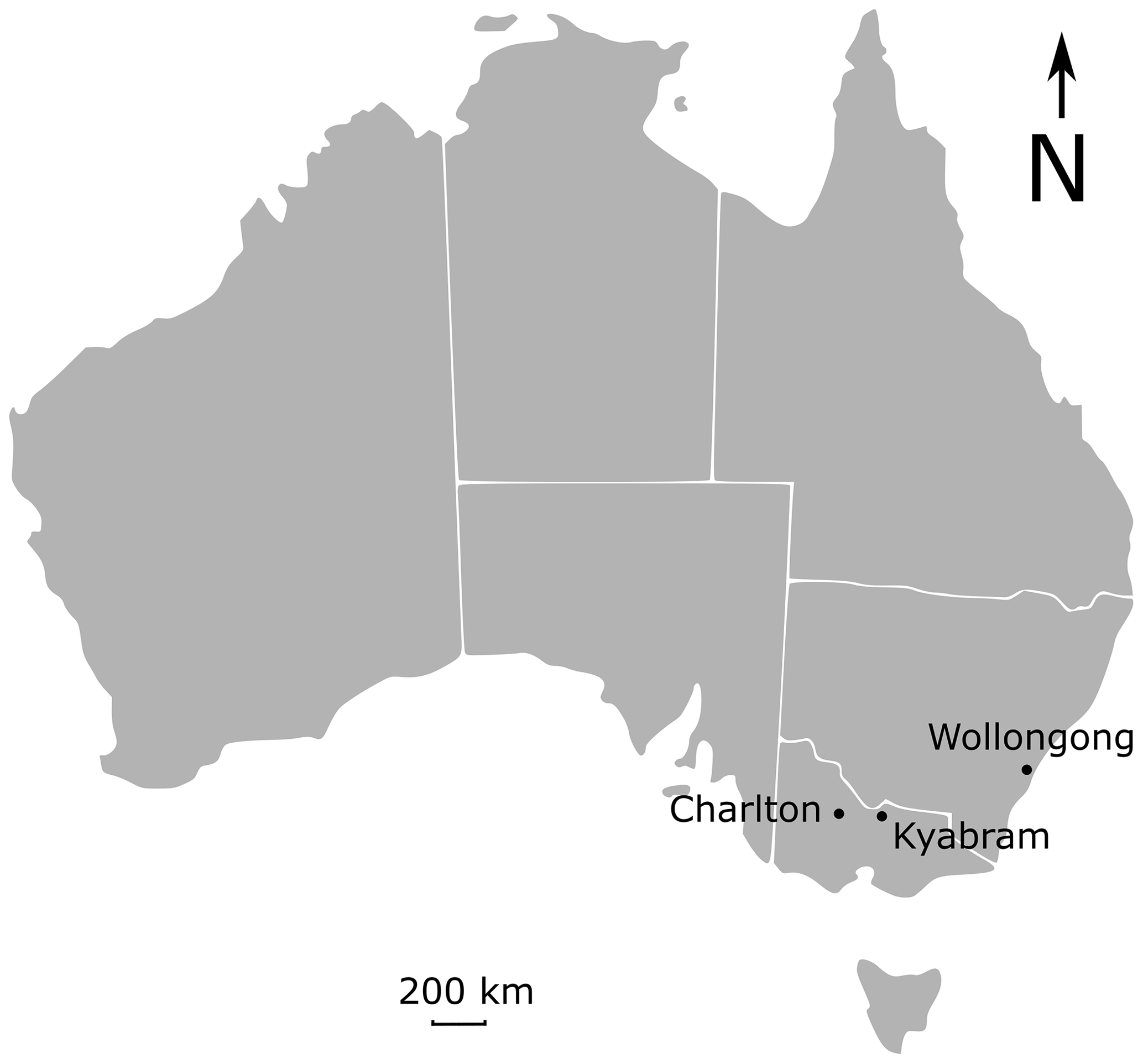
Figure 1Three experimental sites at Wollongong sports field, Kyabram research centre, and a feedlot at Charlton.
The trace gas release measurements including point and area sources were conducted at Kyabram and Wollongong, assuming that all trace gases (CH4, NH3, and N2O) disperse equally from source to open path (OP). Two OP sensors were trialled – a broadband FTIR spectrometer (OP-FTIR) and a single wavelength laser-based instrument (OPL). Besides the gas release measurements, two OP-FTIR sensors also conducted a side-by-side comparison of measuring gas mole fractions from cattle pens at a commercial beef cattle feedlot. A summary of these trials is shown in Table 1.
Table 1Summary of field measurements at Kyabram, Wollongong, and the Victorian feedlot. Target gases, instrumentations used for the studies, and study durations are also shown.
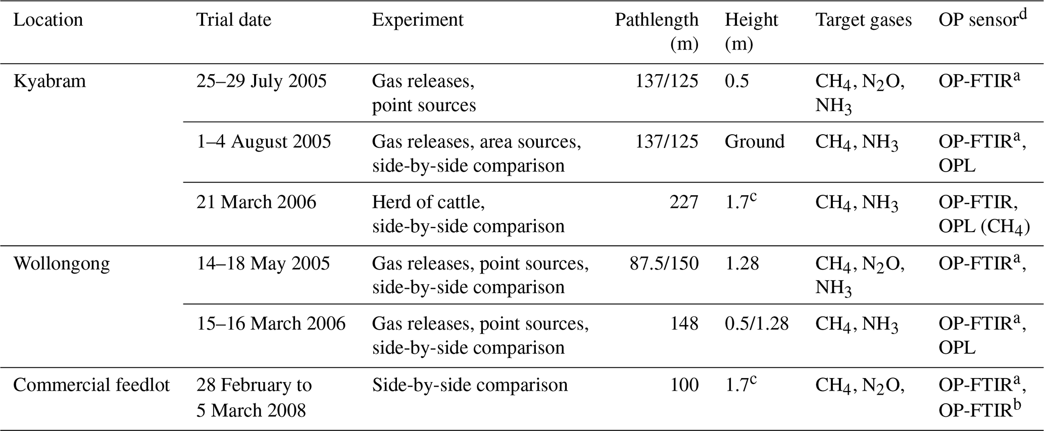
a Bomem. b Bruker. c Cattle were the main CH4 source, the average cattle height was 1.7 m. d The path length for all OP sensors was 1.5 m above the ground.
2.2 Gas release experiments
The underlying principles of the method and the accuracy and precision of the OP-FTIR and laser spectrometers were tested at Kyabram and Wollongong using releases of CH4, N2O, and NH3 at known rates from a common point or area source.
We first conducted the gas release measurements at Kyabram during a period of suitable conditions of steady wind and near neutral stability, and there were no other strong sources of CH4, N2O, and NH3 nearby. Gas release points (sources 1 and 2) were located to the west of the OP-FTIR path 1, which ran north–south along the fence line (Fig. 2). Area sources (sources 3 and 4) were located to the north of OP-FTIR path 2, which ran in a northwest–southeast direction (Fig. 2). The OPL sensors (NH3 and CH4) were set up on the north and south parallel to OP-FTIR path 2, respectively (Fig. 2). The path height for all OP sensors was 1.7 m above ground level, and the measurement path lengths were 137 and 125 m (two-way path) for paths 1 and 2, respectively. The gas release heights varied from ground level (area sources) to 0.5 m above ground level (point sources). The layout of sources and open-path geometries at Kyabram are summarized in Fig. 2. A summary of the gas release times, source types, and OP sensor measurement paths used at Kyabram is shown in Table 2.
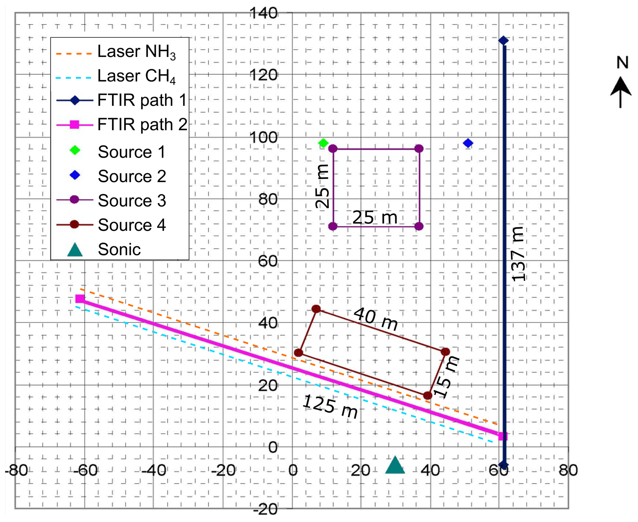
Figure 2Point and area gas release sources and OP sensor path geometries (distances in m) at Kyabram in July–August 2005. Point source 1 is in green and 2 is in blue. Area source 3 is 25×25 m, and area source 4 is 40×15 m. The OP-FTIR measurement path lengths 1 and 2 were 137 and 125 m (two-way path), respectively. OPL NH3 and CH4 sensors were parallel to OP-FTIR path 2 (dashed yellow and blue lines respectively). Sonic anemometer was located to the south of the site (dark green triangle).
Table 2Gas release times, rates, and source types for controlled release experiments at Kyabram DPI (July–August 2005). Mass flows measured in standard litres per minute (21 ∘C and 1 atm) have been converted to milligrams per second (mg s−1). LT denotes local time.
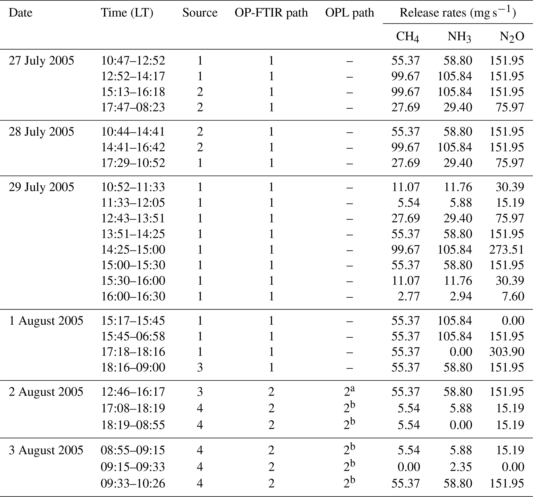
a OPL NH3 sensor only. Laser path was located 3 m north of
path 2.
b OPL NH3 and OPL CH4 sensor. OPL CH4 path was
located 3 m south of path 2.
During the point-source release trials, one OP-FTIR was set up on path 1. CH4 and NH3 were released at 9 standard litres per minute (slpm), and N2O was released at 5 slpm from a single release point over a 3 d study (1–3 August 2005) (Fig. 2). These were point sources and not distributed as cattle or soil would be. The aim was to show that the known fluxes can be retrieved from the measurements for all three gases. In this case it is permissible to have higher emissions than those typical in the field to minimize uncertainty due to background variability.
The first trial of area source release measurements was undertaken on the evening of 1 August 2005 using the 25×25 m area source (source 3) and path 1. Unfortunately, wind conditions were dominated by eastern winds, meaning that very little of the released plume crossed the measurement path. Subsequently, a period in the middle of the day with source 3 and path 2 was employed using the lasers (NH3 only) and one OP-FTIR spectrometer. The OP-FTIR spectrometer was set up on path 2, and laser NH3 sensors were run parallel 3 m north of the OP-FTIR path. Thereafter, the area source 4 (40×15 m) and path 2 were used coupled with the lasers (NH3 and CH4) and the OP-FTIR. Two OPL_CH4 lasers were located 8 m downwind from the area source, two OPL_NH3 sensors were run parallel 2 m downwind of area source, and OP-FTIR was at 5 m downwind of the source at the same time (Fig. 2). The path height for all OP sensors was 1.7 m, and the measurement path lengths were 137 and 125 m for paths 1 and 2, respectively. The different path length was determined depending on the factors of wind conditions (direction and wind speed) and the distance between the path length and source area. Given the constant wind direction, the longer pathlength was needed when the measurement path was further away from the source so that the gas plume could pass by most of the OP measurement path.
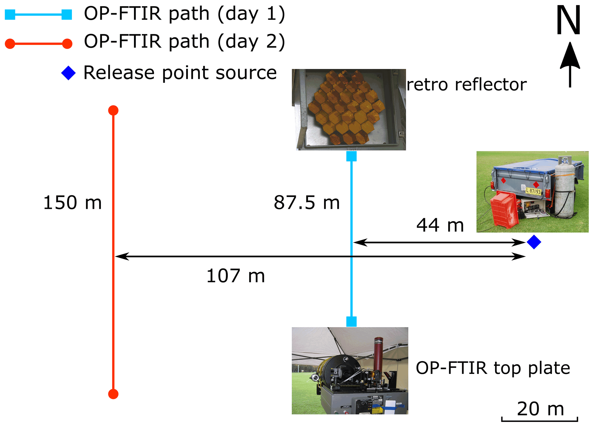
Figure 3Point gas release sources and OP-FTIR path geometries (distances in m) at Wollongong in August 2005. The OP-FTIR measurement path lengths at days 1 and 2 were 87.5 and 150 m (two-way path), respectively. Three (0.635 cm) tubes coming from three tanks (CH4, natural gas; NH3 and N2O) bundled together on a stake at the release height of 1.28 m above ground level.
The OP-FTIR was also examined at Wollongong sports field during a release trial for 2 d (Fig. 3). NH3, CH4, and N2O were released at the point source (1.28 m above ground level). The path length of OP-FTIR and its distance from the source were initially 87.5 (two-way path) and 44 m, respectively; the OP-FTIR spectrometer was then moved further away from the source: 107 m from the source with a longer measurement path of 150 m (two-way path).
Furthermore, to check the long-term performance of precision and accuracy of the instruments, we conducted side-by-side measurements to evaluate sensor differences at Wollongong and a commercial feedlot northwest of Victoria. During the intercomparison of OPL and OP-FTIR at Wollongong, the OPL sensors (two for CH4 and two for NH3) and the Bomem OP-FTIR spectrometer recorded mole fractions over a path length of 148 m (two-way path) before and after the gases were released. At the commercial feedlot (Fig. 4), two OP-FTIR spectrometers were run side-by-side. Mole fractions of CH4, N2O, and NH3 were simultaneously measured for 6 d with the path length of 100 m (two-way path) and measurement height of 1.5 m above the ground. Flasks (600 mL) were evacuated prior to gas sampling. For each sample day during stable boundary layer conditions (Monin–Obukhov length L, L≅ 0–10 m), air samples were collected simultaneously at three points (0, 50, 100 m from the spectrometer) along the measurement path. A total of 14 samples over a 5 d period were collected. The air samples were analysed using a closed-path FTIR spectrometer at the off-site laboratory at University of Wollongong, which has been calibrated with the standard gases CH4 and N2O (Griffith et al., 2012). The concurrent mole fractions of CH4 and N2O measured by two FTIR spectrometers were compared to those of air samples.
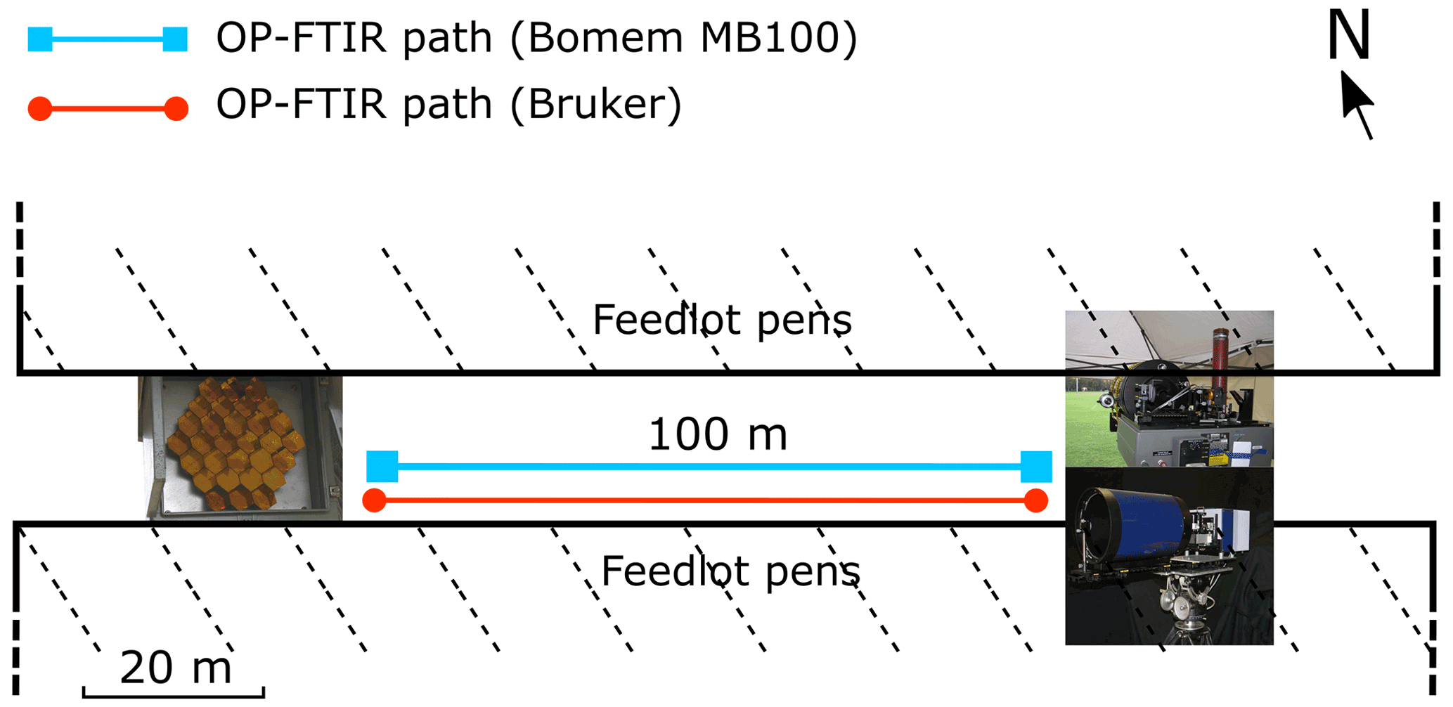
Figure 4Two OP-FTIR spectrometers (Bomem MB100 and Bruker) during side-by-side operation in a commercial feedlot in Victoria in February 2008.
2.3 Gas release system
The controlled gas releases were of NH3 (>99 %, BOC refrigeration grade, Australia), CH4 (compressed natural gas, 89 % CH4, Agility, Australia), and N2O (>99 %, BOC instrument grade, Australia) supplied from high-pressure cylinders. Each of the gas flows was controlled by a mass flow controller with ±2 % full-scale repeatability (SmartTrak™ series 100, Sierra Instruments Inc., California, USA). Each gas cylinder was connected to the mass flow controller with (0.635 cm) nylon tubing, and the gas outflow from each mass flow controller was released to the atmosphere through another length of nylon tubing. Each gas flow controller was scaled for the gas measurement using the manufacturer's data. Controlled gas flow rates were logged every minute using a data logger (dataTaker, Melbourne). For point-source emissions, the outlets of the three gases were co-located at a release height of 0.5–1.28 m above ground. For surface area emissions, the flows were fed into a length of drip-irrigation tubing (Miniscape, 8 mm) with valve holes every 2.5 m and spread over a 25×25 m or 40×15 m grid at ground level.
2.4 Open-path spectrometers
2.4.1 Open-path lasers
Four open-path lasers (OPLs; GasFinder2.0, Boreal Laser Inc, Edmonton, Alberta, Canada) were used. Two units (1012 and 1013) measured CH4, and the other two (1015 and 1016) measured NH3. Each OPL was associated with a remote passive retro reflector that delineated the path. The OPL contains a transceiver that houses the laser diode, drive electronics, detector module, and micro-computer subsystems. Collimated light emitted from the transceiver traverses the OP to the retro reflector and back. A portion of the beam passes through an internal reference cell. Trace gas mole fraction in the optical path is determined from the ratio of measured external and reference signals. Sample scans are made at approximately 1 s intervals, and the data were stored internally as 1 min averages. Transceivers are portable, tripod-mounted, and battery-operated (12 VDC). The retro reflector is tripod-mounted and composed of an array of six gold-coated 6 cm corner cubes with effective diameters of approximately 20 cm. The alignment of transceiver and retro reflector is straightforward and generally stable for several hours over path lengths up to 500 m. The nominal sensitivity of the laser units is 1 part per million volume per metre (ppmv-m), corresponding to 0.01 ppmv for a 100 m path.
2.4.2 Open-path FTIR
There were two different OP-FTIR units used in these studies. The first unit consisted of a Bomem MB100-2E OP-FTIR spectrometer (ABB Bomem, Quebec, Canada) and a modified Meade 30.5 cm diameter LX200 Schmidt–Cassegrain telescope, which were assembled at the University of Wollongong along with software (Tonini, 2005). Operationally, the transfer optics take the modulated infrared radiation from the FTIR through the telescope to reduce beam divergence to a set of retro reflectors placed at some distance away, collect the returned radiation, and focus the radiation onto a liquid-nitrogen-cooled mercury–cadmium–telluride (MCT) detector. A Zener diode thermometer (type LM335) and a barometer (PTB110, Vaisala, Helsinki, Finland) provide real-time air temperature and pressure data for the analysis of the measured spectra. The spectrometer is operated at 1 cm−1 resolution, and one spectrometer scan takes approximately 4 s (13 scans per minute). For acceptable signal to noise ratios, scans are generally averaged for at least 1 min. Immediately following each measurement, the spectrum is analysed, and calculated mole fractions are displayed and logged in real time, together with ambient pressure and temperature. Operation is continuous and fully automated by the software to control the spectrometer, data logging, and spectrum analysis (Paton-Walsh et al., 2014). Under normal operation the detector must be re-filled with liquid nitrogen once per day, and occasional re-alignment of the spectrometer on the tripod may be required depending on the stability of the tripod footings.
Quantitative analysis to determine trace gas mole fractions from OP-FTIR spectra is based on non-linear least squares fitting of the measured spectra by a computed spectrum based on the HITRAN (high-resolution transmission molecular absorption) database of spectral line parameters (Rothman et al., 2009, 2005) using a model calculation (Griffith, 1996). The OP-FTIR spectrum is iteratively calculated until a best fit to the measured spectrum is obtained. The mole fraction of absorbing species in the OP is obtained from the best-fit input parameters to the calculated spectrum (Griffith, 1996; Smith et al., 2011). The OP-FTIR spectrometer measures the broadband IR spectrum simultaneously over the range 600–5000 cm−1. The three separate spectral regions (N2O, 2130–2283 cm−1; CH4, 2920–3020 cm−1, and NH3, 900–980 cm−1) are extracted from the broadband spectrum and analysed separately for each target species.
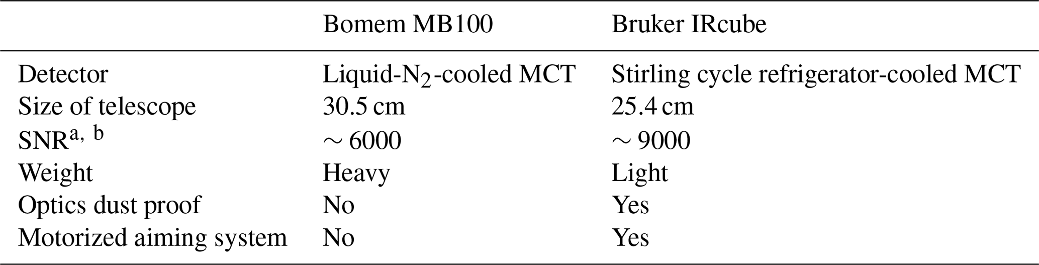
The second OP-FTIR unit was the Bruker IRcube spectrometer (Matrix-M IRcube, Bruker Optics, Ettlingen, Germany) that was developed based on the same principle as the Bomem spectrometer (University of Wollongong) (Paton-Walsh et al., 2014; Phillips et al., 2019). This Bruker OP-FTIR spectrometer replaced the liquid nitrogen (N2) system with a Stirling cycle mechanical refrigerator, and a 25.4 cm diameter telescope and a secondary mirror were built to create a 25 mm parallel beam to extend the measurement path up to 500 m. The analytical spectral regions are the same as Bomem MB100. More details of the Bruker IRcube spectrometer can be found in Bai (2010). The system parameters from both OP-FTIR spectrometers are summarized in Table 3. Recently, a custom-made motorized tripod head was installed to allow the spectrometer to be aimed at multiple paths where the retro-reflectors were separated vertically or horizontally (Bai et al., 2016; Flesch et al., 2016).
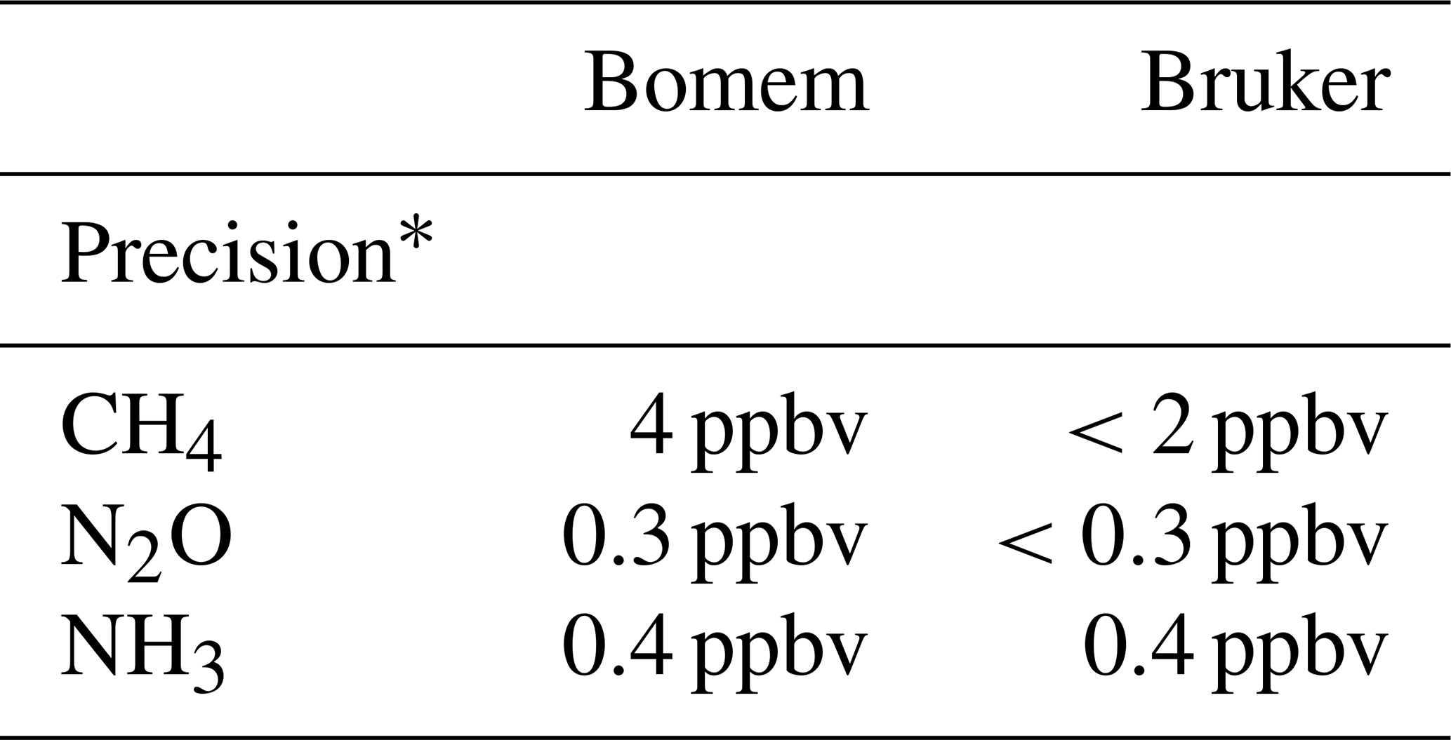
Table 3The system parameters between OP-FTIR Bomem MB100 and Bruker IR cube spectrometers.
a SNR, signal to noise ratio. A transmission spectrum is
calculated by taking ratios of two successive spectra and measuring root
mean square (rms) noise at a spectral region of 2500–2600 cm−1.
b Measured over 100 m path length (two-way path).
2.5 Dispersion modelling (WindTrax)
To infer emission source strengths or fluxes from atmospheric mole fraction measurements, we require a means to quantify atmospheric transport and dispersion of the target trace gases between source and measuring point. Our approach is to infer area-averaged surface fluxes (in excess of background) from measured line-averaged mole fractions by using a backward Lagrangian stochastic (bLs) model as developed by Flesch et al. (2004, 1995). The bLs model is capable of handling sources of arbitrary size and geometry. The model is encoded in the commercially available software package WindTrax (version 1.0, Thunder Beach Scientific) (Crenna et al., 2006). The inputs for WindTrax bLs model include the measured mole fraction and sonic anemometer measurements of wind speed and direction, stability, and turbulence, as well as other micrometeorological parameters. The WindTrax bLs model simulates the backwards trajectories of molecules sensed in the optical path. The instrument tower (in the source area) provides the information necessary to calculate the trajectories. In this study, 50 000 parcels are released and propagated backward to build up a statistical distribution of trajectories from which source strengths can be calculated. “Touchdowns” are partitioned into those originating in the source area and those from the background. This allows the net flux of particles across the path to be separated into contributions from source and background level.
Similar to the studies in McGinn et al. (2006), we predicted tracer release rates by measuring downwind mole fractions from area sources using the bLs model. We measured downwind mole fractions before and after releasing each trace gas, and the difference in the mole fractions was then used to determine the source release rate. However, WindTrax cannot be used to carry out backward simulations for point sources (i.e. conversion of mole fraction data to fluxes). It can, however, predict downwind mole fraction from estimated release rate using the model running in forward mode.
2.6 Weather data
A three-dimensional (3-D) sonic anemometer (CSAT3, Campbell Scientific, Logan, Utah, US) with data logger (CR5000, Campbell Scientific, Logan, Utah, US) was used to record wind speed and direction along with the turbulence statistics at a frequency of 10 Hz. The 15 min interval data were then transformed to friction velocity (u*), atmospheric stability (L), and surface roughness length (z0) as half-hour averages, determining the time increments of OP sensor data.
2.7 Data filtering criteria
Poor measurements of mole fractions were not counted when the spectrum signal intensities were <0.2 (spec. max) for OP-FTIR, light level less than 5000 or greater than 12 000, and R2<0.90 for OPL. Following Flesch et al. (2004), we excluded the data that were associated with error-prone WindTrax fluxes (low-wind conditions and strong stable or unstable stratification): wind speed <2 m s−1, , and fraction of “touchdown” <0.1.
3.1 OP-FTIR measurements
The wind was steady from the north-northwest (325–335∘) at 1.8–3.5 m s−1 over the measurement period of 14:45–16:30 local time (LT) on the 27 July 2005 Kyabram trial (T1). Between 14:45 and 15:10 LT and after 16:20 LT background data were collected. Figure 5 shows the OP-FTIR measurements of all three gases during this period, expressed as path-averaged mole fractions in parts per billion volume (ppbv) after subtracting the background level. We found that the enhanced mole fractions of the source (downwind minus upwind mole fractions) of CH4, N2O, and NH3 measured by OP-FTIR followed a similar correspondence.
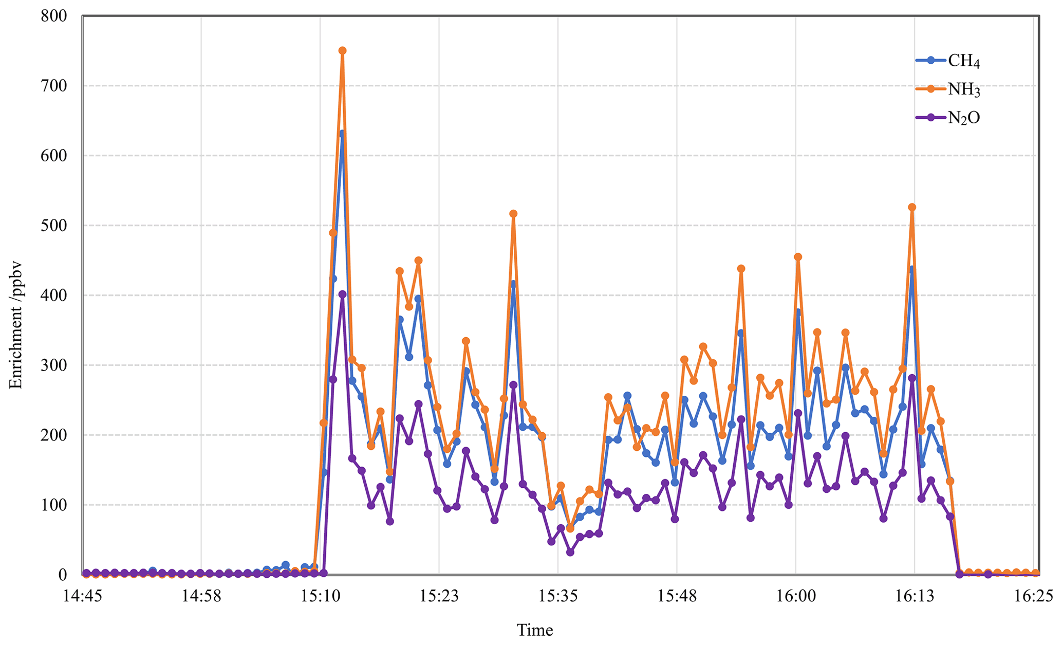
Figure 5Measured OP-FTIR 1 min averaged mole fractions of CH4, N2O, and NH3 after subtracting the background levels during a point-source gas release experiment at Kyabram on 27 July 2005.
We also found that the mean measured OP-FTIR mole fraction of CH4:N2O was 1.61 compared to the release rate ratio of 1.60, and the mean measured mole fraction of NH3:N2O was 1.84 (release rate ratio was 1.80). The release rates with measured regression slopes for all trial release measurements made at both Wollongong and Kyabram are shown in Table 4. In all but three cases the ratio was within 1 %–8 % of the 1:1 ratio. The OP-FTIR system uses no calibration gases, but system calibration is based on the accuracy of the HITRAN line parameters and the MALT (Multiple Atmospheric Layer Transmission) spectrum model. Typical absolute accuracy is 1 %–5 % depending on species and OP set-up, with precision (reproducibility) normally much better than 1 % (Esler et al., 2000). The use of MALT synthetic spectra based on quantum mechanical parameters has been shown to yield accurate results (within 5 % of true amounts) when tested against calibration gases in a 3.5 L multi-pass gas cell with 24 m optical path length (Smith et al., 2011). In each case of disagreement, the correlation remains strong, and the systematic differences can reasonably be attributed either to a leak in the release system or in the case of low NH3 to the losses by adsorption at the (wet) ground over the longer release measurement distance during the experiment.
Table 4Comparison of the release rate ratios and OP-FTIR-measured enhanced mole fractions for the controlled release gas measurements.

a No data due to CH4 gas flow problems during this time period.
b Ratio that is not in agreement with the controlled release ratio (ρ<0.05).
c Time of measurement period represents local time.
d The measured mole fraction is from 17:30 to 00:30 LT because of an increased background effect from 00:30 to 08:30 LT.
3.2 OP-FTIR error assessment
From measurements before and after release, the measurement precision and accuracy of the OP-FTIR measurements were assessed (Table 5). Measured background mole fractions of CH4 and N2O at Kyabram were similar to the clean air values measured at the Cape Grim Baseline Air Pollution Station in Tasmania. The differences between measured background values at Kyabram and Cape Grim were <3 % and consistent with the known absolute uncertainty in OP-FTIR calibration (1 %–5 %, the accuracy of MALT and HITRAN).
Table 5Measurement precision and comparison with clean air composition for OP-FTIR measurements during the trace gas release trial experimental period at Kyabram. Background mole fractions measured at Cape Grim Baseline Air Pollution Station in Tasmania at the same time are also shown.

Note: 1σ is standard error.
Regression analyses showed a residual scatter (standard deviation of the residuals) around the regression line of typically 8 ppbv for NH3:N2O and 18 ppbv for CH4:N2O (Fig. 6). This scatter was significantly larger than the measurement precisions (Table 5) and suggested that the fundamental limit to the accuracy and applicability of the OP technique came from variability in the dispersion of the trace gases by atmospheric turbulence – i.e. even when co-released at nominally the same point, statistical fluctuations ensured that gas parcels did not follow exactly the same paths. It thus appeared that measurement precision was not the limiting factor and was sufficient for the purposes of the measurements. Background variations and turbulence statistics were the error-limiting factors in the OP measurements.
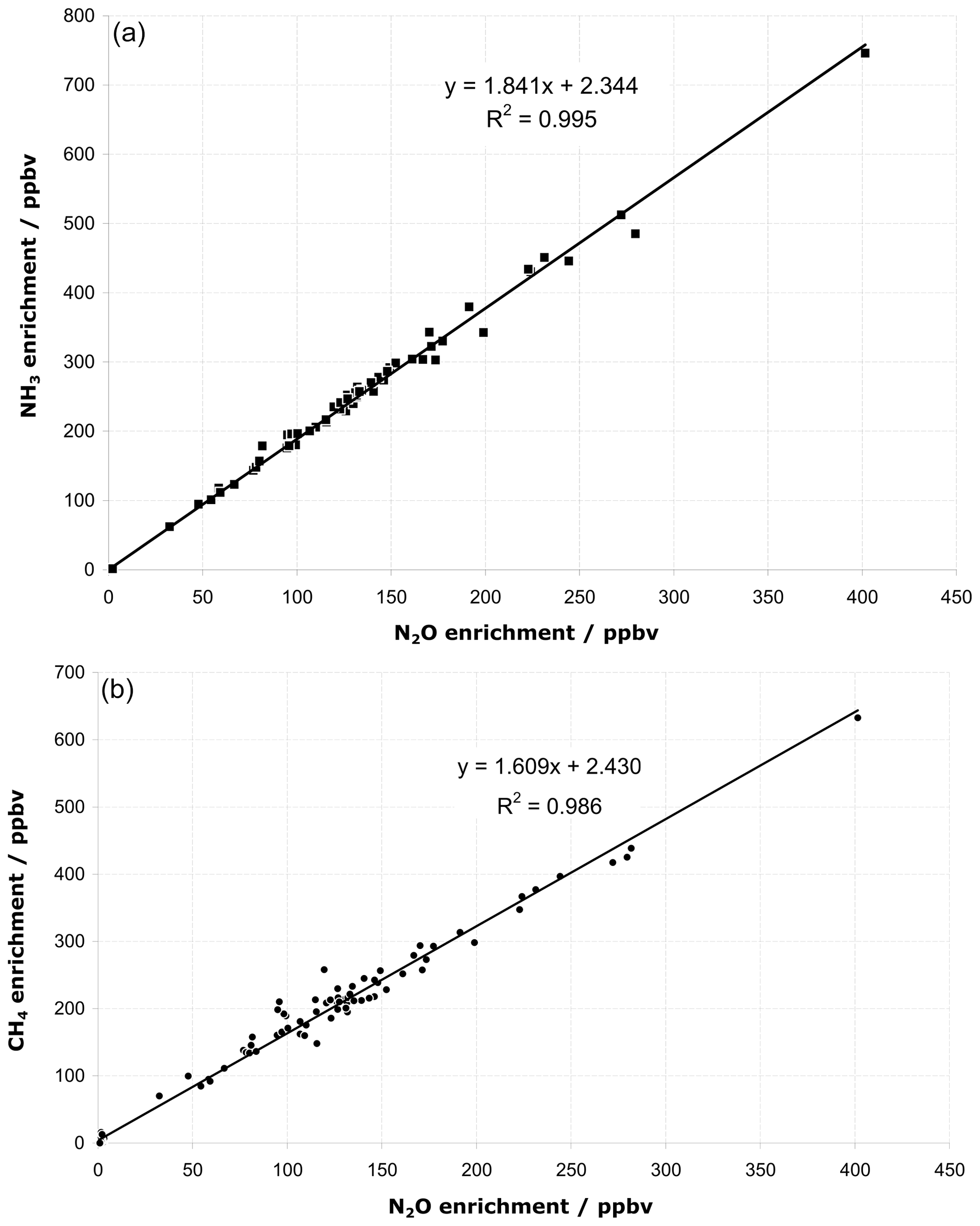
Figure 6Linear regression analysis of the OP-FTIR-measured enrichments shown in Fig. 5 between 14:45 and 16:25 LT of NH3 vs. N2O (a) and CH4 vs. N2O (b).
3.3 Comparisons of OPL and OP-FTIR measurements
The 1 min averages of CH4 and NH3 mole fractions measured by OPL (one unit for CH4, 1012, and two units for NH3, 1015 and 1016) and OP-FTIR over the period of controlled gas release at Kyabram (T2) were compared (Fig. 7).
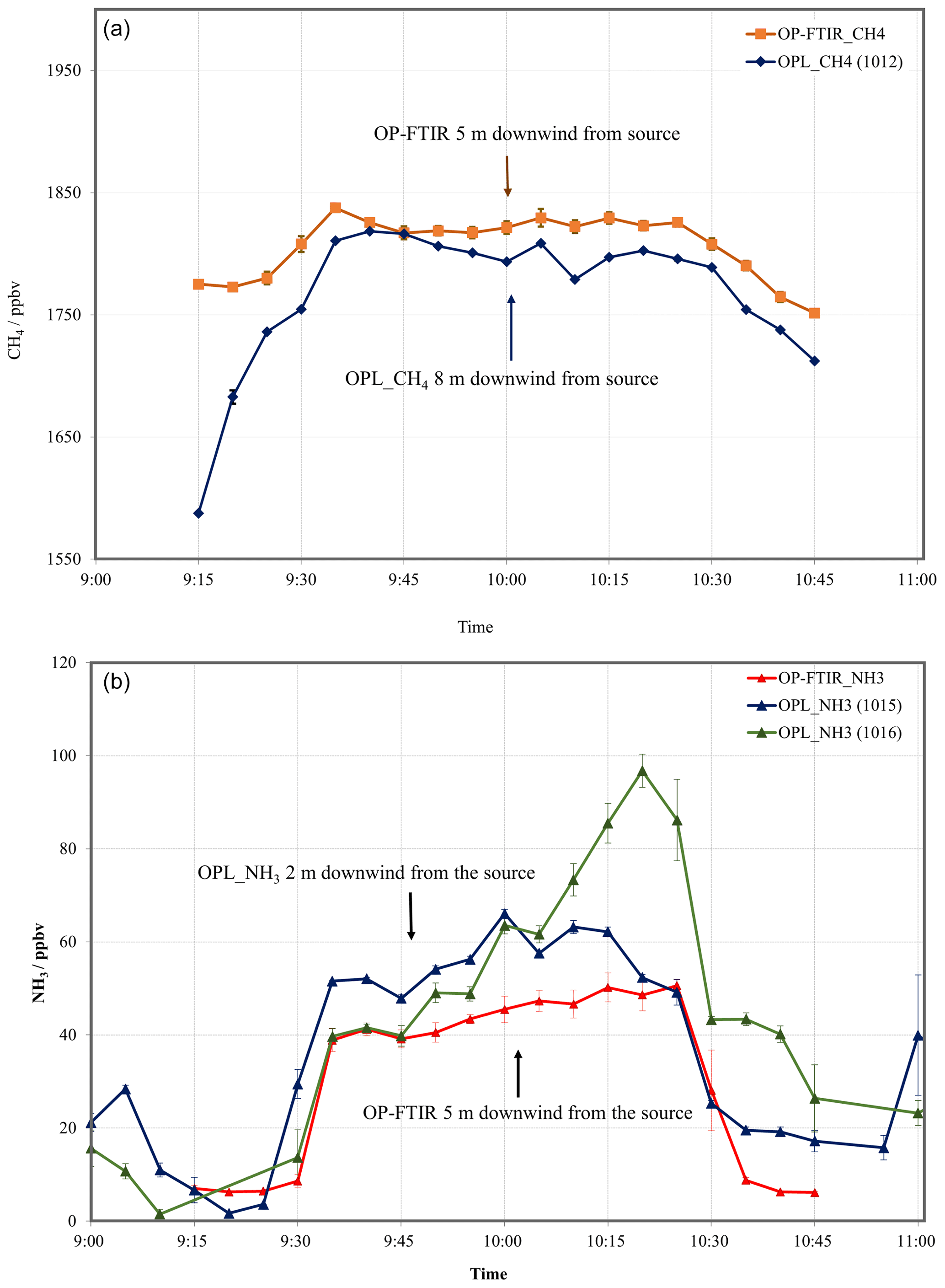
Figure 7The 5 min averages of CH4 (a) and NH3 (b) mole fraction measurements from the OP-FTIR and OPL downwind of a ground-level grid source 40×15 m wide (path length =125 m) at Kyabram on 3 August 2005 (T2). The error bars represent the standard error.
In general, the OPL_CH4 and OPL_NH3 tracked the OP-FTIR measurements; however, the OPL_NH3 did not have a stable baseline (fluctuations of around 15 ppbv) and showed a significantly lower signal to noise ratio than that of the OP-FTIR. Offsets in the measured mole fractions may be due to the relative positions of the emission source and the instruments.1
A second intercomparison between the CH4 OPL (1012 and 1013) and OP-FTIR measurements at Wollongong is shown in Fig. 8. The 30 min averaged OPL_CH4 tracked the OP-FTIR measurements but recorded lower values, with background CH4 lower than the Cape Grim background of 1738 ppbv (Table 5). There were also discrepancies between the two lasers: the 1013 unit was more stable and measured higher values than that of the 1012 unit. Flesch et al. (2004) report a similar problem with the long-term stability of CH4 lasers and implement a rigorous calibration strategy, suggesting recalibrating several times over the course of a field campaign. Laubach et al. (2016) reported the temperature-dependent effect on OPL CH4 performance. The implementation of a routine calibration protocol would account for these offsets as long as they were consistent. However, fluctuations of around 10 ppbv characterized the limit of the resolution of the instrument.

Figure 8The 30 min averaged CH4 mole fraction measured by OP-FTIR and both OPL units (1012 and 1013) positioned side-by-side (path length =148 m) at Wollongong site. Error bars denote the standard error.
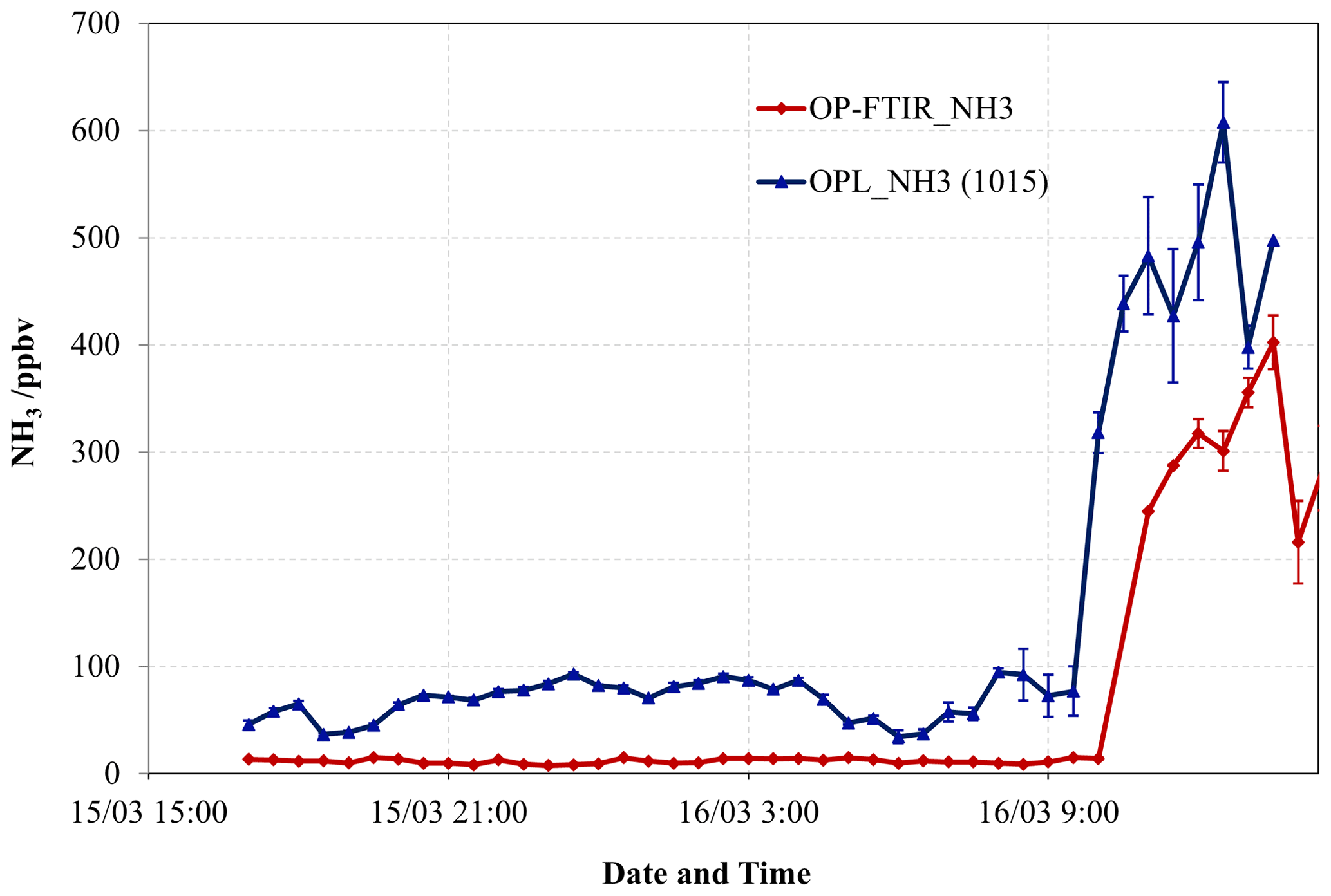
Figure 9The 30 min averaged NH3 mole fraction measured by the OP-FTIR spectrometer and OPL unit 1015 positioned side-by-side (path length =148 m) at the Wollongong site. Error bars denote the standard error of the 30 min means.
We also compared 30 min averages of NH3 measurements at Wollongong (Fig. 9) prior to and after the gas release (NH3 release rate at 5 slpm). Prior to the gas release (15 March 2006), the laser mole fractions at background levels appear elevated, while the FTIR showed a greater stable baseline; this suggested clearly that the resolution of the lasers was no better than the 1 ppmv-m specified by the manufacturer. After the NH3 was released (after 10:00 LT 16 March 2006), the path-averaged mole fraction rose above 0.1 ppmv, but the OPL_NH3 (1015 unit) measurements were less erratic at these elevated mole fractions. This indicated the detection limit of the OPL_NH3 was no better than the 1 ppmv-m specified by the manufacturer. Rigorous calibration should account for OPL offsets. However, there remained major discrepancies between measured mole fractions of the OPL_NH3 and OP-FTIR. Clearly, this reflected that the OPL_NH3 is not suited to monitor background mole fractions of NH3 (typically <10 ppbv). Moreover, it is only likely to be feasible in situations where there are very large enrichments in NH3 as the precision is no better than 10 ppbv over 100–200 m paths.
3.4 Comparisons of two OP-FTIR spectrometers
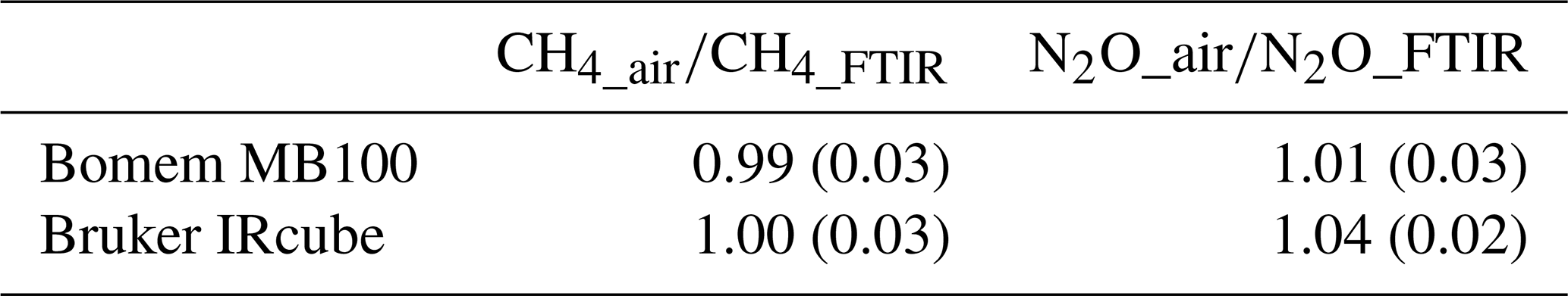
The ratios of measurement between air samples and FTIR (Bomem and Bruker) are shown in Table 6. We found that CH4 results from Bruker FTIR were more reliable in stable conditions than N2O values but comparable to Bomem FTIR results. We also calculated the measurement precisions over a Bruker IRcube which showed higher measurement precision of CH4 and N2O than Bomem MB100 but was similar to NH3 precision (Table 7).
Table 6Ratios of mole fractions of CH4 and N2O between air samples and OP-FTIR including Bomem MB100 and Bruker IRcube spectrometers*.
* Mean (standard deviation). The measurements were conducted at stable background conditions for 6 d at Charlton, Victoria. The pathlength was 100 m (two-way path), and measurement height was 1.5 m above ground level.
Table 7The precisions of CH4, N2O, and NH3 for OP-FTIR Bomem MB100 and Bruker IR cube spectrometers.
* Measured over 100 m path length (two-way path).
3.5 Trace gas recoveries with WindTrax
3.5.1 OP-FTIR
We ran WindTrax bLs model to calculate trace gas fluxes during a period in the middle of the day on 2 August 2005 with source 3 (25×25 m) and path 1 with the mole fraction measured by the OPL (NH3 only) and OP-FTIR (Fig. 2). Meteorological conditions varied significantly throughout the period, from unstable ( m) at the start to slightly stable (L≅50 m) towards the end. Wind speed averaged 2.5 m s−1, and wind direction was relatively constant at 30∘. We assumed the background mole fraction was constant: 1755, 324, and <1 ppbv for CH4, N2O, and NH3, respectively (Table 5). The results of the WindTrax bLs recovery of flux using OP-FTIR mole fractions are illustrated in Appendix Fig. A1 as the ratio of calculated (QbLS) to known (Q) flux. Recoveries of N2O flux were generally good although low (average recovery is 0.93). This may be due to an issue with the operation of the grid source (such as the distribution of gas). NH3 recovery was even lower (mean of 0.71). In this case the adsorption of NH3 on to the grass may also have contributed to a reduction in measured mole fraction (Tonini, 2005). Apart from the first 30 min period, which appeared to have been affected by an elevated background mole fraction, CH4 flux recoveries were much lower (mean of 0.52) than for the other gases.
We also calculated trace gas fluxes with area source 4 (40×15 m) and path 2 (Fig. 2). Low release rates were employed until the final hour when they were increased by an order of magnitude. Meteorological stability was quite high at the start of the period (L≅ 0–10 m), gradually becoming less stable during the night and into morning. Wind speed was correspondingly low (1.5 m s−1) at the start and increased to 4 m s−1 by the end of the period, and wind direction swung from east-northeast to north-northeast. The results for N2O are shown in Appendix Fig. A2 and for CH4 and NH3 in Appendix Fig. A3. The results for the N2O fluxes were very encouraging. There were some intervals where retrievals were greater than 1 at the start of the period and 2 towards the end. The latter occurred at a time when wind speed increased, and conditions swung from neutral to unstable. Excluding these intervals provided an average ratio of 1.04, with a standard deviation of 0.15. Few points were available for NH3 as it was not released during the night. The average for the last two data points was 0.96. Once again, CH4 retrievals were problematic due to variations in the background mole fraction. With this source geometry and wind field a change in flux of 1 mmole s−1 results in a path-averaged change in mole fraction of 50 ppbv. Small variations in the background thus translated to large mass flux changes (e.g. 1 ppbv corresponds to mmole s mg s−1 or 5.8 % of the released flux of 5.5 mg s−1). Under these conditions accurate flux calculation requires a well-defined background mole fraction measurement.
3.5.2 Lasers (NH3)
Figure A4 shows the results of the same controlled release experiment described in the OP-FTIR section above. Again, the bLs model was used to predict the NH3 emission source strength based on OPL NH3 line-averaged mole fraction measurements.
Although the correlation was reasonable, unlike the recoveries calculated from the OP-FTIR data, the ratio of predicted to known source strength was greater than 1 for these data. This was not altogether surprising given the consistently inflated NH3 mole fractions measured by the OPL sensors.
3.6 Herd emissions using OP-FTIR, OPL, and WindTrax
The study was conducted at Kyabram DPI on 21 March 2006 (Appendix Fig. 5a). Appendix Figs. A6 and A7 show the fluxes of CH4 and NH3 due to a herd of 353 dairy cows grazing at Kyabram DPI on 21 March 2006, calculated using bLs model in WindTrax and OP-FTIR- and OPL-measured (for CH4) mole fractions. The calculated CH4 source was variable because the cows were wandering around the paddock (Fig. A6), which is clearly marked at the time when the cows departed the bay (Bay 8) for milking. The CH4 source strength disappeared after this time, as it should. Missing data points corresponded to periods of time when the average wind speed was less than 2 m s−1, which is when the bLs model was likely unreliable. The average calculated source strength, based on the OP-FTIR data, was 57.5 , equivalent to 292 g per cow per day. This calculation assumed a uniform background mole fraction of CH4 of 1610 ppbv. Fluxes based on the upwind and downwind OPL data were strongly correlated with the OP-FTIR results and predicted an average flux of 48.5 . The lower value probably reflected the offsets between the instruments. Atmospheric conditions of the following day were too still to reliably use the data acquired on the second day of grazing. Figure A7 showed that the OP-FTIR NH3 fluxes ranged from 0.3 to 0.8 , with average flux around 0.5 , equivalent to 0.7 gN per cow per day assuming NH3 volatilizations only occurred during the daytime (8 h). This was similar to the NH3 emission fluxes of 0.25 to 2.5 g per cow per day, measured at the same site and same season (early April) in 2004 using the combination of passive NH3 sampler and WindTrax (Denmead et al., 2020).
3.7 WindTrax sensitivity
A model sensitivity study was undertaken in order to understand how the source strength predicted by WindTrax alters with variations in a range of input parameters. No sonic anemometer data were used – instead we used simple wind speed and direction and constructed a surface layer model from local weather conditions and estimates of surface roughness. Example data from FTIR measurements in Kyabram on 21 March 2006 were used, and five input parameters were varied around the standard conditions. Table 8 below shows how the calculated source strength of CH4 from the paddock of cows varied with changes in the wind speed, stability, surface roughness, height of sensor, and temperature assumed by the WindTrax model.
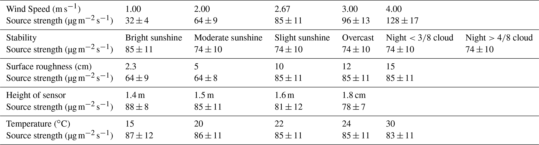
The model appeared to be quite robust with respect to height of the sensor, temperature, and stability conditions, while changing the assumed surface roughness from 5 to 10 cm altered the predicted fluxes quite markedly. The modelled source strength scaled with wind speed, so accurate meteorological data were a requirement of this technique. It should also be noted that the WindTrax model was not expected to work well when wind speed was below 2 m s−1.
3.8 The total uncertainty budget
We want to compute the total uncertainty associated with the difference in mole fraction between upwind and downwind. There are three uncertainty sources: instrument precision uncertainty, fitting uncertainty, and absorption cross-section (HITRAN) uncertainty (the latter two are fractional uncertainties and were taken from Paton-Walsh et al., 2014) (Table 9). The measurement precision is in units of parts per billion volume (ppbv), and so the fractional uncertainty that this represents will change with the trace gas mole fraction. The instrument precision uncertainty (δ) associated with upwind measurement is 1σ, and the uncertainty associated with downwind is also 1σ. We assume these errors to be independent. The instrument precision uncertainty in the difference in mole fraction between upwind and downwind is thus . We then divide this value by the difference in mole fraction to recover the relative uncertainty due to instrument precision: . . We then add in quadrature the relative measurement uncertainty due to instrument precision with the fitting and absorption cross-section uncertainties (also expressed in terms of relative uncertainty). For example, for CH4, when ΔCH4 was as low as 20 ppbv, we have a relative uncertainty of 0.28 for the instrument precision, 0.02 for fitting uncertainty, and 0.05 for absorption cross-section uncertainty. The relative uncertainty propagated across these three components is or 28.8 %. When the ΔCH4 was increased to 50 or 100 ppbv, the uncertainty declined dramatically to 12.5 % and 7.8 %, respectively. However, for N2O and NH3 the uncertainty was not limited by the mole fraction enhancement but was likely attributed to absorption cross-section uncertainty.
Table 9Total uncertainty budget.

* Δ trace gas mole fraction = (trace gas mole fraction)downwind− (trace gas mole fraction)upwind.
We have used OP systems for measuring mole fractions of CH4, N2O, and NH3, and we evaluated their performance and precision. Two OP systems for measuring line-averaged gas mole fractions have been evaluated over path lengths up to about 200 m.
The OP-FTIR system can measure multiple gases simultaneously with excellent precision, e.g. CH4, 2–4 ppbv, N2O, 0.3 ppbv, and NH3, 0.4 ppbv. As the baseline appears to be very stable, we believe the OP-FTIR technique has the accuracy for even small enrichments in GHGs. However, the apparatus remains bulky to set up in a field environment, where access to main power is often difficult. In contrast, the commercial OPL units have the advantage of being readily portable and battery-powered. This study has evaluated OPL for CH4 and NH3. These instruments have somewhat poorer precision than the OP-FTIR spectrometer of around 10 ppbv for CH4 and 15 ppbv for NH3. While the OPL should be capable of following ambient fluctuations in CH4 gas mole fractions, the resolution of the NH3 OPL was greater than the background mole fractions of NH3, resulting in large errors when calculating fluxes. WindTrax provided accurate recoveries of known test gas releases from the source area and appears to be well suited for the analysis of OP measurements under suitable meteorological conditions. These experiments highlighted the importance of having a robust background mole fraction measurement.
Our studies also suggest that the OP-FTIR and OPL are suitable to measure typical enrichments in CH4 and NH3 from agriculture and useful in calculating fluxes from a variety of agricultural activities, such as free-ranging cattle and sheep. We recommend that they are also well-suited to concentrated sources such as feedlots, animal sheds, and small enclosures. The OP-FTIR system should also be suited to emissions of CH4 from rice-growing sources and wastewater lagoons. The OP-FTIR system provides excellent NH3 precision suitable for measuring paddock-scale emissions from fertilizer (urea, effluent) applications and dung and urine patches. The high detection limit and long-term stability of OP-FTIR enables us to measure small changes in N2O emissions at large scale from fertilizer treatment or dairy pastures. The OPL NH3 has a low resolution of free-air mole fractions, in particular weak sources, in which the enhanced values are low and the error in background is minimized.
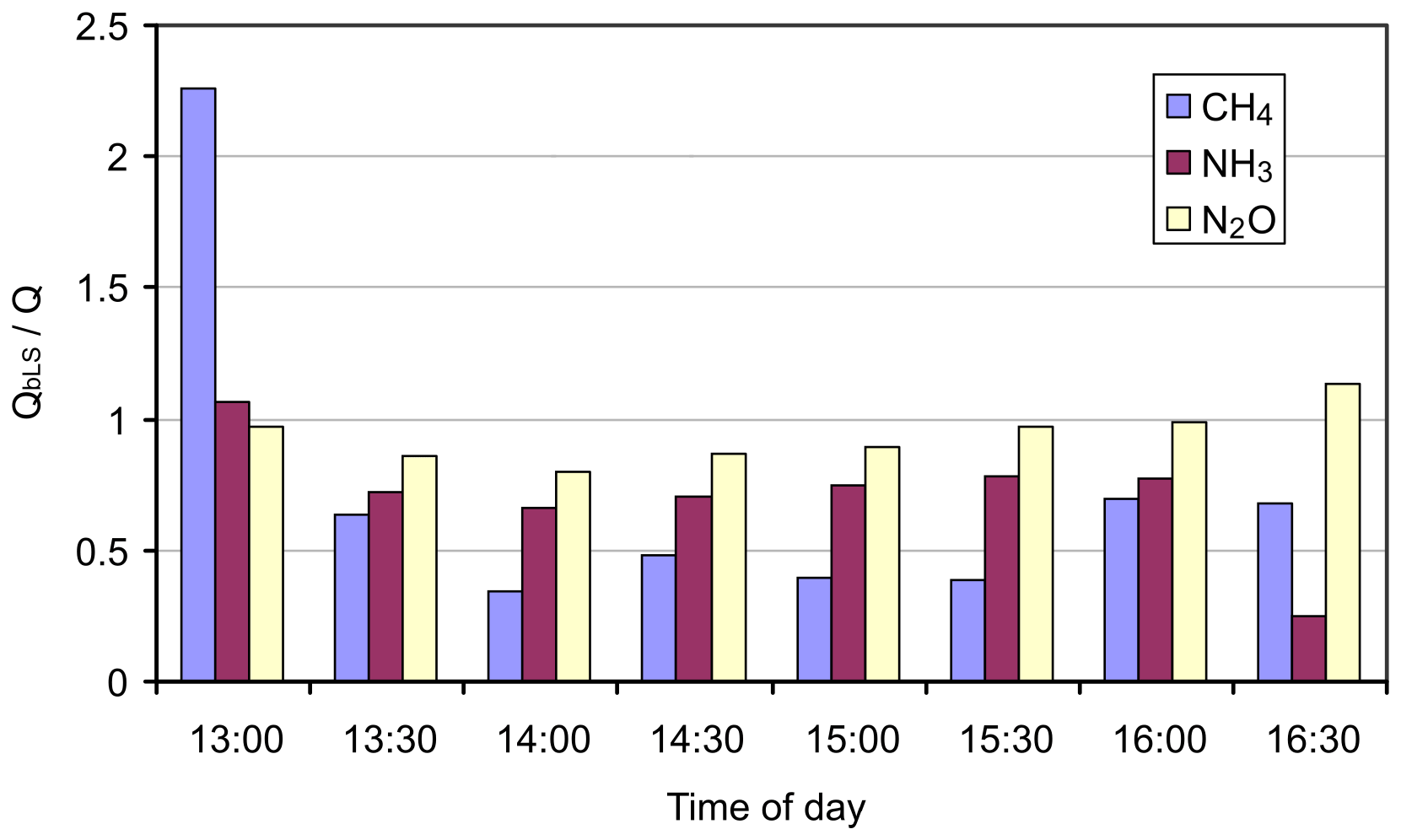
Figure A1Ratio of predicted to known flux for ground-level 25×25 m area source (source 3), using OP-FTIR mole fractions and measurement path 2 on 2 August 2005.
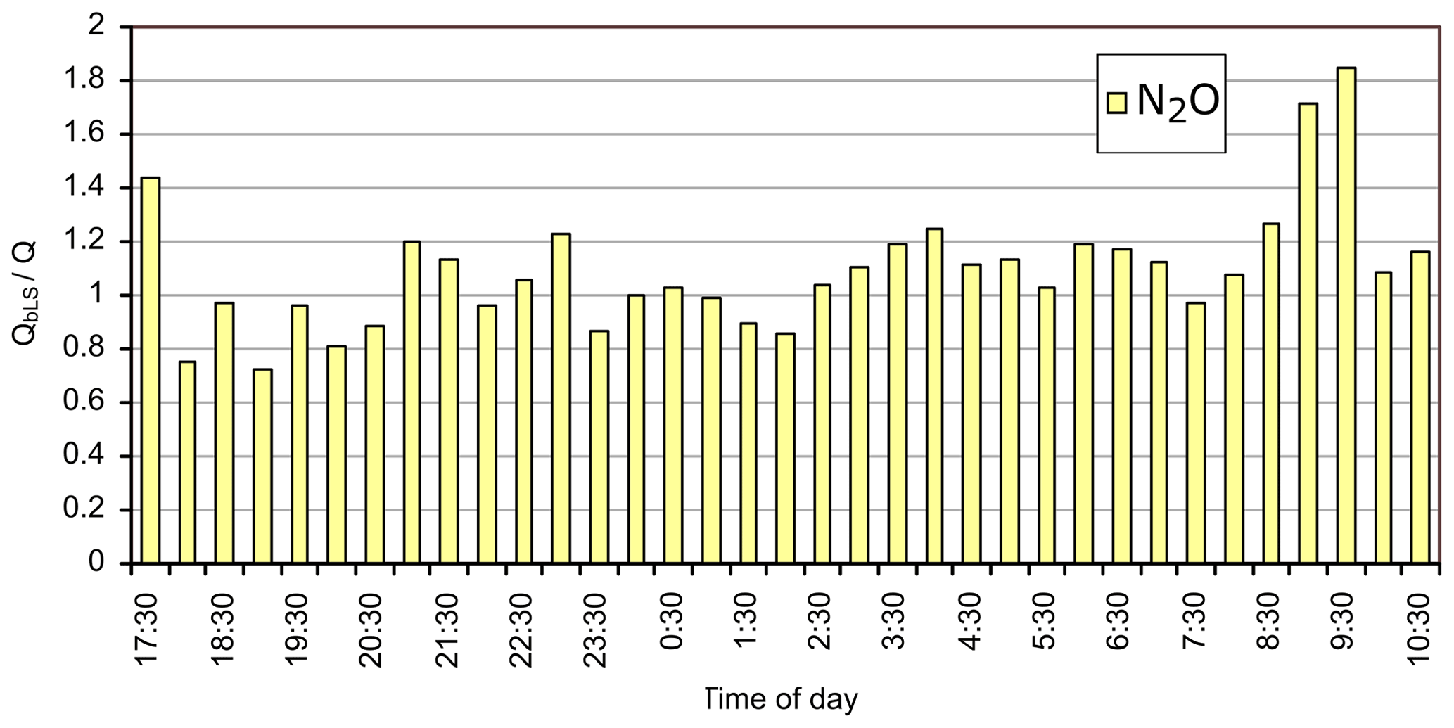
Figure A2Ratio of calculated (QbLS) to known N2O (Q) fluxes for the ground-level 40×25 m grid source (source 4), using OP-FTIR mole fractions and measurement path 2.
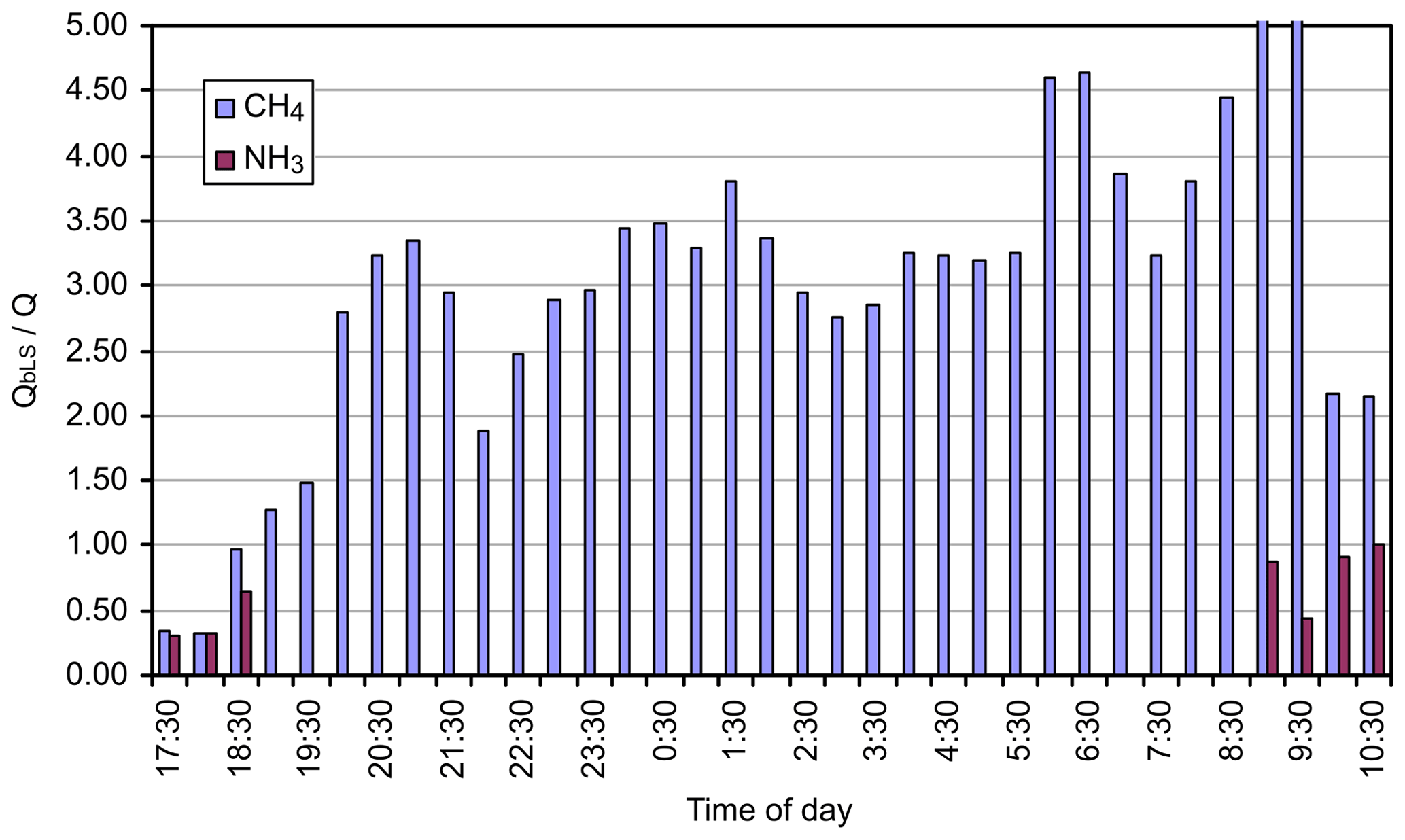
Figure A3Ratio of calculated (QbLS) to known CH4 and NH3 (Q) fluxes for the ground-level 40×25 m grid source (source 4), using OP-FTIR mole fractions and measurement path 2.
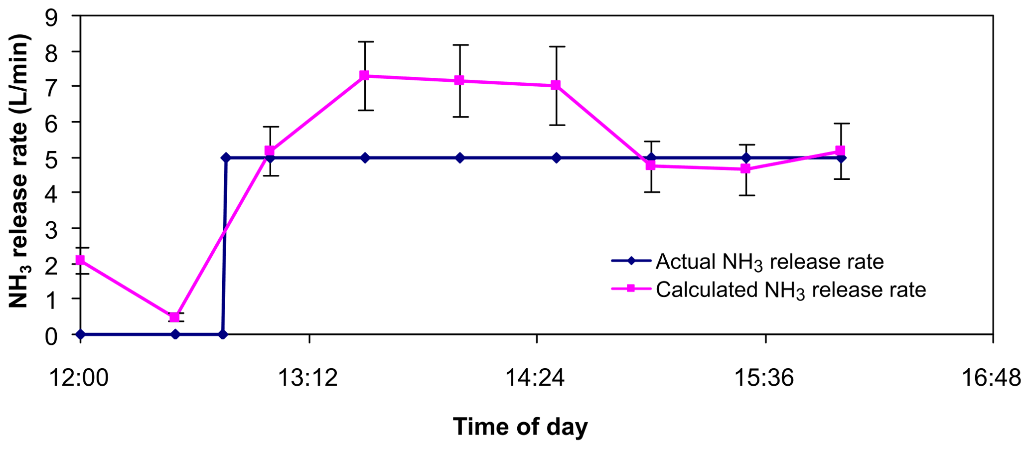
Figure A4Controlled release from 25×25 m grid (source 3). The calculated release was the average of bLs WindTrax calculations using line-averaged mole fraction measurements from two NH3 lasers.
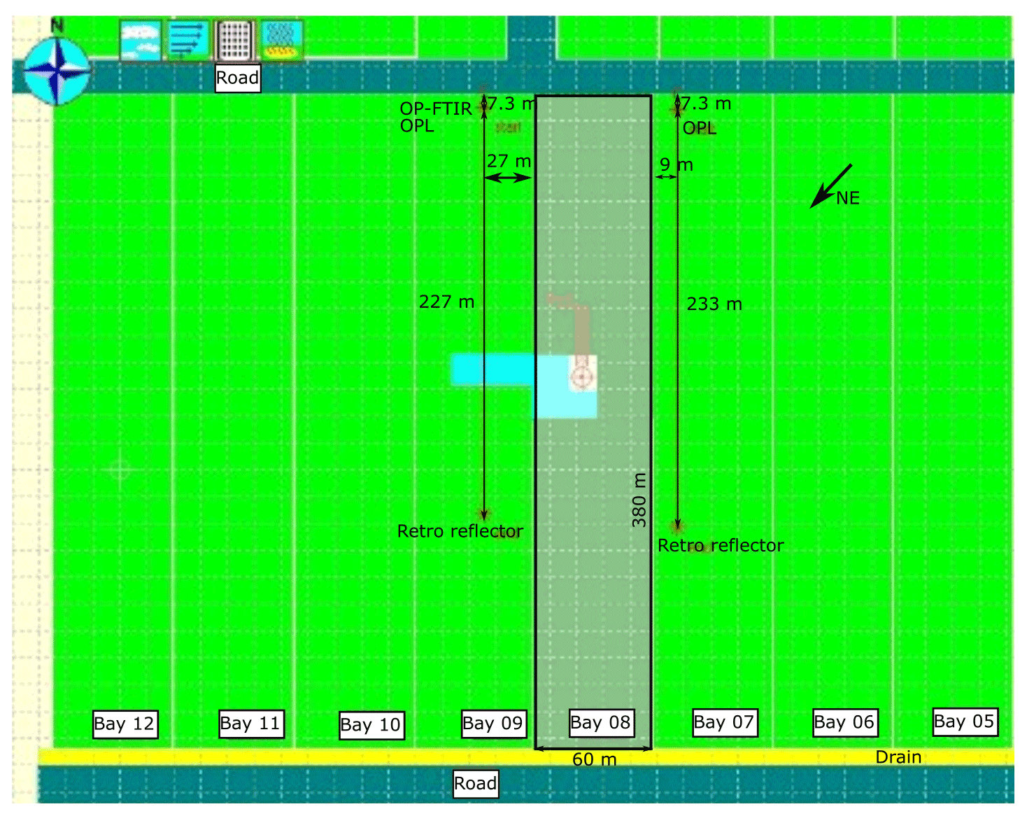
Figure A5A WindTrax map showing the layout of herd emissions studied at Kyabram on 21 March 2006.
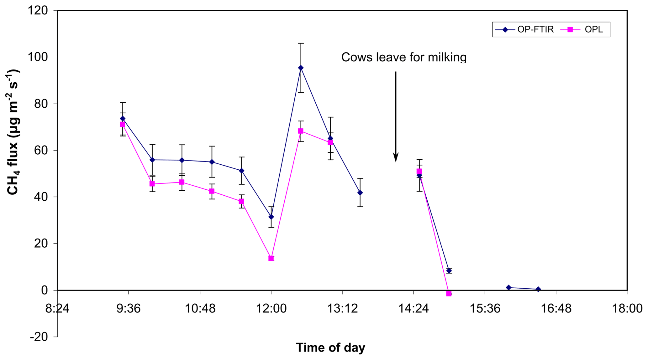
Figure A6CH4 fluxes determined from OP-FTIR and OPL (1012) data and the bLs model at Kyabram on 21 March 2006.

Figure A7NH3 fluxes determined from OP-FTIR data and the bLs model in WindTrax at Kyabram on 21 March 2006.
The raw data are not available to the public. For any inquiry about the data, please contact the corresponding author (mei.bai@unimelb.edu.au).
All authors contributed to conceptualization, methodologies, field measurements, data analysis, and original draft preparation. MB, DG, CPW, ZL, and SM contributed to final draft. DC, OTD, RE, DG, and RE contributed to funding acquisition and investigation.
The contact author has declared that neither they nor their co-authors have any competing interests.
Publisher’s note: Copernicus Publications remains neutral with regard to jurisdictional claims in published maps and institutional affiliations.
We wish to acknowledge the assistance of many: Ron Teo from the University of Melbourne, as well as the Victorian Kyabram research station for access to their laboratory and experimental facilities, for provision of micrometeorological data at Kyabram, and for the assistance of their staff, particularly Kevin Kelly and Rob Baigent. We wish to thank also the Australian Greenhouse Office for their encouragement. The authors would like to thank Travis Naylor and Graham Kettlewell from the University of Wollongong for their assistance during this study.
This research has been supported by the ACT Government (grant no. 0054-0405-Chen).
This paper was edited by Reem Hannun and reviewed by two anonymous referees.
Bai, M.: Methane emissions from livestock measured by novel spectroscopic techniques, Doctor of Philosophy PhD thesis, School of Chemistry, University of Wollongong, University of Wollongong, NSW, Australia, 303 pp., 2010.
Bai, M., Flesch, T., McGinn, S., and Chen, D.: A snapshot of greenhouse gas emissions from a cattle feedlot, J. Environ. Qual., 44, 1974–1978, https://doi.org/10.2134/jeq2015.06.0278, 2015.
Bai, M., Sun, J., Dassanayake, K. B., Benvenutti, M. A., Hill, J., Denmead, O. T., Flesch, K. T., and Chen, D.: Non-interference measurement of CH4, N2O and NH3 emissions from cattle, Anim. Prod. Sci., 56, 1496–1503, https://doi.org/10.1071/AN14992, 2016.
Bai, M., Flesch, K. T., Trouvé, R., Coates, T. W., Butterly, C., Bhatta, B., Hill, J., and Chen, D.: Gas Emissions during Cattle Manure Composting and Stockpiling, J. Environ. Qual., 49, 228–235, https://doi.org/10.1002/jeq2.20029, 2020.
Bjorneberg, L. D., Leytem, B. A., Westermann, T. D., Griffiths, R. P., Shao, L., and Pollard, J. M.: Measurement of atmospheric ammonia, methane, and nitrous oxide at a concentrated dairy production facility in Southern Idaho using open-path FTIR Spectrometry, T. ASABE, 52, 1749–1756, https://doi.org/10.13031/2013.29137, 2009.
Bühler, M., Häni, C., Kupper, T., Ammann, C., and Brönnimann, S.: Quantification of methane emissions from waste water treatment plants, EGU General Assembly 2020, Online, 4–8 May 2020, EGU2020-13389, https://doi.org/10.5194/egusphere-egu2020-13389, 2020.
Crenna, B., Thomas, K. F., and Wilson, J. D.: WindTrax 2.0.6.8 (06 12 04). Alberta Canada, http://www.thunderbeachscientific.com/ (lase access: 30 August 2021), 2006.
Denmead, O. T.: Novel meteorological methods for measuing trace gas fluxes, Philos. T. R. Soc. A., 351, 383–396, 1995.
Denmead, O. T., Harper, L. A., Freney, J. R., Griffith, D. W. T., Leuning, R., and Sharpe, R. R.: A mass balance method for non-intrusive measurements of surface-air trace gas exchange, Atmos. Environ., 32, 3679–3688, 1998.
Denmead, O. T., Bai, M., Turner, D., Li, Y., Edis, R., and Chen, D.: Ammonia emissions from irrigated pastures on Solonetz in Victoria, Australia, Geoderma Regional, 20, e00254, https://doi.org/10.1016/j.geodrs.2020.e00254, 2020.
de Klein, C., Novoa, R. S. A., Ogle, S., Smith, K. A., Rochette, P., Wirth, T. C., McConkey, B. G., Mosier, A., and Rypdal, K.: N2O emissions from managed soils, and CO2 emissions from lime and urea application. In: 2006 IPCC Guidelines for National Greenhouse Gas Inventories Volume 4 Agriculture, Forestry and Other Land Use, edited by: Eggelston, S., Buendia, L., Miwa, K., Ngara, T., and Tanabe, K., Cambridge University Press, Cambridge, United Kingdom and New York, NY, USA, 2006.
Esler, M. B., Griffith, D. W. T., Wilson, S. R., and Steele, L. P.: Precision trace gas analysis by FT-IR Spectroscopy. 1. Simultaneous analysis of CO2, CH4, N2O, and CO in Air, Anal. Chem., 72, 206–215, https://doi.org/10.1021/ac9905625, 2000.
Feitz, A., Schroder, I., Phillips, F., Coates, T., Negandhi, K., Day, S., Luhar, A., Bhatia, S., Edwards, G., Hrabar, S., Hernandez, E., Wood, B., Naylor, T., Kennedy, M., Hamilton, M., Hatch, M., Malos, J., Kochanek, M., Reid, P., Wilson, J., Deutscher, N., Zegelin, S., Vincent, R., White, S., Ong, C., George, S., Maas, P., Towner, S., Wokker, N., and Griffith, D.: The Ginninderra CH4 and CO2 release experiment: An evaluation of gas detection and quantification techniques, Int. J. Greenh. Gas Con., 70, 202–224, https://doi.org/10.1016/j.ijggc.2017.11.018, 2018.
Flesch, T. K., Wilson, J. D., and Yee, E.: Backward-time Lagrangian stochastic dispersion models and their application to estimate gaseous emissions, J. Appl. Meteorol. Clim., 34, 1320–1332, https://doi.org/10.1175/1520-0450(1995)034<1320:BTLSDM>2.0.CO;2, 1995.
Flesch, T. K., Wilson, J. D., Harper, L. A., Crenna, B. P., and Sharpe, R. R.: Deducing ground-to-air emissions from observed trace gas mole fractions: A field trial, J. Appl. Meteorol. Clim., 43, 487–502, https://doi.org/10.1175/1520-0450(2004)043<0487:DGEFOT>2.0.CO;2, 2004.
Flesch, T. K., Desjardins, R. L., and Worth, D.: Fugitive methane emissions from an agricultural biodigester, Biomass Bioenerg., 35, 3927–3935, https://doi.org/10.1016/j.biombioe.2011.06.009, 2011.
Flesch, T. K., Vergé, X. P. C., Desjardins, R. L., and Worth, D.: Methane emissions from a swine manure tank in western Canada, Can. J. Anim. Sci., 93, 159–169, https://doi.org/10.4141/cjas2012-072, 2012.
Flesch, T. K., Baron, V., Wilson, J., Griffith, D. W. T., Basarab, J., and Carlson, P.: Agricultural gas emissions during the spring thaw: Applying a new measuremnt technique, Agr. Forest Meteorol., 221, 111–121, https://doi.org/10.1016/j.agrformet.2016.02.010, 2016.
Griffith, D. W. T.: Synthetic calibration and quantitative analysis of gas-phase FT-IR spectra, Appl. Spectrosc., 50, 59–70, 1996.
Griffith, D. W. T., Deutscher, N. M., Caldow, C., Kettlewell, G., Riggenbach, M., and Hammer, S.: A Fourier transform infrared trace gas and isotope analyser for atmospheric applications, Atmos. Meas. Tech., 5, 2481–2498, https://doi.org/10.5194/amt-5-2481-2012, 2012.
Harper, L. A., Flesch, T. K., Powell, J. M., Coblentz, W. K., Jokela, W. E., and Martin, N. P.: Ammonia emissions from dairy production in Wisconsin, J. Dairy Sci., 92, 2326–2337, https://doi.org/10.3168/jds.2008-1753, 2009.
Harper, L. A., Flesch, T. K., and Wilson, J. D.: Ammonia emissions from broiler production in the San Joaquin Valley1, Poultry Sci., 89, 1802–1814, https://doi.org/10.3382/ps.2010-00718, 2010.
IPCC: Emissions from managed soils, and CO2 emissions from lime and urea application, in: 2006 IPCC Guidelines for National Greenhouse Gas Inventories. Vol. 4. Agriculture forestry and other land use, Ch. 11, Prepared by the National Greenhouse Gas Inventories Programme, International Panel on Climate Change, Hayama, Japan, 54 pp., 2006.
Laubach, J., Barthel, M., Fraser, A., Hunt, J. E., and Griffith, D. W. T.: Combining two complementary micrometeorological methods to measure CH4 and N2O fluxes over pasture, Biogeosciences, 13, 1309–1327, https://doi.org/10.5194/bg-13-1309-2016, 2016.
Loh, Z., Chen, D., Bai, M., Naylor, T., Griffith, D., Hill, J., Denmead, T., McGinn, S., and Edis, R.: Measurement of greenhouse gas emissions from Australian feedlot beef production using open-path spectroscopy and atmospheric dispersion modelling, Aust. J. Exp. Agr., 48, 244–247, 2008.
Loh, Z., Leuning, R., Zegelin, S., Etheridge, D., Bai, M., Naylor, T., and Griffith, D.: Testing Lagrangian atmospheric dispersion modelling to monitor CO2 and CH4 leakage from geosequestration, Atmos. Environ., 43, 2602–2611, 2009.
McGinn, S. M.: Measuring greenhouse gas emissions from point sources, Can. J. Soil Sci., 86, 355–371, 2006.
McGinn, S. M. and Flesch, T. K.: Ammonia and greenhouse gas emissions at beef cattle feedlots in Alberta Canada, Agr. Forest Meteorol., 258, 43–49, https://doi.org/10.1016/j.agrformet.2018.01.024, 2018.
McGinn, S. M., Flesch, T. K., Harper, L. A., and Beauchemin, K. A.: An Approach for Measuring Methane Emissions from Whole Farms, J. Environ. Qual., 35, 14–20, https://doi.org/10.2134/jeq2005.0250, 2006.
McGinn, S. M., Coates, T., Flesch, T. K., and Crenna, B.: Ammonia emission from dairy cow manure stored in a lagoon over summer, Can. J. Soil Sci., 88, 611–615, https://doi.org/10.4141/CJSS08002, 2008.
NIR: National Inventory Report 2015, Volume 1, Commonwealth of Australia 2017, https://www.awe.gov.au/, last access: 20 June 2017.
Paton-Walsh, C., Smith, T. E. L., Young, E. L., Griffith, D. W. T., and Guérette, É.-A.: New emission factors for Australian vegetation fires measured using open-path Fourier transform infrared spectroscopy – Part 1: Methods and Australian temperate forest fires, Atmos. Chem. Phys., 14, 11313–11333, https://doi.org/10.5194/acp-14-11313-2014, 2014.
Phillips, F. A., Naylor, T., Forehead, H., Griffith, D. W. T., Kirkwood, J., and Paton-Walsh, C.: Vehicle Ammonia Emissions Measured in An Urban Environment in Sydney, Australia, Using Open Path Fourier Transform Infra-Red Spectroscopy, Atmosphere, 10, 208, https://doi.org/10.3390/atmos10040208, 2019.
Rothman, L. S., Jacquemart, D., Barbe, A., Chris Benner, D., Birk, M., Brown, L. R., Carleer, M. R., Chackerian Jr, C., Chance, K., Coudert, L. H., Dana, V., Devi, V. M., Flaud, J. M., Gamache, R. R., Goldman, A., Hartmann, J. M., Jucks, K. W., Maki, A. G., Mandin, J. Y., Massie, S. T., Orphal, J., Perrin, A., Rinsland, C. P., Smith, M. A. H., Tennyson, J., Tolchenov, R. N., Toth, R. A., Vander Auwera, J., Varanasi, P., and Wagner, G.: The HITRAN 2004 molecular spectroscopic database, J. Quant. Spectrosc. Ra., 96, 139–204, https://doi.org/10.1016/j.jqsrt.2004.10.008, 2005.
Rothman, L. S., Gordon, I. E., Barbe, A., Benner, D. C., Bernath, P. F., Birk, M., Boudon, V., Brown, L. R., Campargue, A., Champion, J. P., Chance, K., Coudert, L. H., Dana, V., Devi, V. M., Fally, S., Flaud, J. M., Gamache, R. R., Goldman, A., Jacquemart, D., Kleiner, I., Lacome, N., Lafferty, W. J., Mandin, J. Y., Massie, S. T., Mikhailenko, S. N., Miller, C. E., Moazzen-Ahmadi, N., Naumenko, O. V., Nikitin, A. V., Orphal, J., Perevalov, V. I., Perrin, A., Predoi-Cross, A., Rinsland, C. P., Rotger, M., Šimečková, M., Smith, M. A. H., Sung, K., Tashkun, S. A., Tennyson, J., Toth, R. A., Vandaele, A. C., and Vander Auwera, J.: The HITRAN 2008 molecular spectroscopic database, J. Quant. Spectrosc. Ra., 110, 533–572, https://doi.org/10.1016/j.jqsrt.2009.02.013, 2009.
Smith, P., Bustamante, M., Ahammad, H., Clark, H., Dong, H., Elsiddig, E. A., Haberl, H., Harper, R., House, J., Jafari, M., Masera, O., Mbow, C., Ravindranath, N. H., Rice, C. W., Abad, C. R., Romanovskaya, A., Sperling, F., and Tubiello, F.: Agriculture, Forestry and Other Land Use (AFOLU), in: Climate Change 2014: Mitigation of Climate Change. Contribution of Working Group III to the Fifth Assessment Report of the Intergovernmental Panel on Climate Change, edited by: Edenhofer, O., Pichs-Madruga, R., Sokona, Y., Farahani, E., Kadner, S., Seyboth, K., Adler, A., Baum, I., Brunner, S., Eickemeier, P., Kriemann, B., Savolainen, J., Schlömer, S., von Stechow, C., Zwickel, T., and Minx, J. C., Cambridge University Press, Cambridge, United Kingdom and New York, NY, USA, 2014.
Smith, T. E. L., Wooster, M. J., Tattaris, M., and Griffith, D. W. T.: Absolute accuracy and sensitivity analysis of OP-FTIR retrievals of CO2, CH4 and CO over concentrations representative of “clean air” and “polluted plumes”, Atmos. Meas. Tech., 4, 97–116, https://doi.org/10.5194/amt-4-97-2011, 2011.
Tomkins, N. W., McGinn, S. M., Turner, D. A., and Charmley, E.: Comparison of open-circuit respiration chambers with a micrometeorological method for determining methane emissions from beef cattle grazing a tropical pasture, Anim. Feed Sci. Tech., 166–167, 240–247, https://doi.org/10.1016/j.anifeedsci.2011.04.014, 2011.
Tonini, M.: Measuring methane emissions from cattle using an open path FTIR tracer based method, Bachelor of Science with Honours, Department of Chemistry, University of Wollongong, Wollongong, Australia, 68 pp., 2005.
VanderZaag, A. C., Flesch, T. K., Desjardins, R. L., Baldé, H., and Wright, T.: Measuring methane emissions from two dairy farms: Seasonal and manure-management effects, Agr. Forest Meteorol., 194, 259–267, https://doi.org/10.1016/j.agrformet.2014.02.003, 2014.
The laser CH4 mole fractions may be less than those determined by FTIR because the latter's path was only 5 m downwind of the source, while the laser path was 8 m downwind. The reverse situation possibly applies to the NH3 measurements, in which the NH3 laser path was 3 m upwind of that of the FTIR (Fig. 2).