the Creative Commons Attribution 4.0 License.
the Creative Commons Attribution 4.0 License.
 | 17 Jun 2022
Horizontal geometry of trade wind cumuli – aircraft observations from a shortwave infrared imager versus a radar profiler
Henning Dorff
Heike Konow
Felix Ament
This study elaborates on how aircraft-based horizontal geometries of trade wind cumulus clouds differ whether a one-dimensional (1D) profiler or a two-dimensional (2D) imager is used. While nadir profiling devices are limited to a 1D realization of the cloud transect size, with limited representativeness of horizontal cloud extension, 2D imagers enhance our perspectives by mapping the horizontal cloud field. Both require high resolutions to detect the lower end of the cloud size spectrum.
In this regard, the payload aboard the HALO (High Altitude and LOng Range Research Aircraft) achieves a comparison and also a synergy of both measurement systems. Using the NARVAL II (Next-Generation Aircraft Remote-Sensing for Validation Studies) campaign, we combine HALO observations from a 35.2 GHz cloud and precipitation radar (1D) and from the hyperspectral 2D imager specMACS (Munich Aerosol Cloud Scanner), with a 30 times higher along-track resolution, and compare their cloud masks. We examine cloud size distributions in terms of sensitivity to sample size, resolution and the considered field of view (2D or 1D). This specifies impacts on horizontal cloud sizes derived from the across-track perspective of the high-resolution imager in comparison to the radar curtain. We assess whether and how the trade wind field amplifies uncertainties in cloud geometry observations along 1D transects through directional cloud elongation.
Our findings reveal that each additional dimension, no matter of the device, causes a significant increase in observed clouds. The across-track field yields the highest increase in the cloud sample. The radar encounters difficulties in characterizing the trade wind cumuli size distribution. More than 60 % of clouds are subgrid scale for the radar. The radar has issues in the representation of clouds shorter than 200 m, as they are either unresolved or are incorrectly displayed as single grid points. Very shallow clouds can also remain unresolved due to too low radar sensitivity. Both facts deteriorate the cloud size distribution significantly at this scale. Double power law characteristics in the imager-based cloud size distribution do not occur in radar observations. Along-track measurements do not necessarily cover the predominant cloud extent and inferred geometries' lack of representativeness. Trade wind cumuli show horizontal patterns similar to ellipses, with a mean aspect ratio of 3:2 and having tendencies of stronger elongation with increasing cloud size. Instead of circular cloud shape estimations based on the 1D transect, elliptic fits maintain the cloud area size distribution. Increasing wind speed tends to stretch clouds more and tilts them into the wind field, which makes transect measurements more representative along this axis.
- Article
(6571 KB) - Full-text XML
- BibTeX
- EndNote


Marine shallow cumulus clouds exhibit the highest frequency of occurrence in the trade wind region (Brueck et al., 2015; Bony et al., 2017) and affect climate up to global scale (Siebesma, 1998; Wing and Emanuel, 2014). Nevertheless, these clouds are only partially understood (Vial et al., 2017; Nuijens and Siebesma, 2019). According to general circulation models (GCMs), they drive the largest spread in cloud feedbacks (Medeiros et al., 2015; Ceppi et al., 2017). Not only the trends in cloud cover, which change the Earth's radiation budget (Rieck et al., 2012; Nuijens et al., 2015; Bony et al., 2015) but also horizontal radiative transport through the cloud edges are crucial (Zinner et al., 2006; Hinkelman et al., 2007). Nuijens and Siebesma (2019) review an underestimation in the coupling of cloud properties and the boundary layer (BL) regarding cloud geometries, organization, trade winds (e.g. Bretherton and Blossey, 2017; Tompkins and Semie, 2017; Stevens et al., 2019b), and precipitation (Vogel et al., 2016). To grow our knowledge of cloud controlling factors (CCFs) and their role in climate change (Siebesma et al., 2009; Klein et al., 2017), the macrophysics, i.e. cloud geometries, have to be sampled together with predominant BL conditions.
Due to the omnipresence of trade wind cumuli over the tropical oceans, their observation requires remote sensing. Vertical profilers, such as on CloudSat (Stephens et al., 2002), can measure overpassed clouds in vertical transects (Illingworth et al., 2007). However, since profilers characterize cloud properties in a one-dimensional (1D) way, moving space-/airborne platforms require long-distance paths so that they are of limited use for local cloud cover estimates (Astin et al., 2001). Fixed locations, e.g. supersites like the Barbados Cloud Observatory (BCO), furnish ground-based cloud profiling downstream the trade winds (Stevens et al., 2016). They need several hours of cloud passage until the cloud cover variance decreases (Klingebiel et al., 2021). Both 1D methods estimate cloud properties outside transects statistically or outside assumptions of circular cloud shapes (van de Poll et al., 2006; Romps and Vogelmann, 2017), which constrains the utility for model verification (Winker et al., 2017).
Vertically pointing cloud imagers observe clouds in the two-dimensional (2D) horizontal plane. In addition to enlarging the field of observation, 2D imagers are better equipped to address the challenge of trade wind cumuli showing sizes ranging across several orders of magnitude (Zhao and Girolamo, 2007; Wood and Field, 2011; Mieslinger et al., 2019), as they can resolve properties of trade wind cumuli down to decametre scale (Zhao and Girolamo, 2007). Clouds having a subgrid scale for a common hectometre profiler resolution may have extensive unresolved radiative impacts or be misinterpreted by erroneous cloud size distributions and unresolved horizontal cloud properties. In a large spaceborne framework of shallow cloud properties, Mieslinger et al. (2019) bridge the gap between horizontal cloud geometries and trade wind BL conditions from reanalyses. However, most spaceborne imagers are inadequate for detecting sharp water vapour gradients (Chazette et al., 2014) or distinguishing between overlapping clouds.
A synergy of along-track cloud profiling that captures their 2D horizontal structure at high resolution, while measuring BL conditions simultaneously, is rarely provided. Yet, the payload of the High Altitude and LOng Range Research Aircraft (HALO) fulfils such requirements (Stevens et al., 2019a). The Next-Generation Aircraft Remote-Sensing for Validation Studies (NARVAL) II was the first campaign over the tropical Atlantic, where the 2D imager specMACS (Munich Aerosol Cloud Scanner; Ewald et al., 2016) was mounted in a nadir perspective aboard HALO and complemented the profiling observations based on radar and lidar. Therefore, we elucidate the capabilities of such modern airborne remote sensing in characterizing horizontal geometries of shallow trade wind cumuli. In this context, the imager resolution, which is high against the radar, receives detailed attention as large eddy simulations (LESs) become capable of capturing cloud properties at a hectometre scale for large domains over 100 km (Stevens et al., 2020). We investigate (i) what remains unresolved in statistics of horizontal trade wind cumulus geometries using radar profiler with hectometre along-track resolution. The emerging cloud size distributions that include decametre scale feed our modelling understanding.
Profilers' restriction to 1D transects may lead to sampling uncertainties for airborne cloud statistics (e.g. Gutleben et al., 2019), whereas the imager detects the horizontal 2D cloud field. We evaluate how airborne 2D imagers enhance our perspectives on cloud geometries compared to 1D profiling. Similar to LES studies (Barron et al., 2020), which aim to transfer from 1D cloud lengths to 2D horizontal sizes, we assess the following questions: (ii) how representative are cloud sizes derived from 1D transects after considering a nadir 2D field of view (FOV), and (iii) which simplified shape approximates the horizontal cloud projections? Since Mieslinger et al. (2019) identified trade winds as the most powerful CCF, we further infer (iv) to what extent strong trade winds and corresponding cloud elongation play a role in the assessment of horizontal cloud sizes using transect measurements.
Pursuing these four questions, our paper is structured as follows: Sect. 2 specifies the used cloud detection products from HALO, namely the radar and imager cloud masks. Periods ensuring colocated observations are identified. Section 3 encompasses our applied synergy of both cloud masks comprising FOV adaptation between both devices and coordinate transformation in order to gain cloud geometries in the horizontal plane. Section 4 addresses the first two research questions, viewing on the suitability of radar transects to characterize horizontal trade wind cumuli size distributions. This section also searches for simplified shapes that approximate horizontal cloud projections. For application, Sect. 5 is dedicated to wind-induced impacts on horizontal cloud elongation and their relevance when using transect measurements. The conclusions consider the abilities of a prospective flight campaign to answer the research questions emerging from this study.
We analyse observations from the research aircraft HALO, which is characterized by a high cruising level and long range (Krautstrunk and Giez, 2012). HALO is equipped with several remote sensing devices measuring in different spectral ranges (Stevens et al., 2019a). Our comparison of trade wind cumuli geometries from airborne profiler and imager concentrates on a 1D profiling cloud and precipitation radar and a hyperspectral imager enabling the determination of horizontal cloud geometries in a 2D image. This section depicts both devices and their cloud masks being used. Periods of colocated observations are given.
2.1 Cloud and precipitation radar
Aboard HALO, the cloud and precipitation radar MIRA-35 (manufactured by METEK GmbH) is mounted in a downward-pointing configuration. MIRA-35 is a monostatic, pulsed, and magnetron Ka-band Doppler radar operating in 35.2 GHz within the water vapour window (Ewald et al., 2019). The output in a sampling rate of 1 Hz mainly comprises the radar reflectivity, Doppler velocity, spectral width, and linear depolarization ratio. Raw measurements are provided in a vertical resolution of 28.8 m. For typical cruising levels at 13 km and a typical aircraft speed around 200 m s−1, the radar sensitivity is about −30 dBZ, whereby the footprint size at the surface is about 130 m. By infiltrating clouds, the profiling radar enables the observation of vertical cloud structures and represents a fundamental component of airborne cloud analysis. Clouds are resolved at roughly 200 m in the along-track. Together with the HALO Microwave Package (Mech et al., 2014), the processed data are provided in a unified grid with a vertical resolution of 30 m and a time resolution of 1 Hz (Konow et al., 2018, 2019).
2.2 Hyperspectral imager
The hyperspectral imager specMACS (Ewald et al., 2016) was developed at the Meteorological Institute at the Ludwig Maximilian University (LMU) of Munich, with the goal to detect clouds and aerosol optical properties, as well as aerosol tracers. This is done using two passive hyperspectral cameras which measure the incoming solar radiation within the 400–2500 nm wavelength spectrum. One camera measures radiances in the visible and near-infrared spectrum (VNIR; 400–1000 nm). The second camera measures within the shortwave infrared (SWIR) spectrum in the range of 1000–2500 nm (Ewald et al., 2016). Both cameras are line-scanning slit spectrometers that capture radiances in two dimensions. When the aircraft overpasses a certain domain, the downward-pointing cameras look on clouds in the along-track and across-track perspective from above. This results in a 2D observation field. For the purpose of this study, we focus on the cloud products gained from the SWIR camera, which allows more explicit cloud masking under the presence of sunglint. This camera measures incoming radiation in 320 across-track pixels and in 256 wavelengths and enables the observation of the across-track cloud top in a FOV of 35.5∘.
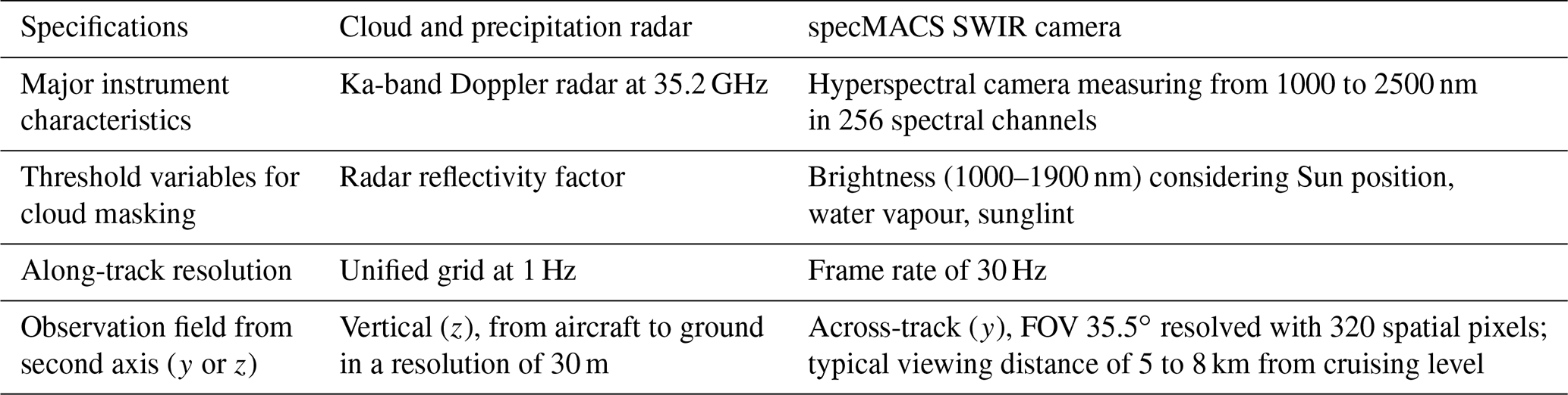
2.3 Cloud masks
For the cloud geometry analysis, the cloud masks from the radar (Sect. 2.1) and imager (Sect. 2.2) are prerequisite. Their different measurement principles result in individual cloud mask specifications (Table 1). The radar cloud mask is also provided on the unified grid (Sect. 2.1) and derived from the measured radar reflectivity following the methods of the BCO radar cloud mask algorithm (Konow, 2020). Since reflectivity values were already filtered, i.e. adjusted for constant background noise, the remaining detected signals represent clouds and precipitation. As soon as a radar signal exceeds the radar sensitivity, the pixel is assigned as cloud (value of 1) or, otherwise, clear. Measurement gaps were interpolated and the clouds were morphologically closed. Clouds being measured very close to each other (1 s, which represents around 200 m) are connected.
To identify clouds from the imager, the intuitive approach of brightness thresholds does not yield unambiguous results, as various processes affect the radiance values of each pixel. These are mainly the brightness dependency on the Sun's position, atmospheric water vapour, and the presence of sunglint, meaning that there is the reflection of sunlight at the ocean surface under specific conditions. Sunglint-contaminated pixels can have higher radiance values than cloud pixels. Hence, the imager cloud mask is a best estimate of a water-vapour-adapted brightness mask, together with a simulated sunglint mask, based on Tsang et al. (1985). In contrast to the 1 Hz radar cloud mask, the imager cloud mask has an along-track resolution based on a frame rate of 30 Hz. This cloud mask was developed by Gödde (2018) and is accessible on the macsServer (Gödde and Kölling, 2018).
Besides the along-track axis, both cloud masks provide a second dimension. While the radar mask considers the vertical profile in a 30 m resolution, the imager mask represents the 2D horizontal cloud field seen from above. For a typical cruising altitude of 10 km, the FOV of specMACS corresponds to an across-track viewing distance of about 6.4 km. With a frame rate of 30 Hz, the spatial resolution of the imager cloud mask results in roughly 18 m along and 38 m across the flight track at this altitude.
Table 1Cloud mask specifications from radar and imager specMACS (SWIR camera).
2.4 Synchronous cloud observations during NARVAL II
To compare horizontal trade wind cumuli geometries from an airborne profiler and imager, we use observations from the NARVAL II campaign, conducted in August 2016 at the edge of the Intertropical Convergence Zone (ITCZ) east of Barbados under the influence of the North Atlantic trade winds (Stevens et al., 2019a). For that, overlapping measurements from radar and imager are indispensable. In total, 10 research flights (RFs) were performed in shallow and deep convection (Konow et al., 2019). However, we had to exclude three flights without reliable radar operation and the first transfer flight (RF01), as measurements were mostly taken north of the tropics (>20∘ N). The remaining flights suffer from some interruptions in reliable overlapping cloud observations (Fig. 1) due to the window freezing in front of the imager at high cruising levels that prevented reliable cloud detection and other occurring disturbances due to issues at the radar and its calibration (Ewald et al., 2019).
Around half of the duration of the remaining RFs provide suitable, colocated measurements. In total, this corresponds to more than 24 flight hours. Circle flight patterns were mainly performed to examine large-scale divergence in Bony and Stevens (2019), wherein dropsondes (Busen, 2012) captured the vertical atmospheric state. We make use of these sonde profiles in Sect. 5 to characterize the trade wind field in the vicinity of shallow convection and to relate the winds to the geometries of embedded cumulus clouds. This analysis substantially benefits from frequent sonde releases during RF03 and RF06 (Fig. 1).
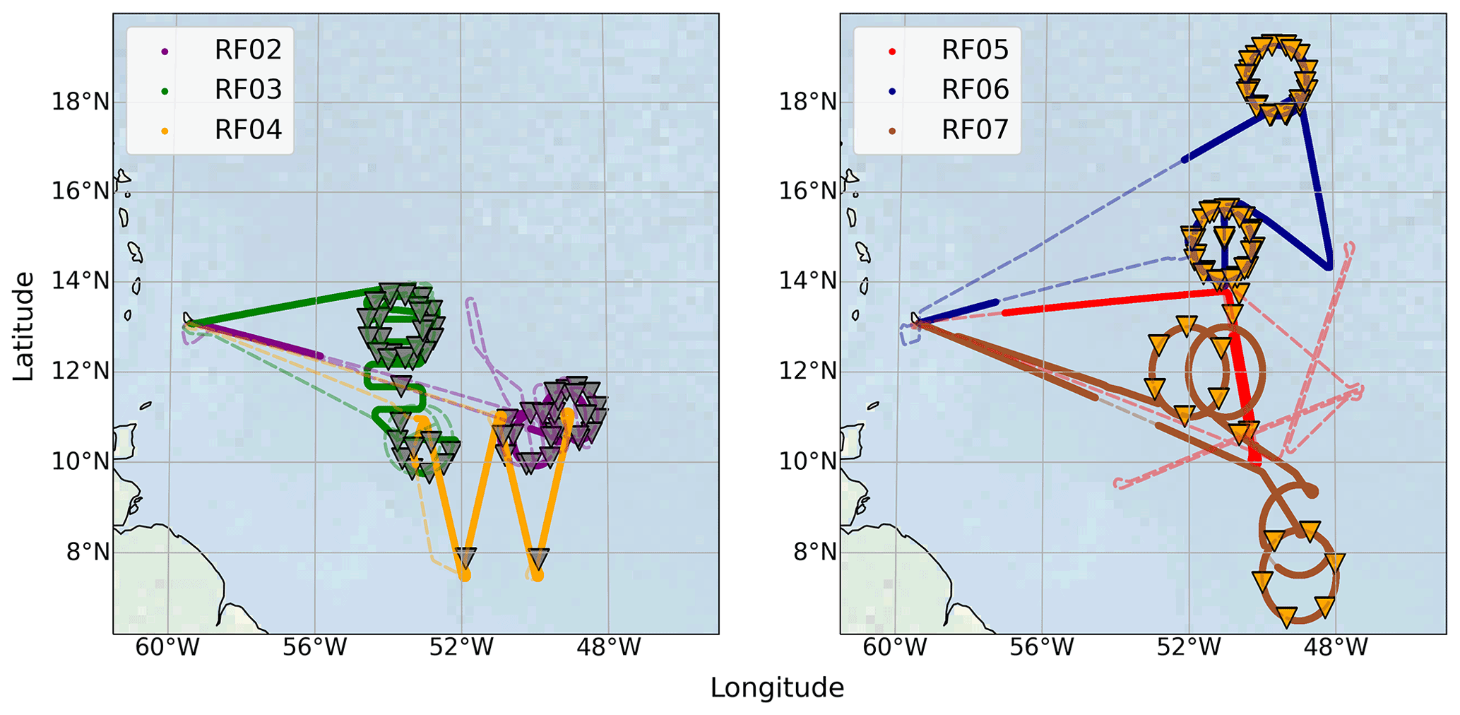
Figure 1Considered flight tracks from NARVAL II (dashed lines) that provide observations of tropical clouds from the radar and imager specMACS. Periods in which both devices (radar and imager) were operating reliably and simultaneously are highlighted as bold lines. Dropsonde releases less than 15 min away from overlapping measurements of radar and imager are indicated as triangles. Background map was made with Natural Earth.
While Gutleben et al. (2019) examined lidar-based cloud properties from NARVAL II under the influence of Saharan dust, this study complements the statistics more generally under aspects of differences in radar profiler and imager perspective and their resolution. For the derivation of single cloud geometries and inter-device comparison, the different viewing directions of both cloud masks have to be contemplated. While 1D along-track cloud geometries can be inferred immediately from the time axis, when considering the cruising speed, the imager across-track axis is initially given in camera pixels and has to be transformed to distance-based coordinates if 2D geometries are desired. The major steps for both requirements are specified.
3.1 Viewing direction and cloud object identification
When comparing both devices in their overlapping transect, one has to consider that the central imager across-track pixel is shifted 0.55∘ to the left in the flight direction referred to the radar. Moreover, the imager FOV is 2.6∘ ahead of the radar, so both devices look at identical clouds at different time frames. This time shift depends on the cloud-top height (CTH); the lower and more distant the clouds are from the aircraft, the more the detection times deviate between the devices. This leads to non-negligible time offsets for cloud detection. Following the methods in Höppler et al. (2020), offsets are calculated using the CTH, which we obtain from the radar. The offsets are determined from the aircraft distance to the clouds and the aircraft speed and subsequently applied to the radar cloud mask. The same clouds are hence referenced to equivalent time frames in both devices.
Single clouds are identified as coherent objects by a connected component analysis, where each cloud pixel is connected with its neighbour cloud pixel (Fig. 2). According to the 2D eight-connectivity algorithm (Rosenfeld and Kak, 1982), we consider neighbouring cloud pixels as being coherent when they are connected at one of their edges or corners. Each cloud is assigned an identification number (ID). By comparing the radar reflectivity with the cloud IDs (Fig. 2a, b), the morphological closing applied to the cloud mask becomes visible. For the along-track axis during the given scene, it is already notable that the imager (Fig. 2c, d) counts many more clouds than the radar. This worthwhile remark is discussed in more detail in Sect. 4.
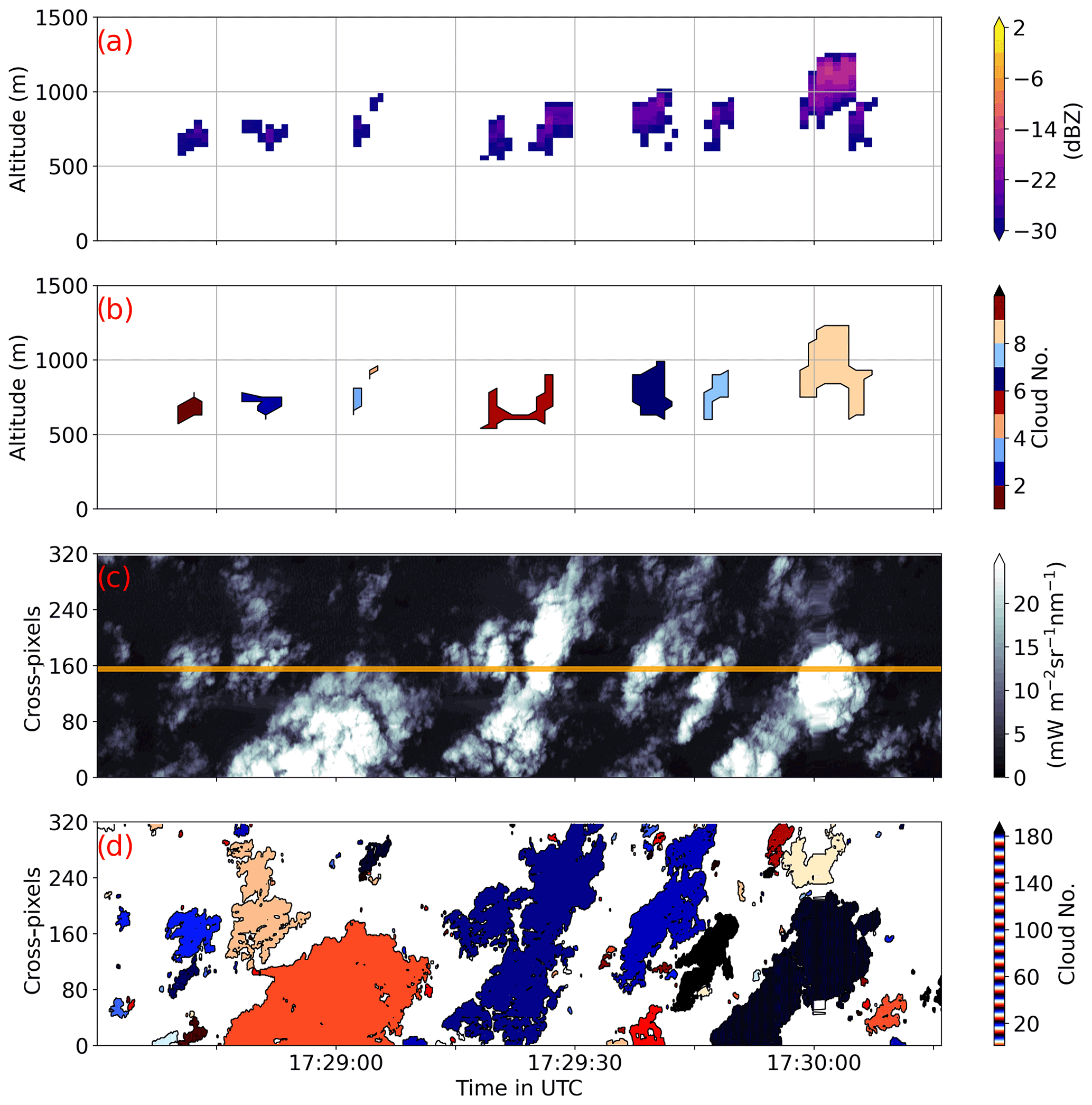
Figure 2Cloud scene during RF02 from 17:28:30 to 17:30:15 UTC, vertically magnified from the radar (a, b) and as seen from specMACS (c, d). For each device, the upper panel shows the measurements of the cloud scene, namely the reflectivity factor in decibels relative to Z (dBZ; radar) and radiances given in milliwatts per square metre, per steradian, and per nanometre (mW m−2 sr−1 nm−1) of the 1600 nm channel from the SWIR camera (imager specMACS). Each imager cross-track pixel has a FOV of 0.22∘. The yellow curtain in panel (c) represents the radar FOV. Each lower panel indicates the number of clouds based on their IDs obtained from the connected component analysis applied to the cloud masks of the radar (b) and imager (d), respectively.
3.2 The two-dimensional distance-based pixels
To characterize 2D cloud geometries in the horizontal projected plane, and not only along-track specific, each cloud object has to be transformed into a local distance-based coordinate system (Fig. 3). For that, the transformation takes into account the coordinate frame of the SWIR camera CSWIR where across-track pixels have fixed viewing directions in reference to HALO. Since the geometric field covered by a single imager pixel depends on the flight attitude, the initial coordinate frame CSWIR is aligned differently at each time frame. To transform the direction vectors from CSWIR into the target coordinate system, rotation matrices, which include the flight attitude (i.e. pitch, yaw, and roll angle), yield the pixel viewing directions in the local reference system and provide both axes in metres. Dividing the vertical distance between the camera at cruising level zCamera and radar-based CTH, given with an accuracy of 30 m, results in the slanted distance d that specifies the stretching factor for the vector projection down to the CTH layer zCTH. Tracking downwards along d, cloud pixels are referenced to metres. The projection causes cloud sizes to primarily depend on the distance to the CTH. When analysing 2D cloud geometries, the following aspects need to be considered:
-
The discrete along-track CTH values are interpolated in time and synchronized to the imager resolution to achieve a continuous along-track representation of CTH.
-
When observing very thin low-level clouds from very high cruising levels above 10 km, due to too low sensitivity, the radar partly tends to underestimate CTH or, in some cases, does not detect a cloud in contrast to the imager in the overlapping FOV. Arising too low a CTH can affect the interpolation and lead to erroneous continuous CTH representation. Therefore, a quality check includes the lifting condensation level (LCL), calculated and interpolated in time from the dropsonde profiles, as a threshold approximation for minimum CTH. CTH values below the LCL are replaced.
-
The across-track cloud observation by the imager requires CTH estimates that are also outside of the radar transect. As a simplified assumption, the derived CTH is set constant in the across-track direction.
-
In order to mitigate the projection issues for across-track clouds, CTH uncertainties are limited by only considering shallow convection regimes with lower CTH variability. This restriction is also advantageous regarding sources of errors stemming from the imager viewing geometry. The further away clouds are located at the edges of the FOV, the larger the pixel viewing zenith angle and the more clouds are actually detected from the side. In contrast, if clouds are shallower and lower, they are less observed from the side (Henderson-Sellers and McGuffie, 1990).
-
As uncertainties of CTH, mainly in the across-track direction, prevail in a certain amount even in shallow convection, we use the along-track variability of CTH as an estimate of spatial CTH uncertainty to be included in the projection.
-
Periods that the radar identifies with a high amount of multi-level and vertically overlapping clouds are excluded, as the imager cloud mask does not account for different height levels and merges these clouds.
-
Clouds extending out of the FOV are neglected as their 2D geometries exterior of the FOV are not obtainable. In addition, we exclude clouds having an along-track cloud size bigger than the imager across-track FOV, as large clouds orientated along the flight course would be considered preferentially otherwise. Since cloud size then becomes artificially limited by the FOV size, cloud size statistics remain biased for undersampled larger clouds approaching the typical image scale.
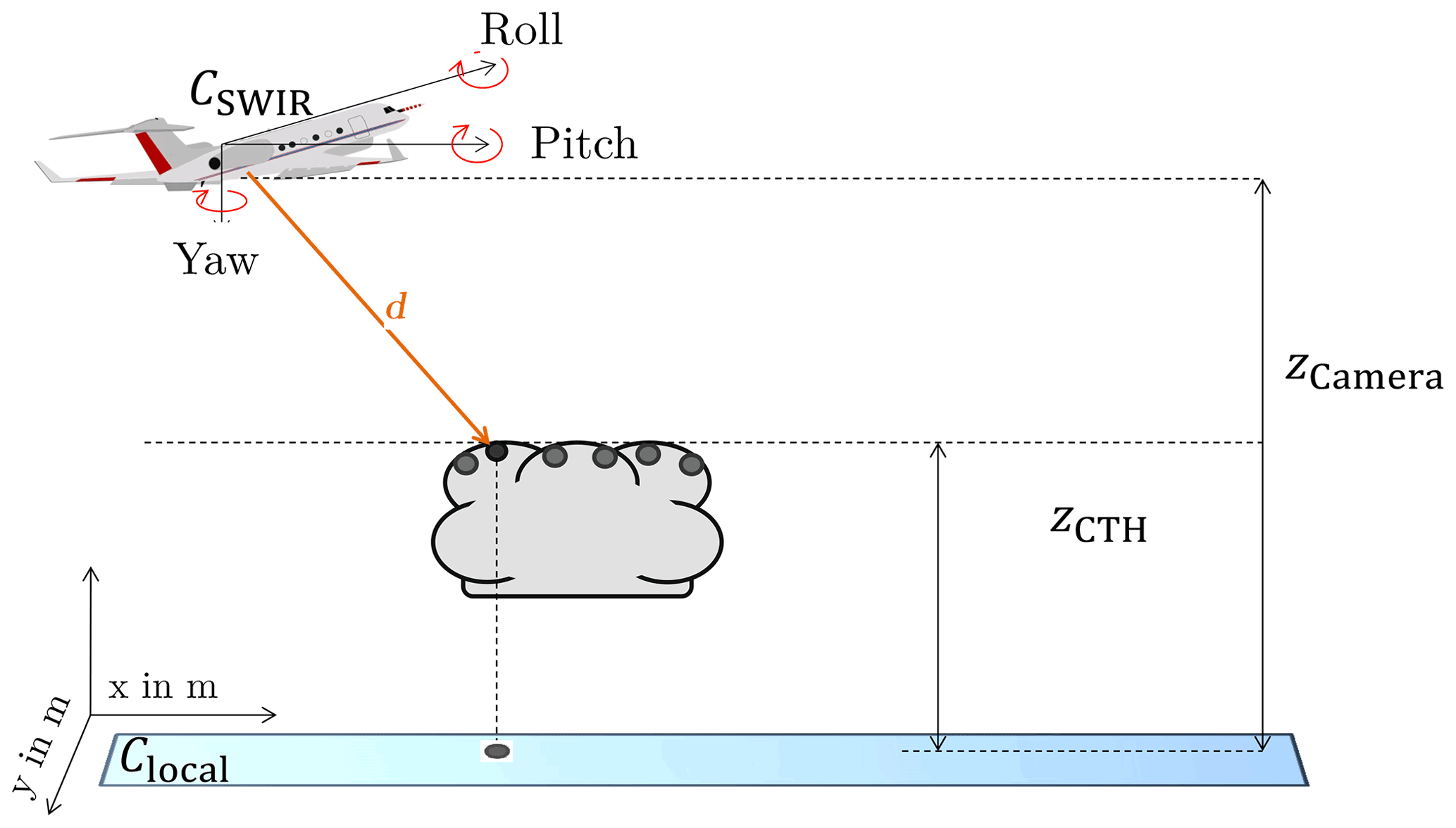
Figure 3Illustration of the transformation from cloud pixels in the camera coordinate system CSWIR into the local distance-based reference system. Aircraft yaw, pitch, and roll axes are defined in the top left-hand corner.
3.3 Regridded imager cloud mask
To specify resolution impacts on cloud geometry statistics separately from the impact of the FOV (1D and 2D), a coarse-gridded imager cloud mask mimics the spatiotemporal radar resolution with a time resolution of 1 Hz and a larger footprint for each pixel, while still considering the across-track FOV. The resulting mean cloud cover below 0.5 inside the coarse-gridded pixels are labelled as clear and vice versa if above. The emerging cloud mask is shown in Fig. 4 for an exemplary scene. This coarsening constitutes a conceptional simplification, as the sensitivities are by no means trivial and idealized in this regridded mask.
3.4 Cloud size distribution
Among cloud geometries, cloud size distributions are of fundamental interest. The vast majority of trade wind cumuli are rather small, while the size distribution tails off towards rare larger clouds. Covering decametres up to several 10 km, their size distributions are conventionally analysed in logarithmic mode. Satellite observations found that trade wind cumuli size distributions obey a power law distribution (e.g. Sengupta et al., 1990; Benner and Curry, 1998; Zhao and Girolamo, 2007; Mieslinger et al., 2019). The frequency n(D) of the cloud size D, being the area-equivalent diameter, is described as follows:
with the slope β<0 and α being a parameter. In logarithmic mode, β can be obtained by a linear least square fit. Due to strong decay in frequency with increasing cloud size, Mieslinger et al. (2019) recommend adopting exponentially increasing bin widths, designated as logarithmic bins. The transformation to logarithmic bins n(log (D)) increases the slope value by 1 to the following:
Analysing the distribution with logarithmic binning, the fitted cloud size distribution becomes less sensitive to bin size. Bin widths that are exponentially increasing allow the full range of the distribution to be considered. The size bins of cloud frequency are equidistantly displayed, and the underlying area thus represents the integral over the probability density. Also, cloud area size distributions can be approximated by (double) power law distributions (Mieslinger et al., 2019). The estimation of 2D cloud sizes from 1D chord measurements as done for the nadir space-/airborne profiler is, however, challenging and a current state of research. Simplified cloud shapes facilitate statistical estimates for the 2D size (Romps and Vogelmann, 2017).
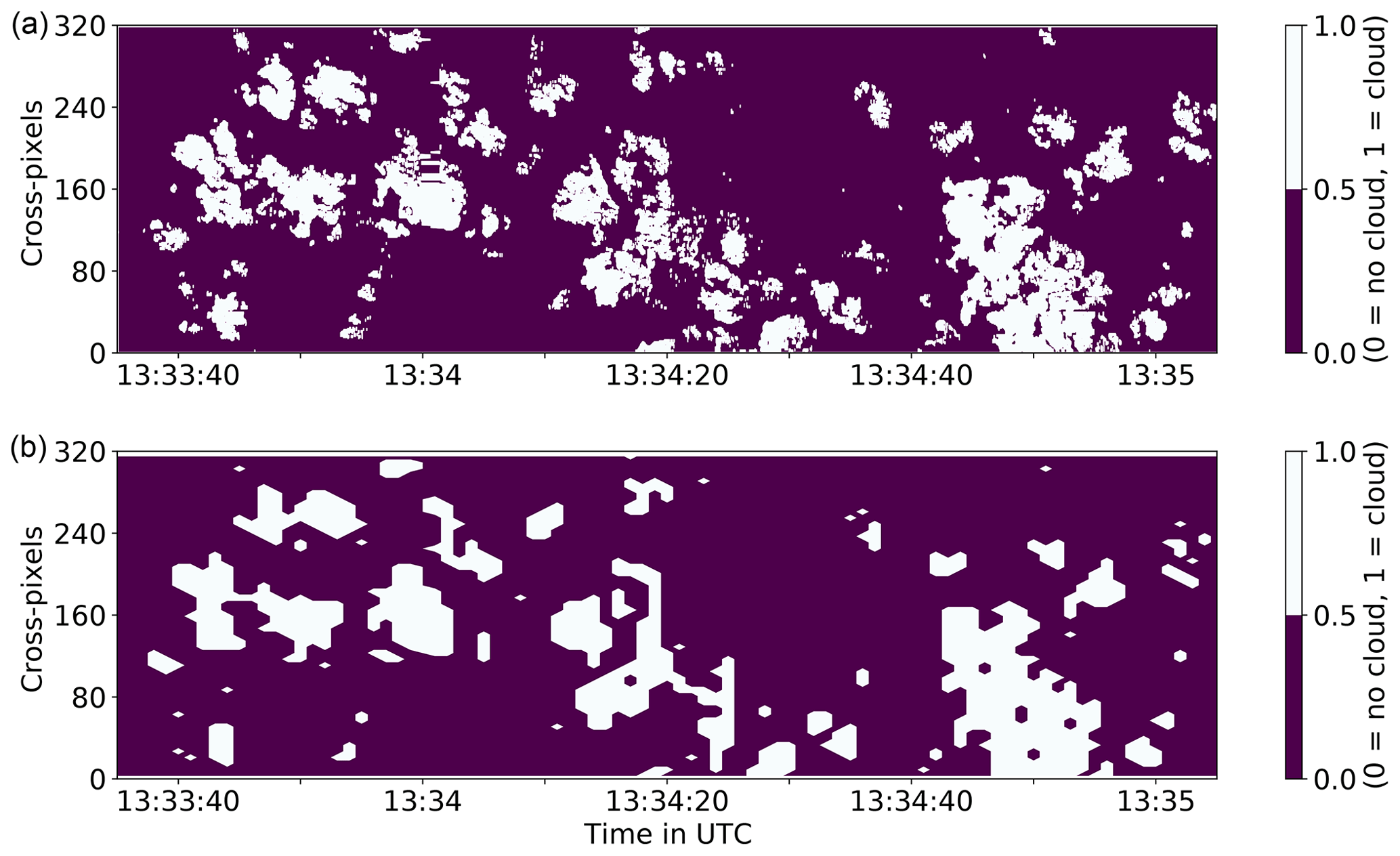
Figure 4Imager cloud mask (specMACS) of shallow cumuli from RF07 in a standard (a) and coarse-regridded resolution (b). Each imager across-track pixel has a FOV of 0.22∘.
Several studies identified double power law characteristics as the frequency decay intensifies abruptly above a certain cloud size. The interception of both fits is referred to as a scale break, for example, in Sengupta et al. (1990) and Zhao and Girolamo (2007). Mechanisms affecting its location are broadly discussed in current research. Some scientists claim that scale breaks are related to physical phenomena such as dynamical processes from interactions with the BL (Sengupta et al., 1990; Mieslinger et al., 2019). Others argue that scale breaks originate artificially and result from undersampling (Heus and Seifert, 2013).
The desired framework allows the statistical derivation of relevant cloud geometries. Using the radar and imager cloud masks, we compare 1D along-track cloud sizes with the 2D cloud extension and assess the impacts of 2D airborne observations. This comparison is based on impacts on the overall cloud size distribution in logarithmic binning according to Eq. (2). Applying logarithmic binning, we elucidate the presence of a scale break from airborne observations during NARVAL II. First, we compare the along-track cloud sizes gained from the radar with those from the 2D horizontal imager FOV given at a higher resolution. As long as we remain in the aircraft following the coordinate frame that is considering along-track cloud lengths, no restriction in cloud cutting, as suggested in Sect. 3.2, is performed in order to include a high amount of clouds. Nonetheless, we only show distributions for lengths up to 10 km because we are limited by the imager FOV when considering 2D cloud shapes. As a second step, we elaborate on the representativeness of these along-track lengths for overall cloud area statistics. Horizontal cloud areas are inferred from the 2D imager cloud mask by referring to the distance-based local coordinate frame (Sect. 3.2). Applying the Shoelace formula (Braden, 1986), we calculate cloud areas via a polygonal approach. Moreover, we reproduce the cloud area distribution by simplified cloud shapes.
Varying sensor sensitivities and resolutions change cloud masks, for example, by the contribution of small clouds (Zhao and Girolamo, 2006; Koren et al., 2008 and Fig. 4). As found in Stevens et al. (2019a), this affects along-track cloud fraction aboard HALO. Comparing the cloud fraction from regridded imager and radar after the FOV adjustment (Sect. 3.1), the radar is clearly less sensitive and detects only 78 % (33 %) of all (just shallow convective) clouds. At the same time, there are hardly any clouds which are observed by the radar only. Just the morphological closing applied to the radar cloud mask may create faulty cloud pixels. This results in a small, false positive rate of 7 % (3 %) for all (shallow convective) clouds. The rates also depend on our set regridding threshold (Sect. 3.3) but to a lesser extent. Evidently, the mentioned differences in cloud fraction affect single cloud geometries. Viewing perspectives (1D and 2D) from the radar and imager also influence the horizontal cloud geometry statistics.
Using the methods of Sect. 3, this section examines what remains unresolved in horizontal cloud size distributions when using an airborne profiler with hectometre resolution. Regarding the robustness of cloud geometries from 1D transects, this section investigates to what extent cloud geometries are reliable after considering a nadir 2D FOV. We aim for simplified shapes that can be attributed to horizontal 2D patterns of trade wind cumuli.
4.1 Cloud sample size
One general drawback of airborne cloud geometry statistics is their limited number of clouds included. The sample size is affected by the cloud mask resolution and FOV. As seen in Fig. 4, regridding the imager mask to radar resolution enlarges clouds by incorporating small holes and nearby clouds. Small, distinct clouds decrease in size or even disappear. The scene is thus represented with fewer clouds and may cause different cloud size spectra. When restricted to the overlapping 1D transect of radar and imager, it is important to note that cloud objects are counted differently due to the lack of knowledge from the across-track perspective. Only a fraction of ID-labelled clouds from the 2D field reaches into the radar curtain (Fig. 5). Otherwise, cloud fragments can appear distinctively within the curtain although belonging to one cloud. Neglecting the across-track, such fragments lead to a considerably different sample (higher cloud amount) and cloud size misrepresentation.
During our synergy period (Fig. 1), strongly different cloud sample sizes between imager and radar confirm the complexity in unambiguous horizontal cloud representation (Fig. 5). Not surprisingly, the across-track perspective, which includes clouds invisible for the nadir radar curtain, leads to a considerably larger sample. The 2D imager gathered roughly 80 000 clouds, whereas the radar gathered only around 1000 over the course of the campaign. Within the overlapping 1D transect, the imager includes less than of all clouds from its 2D field. However, not only the 2D FOV but also the high along-track resolution of the imager causes a gain of more than 78 000 clouds (98 %). When considering the coarse-gridded 2D imager mask presented in Fig. 4, the number of cloud objects decreases by around 80 % for all flights. Within the 1D transect, regridding induces a decline of 65 %. Nonetheless, the number of observed clouds therein remains twice as high as that from the radar when distinct cloud fragments are considered as new clouds. This results from the fact that very small and very low clouds remain undetected for several periods due to the lower radar sensitivity. In turn, the imager lacks vertical information. To estimate its impact, the radar cloud mask is projected horizontally by declaring time frames with at least one cloudy pixel in the vertical column as cloudy overall. This vertical lack of information results in a cloud number decrease of about 33 %.
We emphasize that given percentages can solely serve as benchmarks for the robustness of cloud sampling against missing spatial dimensions and resolution. Evidently, the different considerations of coherent cloud fragments translate into different geometry statistics. This highlights the importance of multi-dimensional cloud observation and instrument redundancy. Overall, the increase in cloud number due to the 2D field outweighs that caused by the increase in resolution.
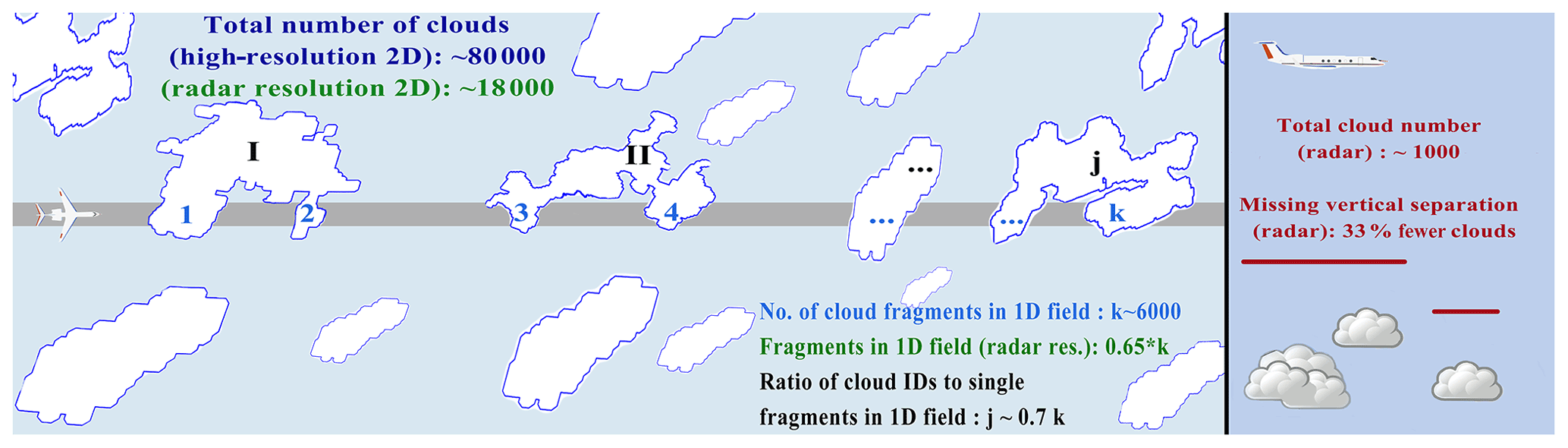
Figure 5Quantitative impact on cloud counting during NARVAL II when including the second dimension in the across-track (left) and vertical (right) for imager and radar. On the left, the roman numbers represent ID-labelled clouds reaching into the radar curtain (grey swath is not true to scale). Arabic numbers (in clouds) represent distinct cloud fragments reaching into the radar FOV. On the right, the vertical distinction between overlapping clouds shows similar increases. Numbers outside the clouds refer to the entire synergy period (specified in Sect. 3).
4.2 Impact of resolution on along-track cloud length statistics
Along-track lengths L represent the horizontal cloud sizes that can be calculated from both nadir devices directly. For both NARVAL campaigns, Gutleben et al. (2019) provide lidar-based statistics of cloud along-track lengths underneath HALO. The FOV and resolution of the lidar are thereby comparable to the radar; however, its sensitivity is not. The fact that the radar detects fewer clouds than the imager specMACS within the matching FOV (Sect. 4.1) motivates further investigation of the cloud size statistics. For this purpose, the first assessment of the impacts from colocated imager observations focusses on the intercomparison of cloud size distributions within their matching 1D FOV. This includes the regridded imager mask that mimics the radar resolution. For the relevant flight periods (Fig. 1), we can infer the robustness of the profiling curtain measurements by including cloud chord length distributions along additional parallel transects from the 2D field.
Within the overlapping FOV, the relative frequency of clouds undergoes a robust decrease with increasing cloud size for chord lengths above 500 m, no matter the resolution or device (Fig. 6). In detail, the frequency distributions deviate substantially between the devices and methods. For the cases in 1 Hz resolution (radar and regridded imager), clouds smaller than 300 m become subgrid scale due to the flight speed. Above this scale, the regridded imager and radar show similar power law distributions for cloud lengths. According to the slope parameter β (Eq. 1), the radar tends to a higher relative contribution of larger clouds in the along-track direction, leading to a weaker decay of the distribution. These deviations primarily result from different sensitivities of both devices. In particular, small trade wind clouds occur within the lowest levels and are rather thin. Although such thin clouds can be long enough to be resolved, in truth, the radar does not catch them when distances between aircraft and clouds are quite far. Another minor reason for the different slopes between the radar and regridded imager is the ability of the radar to separate clouds vertically, whereas the imager cannot distinguish between cloudy pixels from different heights and projects overlapping clouds onto a single cloud. This affects the distributions in the opposite direction, as the imager overestimates the size of these clouds. Using the imager in high resolution, the lower part of the cloud size spectrum can be resolved. While for L>500 m the slopes vary less in between both imager resolutions than in the inter-device comparison, the slope abruptly changes for cloud sizes below 500 m. The distribution thus can be described by a double power law. As determined by the least residuals (Sengupta et al., 1990), the slopes of the distributions have values of and , for smaller and larger clouds, respectively. Both fits yield an interception at around 490 m. This scale break is located slightly above the radar resolution. We discuss its location in the following when considering the entire 2D FOV with increasing cloud sample size.
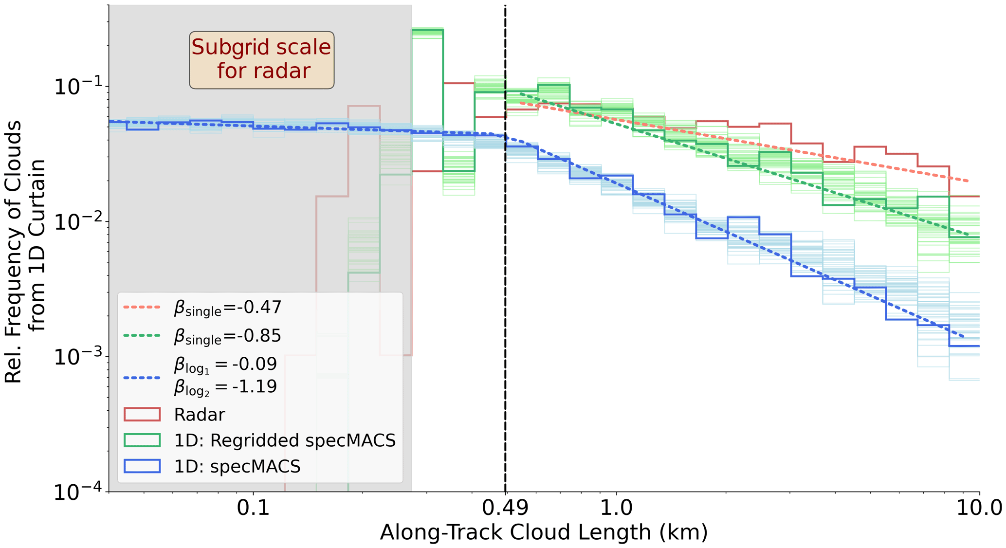
Figure 6Along-track cloud size distribution from radar and imager (specMACS) within the 1D transect of their unanimous FOV (bold). For the imager, the high resolution and regridded cloud mask (imitating radar 1 Hz resolution) are considered. Power law fits are shown as dashed lines. The vertical dashed line represents the scale break resulting from the double power law fit for the imager (blue distribution). Thin distributions illustrate cloud along-track chord lengths from successive curtains parallel to radar transect (discussed in Sect. 4.3).
4.3 Impact of the 2D FOV on along-track cloud size statistics
From now on, we extend our perspective on horizontal cloud geometries by adding the second (across-track) dimension. For instance, the relative frequency of small clouds, seen to be rather uniform in Fig. 6, is a caveat of the along-track length determination from the 1D curtain. Due to the fractal structure of clouds, it is likely that they are overpassed at one of their edges, resulting in small chord length determinations. Referred to the statistical study of Barron et al. (2020), measured chord lengths below 100 m yield little to no information about the actual cloud size distribution, as they increasingly arise from the probability of touching cloud edges. If clouds were randomly distributed in the 2D FOV, relative frequencies of their 1D chord lengths should ideally yield an equivalent distribution, regardless of the curtain chosen. From the thin distributions in Fig. 6, we note that all distribution characteristics occur more or less equivalently along other curtains parallel to the overlapping transect. Although the imager resolves decametre-scale clouds, cloud chord lengths from 1D transects merely serve as a rough guess for the distribution due to the contribution of cloud edges shifting the curves significantly towards small chord lengths (also in Fig. 2). Recorded cloud lengths can differ significantly from the actual cloud extension.
With regard to the along-track coordinate frame, the 2D perspective reveals another representation of the along-track cloud size by considering deviations in the across-track direction, which is sketched for an exemplary cloud in Fig. 7. The across-track perspective enables us to determine the maximum along-track cloud length. Although this length is an arguable size representation due to the cloud's fractal structure, it quantifies the magnitude of the maximum error when concluding from 1D cloud chord lengths of a curtain to its overall statistics and thereby decrease the erroneous representation of seemingly small chord lengths from actual cloud edges (Fig. 6). This maximum cloud size is also used by Romps and Vogelmann (2017) to approximate clouds as squares in order to transfer from 1D chord lengths to actual 2D sizes. For all imager clouds reaching into the radar curtain, we additionally calculate a mean inverse length factor defined as the average ratio of the maximum along-track length divided by effective cloud length in the radar curtain (blue and red distances in Fig. 7). This horizontal analogue to the vertical cloud overlap ratio in Sulak et al. (2020) reveals that, on average, maximum along-track cloud length differs to curtain length by a factor of around 2.63. Since this factor has a strong dependency on cloud length, its value strongly varies with cloud size and is presumably underestimated due to the FOV limits for larger clouds and is higher than its vertical analogue (Sulak et al., 2020).
Moreover, the across-track perspective includes additional cloud objects that do not reach into the radar curtain, substantially increasing cloud sample size (Sect. 4.1). Therefore, we compare the imager-based size distribution from the 1D transect in Fig. 6 with the maximum along-track cloud size distribution, including all clouds from the 2D FOV at high resolution (Fig. 8). Since 12 times the number of clouds than in the 1D curtain is involved (Sect. 4.1), the representativeness of size distributions is ensured more anyway.
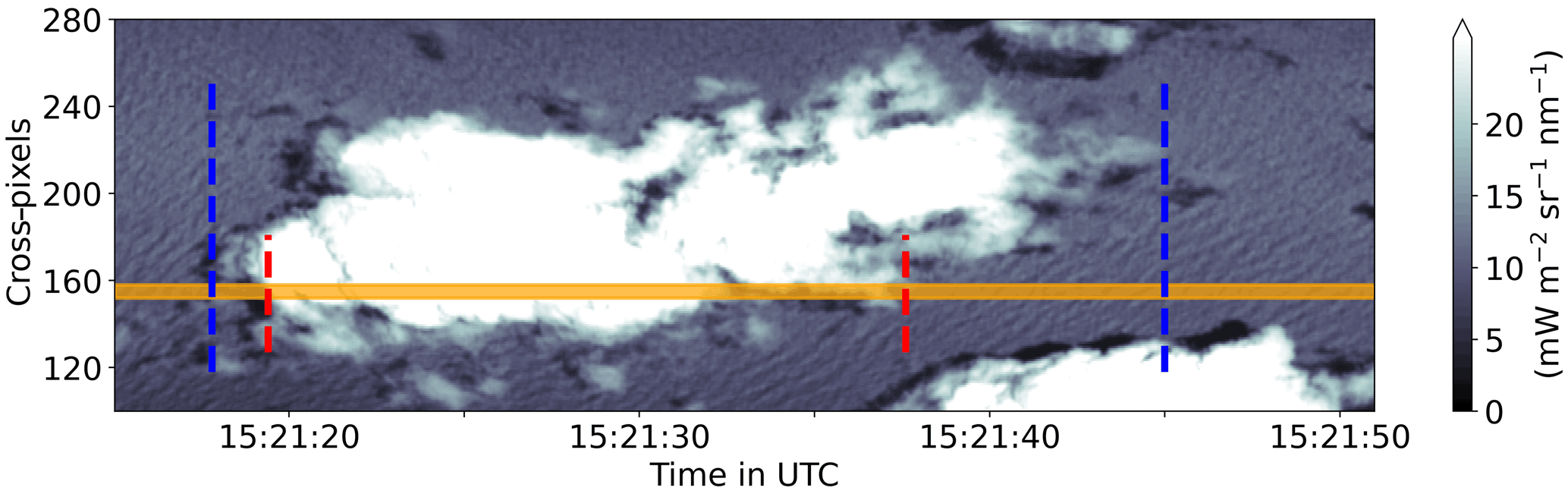
Figure 7Cloud partly reaching into the FOV of the radar (orange swath), as measured by the imager's 1600 nm channel. Dashed lines indicate the along-track cloud length within the radar FOV (red) and maximum along-track cloud length for the entire across-track extension (blue).
Concerning maximum along-track lengths, cloud sizes below 300 m, being subgrid subscale for radar resolution, represent more than 60 % of all overpassed clouds from the imager. We still observe the double power law distribution in the 2D-based sample. In addition to the resolution impact on the slope parameter β, Fig. 8 reveals that β is very sensitive to the second dimension when using the entire FOV, which is essential with regard to studies of cloud lengths obtained from 1D transects. The decay of the distribution intensifies in both size regimes. Since the across-track consideration allows the distinction between small clouds and cloud edges leading to small along-track sizes, the representation of small clouds improves by quantifying the maximum along-track length as worst-case error. Intriguingly, decametre-scale clouds occur more frequently, whereas small, medium-size clouds (L below 500 m) decrease in frequency.
Clouds outside the radar FOV increase the sample non-uniformly, which can be seen for an exemplary cloud scene in Fig. 9. When clouds are larger in the along-track axis, they generally tend to be larger in the across-track as well, often reach across-track edges covering the entire FOV, and are embedded in a cluster of numerous small clouds around. For measurements constrained on a narrow transect, this results in a lower chance of small clouds around to be captured, whereas the largest clouds (at 17:43:15 and 17:44:20 in Fig. 9) are captured anyway, regardless of the resolution and 1D transect. Transferring from 2D to 1D transects thus flattens the distribution.
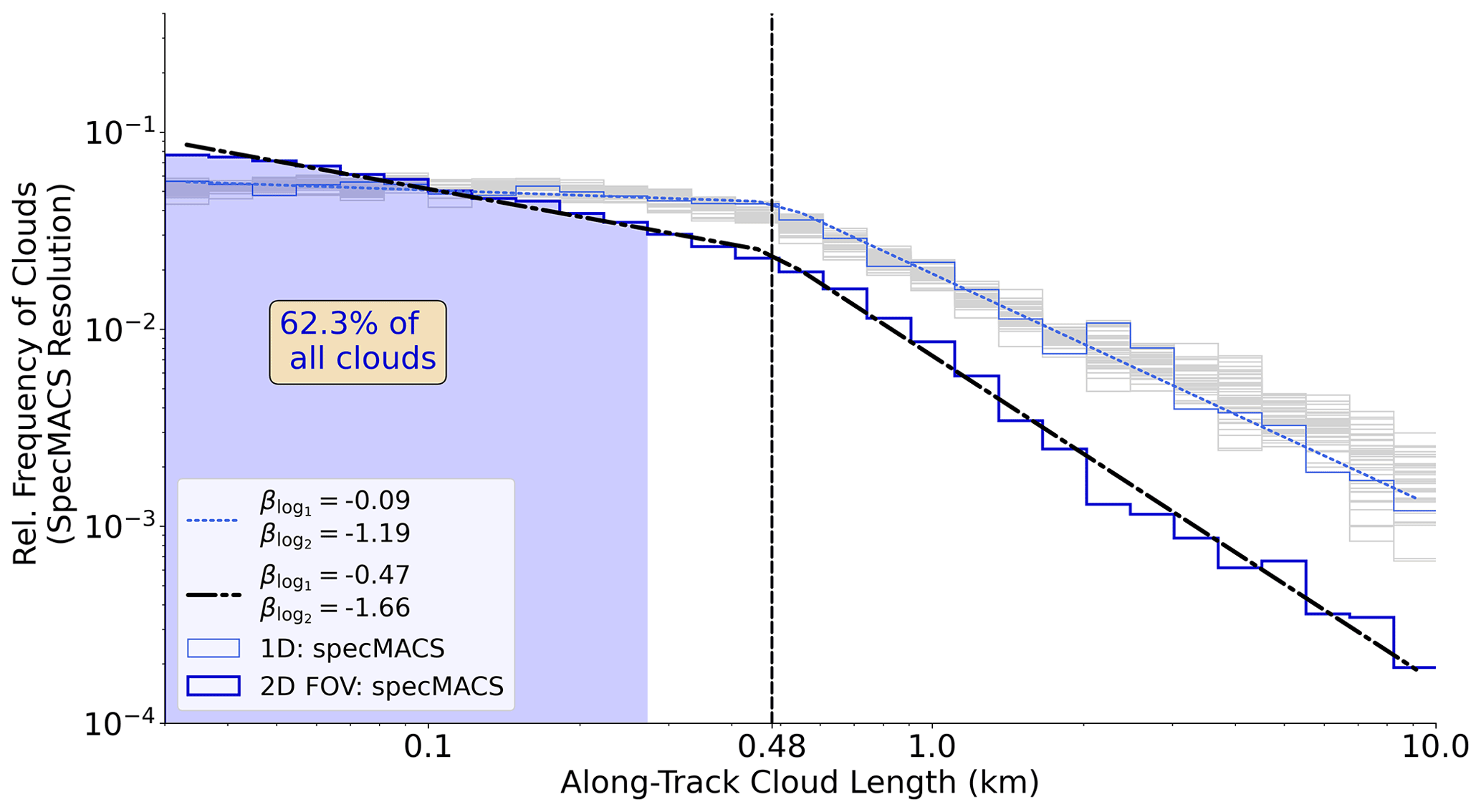
Figure 8Comparison of along-track cloud size distribution from the imager (specMACS) based on 1D transects and the 2D horizontal field. Light blue and thin grey curves are identical to the 1D-based distributions in Fig. 6. The dark distribution and fitted curve represent the distribution for the maximum along-track cloud lengths, based on the entire 2D FOV, and the vertical–dashed line shows its scale break. Shaded domains specify cloud sizes, which are unresolvable for the radar at typical flight speed.
Using the high-resolution imager, only very slight shifts in the scale break between the 2D and 1D observation field manifest. The radar resolution, however, is inadequate to resolve scale break characteristics arising from decametre-scale clouds. Both the scale break and the slope parameter correspond well to the literature values based on observations using a similar resolution, for example, Zhao and Girolamo (2007) and Mieslinger et al. (2019) or LESs (Heus and Seifert, 2013). Thus, observations from the imager specMACS during NARVAL II reproduce trade wind cloud size distributions found in comparable studies well.
Nonetheless, we highlight the ongoing debate in the literature about the location and artificial or boundary-layer-driven origin of scale breaks (Mieslinger et al., 2019). We see that resolution affects the scale break location in a way that it is missing for airborne observations in a hectometre resolution. Although Wood and Field (2011) locate scale breaks above 1 km using hectometre-scale spaceborne data, we cannot identify this from radar curtain samples. On the other hand, larger clouds may be misinterpreted from the imager if only their edges reach into the imager FOV and artificially enhance the scale break through length underestimation. If we completely neglect clouds reaching out of the FOV, we also produce biases with increasing cloud size (Sect. 3.2). Due to the complexity of the scale break origin, some studies, e.g. van Laar et al. (2019), suggest applying exponential power law fits (Ding et al., 2014). They yield single distributions and prevent the requirement of introducing a scale break.
4.4 The 2D cloud size statistics
Until this point, when identifying added values from the 2D imager, cloud sizes still referred to their 1D along-track axis. However, it is the cloud-covered area that can only be detected by the imager, and that is locally relevant for the radiation budget of the Earth (Bony et al., 2015; Brueck et al., 2015). Hence, we put now emphasis on the misrepresentation of along-track lengths for the effective 2D cloud size of all shallow cumulus clouds fully detected by the imager. The actual 1D cloud size projection, i.e. the area equivalent diameter D can considerably deviate from along-track sizes (e.g. having a value between both distances for the cloud in Fig. 7). While nadir profilers are restricted to determining along-track lengths and need to estimate cloud-covered area from circular or statistical concepts, the 2D imager allows, after the coordinate transformation (Sect. 3.2), the determination of horizontal sizes in all directions and the cloud area thereof (Sect. 3.4). Significant numbers of directional-oriented clouds may become crucial for the representativeness of profiler-based along-track size distributions. Elliptic shapes can enlighten the dominant extension and orientation of clouds which are also proven to be a typical shape at the BCO (Stevens et al., 2016; Klingebiel et al., 2021). Therefore, an elliptic fitting algorithm performed in a least square sense (Fitzgibbon et al., 1999) is applied to each fully detected cloud. To evaluate such shape simplifications and to specify limits of along-track cloud sizes, Fig. 10 depicts the cloud area distribution of the polygonal (Sect. 3.4) and elliptic approaches and compares them to circular clouds assumed from the maximum along-track extension (as in Fig. 7). From this, we classify the polygons as our reference. The statistics confine one to shallow cumulus scenarios (CTH<3 km) to limit projection errors due to CTH uncertainties (Sect. 3.2).
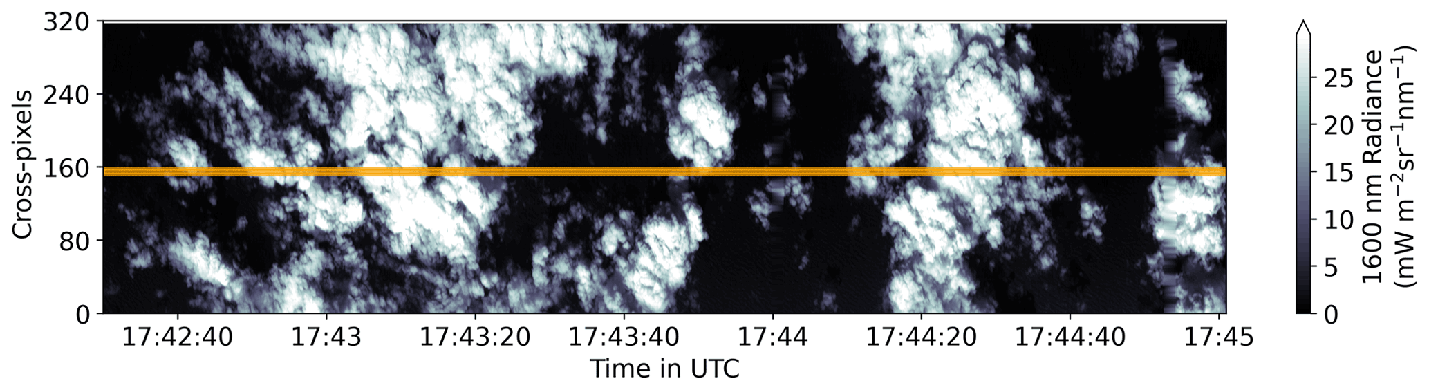
Figure 9Cloud scene containing two clouds largely extending over the entire imager FOV. Radiances from imager 1600 nm channel. The radar transect is shown in yellow.
Similar to the precedent 1D size distributions based on the 2D FOV, cloud area distributions follow double power laws (Fig. 10). Although small clouds, being subgrid scale for the radar (L<200 m), represent 80 % of all shallow clouds, they contribute to less than 7 % to the total cloud-covered area. In terms of radiation budget, the missing of most of the clouds in radar resolution is thus less severe. The polygonal and elliptic approaches reveal similar distributions. The observed trade wind cumuli have a mean aspect ratio of roughly 3:2. For each elliptic fit, we calculate the eccentricity that quantifies the elongation of clouds in an inter-comparable way. The cloud aspect ratio manifests in a mean eccentricity of 0.744. The fractal dimension δ, a metric of shape complexity relating cloud perimeter to cloud area (Lovejoy, 1982) has a relatively low value δ=1.19, indicating that trade wind cumuli shapes are rather smooth and compact (as also found in Mieslinger et al., 2019). Accordingly, we can answer our question of a realistic cloud shape simplification by the elliptic fit. Despite persisting uncertainties in CTH, mainly in the range of 50 to 300 m, the cloud area statistics are robust. After adding and subtracting the maximum CTH uncertainties (Sect. 3.2), the slopes of the distribution remain comparable.
Overall, the viewing geometry from the 2D imager has a significant impact on horizontal cloud size statistics. Circular assumptions from the along-track, instead, lead to stronger deviations in the distribution. The maximum along-track cloud length overestimates cloud sizes, and the decay of the distribution becomes weaker and is supposed to be even less when not neglecting clouds reaching out of the FOV (Sect. 3.2). Using only the radar resolution and statistical methods, e.g. considering circular assumptions (Romps and Vogelmann, 2017) or following Barron et al. (2020), such methods will fail to reproduce the actual double power laws (not shown). Cloud shapes that are rather more elliptical than circular underline the value of 2D observations by the imager. For clouds having a high eccentricity, cloud size statistics inferred from the along-track length can deviate substantially. The more strongly the clouds undergo a directional elongation, the higher the chance that along-track lengths do not consider their dominant lengths and misinterpret the horizontal extension. On the other hand, the identification of factors regulating cloud orientation can help to optimize flight segments in a way that they align with dominant cloud elongation.
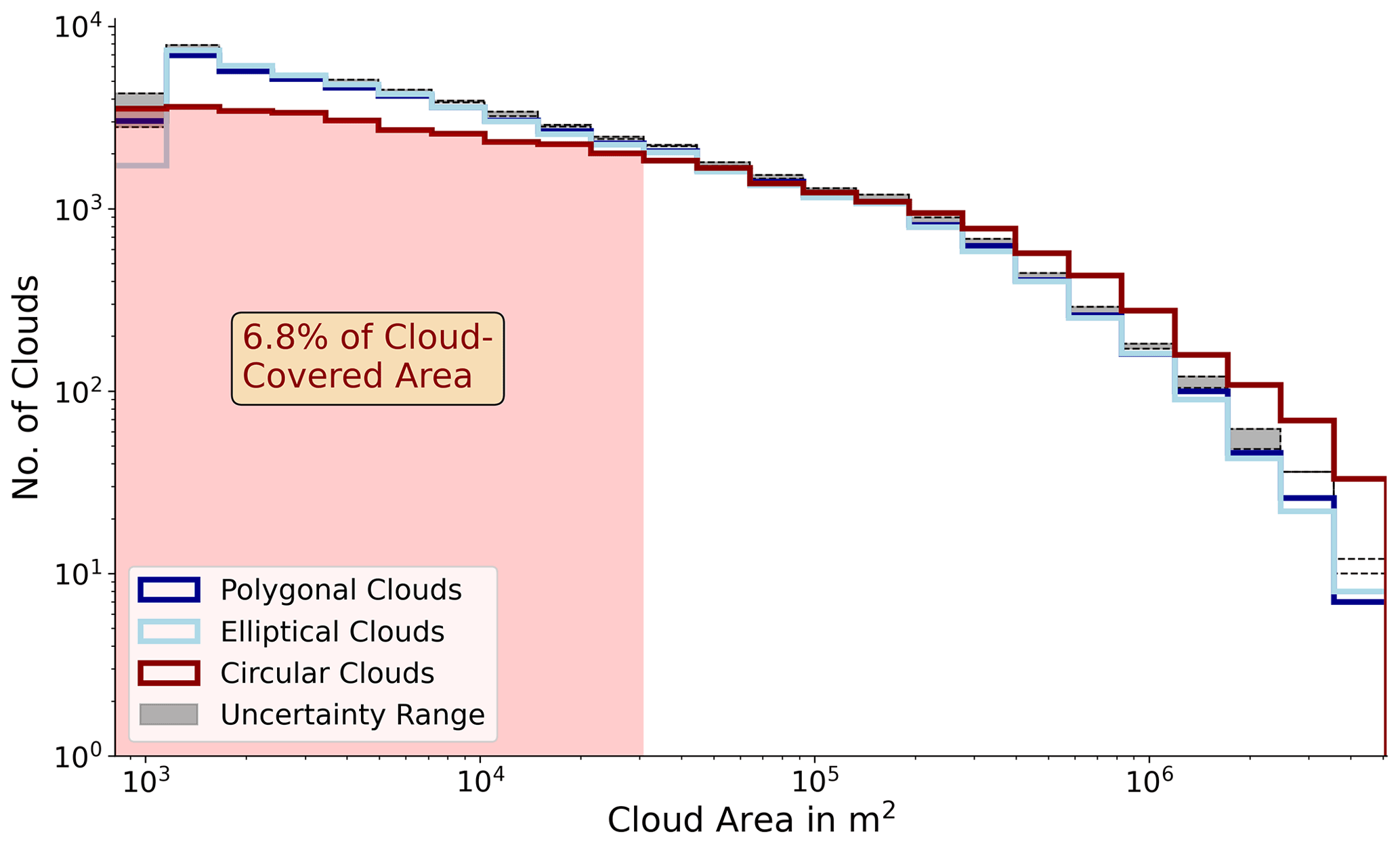
Figure 10Shallow cloud area size distribution with absolute cloud number (no.) on the y axis. The distributions of polygonal (dark blue), elliptic (light blue), and circular (dark red) clouds based on the along-track length L are compared. The red domain represents the radar subgrid scale. The grey shaded pattern illustrates the variability due to the CTH uncertainty UCTH by adding ±UCTH to each CTH.
This section refers to the elongation of clouds, where the wind field and its impact on 1D horizontal cloud geometries receives attention. In particular, trade wind cumuli driven by surface evaporation do not rise fully vertically under dominant winds with vertical wind shear. As reproduced in LES (Neggers et al., 2003; Helfer et al., 2020), this changes their horizontal projected area. Since wind speed is positively correlated to cloud deepening (Nuijens and Stevens, 2012) and to wind shear within the trade wind BL (Brueck et al., 2015), clouds can become more tilted by intensifying winds. By focusing on the cloud's elongation for our application, we investigate to what extent the trade winds play a role in measuring horizontal cloud geometries using transect measurements. Considering RF03 and RF06, 50 dropsonde releases per flight provide a high-resolution spatiotemporal representation of the vertical wind field (Fig. 1). From that, we interpolate values between the profiles in time. Focussing on shallow cumulus clouds (CTH <3000 m), the dropsondes reveal dominant easterly winds with wind speeds up to 12 m s−1 at CTH and vertical wind shear, between radar-based cloud base height (CBH) and CTH, up to 3 m s−1.
We depict the eccentricities e from the elliptic clouds (Sect. 4.2) and their frequency distributions for low and high wind speed cases at CTH in order to elaborate relations between cloud elongation and increasing wind speed (Fig. 11). Low (high) eccentricities below (above) 0.5 indicate rather circular (elliptic) clouds. By considering eccentricities for wind speed thresholds aligned to 10th and 90th percentiles, both wind cases remain clearly distinguishable in their intensity, and the respective cloud sample sizes remain of similar size. Clouds shorter than 200 m are excluded, as their elliptic fits stem from poorly resolved cloud structures. Such very small clouds would show higher eccentricities due to irregularly sized imager pixels (Sect. 2.3).
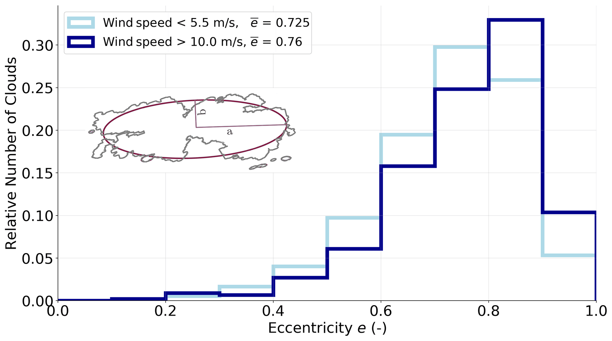
Figure 11Eccentricity distribution of shallow clouds from RF03 and RF06, showing the relative frequency of clouds in eccentricity bins, with a width of 0.1. The samples are distinguished between low (below 5.5 m s−1) and high wind speeds (above 10 m s−1) and an exemplary elliptic fit showing major (minor) semi-axis a (b) of the cloud.
We found both elliptic axes to differ by more than 10 % in length for 98 % of the clouds. Therefore, Fig. 11 shows eccentricities below 0.4 for less than 2 % of the trade wind cumuli, regardless of the strength of winds. Towards higher eccentricities, both histograms exhibit different characteristics. Stretching of clouds intensifies with increasing wind speeds. The maximum relative number of clouds is located around e=0.75 for low wind speeds and around e=0.85 for high wind speeds. At weaker winds, more clouds have eccentricities below 0.8. The mean eccentricity increases from at low wind speeds to at higher wind speeds. Around 45 % of the clouds have eccentricities higher than 0.8 in the strong wind case. If all along-track cloud observations relied on the semi-minor axis of elliptic clouds, then the mean maximum underestimations of dominant cloud lengths would be 31 % at low and 35 % at high wind speeds according to the mean eccentricity.
We hypothesize that larger clouds tilt more into the winds and become even more stretched. For the given clouds of RF03 and RF06, Fig. 12 illustrates the joint frequency distribution of eccentricity and cloud size, which also depicts both wind cases. Referring to area-equivalent cloud diameters, the cloud size distributions remain comparable between both wind cases (top panel of Fig. 12). This is in contrast to an increase in horizontal cloud size and shifts in the scale break with increasing surface wind speed, as stated in Mieslinger et al. (2019). Inspecting the contours of the joint frequency distribution, we identify an increase in eccentricity with cloud size, especially for higher wind speeds. However, since the sample size strongly decreases for larger clouds as they are rarer and more likely to extend out of the imager FOV, our hypothesis can only be proven by longer observation periods or a broader FOV. We encourage corresponding studies using, for example, ASTER as in Mieslinger et al. (2019).
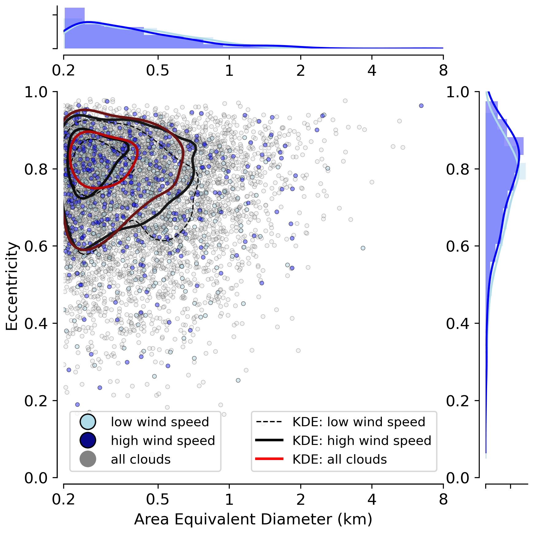
Figure 12Joint frequency distribution of cloud size (referred to as the area-equivalent diameter) and eccentricity for clouds of RF03 and RF06, with L>200 m, and the cloud samples affected by low and high wind speeds. Contour lines representing three iso-proportions of the kernel density estimate (KDE) distributions for both quantities are also given separately (top and right).
The tendency of elliptic cloud shapes raises the question of whether or not such clouds undergo predominant orientations. Since cloud stretching seems to increase under stronger winds, it is hypothesized that clouds, i.e. their observed cloud tops, tend to tilt into the prevailing wind field. If so, flight headings perpendicular to wind direction may cause underestimations in the determined cloud lengths converging the worst-case scenario, which is larger than 30 %. In both wind scenarios, the cloud lengths in wind direction yield a mean underestimation of the actual major axis length by 21.7 % for low wind speeds and by 17,2 % for high wind speeds, respectively (not shown). For 40 % of the clouds under high wind speeds and for 30 % at low wind speeds, the dominant axes are underestimated by less than 10 %, so that the wind-induced cloud orientation presumably comes into play. However, these values are ambiguous in quantifying the effective cloud orientation into the wind direction.
Therefore, we define an eccentricity adapted normalized radius r* for each cloud as follows:
where e is the eccentricity, RWindDir is the length of the cloud ellipse in wind direction, and a is the length of the semi-major cloud axis (as sketched in Fig. 11). The eccentricity-adapted normalized radius r* combines the magnitude of the cloud stretching and of major axis tilting into wind direction and thereby includes counteracting effects. If the axis length in the wind direction for one cloud is similar to its major axis length (e.g. normalized radius of r=0.9), but its eccentricity small (e.g. e=0.1), then will reveal a weak effective orientation in wind direction. If a stretched cloud (e>0.9) is also strongly tilted into the wind direction (r>0.9), r* will exceed 0.81. The maximum effective orientation is given by .

Figure 13Effective orientation of shallow low-level clouds (CTH <3000 m) from RF03 and RF06, as described by the eccentricity-adapted normalized radius r* for low wind speeds below 5.5 m s−1 (light blue bars) and high wind speeds above 10 m s−1 (dark blue bars) in CTH. Further specifications are given in the legend.
Considering the frequency distribution of r* for both wind cases (Fig. 13), the product of e and the normalized radius r yields skewed distributions with a local maximum near for both wind scenarios. When clouds are exposed to stronger winds, a higher proportion of clouds with an elongation into the wind direction exists. At stronger winds, the distribution shifts rightwards so that the mean increases from 0.55 to 0.62. Looking at stronger orientated clouds (), the relative number of clouds absolutely increases by more than 10 % under high wind speeds. This means that clouds are more stretched, and their major axes tilt more intensely into wind direction under increasing winds clouds. Consequently, it becomes more likely that potential sources in erroneously estimating major cloud lengths from along-track observations increase at stronger winds and increasing wind shear as clouds elongate into the wind direction. Even though these results depend on the downward projections in the coordinate transformation (Sect. 3.2), they remain robust after including the CTH uncertainties (not shown).
Besides the deepening of non-precipitating clouds in stronger winds, as in LES (Nuijens and Stevens, 2012) and observations (Mieslinger et al., 2019), various cloud–wind interactions are widely investigated in the literature. Simulations in Bretherton et al. (2013) show clouds reaching a certain depth until precipitation becomes more efficient with increasing near-surface wind speed. Recent LES (Helfer et al., 2020) reveal signs of increasing wind shear acting as limiting factor on cloud depth with increasing wind speed. In our cases, the radar shows an increase of mean cloud depth of 30 % at higher wind speeds. This is more associated with lowering CBH instead of rising CTH. Our variability in the wind and geometry responses are notably smaller, and cases from additional campaigns are beneficial. They may further clarify our findings of wind-induced cloud elongation.
While the lower end of trade wind cumuli size spectra is becoming resolvable, current research aims to link horizontal cloud geometries to cloud controlling factors in the vicinity of the marine BL (Mieslinger et al., 2019). However, observations from vertical transects, such as by profiling the radar that overpass clouds (space-/airborne) or that let clouds pass over (ground based), have to derive 2D horizontal cloud geometries from their 1D along-track transect. Using state-of-the-art airborne devices aboard HALO, we compare statistics of horizontal cloud geometries from along-track radar transects with synchronous observations from the 2D imager specMACS. Combining their cloud masks, we identify, in a stepwise manner, the impacts on cloud size statistics that arise from refining hectometre resolution (common scale for airborne profiler) to decametre (imager) and determine the impacts occurring from 1D to 2D nadir perspectives. Simplified cloud shapes, which maintain the cloud size statistics, facilitate the quantification of cloud aspect ratios and can reveal the limits of approximating 2D geometries from transects measurements. Our major research questions that were set to be answered are as follows:
-
What remains unresolved in statistics of horizontal trade wind cumuli geometries when using radar profiler having hectometre along-track resolution?
-
How representative are cloud sizes derived from 1D transects after considering a nadir 2D FOV?
-
Which simplified shape approximates horizontal cloud projections?
-
To what extent do strong trade winds and corresponding cloud elongation play a role in assessing horizontal cloud sizes using transect measurements?
Although the cloud masks of the imager and radar provide along-track cloud lengths initially, horizontal 2D cloud geometries require their synergy. This includes a transformation of the imager cloud mask into a local coordinate frame with distance-based axes that require the radar-detected CTH. Furthermore, using simplified cloud shapes, we investigate the coupling between clouds and BL trade wind conditions in view of impacts on geometries inferred from both perspectives (1D and 2D) in predominant shallow convection. Frequent releases of dropsondes thereby allow us to characterize prevailing trade winds. This framework answers our previously addressed questions as follows:
-
Based on the imager cloud mask, the majority of clouds (more than 60 %) are subgrid-scale (along-track size <300 m) for the radar. By coarsening the imager resolution to that of the radar (30 times coarser), we found around 80 % of single cloud objects to disappear or to merge. Such losses in sample size have an impact on along-track cloud size distributions. While, according to the imager, the cloud length distribution underlies double power law characteristics with a pronounced scale break around 500 m, this is not captured when remaining in radar resolution (1 Hz). However, it is worth mentioning that such subgrid-scale clouds contribute to less than 10 % of cloud covered area.
-
Profilers require extended paths to reconstruct along-track cloud statistics from imagers. The 2D imager FOV increases the number of observed clouds by a factor of around 12. Furthermore, transect observations coincidently sample cloud edges. To have a proxy for arising errors, we considered the maximum along-track length within the 2D FOV and found that this varies the slopes of along-track length distributions, notwithstanding the scale break. The imager-based cloud area size distribution can be mirrored in a limited way when approximating the horizontal cloud extension circularly from along-track lengths.
-
The 2D FOV reveals that observed trade wind cumuli typically have a roughly elliptic shape. Since trade wind cumuli are mostly compact in shape and consist of a certain aspect ratio (roughly 3:2), an elliptic fit constitutes a valid simplification in most cases that maintains the cloud area distribution (a double power law). Elliptical clouds are not always orientated along the flight heading, so along-track lengths tend to misinterpret the effective cloud length.
-
Eccentricities for compact clouds show wind-induced directional cloud elongation. At higher wind speeds correlated with increased wind shear, clouds are slightly more stretched and tilt more effectively into the wind direction at CTH. On average, the cloud length in wind direction underestimates the actual major axis length by 17 % in the vicinity of strong winds (>10 m s−1) against 22 % at weaker winds (>5.5 m s−1). One-dimensional trade wind cumuli size statistics are thus not necessarily invariant to direction and are supposed to be affected by the wind field. Along-track size spectra can be biased as they do not always include the dominant cloud axes. For stronger winds, we expect circular assumptions from curtains to overestimate cloud areas by up to 50 %, if clouds are detected at their centre. Such biases can increase with cloud enlarging, as these clouds seem to be more elongated by the winds. However, larger datasets are required for verifying this finding.
Our derived airborne cloud geometries are very similar to those stated from satellite observations (Mieslinger et al., 2019), highlighting the representativeness of the trade wind cumuli captured during NARVAL II. Remarkably, the imager captures 80 times more clouds than the radar. While only 2D observations enable the horizontal cloud extent to be determined without using statistical assumptions, even along-track cloud sizes are very sensitive to the refinement from hectometre to decametre resolution and the observation FOV. Nonetheless, the abilities of profilers to separate overlapping clouds can prevent erroneous cloud geometries in imager observations. Thus, redundancy in cloud observations is fundamental.
Our quantitative assessment may serve as a benchmark that can be similarly transferred to other air-/spaceborne observations and improve our knowledge of statistical representativeness from transect profiling. The results complement recent LES studies transferring from 1D chord lengths to actual 2D cloud sizes (Barron et al., 2020). The dependency of cloud geometries on wind speed found in this study is weaker than expected but robust. Results may become more unambiguous if more periods of colocated measurements and higher wind variability can be considered. Pursuing the idea of elliptic cloud orientation, we postulate uncertainties in along-track cloud sizes to increase more under stronger winds. In turn, future transect studies should consider that extended flight paths along strong winds provide cloud sizes that are most representative for their dominant lengths. Limitations in our analysis of 2D cloud geometries occur where the coordinate transformation (Sect. 3.2) deals with high uncertainties of across-track CTH. For that, stereographic methods, e.g. Kölling et al. (2019), and synergies distributing nadir information from radar to the across-track pixels, specified in Barker et al. (2011) and optimized in Höppler et al. (2020), provide additional CTH estimates extending suitable flight periods. This raises new opportunities to examine impacts of cloud internal wind shear on 3D cloud processes, as seen in LES (Helfer et al., 2020). With this 3D representation based on the imager and profiler, inverse cloud overlap studies, such as those from Sulak et al. (2020), can be complemented for a vertical and horizontal perspective under the influence of BL characteristics derived from the dropsondes.
The HALO campaign EUREC4A (Bony et al., 2017; Stevens et al., 2021), which was conducted in early 2020 and equipped with the same devices aboard HALO (Konow et al., 2021), adds a large set of tropical marine cloud observations. EUREC4A data, which are currently being processed, comprise measurements during the dry season and allow a seasonal comparison. Due to increasing subsidence rates and lower tropospheric stability, shallow convection is more favoured therein than during NARVAL II within the wet season (Medeiros and Nuijens, 2016; Stevens et al., 2016). Stronger trade winds generally increase low-level cloudiness further (Brueck et al., 2015). By broadening the range of BL conditions, EUREC4A will considerably increase the framework for analysing the coupling between cloud geometries and trade winds. Applying our elliptic approaches, it remains to be seen whether the wind affects cloud geometries more strongly during EUREC4A or whether different wind-induced mechanisms on shallow cloud geometries occur. Certainly, the potential of analysing the coupling between trade wind cumulus cloud geometries and the BL is far from being exhausted. A better understanding of trade wind cloud geometries and their link to cloud-controlling factors using airborne remote sensing, such as the profiler and imager, may help to lower uncertainties of shallow cumulus cloud feedbacks in current climate models.
The code used to analyse the cloud masks comprises several Python routines that are created by the author Henning Dorff and are available upon request to henning.dorff@uni-hamburg.de.
Both cloud datasets are freely accessible. The specMACS cloud mask data are available at the macsServer at https://macsserver.physik.uni-muenchen.de/campaigns/NARVAL-II/products/cloudmask/ (last access: 18 May 2022; Gödde and Kölling, 2018). The processed radar measurements used in this study are published and freely accessible under Konow et al. (2018) (https://doi.org/10.1594/WDCC/HALO_measurements_3).
FA and HK were main initiators for the work in the scope of this paper. HD conducted the analysis presented and created the text, with the scientific support of FA and HK, using specMACS data provided by the working group “Remote Sensing and Radiative Transfer” at the Ludwig-Maximilians-Universität (LMU) München.
The contact author has declared that neither they nor their co-authors have any competing interests.
Publisher’s note: Copernicus Publications remains neutral with regard to jurisdictional claims in published maps and institutional affiliations.
We thank the two anonymous reviewers, for providing us with helpful comments that improved the quality of the paper, and the associate editor Maximilan Maahn. Moreover, we want to explicitly thank Theresa Mieslinger, Tobias Kölling, and Lucas Höppler, for the various helpful discussions. A special honour is addressed to Felix Gödde and the team of the working group “Remote Sensing and Radiative Transfer” at the Meteorological Institute of the LMU, for providing the specMACS data. Thanks also go to Norbert Noreiks, for delivering sketches of the research aircraft. We thank Bernhard Mayer, leader of the working group “Remote Sensing and Radiative Transfer” at LMU, for offering this collaboration, using specMACS data, and his support, as well as that of his working group.
This research has been supported by the Deutsche Forschungsgemeinschaft (DFG; German Science Foundation (grant nos. AM 308/8-1 and AM 308/9-1)).
This paper was edited by Maximilian Maahn and reviewed by two anonymous referees.
Astin, I., Di Girolamo, L., and van de Poll, H. M.: Bayesian confidence intervals for true fractional coverage from finite transect measurements: Implications for cloud studies from space, J. Geophys. Res.-Atmos., 106, 17303–17310, https://doi.org/10.1029/2001jd900168, 2001. a
Barker, H. W., Jerg, M. P., Wehr, T., Kato, S., Donovan, D. P., and Hogan, R. J.: A 3D cloud-construction algorithm for the EarthCARE satellite mission, Q. J. Roy. Meteor. Soc., 137, 1042–1058, https://doi.org/10.1002/qj.824, 2011. a
Barron, N. R., Ryan, S. D., and Heus, T.: Reconciling Chord Length Distributions and Area Distributions for Fields of Fractal Cumulus Clouds, Atmosphere, 11, 824, https://doi.org/10.3390/atmos11080824, 2020. a, b, c, d
Benner, T. C. and Curry, J. A.: Characteristics of small tropical cumulus clouds and their impact on the environment, J. Geophys. Res.-Atmos., 103, 28753–28767, https://doi.org/10.1029/98jd02579, 1998. a
Bony, S. and Stevens, B.: Measuring Area-Averaged Vertical Motions with Dropsondes, J. Atmos. Sci., 76, 767–783, https://doi.org/10.1175/jas-d-18-0141.1, 2019. a
Bony, S., Stevens, B., Frierson, D. M. W., Jakob, C., Kageyama, M., Pincus, R., Shepherd, T. G., Sherwood, S. C., Siebesma, A. P., Sobel, A. H., Watanabe, M., and Webb, M. J.: Clouds, circulation and climate sensitivity, Nat. Geosci., 8, 261–268, https://doi.org/10.1038/ngeo2398, 2015. a, b
Bony, S., Stevens, B., Ament, F., Bigorre, S., Chazette, P., Crewell, S., Delanoë, J., Emanuel, K., Farrell, D., Flamant, C., Gross, S., Hirsch, L., Karstensen, J., Mayer, B., Nuijens, L., Ruppert, J. H., Sandu, I., Siebesma, P., Speich, S., Szczap, F., Totems, J., Vogel, R., Wendisch, M., and Wirth, M.: EUREC4A: A Field Campaign to Elucidate the Couplings Between Clouds, Convection and Circulation, Surv. Geophys., 38, 1529–1568, https://doi.org/10.1007/s10712-017-9428-0, 2017. a, b
Braden, B.: The Surveyor's Area Formula, Coll. Math. J., 17, 326, https://doi.org/10.2307/2686282, 1986. a
Bretherton, C. S. and Blossey, P. N.: Understanding Mesoscale Aggregation of Shallow Cumulus Convection Using Large-Eddy Simulation, J. Adv. Model. Earth Sy., 9, 2798–2821, https://doi.org/10.1002/2017ms000981, 2017. a
Bretherton, C. S., Blossey, P. N., and Jones, C. R.: Mechanisms of marine low cloud sensitivity to idealized climate perturbations: A single-LES exploration extending the CGILS cases, J. Adv. Model. Earth Sy., 5, 316–337, https://doi.org/10.1002/jame.20019, 2013. a
Brueck, M., Nuijens, L., and Stevens, B.: On the Seasonal and Synoptic Time-Scale Variability of the North Atlantic Trade Wind Region and Its Low-Level Clouds, J. Atmos. Sci., 72, 1428–1446, https://doi.org/10.1175/jas-d-14-0054.1, 2015. a, b, c, d
Busen, R.: Dropsondes and Radiosondes for Atmospheric Measurements, in: Atmospheric Physics: Background – Methods – Trends, edited by: Schumann, U., Springer Berlin, Heidelberg, 317 pp., https://doi.org/10.1007/978-3-642-30183-4, 2012. a
Ceppi, P., Brient, F., Zelinka, M. D., and Hartmann, D. L.: Cloud feedback mechanisms and their representation in global climate models, WIREs Clim. Change, 8, e465, https://doi.org/10.1002/wcc.465, 2017. a
Chazette, P., Marnas, F., Totems, J., and Shang, X.: Comparison of IASI water vapor retrieval with H2O-Raman lidar in the framework of the Mediterranean HyMeX and ChArMEx programs, Atmos. Chem. Phys., 14, 9583–9596, https://doi.org/10.5194/acp-14-9583-2014, 2014. a
Ding, B., Li, C., Zhang, M., Lu, G., and Ji, F.: Numerical analysis of percolation cluster size distribution in two-dimensional and three-dimensional lattices, Eur. Phys. J. B, 87, 179, https://doi.org/10.1140/epjb/e2014-40996-4, 2014. a
Ewald, F., Kölling, T., Baumgartner, A., Zinner, T., and Mayer, B.: Design and characterization of specMACS, a multipurpose hyperspectral cloud and sky imager, Atmos. Meas. Tech., 9, 2015–2042, https://doi.org/10.5194/amt-9-2015-2016, 2016. a, b, c
Ewald, F., Groß, S., Hagen, M., Hirsch, L., Delanoë, J., and Bauer-Pfundstein, M.: Calibration of a 35 GHz airborne cloud radar: lessons learned and intercomparisons with 94 GHz cloud radars, Atmos. Meas. Tech., 12, 1815–1839, https://doi.org/10.5194/amt-12-1815-2019, 2019. a, b
Fitzgibbon, A., Pilu, M., and Fisher, R. B.: Direct least square fitting of ellipses, IEEE T. Pattern Anal., 21, 476–480, https://doi.org/10.1109/34.765658, 1999. a
Gödde, F.: Detecting Clouds in the Presence of Sunglint: An Approach Using Spectral Water Vapor Absorption, Master's thesis, Ludwig-Maximilian University (LMU), 2018. a
Gödde, F. and Kölling, T.: specMACS cloud mask, macsServer [dataset], https://macsserver.physik.uni-muenchen.de/campaigns/NARVAL-II/products/cloudmask/ (last access: 18 May 2022), 2018. a, b
Gutleben, M., Groß, S., and Wirth, M.: Cloud macro-physical properties in Saharan-dust-laden and dust-free North Atlantic trade wind regimes: a lidar case study, Atmos. Chem. Phys., 19, 10659–10673, https://doi.org/10.5194/acp-19-10659-2019, 2019. a, b, c
Helfer, K. C., Nuijens, L., Roode, S. R., and Siebesma, A. P.: How Wind Shear Affects Trade-wind Cumulus Convection, J. Adv. Model. Earth Sy., 12, e2020MS002183, https://doi.org/10.1029/2020ms002183, 2020. a, b, c
Henderson-Sellers, A. and McGuffie, K.: Are cloud amounts estimated from satellite sensor and conventional surface-based observations related?, Int. J. Remote Sens., 11, 543–550, https://doi.org/10.1080/01431169008955038, 1990. a
Heus, T. and Seifert, A.: Automated tracking of shallow cumulus clouds in large domain, long duration large eddy simulations, Geosci. Model Dev., 6, 1261–1273, https://doi.org/10.5194/gmd-6-1261-2013, 2013. a, b
Hinkelman, L. M., Evans, K. F., Clothiaux, E. E., Ackerman, T. P., and Stackhouse, P. W.: The Effect of Cumulus Cloud Field Anisotropy on Domain-Averaged Solar Fluxes and Atmospheric Heating Rates, J. Atmos. Sci., 64, 3499–3520, https://doi.org/10.1175/jas4032.1, 2007. a
Höppler, L., Gödde, F., Gutleben, M., Kölling, T., Mayer, B., and Zinner, T.: Synergy of Active- and Passive Remote Sensing: An Approach to Reconstruct Three-Dimensional Cloud Macro- and Microphysics, Atmos. Meas. Tech. Discuss. [preprint], https://doi.org/10.5194/amt-2020-49, 2020. a, b
Illingworth, A. J., Hogan, R. J., O'Connor, E.J., Bouniol, D., Brooks, M. E., Delanoé, J., Donovan, D. P., Eastment, J. D., Gaussiat, N., Goddard, J. W. F., Haeffelin, M., Baltink, H. K., Krasnov, O. A., Pelon, J., Piriou, J.-M., Protat, A., Russchenberg, H. W. J., Seifert, A., Tompkins, A. M., van Zadelhoff, G.-J., Vinit, F., Willén, U., Wilson, D. R., and Wrench, C. L.: Cloudnet, B. Am. Meteorol. Soc., 88, 883–898, https://doi.org/10.1175/bams-88-6-883, 2007. a
Klein, S. A., Hall, A., Norris, J. R., and Pincus, R.: Low-Cloud Feedbacks from Cloud-Controlling Factors: A Review, Surv. Geophys., 38, 1307–1329, https://doi.org/10.1007/s10712-017-9433-3, 2017. a
Klingebiel, M., Konow, H., and Stevens, B.: Measuring shallow convective mass flux profiles in the trade wind region, J. Atmos. Sci., 8, 3205–3214, https://doi.org/10.1175/jas-d-20-0347.1, 2021. a, b
Kölling, T., Zinner, T., and Mayer, B.: Aircraft-based stereographic reconstruction of 3-D cloud geometry, Atmos. Meas. Tech., 12, 1155–1166, https://doi.org/10.5194/amt-12-1155-2019, 2019. a
Konow, H.: BCO Cloudmask Code, Version v1.0, Zenodo [code], https://doi.org/10.5281/zenodo.4312818, 2020. a
Konow, H., Jacob, M., Ament, F., Crewell, S., Ewald, F., Hagen, M., Hirsch, L., Jansen, F., Mech, M., and Stevens, B.: HALO Microwave Package measurements during Next-generation Remote sensing for VALidation Studies 2 (NARVAL2), World Data Center for Climate (WDCC) [data set] at DKRZ, https://doi.org/10.1594/WDCC/HALO_measurements_3, 2018. a, b
Konow, H., Jacob, M., Ament, F., Crewell, S., Ewald, F., Hagen, M., Hirsch, L., Jansen, F., Mech, M., and Stevens, B.: A unified data set of airborne cloud remote sensing using the HALO Microwave Package (HAMP), Earth Syst. Sci. Data, 11, 921–934, https://doi.org/10.5194/essd-11-921-2019, 2019. a, b
Konow, H., Ewald, F., George, G., Jacob, M., Klingebiel, M., Kölling, T., Luebke, A. E., Mieslinger, T., Pörtge, V., Radtke, J., Schäfer, M., Schulz, H., Vogel, R., Wirth, M., Bony, S., Crewell, S., Ehrlich, A., Forster, L., Giez, A., Gödde, F., Groß, S., Gutleben, M., Hagen, M., Hirsch, L., Jansen, F., Lang, T., Mayer, B., Mech, M., Prange, M., Schnitt, S., Vial, J., Walbröl, A., Wendisch, M., Wolf, K., Zinner, T., Zöger, M., Ament, F., and Stevens, B.: EUREC4A's HALO, Earth Syst. Sci. Data, 13, 5545–5563, https://doi.org/10.5194/essd-13-5545-2021, 2021. a
Koren, I., Oreopoulos, L., Feingold, G., Remer, L. A., and Altaratz, O.: How small is a small cloud?, Atmos. Chem. Phys., 8, 3855–3864, https://doi.org/10.5194/acp-8-3855-2008, 2008. a
Krautstrunk, M. and Giez, A.: The Transition From FALCON to HALO Era Airborne Atmospheric Research, in: Atmospheric Physics, Springer Berlin Heidelberg, 609–624, https://doi.org/10.1007/978-3-642-30183-4_37, 2012. a
Lovejoy, S.: Area-Perimeter Relation for Rain and Cloud Areas, Science, 216, 185–187, https://doi.org/10.1126/science.216.4542.185, 1982. a
Mech, M., Orlandi, E., Crewell, S., Ament, F., Hirsch, L., Hagen, M., Peters, G., and Stevens, B.: HAMP – the microwave package on the High Altitude and LOng range research aircraft (HALO), Atmos. Meas. Tech., 7, 4539–4553, https://doi.org/10.5194/amt-7-4539-2014, 2014. a
Medeiros, B. and Nuijens, L.: Clouds at Barbados are representative of clouds across the trade wind regions in observations and climate models, P. Natl. Acad. Sci. USA, 113, E3062–E3070, https://doi.org/10.1073/pnas.1521494113, 2016. a
Medeiros, B., Stevens, B., and Bony, S.: Using aquaplanets to understand the robust responses of comprehensive climate models to forcing, Clim. Dynam., 44, 1957–1977, https://doi.org/10.1007/s00382-014-2138-0, 2015. a
Mieslinger, T., Horváth, Á., Buehler, S. A., and Sakradzija, M.: The Dependence of Shallow Cumulus Macrophysical Properties on Large-Scale Meteorology as Observed in ASTER Imagery, J. Geophys. Res.-Atmos., 124, 11477–11505, https://doi.org/10.1029/2019jd030768, 2019. a, b, c, d, e, f, g, h, i, j, k, l, m, n, o
Neggers, R. A. J., Jonker, H. J. J., and Siebesma, A. P.: Size Statistics of Cumulus Cloud Populations in Large-Eddy Simulations, J. Atmos. Sci., 60, 1060–1074, https://doi.org/10.1175/1520-0469(2003)60<1060:ssoccp>2.0.co;2, 2003. a
Nuijens, L. and Siebesma, A. P.: Boundary Layer Clouds and Convection over Subtropical Oceans in our Current and in a Warmer Climate, Current Climate Change Reports, 5, 80–94, https://doi.org/10.1007/s40641-019-00126-x, 2019. a, b
Nuijens, L. and Stevens, B.: The Influence of Wind Speed on Shallow Marine Cumulus Convection, J. Atmos. Sci., 69, 168–184, https://doi.org/10.1175/jas-d-11-02.1, 2012. a, b
Nuijens, L., Medeiros, B., Sandu, I., and Ahlgrimm, M.: The behavior of trade-wind cloudiness in observations and models: The major cloud components and their variability, J. Adv. Model. Earth Sy., 7, 600–616, https://doi.org/10.1002/2014ms000390, 2015. a
Rieck, M., Nuijens, L., and Stevens, B.: Marine Boundary Layer Cloud Feedbacks in a Constant Relative Humidity Atmosphere, J. Atmos. Sci., 69, 2538–2550, https://doi.org/10.1175/jas-d-11-0203.1, 2012. a
Romps, D. M. and Vogelmann, A. M.: Methods for Estimating 2D Cloud Size Distributions from 1D Observations, J. Atmos. Sci., 74, 3405–3417, https://doi.org/10.1175/jas-d-17-0105.1, 2017. a, b, c, d
Rosenfeld, A. and Kak, A. C.: Digital Picture Processing, Academic Press, ISBN: 9781483294780, 1982. a
Sengupta, S. K., Welch, R. M., Navar, M. S., Berendes, T. A., and Chen, D. W.: Cumulus Cloud Field Morphology and Spatial Patterns Derived from High Spatial Resolution Landsat Imagery, J. Appl. Meteorol., 29, 1245–1267, https://doi.org/10.1175/1520-0450(1990)029<1245:ccfmas>2.0.co;2, 1990. a, b, c, d
Siebesma, A., Brenguier, J.-L., Bretherton, C., Grabowski, W., Heintzenberg, J., Kaercher, B., Lehmann, K., Petch, J., Spichtinger, P., Stevens, B., and Stratmann, F.: Cloud-controlling factors: low clouds, in: Clouds in the Perturbed Climate System: Their Relationship to Energy Balance, Atmospheric Dynamics, and Precipitation, edited by: Heintzenberg, J. and Charlson, R., MIT Press, Cambridge, Mass, https://doi.org/10.7551/mitpress/9780262012874.003.0012, 2009. a
Siebesma, A. P.: Shallow Cumulus Convection, in: Buoyant Convection in Geophysical Flows, Springer Netherlands, 441–486, https://doi.org/10.1007/978-94-011-5058-3, 1998. a
Stephens, G. L., Vane, D. G., Boain, R. J., Mace, G. G., Sassen, K., Wang, Z., Illingworth, A. J., O'connor, E. J., Rossow, W. B., Durden, S. L., Miller, S. D., Austin, R. T., Benedetti, A., Mitrescu, C., and the CloudSat Science Team: THE CLOUDSAT MISSION AND THE A-TRAIN, B. Am. Meteorol. Soc., 83, 1771–1790, https://doi.org/10.1175/bams-83-12-1771, 2002. a
Stevens, B., Farrell, D., Hirsch, L., Jansen, F., Nuijens, L., Serikov, I., Brügmann, B., Forde, M., Linne, H., Lonitz, K., and Prospero, J. M.: The Barbados Cloud Observatory: Anchoring Investigations of Clouds and Circulation on the Edge of the ITCZ, B. Am. Meteorol. Soc., 97, 787–801, https://doi.org/10.1175/bams-d-14-00247.1, 2016. a, b, c
Stevens, B., Ament, F., Bony, S., Crewell, S., Ewald, F., Gross, S., Hansen, A., Hirsch, L., Jacob, M., Kölling, T., Konow, H., Mayer, B., Wendisch, M., Wirth, M., Wolf, K., Bakan, S., Bauer-Pfundstein, M., Brueck, M., Delanoë, J., Ehrlich, A., Farrell, D., Forde, M., Gödde, F., Grob, H., Hagen, M., Jäkel, E., Jansen, F., Klepp, C., Klingebiel, M., Mech, M., Peters, G., Rapp, M., Wing, A. A., and Zinner, T.: A High-Altitude Long-Range Aircraft Configured as a Cloud Observatory: The NARVAL Expeditions, B. Am. Meteorol. Soc., 100, 1061–1077, https://doi.org/10.1175/bams-d-18-0198.1, 2019a. a, b, c, d
Stevens, B., Bony, S., Brogniez, H., Hentgen, L., Hohenegger, C., Kiemle, C., L'Ecuyer, T. S., Naumann, A. K., Schulz, H., Siebesma, P. A., Vial, J., Winker, D. M., and Zuidema, P.: Sugar, Gravel, Fish, and Flowers: Mesoscale cloud patterns in the Tradewinds, Q. J. Roy. Meteor. Soc., 146: 141–152, https://doi.org/10.1002/qj.3662, 2019b. a
Stevens, B., Acquistapace, C., Hansen, A., Heinze, R., Klinger, C., Klocke, D., Rybka, H., Schubotz, W., Windmiller, J., Adamidis, P., Arka, I., Barlakas, V., Biercamp, J., Brueck, M., Brune, S., Buehler, S. A., Burkhardt, U., Cioni, G., Costa-SurÓS, M., Crewell, S., Crüger, T., Deneke, H., Friedrichs, P., Henken, C., Hohenegger, C., Cathy, J., Jakub, M., Fabian, Kalthoff, N., Köhler, M., van Laar, T. W., Li, P., Löhnert, U., Macke, A., Madenach, N., Mayer, B., Nam, C., Naumann, A. K., Peters, K., Poll, S., Quaas, J., Röber, N., Rochetin, N., Scheck, L., Schemann, V., Schnitt, S., Seifert, A., Senf, F., Shapkalijevksi, M., Simmer, C., Singh, S., Sourdeval, O., Spickermann, D., Strandgren, J., Tessiot, O., Vercauteren, N., Vial, J., Voigt, A., and Zängl, G.: The Added Value of Large-eddy and Storm-resolving Models for Simulating Clouds and Precipitation, J. Meteorol. Soc. Jpn., Ser. II, 98, 395–435, https://doi.org/10.2151/jmsj.2020-021, 2020. a
Stevens, B., Bony, S., Farrell, D., Ament, F., Blyth, A., Fairall, C., Karstensen, J., Quinn, P. K., Speich, S., Acquistapace, C., Aemisegger, F., Albright, A. L., Bellenger, H., Bodenschatz, E., Caesar, K.-A., Chewitt-Lucas, R., de Boer, G., Delanoë, J., Denby, L., Ewald, F., Fildier, B., Forde, M., George, G., Gross, S., Hagen, M., Hausold, A., Heywood, K. J., Hirsch, L., Jacob, M., Jansen, F., Kinne, S., Klocke, D., Kölling, T., Konow, H., Lothon, M., Mohr, W., Naumann, A. K., Nuijens, L., Olivier, L., Pincus, R., Pöhlker, M., Reverdin, G., Roberts, G., Schnitt, S., Schulz, H., Siebesma, A. P., Stephan, C. C., Sullivan, P., Touzé-Peiffer, L., Vial, J., Vogel, R., Zuidema, P., Alexander, N., Alves, L., Arixi, S., Asmath, H., Bagheri, G., Baier, K., Bailey, A., Baranowski, D., Baron, A., Barrau, S., Barrett, P. A., Batier, F., Behrendt, A., Bendinger, A., Beucher, F., Bigorre, S., Blades, E., Blossey, P., Bock, O., Böing, S., Bosser, P., Bourras, D., Bouruet-Aubertot, P., Bower, K., Branellec, P., Branger, H., Brennek, M., Brewer, A., Brilouet , P.-E., Brügmann, B., Buehler, S. A., Burke, E., Burton, R., Calmer, R., Canonici, J.-C., Carton, X., Cato Jr., G., Charles, J. A., Chazette, P., Chen, Y., Chilinski, M. T., Choularton, T., Chuang, P., Clarke, S., Coe, H., Cornet, C., Coutris, P., Couvreux, F., Crewell, S., Cronin, T., Cui, Z., Cuypers, Y., Daley, A., Damerell, G. M., Dauhut, T., Deneke, H., Desbios, J.-P., Dörner, S., Donner, S., Douet, V., Drushka, K., Dütsch, M., Ehrlich, A., Emanuel, K., Emmanouilidis, A., Etienne, J.-C., Etienne-Leblanc, S., Faure, G., Feingold, G., Ferrero, L., Fix, A., Flamant, C., Flatau, P. J., Foltz, G. R., Forster, L., Furtuna, I., Gadian, A., Galewsky, J., Gallagher, M., Gallimore, P., Gaston, C., Gentemann, C., Geyskens, N., Giez, A., Gollop, J., Gouirand, I., Gourbeyre, C., de Graaf, D., de Groot, G. E., Grosz, R., Güttler, J., Gutleben, M., Hall, K., Harris, G., Helfer, K. C., Henze, D., Herbert, C., Holanda, B., Ibanez-Landeta, A., Intrieri, J., Iyer, S., Julien, F., Kalesse, H., Kazil, J., Kellman, A., Kidane, A. T., Kirchner, U., Klingebiel, M., Körner, M., Kremper, L. A., Kretzschmar, J., Krüger, O., Kumala, W., Kurz, A., L'Hégaret, P., Labaste, M., Lachlan-Cope, T., Laing, A., Landschützer, P., Lang, T., Lange, D., Lange, I., Laplace, C., Lavik, G., Laxenaire, R., Le Bihan, C., Leandro, M., Lefevre, N., Lena, M., Lenschow, D., Li, Q., Lloyd, G., Los, S., Losi, N., Lovell, O., Luneau, C., Makuch, P., Malinowski, S., Manta, G., Marinou, E., Marsden, N., Masson, S., Maury, N., Mayer, B., Mayers-Als, M., Mazel, C., McGeary, W., McWilliams, J. C., Mech, M., Mehlmann, M., Meroni, A. N., Mieslinger, T., Minikin, A., Minnett, P., Möller, G., Morfa Avalos, Y., Muller, C., Musat, I., Napoli, A., Neuberger, A., Noisel, C., Noone, D., Nordsiek, F., Nowak, J. L., Oswald, L., Parker, D. J., Peck, C., Person, R., Philippi, M., Plueddemann, A., Pöhlker, C., Pörtge, V., Pöschl, U., Pologne, L., Posyniak, M., Prange, M., Quiñones Meléndez, E., Radtke, J., Ramage, K., Reimann, J., Renault, L., Reus, K., Reyes, A., Ribbe, J., Ringel, M., Ritschel, M., Rocha, C. B., Rochetin, N., Röttenbacher, J., Rollo, C., Royer, H., Sadoulet, P., Saffin, L., Sandiford, S., Sandu, I., Schäfer, M., Schemann, V., Schirmacher, I., Schlenczek, O., Schmidt, J., Schröder, M., Schwarzenboeck, A., Sealy, A., Senff, C. J., Serikov, I., Shohan, S., Siddle, E., Smirnov, A., Späth, F., Spooner, B., Stolla, M. K., Szkółka, W., de Szoeke, S. P., Tarot, S., Tetoni, E., Thompson, E., Thomson, J., Tomassini, L., Totems, J., Ubele, A. A., Villiger, L., von Arx, J., Wagner, T., Walther, A., Webber, B., Wendisch, M., Whitehall, S., Wiltshire, A., Wing, A. A., Wirth, M., Wiskandt, J., Wolf, K., Worbes, L., Wright, E., Wulfmeyer, V., Young, S., Zhang, C., Zhang, D., Ziemen, F., Zinner, T., and Zöger, M.: EUREC4A, Earth Syst. Sci. Data, 13, 4067–4119, https://doi.org/10.5194/essd-13-4067-2021, 2021. a
Sulak, A. M., Calabrase, W. J., Ryan, S. D., and Heus, T.: The Contributions of Shear and Turbulence to Cloud Overlap for Cumulus Clouds, J. Geophys. Res.-Atmos., 125, e2019JD032017, https://doi.org/10.1029/2019jd032017, 2020. a, b, c
Tompkins, A. M. and Semie, A. G.: Organization of tropical convection in low vertical wind shears: Role of updraft entrainment, J. Adv. Model. Earth Sy., 9, 1046–1068, https://doi.org/10.1002/2016ms000802, 2017. a
Tsang, L., Kong, J. A., and Shin, R. T.: Theory of microwave remote sensing, John Wiley, New York, vol. 613, ISBN-13: 978-0471888604, 1985. a
van de Poll, H. M., Grubb, H., and Astin, I.: Sampling uncertainty properties of cloud fraction estimates from random transect observations, J. Geophys. Res., 111, D22218, https://doi.org/10.1029/2006jd007189, 2006. a
van Laar, T. W., Schemann, V., and Neggers, R. A. J.: Investigating the Diurnal Evolution of the Cloud Size Distribution of Continental Cumulus Convection Using Multiday LES, J. Atmos. Sci., 76, 729–747, https://doi.org/10.1175/jas-d-18-0084.1, 2019. a
Vial, J., Bony, S., Stevens, B., and Vogel, R.: Mechanisms and Model Diversity of Trade-Wind Shallow Cumulus Cloud Feedbacks: A Review, Surv. Geophys., 38, 1331–1353, https://doi.org/10.1007/s10712-017-9418-2, 2017. a
Vogel, R., Nuijens, L., and Stevens, B.: The role of precipitation and spatial organization in the response of trade-wind clouds to warming, J. Adv. Model. Earth Sy., 8, 843–862, https://doi.org/10.1002/2015ms000568, 2016. a
Wing, A. A. and Emanuel, K. A.: Physical mechanisms controlling self-aggregation of convection in idealized numerical modeling simulations, J. Adv. Model. Earth Sy., 6, 59–74, https://doi.org/10.1002/2013ms000269, 2014. a
Winker, D., Chepfer, H., Noel, V., and Cai, X.: Observational Constraints on Cloud Feedbacks: The Role of Active Satellite Sensors, Surv. Geophys., 38, 1483–1508, https://doi.org/10.1007/s10712-017-9452-0, 2017. a
Wood, R. and Field, P. R.: The Distribution of Cloud Horizontal Sizes, J. Climate, 24, 4800–4816, https://doi.org/10.1175/2011jcli4056.1, 2011. a, b
Zhao, G. and Girolamo, L. D.: Cloud fraction errors for trade wind cumuli from EOS-Terra instruments, Geophys. Res. Lett., 33, L20802, https://doi.org/10.1029/2006gl027088, 2006. a
Zhao, G. and Girolamo, L. D.: Statistics on the macrophysical properties of trade wind cumuli over the tropical western Atlantic, J. Geophys. Res.-Atmos., 112, D10204, https://doi.org/10.1029/2006jd007371, 2007. a, b, c, d, e
Zinner, T., Mayer, B., and Schröder, M.: Determination of three-dimensional cloud structures from high-resolution radiance data, J. Geophys. Res., 111, D08204, https://doi.org/10.1029/2005jd006062, 2006. a
- Abstract
- Introduction
- Airborne observations of trade wind cumulus clouds
- Derivation of cloud geometries
- Implications of resolution and of 2D against 1D observations on horizontal cloud geometry
- Cloud elongation under the impact of trade winds
- Conclusion and outlook
- Code availability
- Data availability
- Author contributions
- Competing interests
- Disclaimer
- Acknowledgements
- Financial support
- Review statement
- References