the Creative Commons Attribution 4.0 License.
the Creative Commons Attribution 4.0 License.
 | 21 Jun 2022
An alternative cloud index for estimating downwelling surface solar irradiance from various satellite imagers in the framework of a Heliosat-V method
Benoît Tournadre
Benoît Gschwind
Yves-Marie Saint-Drenan
Xuemei Chen
Rodrigo Amaro E Silva
Philippe Blanc
We develop a new way of retrieving the cloud index from a large variety of satellite instruments sensitive to reflected solar radiation, embedded on geostationary and non-geostationary platforms. The cloud index is a widely used proxy for the effective cloud transmissivity, also called the “clear-sky index”. This study is in the framework of the development of the Heliosat-V method for estimating downwelling solar irradiance at the surface of the Earth (DSSI) from satellite imagery. To reach its versatility, the method uses simulations from a fast radiative transfer model to estimate overcast (cloudy) and clear-sky (cloud-free) satellite scenes of the Earth’s reflectances. Simulations consider the anisotropy of the reflectances caused by both surface and atmosphere and are adapted to the spectral sensitivity of the sensor. The anisotropy of ground reflectances is described by a bidirectional reflectance distribution function model and external satellite-derived data. An implementation of the method is applied to the visible imagery from a Meteosat Second Generation satellite, for 11 locations where high-quality in situ measurements of DSSI are available from the Baseline Surface Radiation Network. For 15 min means of DSSI, results from our preliminary implementation of Heliosat-V and ground-based measurements show a bias of 20 W m−2, a root-mean-square difference of 93 W m−2, and a correlation coefficient of 0.948. The statistics, except for the bias, are similar to operational and corrected satellite-based data products HelioClim3 version 5 and the CAMS Radiation Service.
- Article
(6379 KB) - Full-text XML
- BibTeX
- EndNote


Downwelling surface solar irradiance (DSSI) is one of the Essential Climate Variables defined by the Global Climate Observing System (GCOS, 2016). It is the solar part of the downwelling irradiance at the surface of the Earth and on an horizontal unit surface. The solar irradiance is defined as the integration on the spectral interval 290–3000 nm, according to WMO (2018). DSSI considers the irradiance coming from all directions of the hemisphere above the surface: the irradiance coming from the direction of the Sun, usually referred to as beam horizontal irradiance, plus a diffuse component due to scattering caused by the atmosphere (clouds, gases, aerosols) and reflection by the surface, usually referred to as diffuse horizontal irradiance.
The knowledge of DSSI variations in space and time is of primary importance for various fields such as the Earth sciences, solar energy industries, agriculture, or some medical fields. To meet all these needs, ideal information on DSSI would feature high spatio-temporal resolution, coverage of the entire Earth surface, and the longest time period possible. Long time series of data are notably useful for identifying statistics of long-term inter-annual to multi-decadal variability and possible trends if bias and standard deviation of the error requirements are reached.
Different approaches already exist to produce such DSSI data. Sources of data mainly include ground pyranometric measurements (Driemel et al., 2018), numerical weather prediction modeling (Gelaro et al., 2017; Hersbach et al., 2020), and satellite-based remote sensing (Sengupta et al., 2021). Satellite-based methods are an efficient and accurate way to produce kilometric and sub-hourly resolved multidecadal time series of DSSI. A more comprehensive review of pros and cons of different methods is notably described in Huang et al. (2019).
The imagery produced by satellite radiometers provides a unique perspective on DSSI. Upwelling radiances coming from each location on Earth are acquired several times per day by a wide set of satellite imagers. This can particularly be achieved thanks to imagers embedded on meteorological geostationary (GEO) and polar-orbiting satellites. Another approach has existed since 2015 thanks to the Deep Space Climate Observatory (DSCOVR) satellite mission: its Lissajous orbit around the L1 Lagrangian point between the Earth and the Sun makes it possible to picture the whole sunlit hemisphere of the planet, with a single satellite radiometer (Marshak et al., 2018; Hao et al., 2020).
Imagery of the Earth produced by satellite sensors has existed for about 6 decades and led early to the development of methods for estimating DSSI (Tarpley, 1979). Today, the information from multi-channel satellite measurements offers the possibility of deriving cloud physical properties and then computing cloud attenuation of the solar radiation with methods like the Fast All-sky Radiation Model For Solar Applications (FARMS) (Xie et al., 2016) and Heliosat-4 (Qu et al., 2017), Zhang et al. (2018), or Hao et al. (2019). Such methods are especially advantageous for highly reflective regions, where clouds are difficult to discriminate from the ground. Nevertheless, they require information on more than one spectral channel, limiting their versatility in the choice of satellite sensor.
The use of radiative transfer models and look-up tables is also quite common in the field of satellite-based estimation of DSSI but usually requires pre-existing information on cloud properties or a cloud mask, e.g., ISCCP-F (Zhang, 2004), GEWEX-SRB (Pinker and Laszlo, 1992; Cox et al., 2017), CLARA (Mueller et al., 2009), Cloud_cci (Stengel et al., 2020; Stephens et al., 2001), and SICCS (Greuell et al., 2013).
Another group of methods, labeled “cloud index methods”, is able to produce estimates of downwelling surface solar irradiance from the visible imagery of satellite radiometers without external knowledge of cloud physical and optical properties. This gives them potential to retrieve multi-decadal time series, including from the imagery of the oldest two-channel sensors like the Meteosat Visible and Infrared Imager (MVIRI). Cloud index methods emerged quite early, notably with the seminal work of Möser and Raschke (1983) and the first Heliosat method (Cano et al., 1986; Cano, 1982). The cloud index quantity derives from the radiances measured by spaceborne sensors and relates them to the extinction of the DSSI caused by clouds. The greater the cloud index, the greater the extinction and the smaller the DSSI. More precisely, the cloud index can be used as an empirical proxy for effective cloud transmissivity. The latter, also named the “clear-sky index” within the scientific community of solar energy, is defined as the ratio of the all-sky surface irradiance to the clear-sky surface irradiance (Long and Turner, 2008; Beyer et al., 1996), i.e., the DSSI in cloud-free conditions.
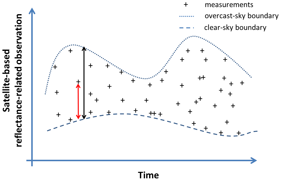
Figure 1The calculation of a cloud index for a given location. The cloud index is the ratio between the distances “measurement to clear sky” (red arrow) and “overcast sky to clear sky” (black arrow).
The cloud index concept is based on the idea that the presence of a cloud brightens locally pixels of satellite shortwave imagery. In general, the value that quantifies reflectances of a given location observed from the top of the atmosphere (TOA) is comprised between low and high boundary values. The low boundary value Xmin is taken as the clear-sky case and the high one Xmax as the cloudiest case. The attenuation of downwelling surface solar irradiance by clouds is roughly given as a linear function of the difference between the measured value Xsat and the clear-sky boundary relative to the difference between cloudy and clear-sky cases, as illustrated in Fig. 1. We name these variables X as they can be of a slightly different nature from one work to another (reflectance, albedo, radiance, digital count, etc.). The cloud index n is then given as
Differences between cloud index methods mainly rely on
-
modifications of the relationship between the cloud index and the effective cloud transmissivity (Zarzalejo et al., 2009; Perez et al., 2002; Gupta et al., 2001; Rigollier and Wald, 1998),
-
the choice of the variable used to calculate the cloud index, for example, TOA albedo (Darnell et al., 1988), reflectance (Wang et al., 2014; Gupta et al., 2001; Möser and Raschke, 1984), Lambert equivalent reflectivity (LER) (Herman et al., 2018; Dave, 1978), or raw satellite numerical counts (Müller et al., 2015; Perez et al., 2002; Cano et al., 1986), and
-
the way of retrieving Xmax and Xmin for the chosen variable.
Very different approaches are used to estimate the upper boundary, but for the lower boundary, “archive-based” methods are used in most of the literature we reviewed: Xmin is a minimum based on a time series of past satellite imagery. This approach has some drawbacks. Firstly, it is hardly applicable to non-geostationary satellites due to variable viewing geometries and a low revisit time. As an example, Wang et al. (2014) use a climatology of surface albedo to derive DSSI from the Ozone Monitoring Instrument (OMI), embedded on the Sun-synchronous satellite Aura. Secondly, systematic underestimations of the lower boundary Xmin are commonly detected, for example, due to dark shadowing caused by adjacent clouds on the surface and aerosol treatment (Mueller et al., 2015). On the other hand, contamination of Xmin by clouds in the cloudiest regions can lead to systematic overestimation of Xmin. Finally, ensuring the observation of clear-sky instants by a sufficiently large time window and capturing the temporal variability of Xmin by a sufficiently small time window is a difficult trade-off that can lead to biases if not well respected.
In this paper, we propose a cloud index method based on radiative transfer modeling as an alternative to the archive-based approach. This exploratory direction aims at reproducing the satellite measurements of reflectances in both clear-sky and overcast conditions based on description of surface, clear atmosphere, and cloud properties. Radiative transfer simulations are able to reproduce how TOA reflectances depend on viewing and solar geometries, also with their spectral distribution. In addition, it is possible to provide to the radiative transfer model input data that describe variations in space and time of clear atmosphere composition and of surface properties. Thus, our approach is useful for identifying and quantifying sources of errors in cloud index methods.
With a spectral and angular description, our method is also able to extend the application field of the cloud index approach to a wider variety of orbits and optical shortwave sensors. In order to limit the effects of molecular scattering, ozone absorption and polarization present in the ultraviolet, and the absorption of radiation by clouds in the near infrared, the method focuses on satellite imagery in the spectral range 400–1000 nm. This range is wide enough to consider imagers on many meteorological satellites launched since the beginnings of spaceborne Earth observation.
The method foreseen to compute the cloud index of Heliosat-V and eventually the DSSI is described in Sect. 2, along with the protocol of validation. Validation results are presented and discussed in Sect. 3 for simulated reflectances at the top of the atmosphere and for downwelling surface solar irradiance estimates. Section 4 is dedicated to the conclusion and perspectives.
Previous methods based on archives can avoid dependency on absolute calibration of the original imagery (Müller et al., 2015; Perez et al., 2002) and consider implicitly the anisotropy of Xmin. The pixel-to-pixel estimation of Xmin is a surrogate for modeling the influence of viewing geometry on measured reflectances, while the slot-by-slot temporal characterization of Xmin captures the influence of varying solar-viewing geometry for the diurnal cycle of each pixel's reflectivity. The development of an alternative to archive-based approaches means dealing with new issues: a challenge is to reproduce explicitly and accurately the TOA reflectances. For this, input data and models used need to satisfy the requirements for accurate DSSI estimations, as will be discussed hereafter.
2.1 The cloud index n
As stated in the introduction, Heliosat-V (HSV) is a method approximating the attenuation of DSSI radiation by clouds with a cloud index, n. Here, the cloud index components are reflectances considered at the TOA and corresponding to the satellite radiometer viewing geometry and spectral sensitivity. Reflectances are defined by the relation
with L the upwelling radiance at TOA for a given spectral channel, E0 the downwelling spectral solar irradiance at the top of the atmosphere on a perpendicular plane weighted by the spectral response function of the channel, and θs the solar zenith angle for a given location (i.e., latitude and longitude) and a given time. E0 varies mainly with the Sun–Earth distance, computed here with the Solar Geometry 2 algorithm (Blanc and Wald, 2012). The cloud index is then defined as
where ρsat is the reflectance measured by the radiometer for the given spectral channel, while ρclear and ρovc are estimates of the reflectance that would be measured by the same sensor for, respectively, a clear-sky scene and an overcast scene, i.e., with an optically thick cloud covering the whole pixel considered. The notion of “optically thick cloud” will be described in detail in Sect. 2.3.
Because of its definition, the cloud index may also be calculated with radiances. We consider here reflectances in order to visualize the anisotropic nature of different scenes. It also has the advantage of being a normalized quantity, so we can compare results for different radiometric channels and different solar zenith angles.
The relationship between n and DSSI varies slightly from one method to another, in particular for the highest and lowest values of n. The core of the relationship for intermediate values of n usually follows
where G is the all-sky DSSI and Gc is the DSSI in clear-sky conditions and is provided by an external model. The external model used in this paper will be presented and discussed in Sect. 2.4. The clear-sky index Kc is largely used to simplify the reading and is defined as
so we can rewrite Eq. (4) as
In this paper, we keep the original and simple relation introduced by Darnell et al. (1988). Its improvement is beyond the scope of this work but has been explored by various studies, e.g., by Rigollier and Wald (1998) (reported in Rigollier et al., 2004), Gupta et al. (2001), Perez et al. (2002), and Zarzalejo et al. (2009), notably to better characterize cloudy situations with n≈1. In the following subsections, we describe the method used to compute ρclear, ρovc, and Gc.
2.2 The clear-sky reflectances ρclear
We use a radiative transfer model to estimate what a spaceborne optical imaging system would measure in clear-sky conditions for a given radiometric channel. Using simulations in cloud indices has previously been done, notably to retrieve effective cloud fractions from the OMI (Lorente et al., 2018; Veefkind et al., 2016; Stammes et al., 2008). We apply the same approach to satellite radiometers.
Radiative transfer simulations are able to estimate reflected radiation at the top of the atmosphere (TOA) considering the non-Lambertian nature of the atmosphere and of Earth’s surfaces. For the implementation of the method applied here, we use the model uvspec within the software package libRadtran (version 2.0.2) (Emde et al., 2016) and the one-dimensional solver DISORT (Buras et al., 2011). We chose to use 32 streams for DISORT as a good compromise between time computation and a good angular representativeness of simulated radiances. For the spectral description, radiative transfer simulations are made following the so-called REPTRAN spectral approximation (Gasteiger et al., 2014). This parameterization enables the production of fast computations of radiative transfer adapted to the spectral sensitivity of satellite radiometric channels.
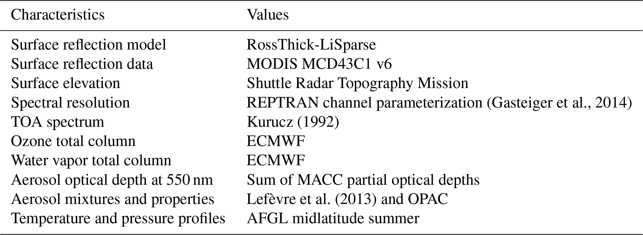
The spectral description of downwelling solar irradiance at the top of the atmosphere is provided by data from Kurucz (1992) for simulating ρclear. The composition of the atmosphere is provided by time series of total atmospheric columns of ozone and water vapor and partial aerosol optical depths (AODs) from the Monitoring Atmospheric Composition and Climate (MACC) reanalysis (Inness et al., 2013) distributed by the ECMWF. Data from MACC are extracted from the McClear service (http://www.soda-pro.com/web-services/radiation/cams-mcclear, last access: 16 January 2020). MACC values are originally given on a 3 h time step and with a spatial resolution of about 80 km (Inness et al., 2013; Lefèvre et al., 2013). The McClear service applies to MACC data a bilinear spatial interpolation onto the considered location and a linear interpolation in time to a 1 min time step (Lefèvre et al., 2013). The atmospheric abundance profiles of O2, CO2, and NO2 are kept to the fixed values of the Air Force Geophysics Laboratory (AFGL) midlatitude summer profile (Anderson et al., 1986) along with the temperature, pressure, and air density profiles.
Partial AODs from MACC are provided at the wavelength 550 nm for five types of aerosols (black carbon, dust, sea salt, organic matter, sulfate). Even though two supplementary classes “ammonium” and “nitrate” are now included in the Copernicus Atmospheric Monitoring Service (CAMS) reanalysis, these do not impact the method proposed here and were, thus, not considered.
An algorithm developed by Lefèvre et al. (2013) translates MACC partial aerosol optical depth information into aerosol mixtures designed for the Optical Properties of Aerosols and Clouds (OPAC) software package (Hess et al., 1998). These mixtures are associated with aerosol properties: scattering and absorbing coefficients, single scattering albedo, asymmetry parameter, and the Angström coefficient. The total AOD at 550 nm is then calculated as the sum of partial AOD at 550 nm provided by CAMS. As libRadtran needs a total AOD input for the simulated wavelength, the OPAC Angström coefficient of the given mixture is used to estimate the AOD at the required wavelength.
An important component to simulate ρclear is the reflection properties of surfaces. The impact of the anisotropy of surface reflectance has notably been shown for estimates of a cloud index derived from measurements of the ultraviolet/visible Global Ozone Monitoring Experiment 2 (GOME-2) and OMI by Lorente et al. (2018). This study also highlights the improvement of simulated shortwave clear-sky reflectances at the TOA when using a model of the bidirectional reflectance distribution function (BRDF) parameterized with data derived from the Moderate Resolution Imaging Spectroradiometer (MODIS) spaceborne instruments.
Here, we describe reflective properties of land surfaces with the RossThick-LiSparse (Ross–Li) model of the BRDF (Roujean et al., 1992; Lucht et al., 2000). It is then possible to consider the variations of the surface reflectance depending on the viewing and solar zenith angles and on the azimuthal difference of both geometries Δϕ. The Ross–Li model decomposes the BRDF of a surface into a sum of three components: an isotropic contribution, independent of viewing and solar geometries, a volumic contribution, following a mathematical model of an idealized canopy, and a geometric contribution, considering the shadows induced by the roughness of the surface.
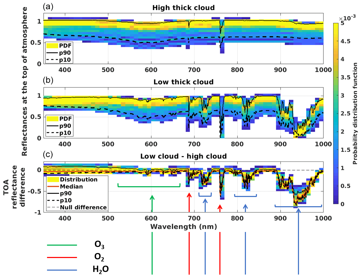
Figure 2(a, b) Distributions of simulated TOA reflectance spectra in overcast conditions ρovc for the different viewing geometries in the look-up table and for a solar zenith angle of 30∘, with a thick liquid cloud (COT =150). (a) CTH =15 km; cloud base height (CBH) =2 km. (b) CTH =0.5 km; CBH =0.2 km. (c) Error on ρovc caused by a misattribution of cloud height to the “low thick cloud” category. Green, red, and blue arrows indicate spectral regions with main absorption features from O3, O2, and H2O, respectively.
Algorithms have been developed to estimate the parameters fiso, fvol, and fgeo that weight, respectively, each of the contributors to the surface reflectance for all lands. This has notably been done with the imagery produced by MODIS embedded on the Terra and Aqua satellites (Wanner et al., 1997; Lyapustin et al., 2018).
We test here simulations with data from the Algorithm for Modeling MODIS Bidirectional Reflectance Anisotropies of the Land Surface (AMBRALS) (Wanner et al., 1997) with its derived product MCD43C1 v6 (Schaaf et al., 2002). This product provides fiso, fvol, and fgeo parameters with a 0.05∘ resolution (about 6 km at the Equator), a daily sampling rate, a 16 d average, and seven spectral channels, including four channels in the 400–1000 nm spectral interval considered for the Heliosat-V method (Fig. 3). Owing to libRadtran documentation (Mayer et al., 2017), the values of each parameter are assigned to the central wavelength of its channel, and a linear spectral interpolation is applied for the radiative transfer calculations. For wavelengths shorter than the 0.47 µm MODIS channel, values are considered spectrally constant. For wavelengths longer than 0.85 µm, the interpolation is made between parameters at MODIS channels 0.86 and 1.24 µm. A summary of inputs used to produce simulations of clear-sky reflectances is provided in Table 2.
2.3 The overcast-sky reflectances ρovc
Cloud index methods in the literature use various ways to estimate the TOA reflectances in overcast conditions ρovc (Perez et al., 2002; Lefèvre et al., 2007; Mueller and Träger-Chatterjee, 2014). One way to approximate it without the use of archives of satellite imagery has been proposed within the Heliosat-2 framework (Lefèvre et al., 2007) with an empirical relation based on the work of Taylor and Stowe (1984). It considers a dependency of ρovc with the single solar zenith angle θs.
However, spectral radiative transfer simulations of ρovc show that there is also a significant dependency between the TOA cloudy reflectances and other variables. In Fig. 2, we represent two-dimensional histograms of TOA reflectances calculated from such simulations, with a solar zenith angle set to 30∘ as an example. For most wavelengths, a significant spread of the distribution is observed (Fig. 2a and b), corresponding only to different viewing geometries defined by a linear mesh grid in the cosine of the viewing zenith angle (θv) and difference Δϕ of the solar and viewing azimuth angles (Table 1).
In this paper, we assume a cloud optical thickness (COT) of 150 to define optically thick clouds and overcast conditions. This assumption relies on COT statistics from Trishchenko et al. (2001). The simulations for a low thick cloud (cloud top height (CTH) at 500 m) and a high thick cloud (CTH at 15 km) show in general good agreement (Fig. 2c), except in absorbing bands of O2 (mainly at 690 nm, O2-B band, and 762 nm, O2-A band) and H2O (mainly at 725, 820, and 950 nm) and for short wavelengths where scattering becomes increasingly significant (e.g., Jin et al., 2011). For these wavelengths, the TOA reflectances with low clouds can be much lower than for high clouds for a given cloud optical thickness. However, outside these specific spectral regions, the height of clouds will not affect significantly the results of the method.
An alternative way is therefore to produce look-up tables (LUTs) from radiative transfer simulations, an approach notably applied in the framework of the HelioMont cloud index method (Stöckli, 2014). It is then possible to take into account the viewing geometry and also the spectral variability of ρovc. Assumptions have to be made about the properties of the optically thick clouds as the Heliosat-V method is designed to work by using only one spectral channel in the range 400–1000 nm: cloud top height, phase of cloud, cloud optical thickness, cloud droplet radius, or ice crystal shape and size.
Here we construct a liquid cloud LUT of ρovc, setting different cloud and atmosphere properties, geometries, and spectral grids, as described in Table 1. The optical properties of the clouds come from the precalculated Mie tables provided by the libRadtran software package.
As no information is provided on the actual cloud vertical structure, ρovc are calculated as
where ρovc,high and ρovc,low are reflectances, respectively, derived from the high and low liquid cloud LUTs, interpolated on the viewing and solar geometries of the satellite time series and adapted to the spectral response function of radiometric channels.
An ice cloud LUT is also produced to study the sensitivity of surface irradiance estimates to the assumed cloud phase. The ice cloud characteristics follow the parameterization by Yang et al. (2013). We use the “aggregate of eight columns” ice crystal habit and the “severe” degree of roughness, which are notably used for the description of ice clouds in the look-up table of the MODIS collection 6 cloud product (Amarasinghe et al., 2017).
Gueymard (2018)Shettle (1990)Table 1Characteristics of the look-up table of cloudy TOA reflectances.
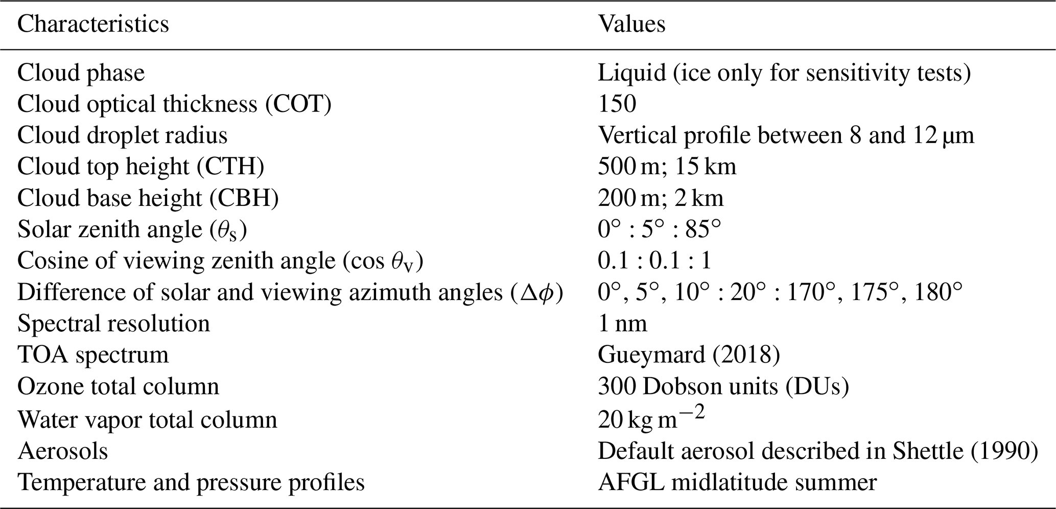
Table 2Characteristics of the simulated reflectances at the top of the atmosphere in clear-sky conditions.
2.4 The clear-sky model of surface irradiance Gc
The clear-sky surface irradiance is given by version 3 of the McClear model (Gschwind et al., 2019). The McClear model is a fast and accurate model that provides clear-sky estimation of DSSI with an absolute bias below 21 W m−2 and a standard deviation error below 25 W m−2 for six stations part of the reference Baseline Surface Radiation Network (BSRN) (Ohmura et al., 1998; Driemel et al., 2018), namely, Brasilia, Carpentras, Palaiseau, Payerne, Sede Boker, and Tamanrasset. The McClear model was fed with the partial optical depths at 550 nm for black carbon, dust, sea salt, organic matter, and sulfate from MACC reanalysis. It is also fed by water vapor atmospheric total columns and the ozone total columns provided by ECMWF. Data were downloaded from the McClear web service (http://www.soda-pro.com/web-services/radiation/cams-mcclear, last access: 16 January 2020).
2.5 Setup and datasets for validation
The method has been tested on images from the Spinning Enhanced Visible and Infra-Red Imager (SEVIRI) aboard the Meteosat-9 meteorological geostationary satellite belonging to the family of Meteosat Second Generation (MSG). We consider measurements in the solar channels 0.6 and 0.8 µm for the year 2011 and for 11 locations in the field of view of the satellite, corresponding to locations of pyranometric in situ sensors from the BSRN. We use the calibration gains provided by EUMETSAT that operates MSG. For sensors with a linear count response like MSG/SEVIRI (Doelling et al., 2018), the radiance Lsat is related to digital count C via , where C0 is the so-called space count.
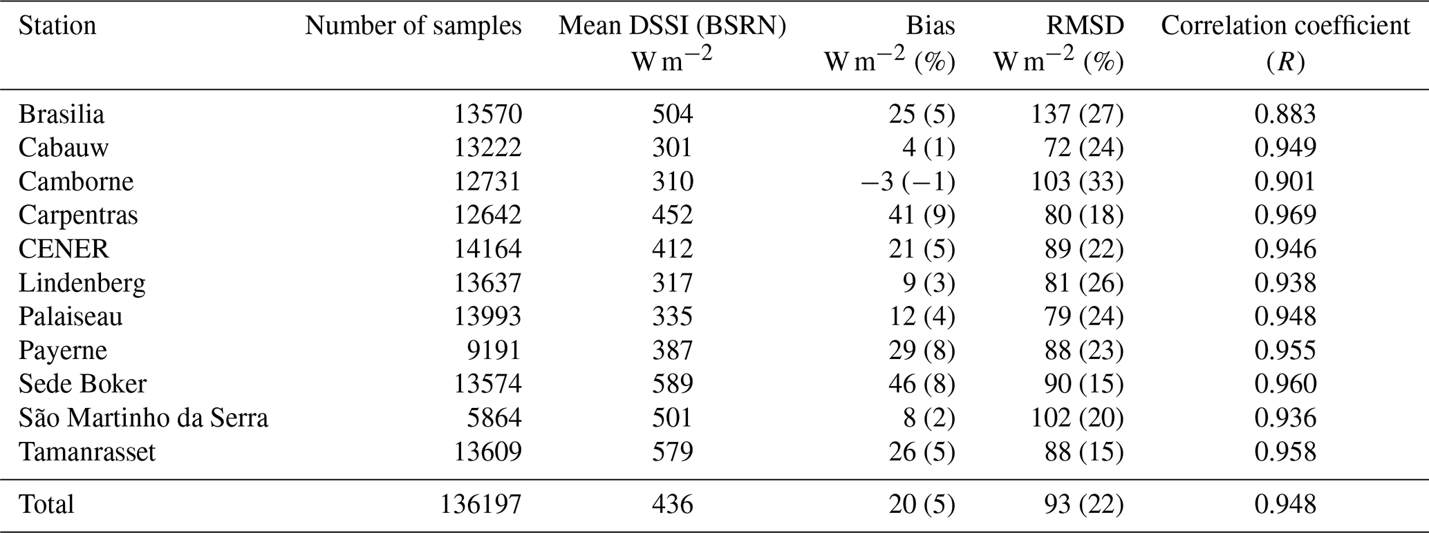
To study the validity of the method, we compare DSSI estimates from MSG satellite measurements with pyranometric DSSI data retrieved from BSRN measurement stations. Considered stations are listed in Table 3 and displayed in the MSG field of view in Fig. 4. Only the highest-quality BSRN measurements of surface irradiance are used, having passed a quality check (Lefèvre et al., 2013). Figure 5 shows the time series when data are considered valid, for each station.
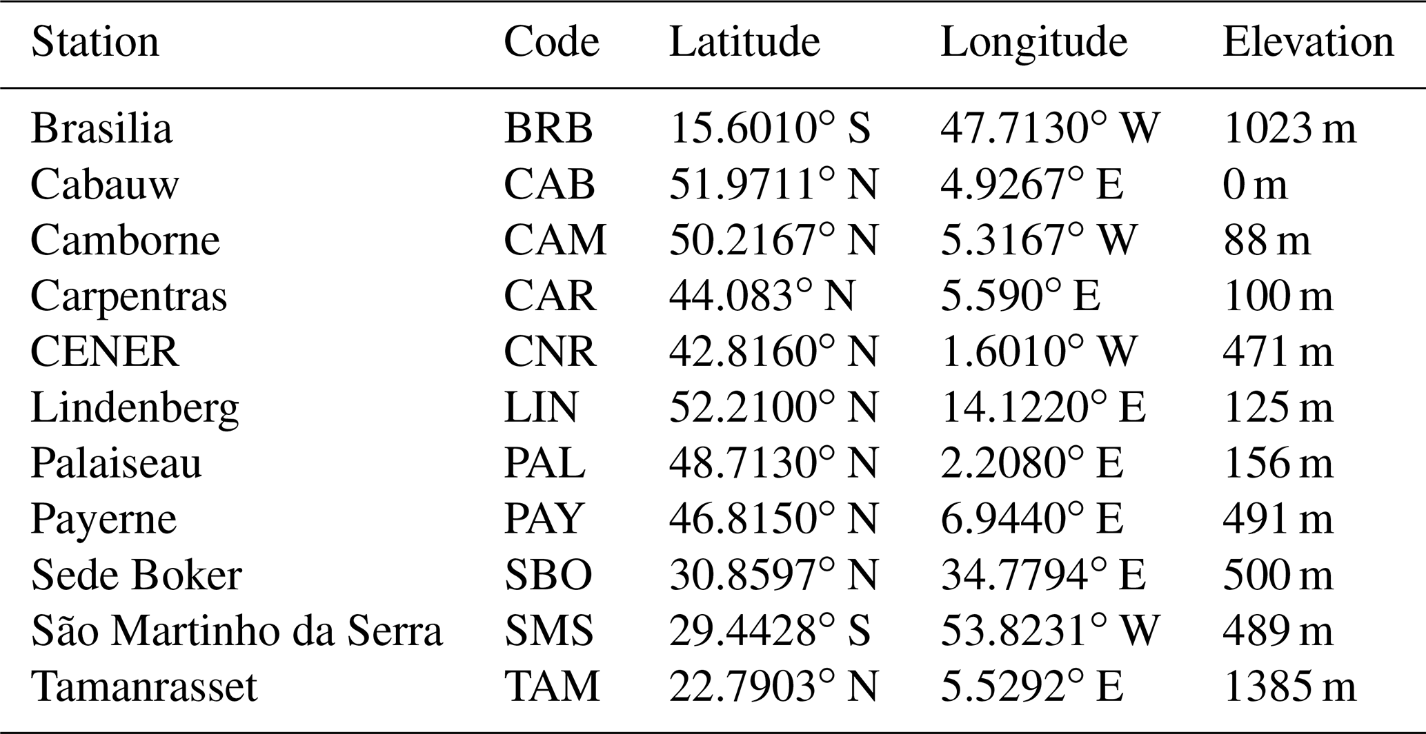
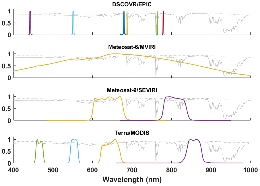
Figure 3Colored lines: spectral response functions of different sensors in the spectral range considered by Heliosat-V. Gray lines: TOA reflectance spectra of typical scenes with a high- (dashed line) and low-altitude (solid line) thick cloud.
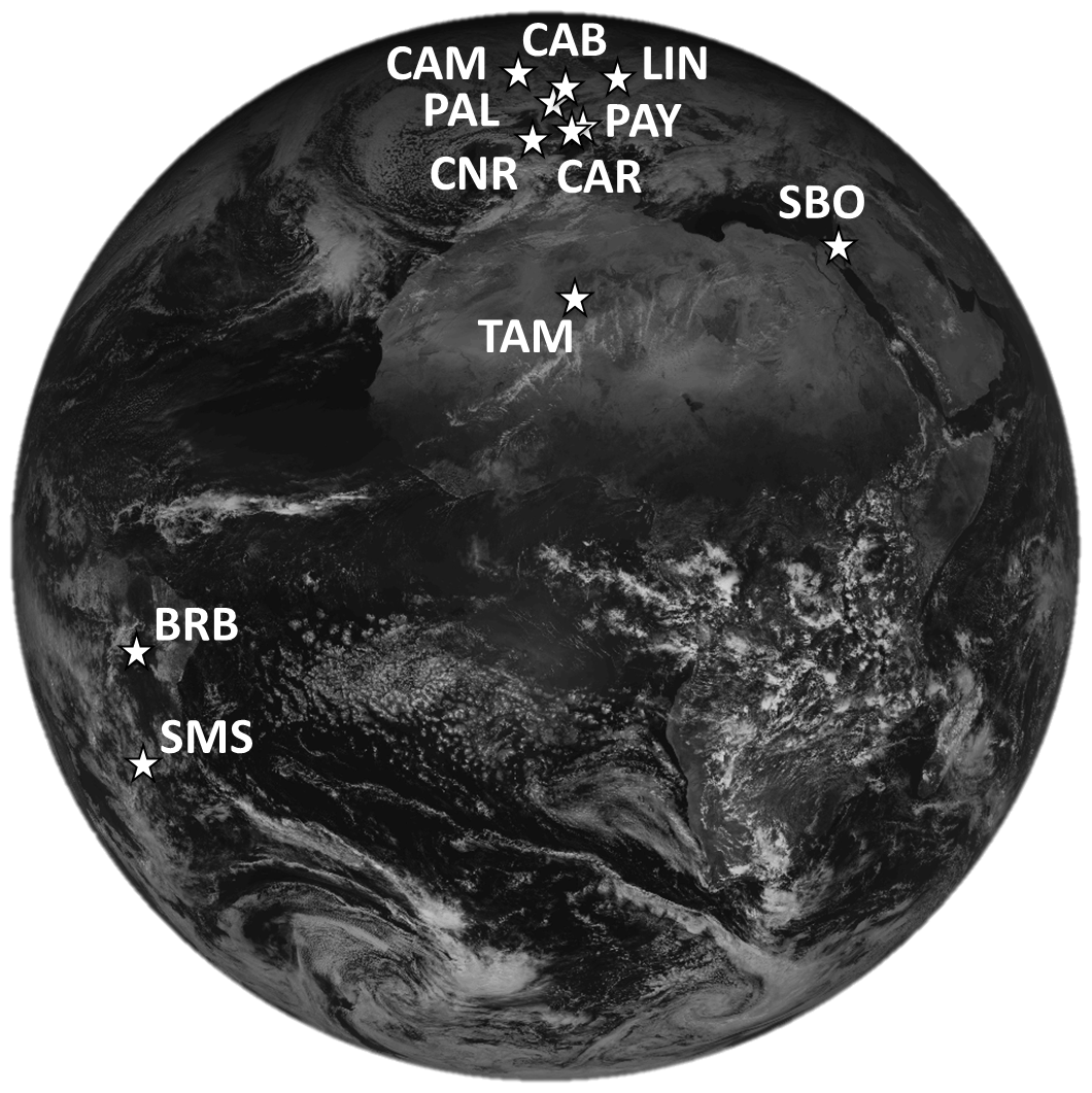
Figure 4BSRN ground stations used for validation in this study, in the field of view of Meteosat Second Generation (0.6 µm channel).
We also compare the results of our method to operational satellite-based products of surface irradiance. For this, we use data from the HelioClim3 version 5 (HC3v5) and CAMS Radiation (CAMS-RAD) DSSI databases. Both are derived from the imagery of the SEVIRI sensor and are produced by a Heliosat method: a modified version of Heliosat-2 for HC3v5 (Qu et al., 2014) and Heliosat-4 for CAMS-RAD. Both products and their descriptions are provided by the SoDa service (http://www.soda-pro.com/, last access: 9 September 2019).
As this work is exploratory on a new method, we limit ourselves to conservative situations with solar zenith angles lower than 80∘, covering most cases. For higher angles, some effects not considered by the method can occur, including shadowing and high parallax effects.
3.1 Validity of cloud index components
The validity of cloud index components, ρsat, ρclear, and ρovc, defines the uncertainty of n. From Eq. (3), the uncertainty in the cloud index can be written as
This leads to
where . It appears that the “clear-sky error” (1−n) δρclear will be more significant in clear-sky conditions (i.e., n is close to 0), and the “overcast-sky error” nδρovc will be more important in overcast conditions (i.e., n is close to 1). Besides, the error in the cloud index will be inversely proportional to Δ, the difference between overcast and clear-sky TOA reflectances. Because of this relationship between the errors in cloud index and reflectances, the discussions in this section are focused on absolute values of reflectance errors.
3.1.1 Measured reflectances at the top of the atmosphere
A potentially important source of the measurement error δρsat comes from the calibration gain. The operational calibration gains that we use in this paper have a claimed uncertainty of around 4 % (EUMETSAT, 2019). On the other hand, Hewison et al. (2020) assert that the alternative method by Doelling et al. (2018), used for GSICS-corrected computation of calibration gain, limits its bias to below 1 %.
The use of optimal calibration is beyond the scope of our work. Still, we compared gain coefficients proposed by EUMETSAT gEUM to those provided by Doelling et al. (2018) gD2018 for the measurements produced by the Meteosat-9 0.6 and 0.8 µm channels in 2011. They show a mean relative disagreement, calculated as , of about −9 % for 0.6 µm and −8 % for 0.8 µm during this period (also illustrated in Fig. A1). We expect that these errors will affect with the same magnitude the agreement between numerical simulations and measurements of clear-sky TOA reflectances. This underlines that an accurate source of absolute calibration is important for the Heliosat-V method.
3.1.2 Simulated reflectances at the top of the atmosphere in clear-sky conditions ρclear
As an intermediate assessment, simulated clear-sky reflectances at the top of the atmosphere (TOA) ρclear are compared to satellite measurements. Cloudy instants are manually filtered out of the satellite time series. Results comprising all the manually filtered clear-sky instants in 2011 for all 11 sites are shown in Fig. 6 as two-dimensional reflectance histograms.
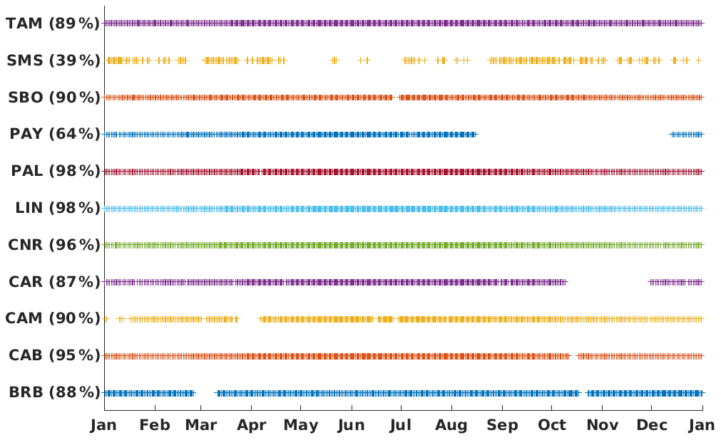
Figure 5Time series used for the 15 min mean statistics between satellite estimates and quality-checked BSRN measurements during the year 2011. In parentheses: percentage of data conserved.
For the 0.6 and 0.8 µm channels, correlation coefficients are both higher than 0.9, but the correlation is much better for 0.6 µm, with a value of 0.974. This means that the variability of ρclear is significantly better represented, with almost 95 % of the total variance, for 0.6 µm than for 0.8 µm, with 82 % of the total variance. The root-mean-square difference (RMSD) between the simulated reflectance and measured reflectance in the clear-sky conditions is 0.03 (15 %) for the 0.6 µm channel and 0.04 (12 %) for the 0.8 µm channel. The bias is 0.02 (10 %) and −0.02 (−7 %) for the 0.6 and 0.8 µm channels, respectively, contributing a big part to the RMSD. The standard deviation of the difference (SD) is 0.02 for the 0.6 µm channel and 0.04 for the 0.8 µm channel. Both higher bias and SD for the 0.8 µm will contribute to lowering the precision in the calculation of the cloud index based on this channel compared to 0.6 µm. When studying station by station, the highest absolute standard deviation of the difference between simulations and measurements is reached for Sede Boker with 0.03, while the lowest is reached for Tamanrasset with 0.008. For bias, the most significant mean values reach +0.035 for 0.6 µm (Payerne) and −0.07 for 0.8 µm (Camborne) (see also Fig. B1).
Using the gain coefficients developed by Doelling et al. (2018) for CERES-SYN1deg instead of EUMETSAT operational coefficients is sufficient to remove most of the mean bias observed between simulations and measurements of ρclear for the channel 0.6 µm. Besides, it increases the mean bias for the 0.8 µm channel.
It is worth noting that we use MCD43C1v6 BRDF data regardless of their quality flags. We observe though that keeping only the highest-quality data improves significantly statistics (Fig. B2). Also, the choice of a spectral linear interpolation between MODIS channels to simulate surface reflectances in SEVIRI channels is supposed to contribute significantly to biases observed in ρclear simulations, in particular for the 0.8 µm channel with vegetated surfaces due to the red edge spectral pattern (low reflectivity below around 700 nm, high reflectivity above around 750 nm). Another part of the bias, difficult to quantify, is linked to the accuracy of the calibration of satellite measurements.
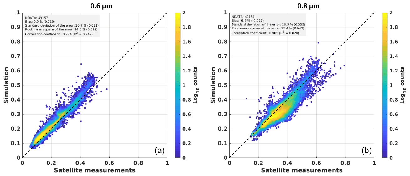
Figure 6Simulation of clear-sky reflectances at the TOA (ρclear) for MSG 0.6 µm (a) and 0.8 µm (b) spectral channels compared to actual satellite measurements. Represented data include simulations and measurements for all 11 locations, for the year 2011.
Figure 7 shows the diurnal variations of measured and simulated reflectances for the SMS and CAM stations. Both SMS and CAM are surrounded mainly by various types of vegetation and some urban area in the case of CAM (Fig. B3). We observe that simulations are able to reproduce partly the diurnal variability observed in clear-sky conditions (also refer to Fig. B4 for channels 0.6 and 0.8 µm under different surface conditions). In Fig. 8, we compare ρclear values to the surface reflectance ρsurface, computed with the RossThick-LiSparse model applied to BRDF parameters derived from the MODIS 646 nm channel and using the viewing and solar geometries considered. Firstly, we see that ρclear values are significantly higher than ρsurface, with a different diurnal pattern. This shows the importance of considering the atmosphere anisotropic reflectance to reproduce TOA reflectances. We can also see the contribution from the surface anisotropy in the ρclear simulations. This appears in particular close to the backscattering direction, where surface reflectance is enhanced: around noon in Camborne and the morning in São Martinho da Serra.
For CAM, some higher values of ρclear are observed in January. This can be attributed to high aerosol optical depth during this period, as illustrated in Fig. 9. It shows that ρclear is not only sensitive to time variations of surface properties, but also to atmospheric composition changes.
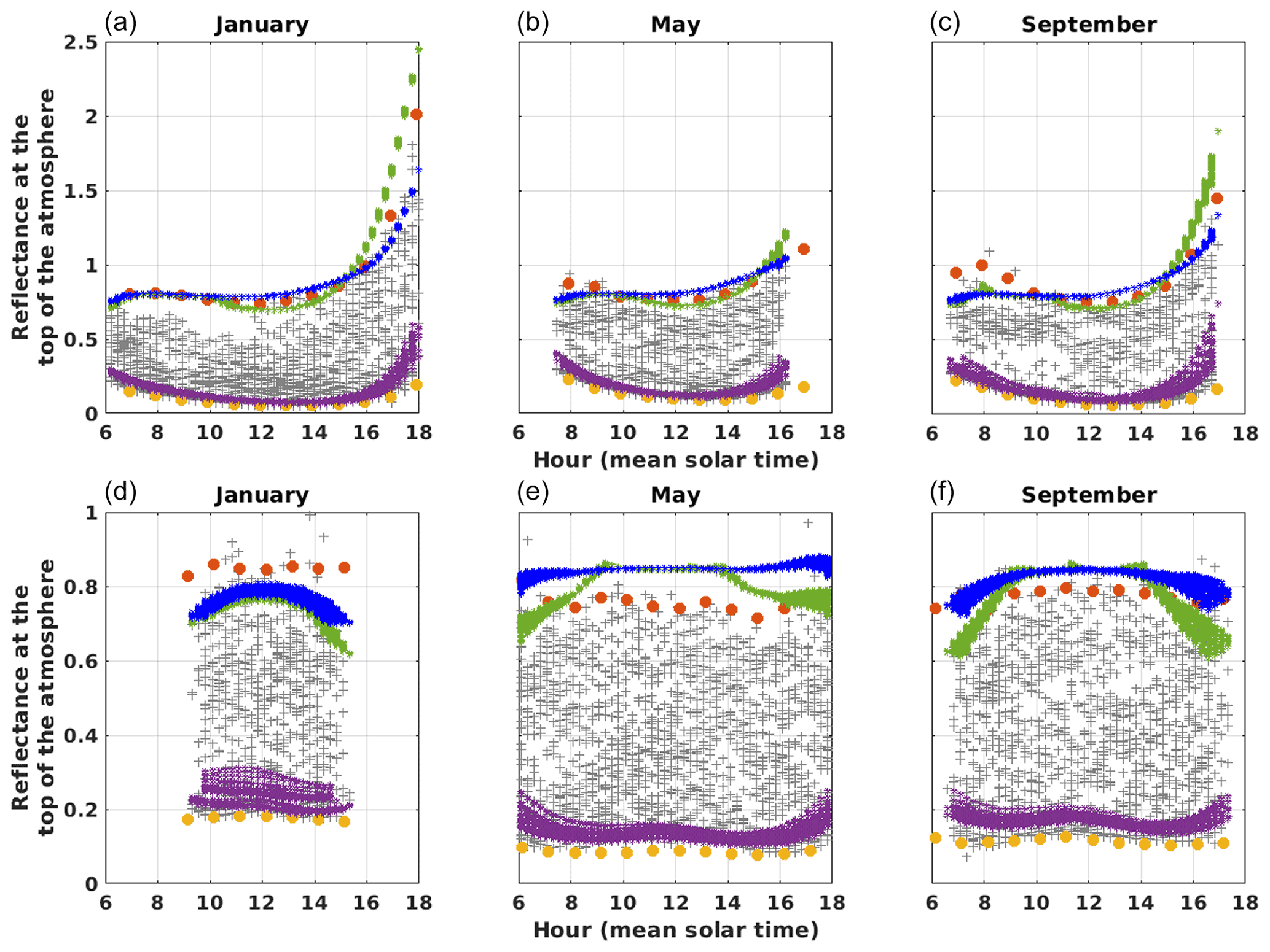
Figure 7Simulated and measured reflectances at the top of the atmosphere above the São Martinho da Serra (Brazil, a–c) and Camborne (United Kingdom, d–f) locations, for the MSG 0.6 µm channel and for the January, May, and September calendar months. Gray plus signs: MSG measurements (2011, Meteosat-9). Green asterisks: reflectances in overcast conditions ρovc, derived from the liquid cloud look-up table. Blue asterisks: same from the ice-cloud look-up table. Purple asterisks: reflectances in clear-sky conditions ρclear, derived from radiative transfer simulations. Yellow and orange dots are, respectively, hourly percentiles 1 and 99 of MSG satellite measurements from years 2011 to 2019.

Figure 8Comparison between simulations of clear-sky reflectances at the top of the atmosphere for the MSG 0.6 µm channel (ρclear, blue plus signs) and corresponding surface reflectances computed with the RossThick-LiSparse model applied to MODIS MCD43C1v6 BRDF parameters for the channel 646 nm (ρsurface, red plus signs) for 5 d in June 2011. (a) Camborne station (CAM); (b) São Martinho da Serra station (SMS).
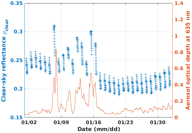
Figure 9Blue plus signs: simulated reflectances at the top of the atmosphere in clear-sky conditions ρclear in January 2011 at Camborne station (CAM) and for MSG 0.6 µm. Red line: aerosol optical depth at 635 nm used for simulations.
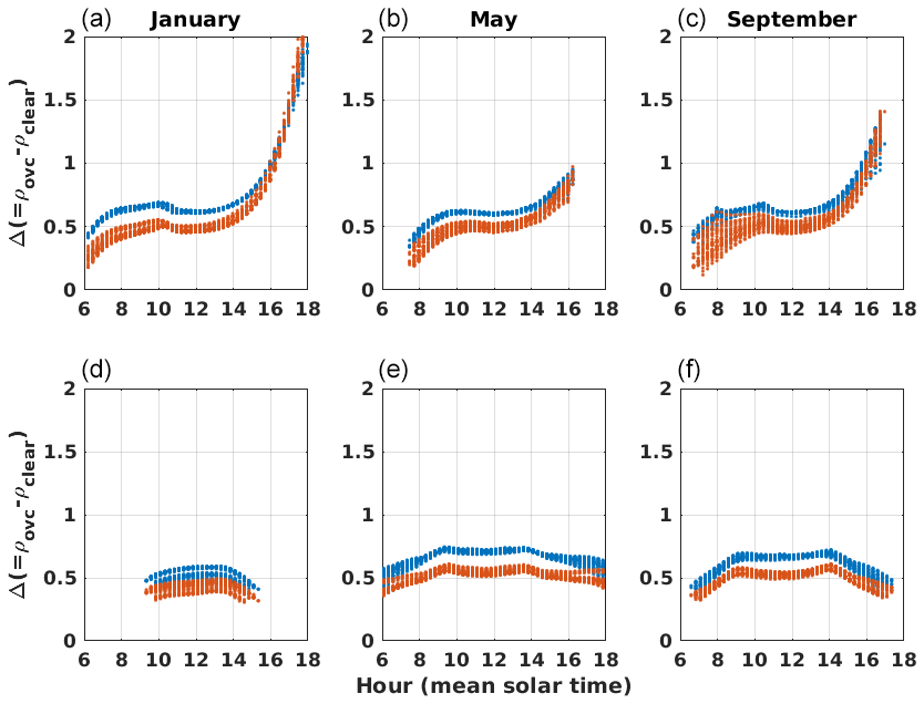
Figure 10Difference between simulated reflectances at the top of the atmosphere in overcast and clear-sky conditions for the São Martinho da Serra (Brazil, a–c) and Camborne (United Kingdom, d–f) locations and for the January, May, and September calendar months (a, d; b, e; c, f). In blue dots: MSG 0.6 µm channel; in red dots: MSG 0.8 µm channel.
3.1.3 Simulated reflectances at the top of the atmosphere in overcast conditions ρovc
The validity of ρovc is more difficult to test than that of ρclear by comparison to satellite measurements as the occurrence of optically thick clouds can be rare depending on the location, the season, and the hour of the day. We therefore use 9 years of Meteosat measurements between 2011 and 2019 to extract the 1 % most reflective scenes for each station, month, and hour of the day (orange dots in Fig. 7). In the first row of Fig. 7, we can see that some patterns are similar in simulated ρovc and the 99th percentile of measurements over the São Martinho da Serra pixel: in the forward-scattering conditions (evening on the western edge of the Meteosat disc), both agree on increased values of ρovc. On the other hand, some stations show regular values of measured reflectances beyond the ρovc simulated boundary, as in the example of Camborne (Fig. 7, second row). Figure 7 also illustrates how ρovc depends on the liquid or ice phase of the cloud, due to their different scattering phase functions. Our ability to reproduce reflectances at the top of the atmosphere in overcast conditions depends therefore on our knowledge of cloud properties, including their scattering phase function and top height. Other effects like the tridimensional structure of clouds probably explain part of the discrepancies between measurements and plane-parallel simulations in overcast conditions (Horvath and Davies, 2004).
3.1.4 Difference between simulated overcast and clear-sky reflectances
The difference Δ between overcast and clear-sky reflectances is bigger when the overcast reflectance is relatively low and clear-sky reflectance is relatively high. High values of Δ mean a good quality of cloud index estimation (cf. Eq. 9). We study the dependencies of Δ with the simulated reflectances to identify conditions that will cause high uncertainties in the computation of the cloud index. In general, we observe that the computed value of Δ is higher for the 0.6 µm channel than for 0.8 µm as a combination of surface, cloud, and clear atmosphere spectral signatures. This is illustrated in Fig. 10 for stations SMS and CAM. We observe however for the desert stations TAM and SBO that both channels present similar values of Δ (Fig. B5). Δ also depends on the viewing and solar geometries because of ρovc and ρclear different angular signatures. It leads, for example, for the SMS station and channel 0.8 µm to low values of Δ in January mornings and high values of Δ in the evening, which can be explained by the strong forward scattering of clouds occurring in these conditions.
3.2 Comparison of satellite-based estimates of DSSI to ground-based measurements
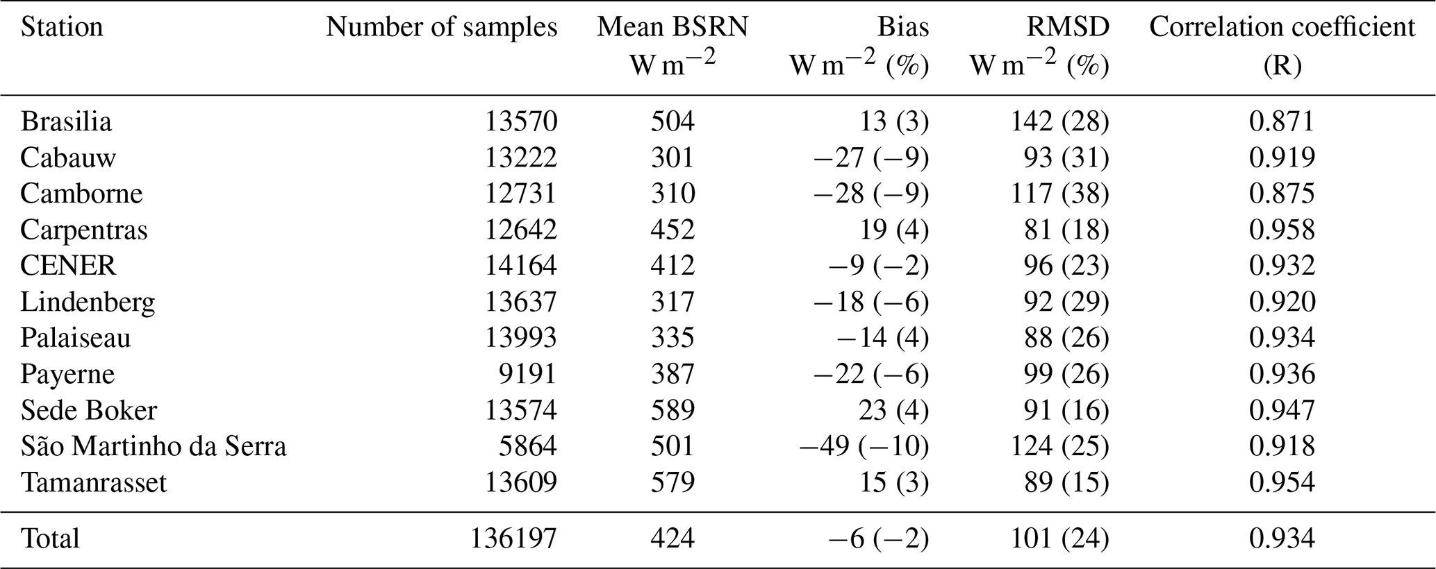
Validation results are shown in Table 4 for 15 min-averaged DSSI estimates. Satellite-based estimates are obtained with MSG 0.6 µm imagery. Results for MSG 0.8 µm imagery show generally lower quality in terms of correlation and SD, as shown in Fig. 11.
The simple relationship between the cloud index and the clear-sky index used here explains the significant number of negative values of DSSI estimates. The improvement of this relation will be the object of a future study.
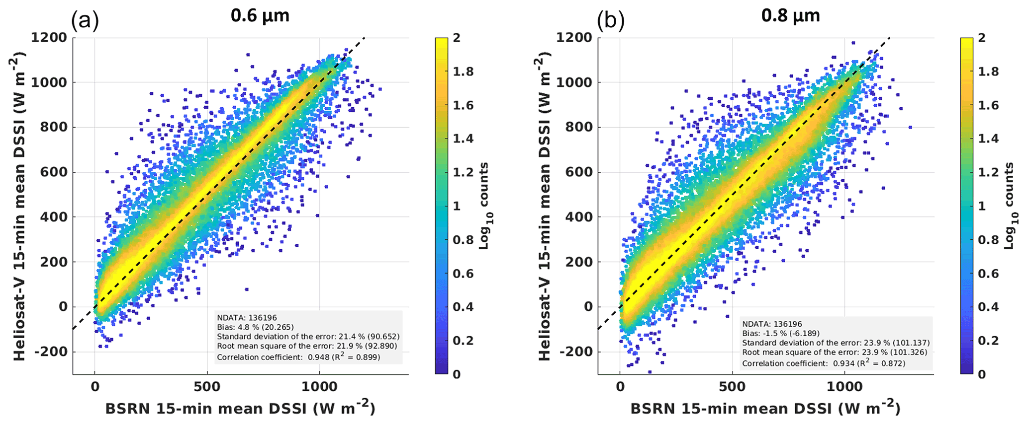
Figure 11Two-dimensional histograms of satellite-based DSSI estimates from the Heliosat-V method versus ground-based BSRN measurements for the MSG 0.6 µm channel (a) and 0.8 µm channel (b).
We tested the sensitivity of the DSSI estimates to the cloud phase by using in one case the reference look-up table, featuring a liquid cloud, and for the test case, an ice cloud as described in Sect. 2.3. Results show only minor differences, pointing out a limited influence of the cloud phase on DSSI estimates (Fig. B6).
Finally, the quality of the results also depends on the quality of the clear-sky surface irradiance model. Gschwind et al. (2019) report, for example, relative mean biases of the McClear model from −3.6 % (Barrow, Alaska, USA) to +3.2 % (Payerne, Switzerland) when compared to BSRN irradiance measurements. The improvement towards a least-biased estimation of the downwelling surface solar irradiance based on a cloud index will require better estimates of the attenuation of the solar radiation by the clear atmosphere.
Table 4Validation results for 15 min means of all-sky DSSI for the year 2011. Results based on the imagery of the Meteosat-9/SEVIRI 0.6 µm channel.
3.3 Comparison of satellite-based estimates of DSSI to the HelioClim3 and CAMS radiation products
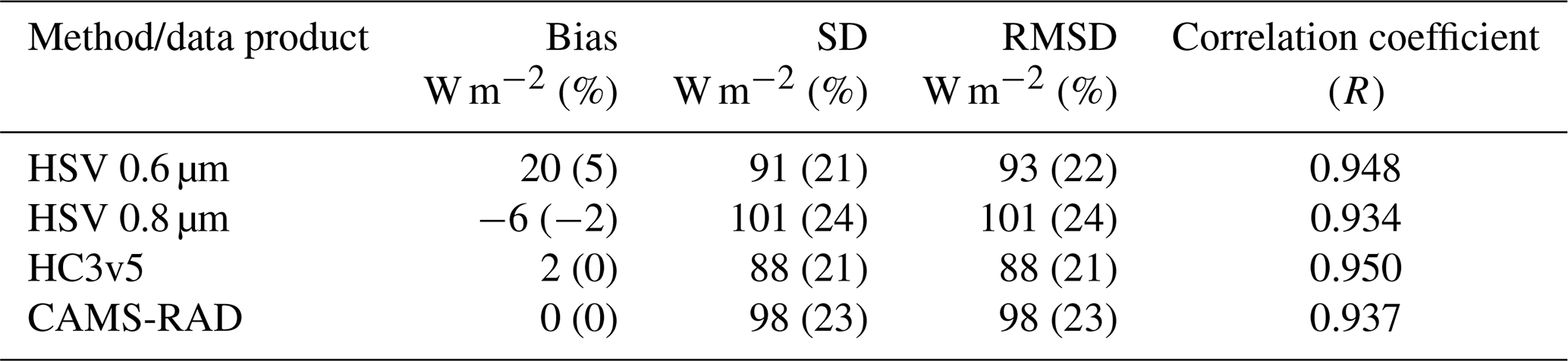
The results of the method are also compared to satellite-based DSSI products HelioClim3 version 5 (HC3v5) and CAMS Radiation Service (CAMS-RAD) in Table 5. Results for the new HSV method show statistics similar to HC3v5 and CAMS-RAD, for both estimates based on the 0.6 and 0.8 µm channels, in terms of correlation and of SD. One may note very low values of bias for operational products. This is expected because CAMS-RAD and HC3v5 estimates are calibrated with DSSI measurements from a similar set of BSRN stations.
Better results from the channel 0.6 µm could be attributed to a smaller influence of the cloud top height compared to the 0.8 µm channel which is affected by water vapor absorption (Fig. 3). Biases discussed for the computation of clear-sky and overcast TOA reflectances could also affect significantly DSSI estimates.
Table 5Comparison between validation results of HSV and those of HC3v5 and CAMS-RAD, each one versus BSRN measurements. Statistics on 15 min means of DSSI for the stack of 11 stations and the year 2011. N=135107; BSRN mean = 424 W m−2.
Heliosat-V is a cloud-index method for estimating downwelling surface solar irradiance from satellite imagery. In the framework of its development, we proposed an alternative way of retrieving the components of the cloud index, this index being used to quantify the attenuation of DSSI by clouds. The method takes advantage of radiative transfer modeling to provide versatility to the concept of the cloud index. Thus, it does not need archives of data to quantify the cloud effective transmissivity. It is applicable for optical sensors on geostationary and non-geostationary orbits; flexible for future improvements to describe surface, clear atmosphere, and clouds; and investigates physical solutions for limitations observed in previous cloud index methods.
It is built to deal with a single radiometric channel in the spectral range 400–1000 nm. The approach has the potential to deal with long time series of imagery from radiometers characterized by different spectral sensitivities and viewing geometries.
Validation results using SEVIRI imagery show that DSSI can be estimated by a cloud-index method that does not rely on archives of imagery, with a quality similar to operational satellite-based data products like the CAMS Radiation Service and HelioClim3 in terms of RMSD and correlation. This is an encouraging step toward the application of a Heliosat method to non-geostationary satellite sensors. However, we note that there are differentiated errors depending on the spectral channel considered. This could be attenuated notably by external knowledge of cloud top height and by improving the spectral interpolation of reflection properties of vegetated surfaces.
To clarify the potential of the method for long time series of imagery, we will need to explore how sensitive the results are to the quality of input data. The knowledge of atmospheric composition in absorbing and scattering species and on surface reflectivity properties is notably lower for past periods like the 1980s than for today. Also, the absolute calibration of satellite imagery can be more uncertain, without on-orbit calibrated instruments. Many inputs of the method have very different degrees of quality, depending on the period considered: the composition of the clear-sky atmosphere (aerosols and gases), surface properties, and external clear-sky irradiance model. Further work is still to be done on multidecadal time series to study how the quality of such ancillary data affect the estimates of DSSI.
Also, producing global maps of DSSI requires users to deal with non-geostationary satellite imagery. The first tests of the method have been done on the imagery of the Earth Polychromatic Imaging Camera (EPIC) embedded on the DSCOVR platform. They show encouraging results that will be extended and detailed in a future publication.
Global coverage of DSSI information obviously also requires users to deal with ocean surfaces and snow-covered regions, and this will need to be treated in the future.
A1 Setup of validation

Figure A1First two rows: calibration gains provided by EUMETSAT (black stars) and by CERES-SYN1deg (Doelling et al., 2018) (red stars) for the 0.6 µm channel (first row) and 0.8 µm (second row) of the SEVIRI sensor aboard Meteosat-9 between 2011 and 2019. Third row: ID of the operational satellite at longitude 0∘.
B1 Simulated TOA clear-sky reflectances ρclear
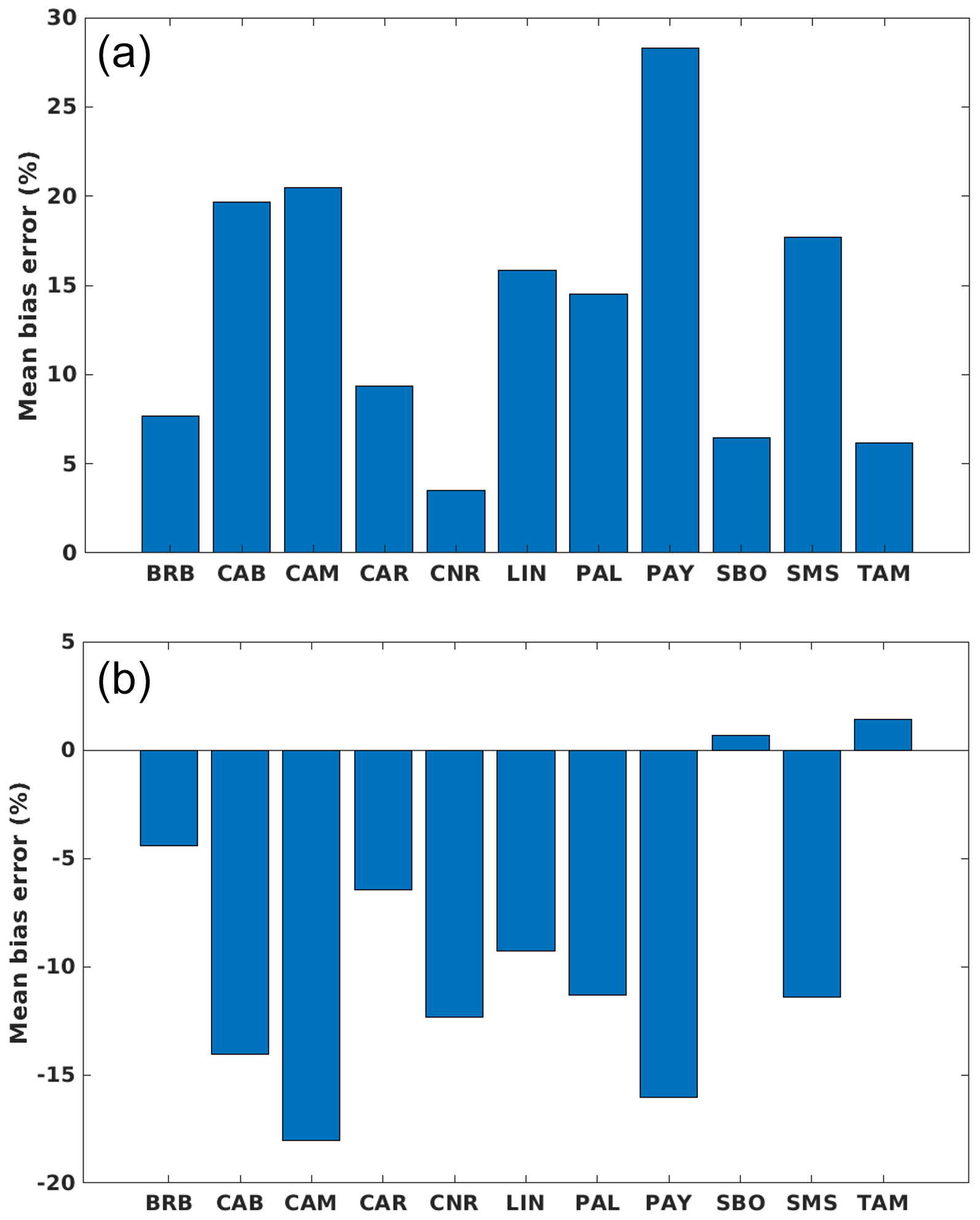
Figure B1Relative mean bias errors of simulated clear-sky reflectances at the top of the atmosphere ρclear (simulation measurementmeasurement) for channels 0.6 µm (a) and 0.8 µm (b) and for each BSRN site.
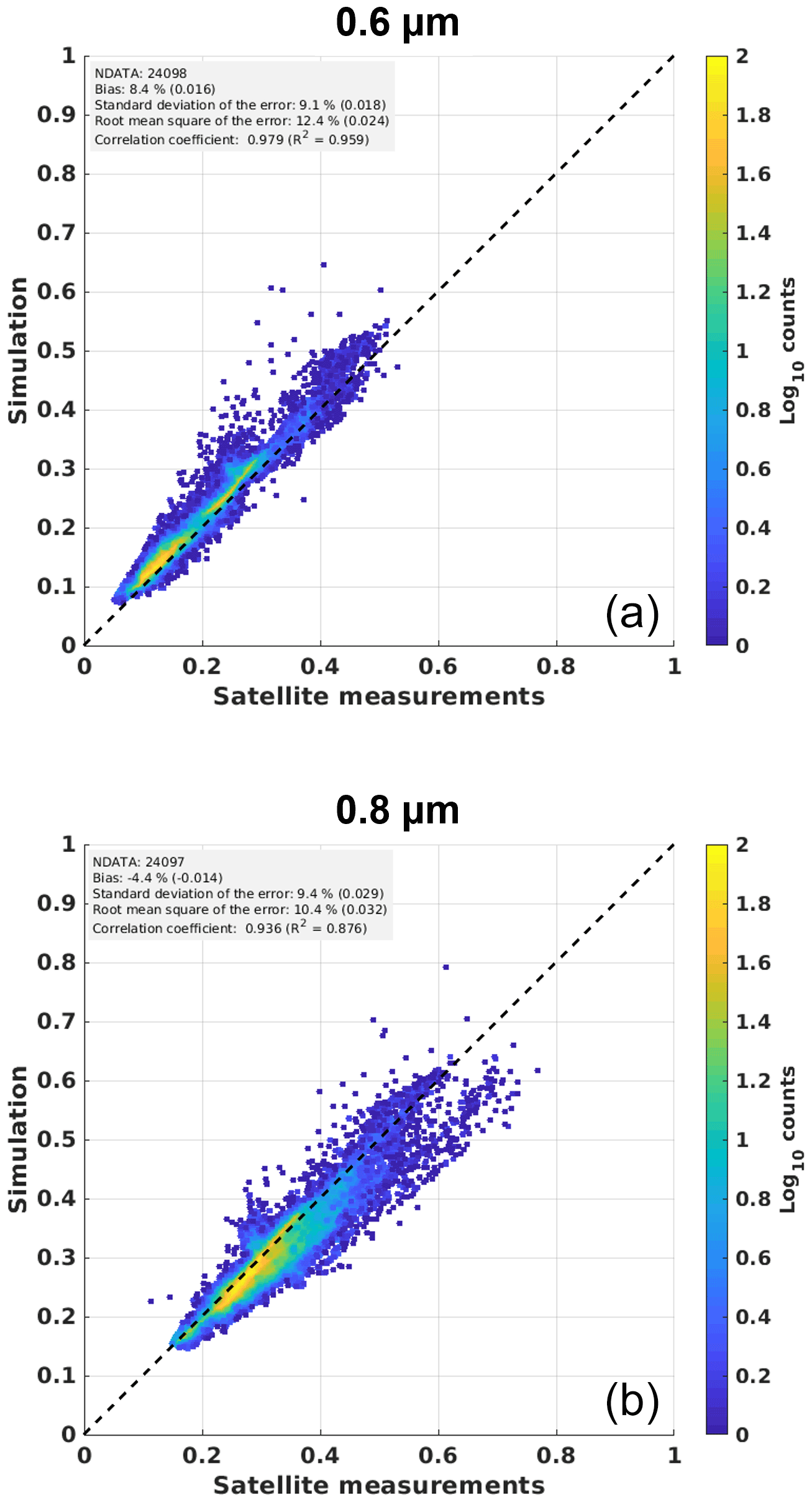
Figure B2Simulation of clear-sky reflectances at the top of the atmosphere (ρclear) for MSG 0.6 µm (a) and 0.8 µm (b) spectral channels compared to actual satellite measurements. The comparison is done for all 11 locations, for the year 2011. Only instants with BRDF data of the best quality are used (quality flag 0 of MCD43C1, “Best quality, 100 % with full inversion”).
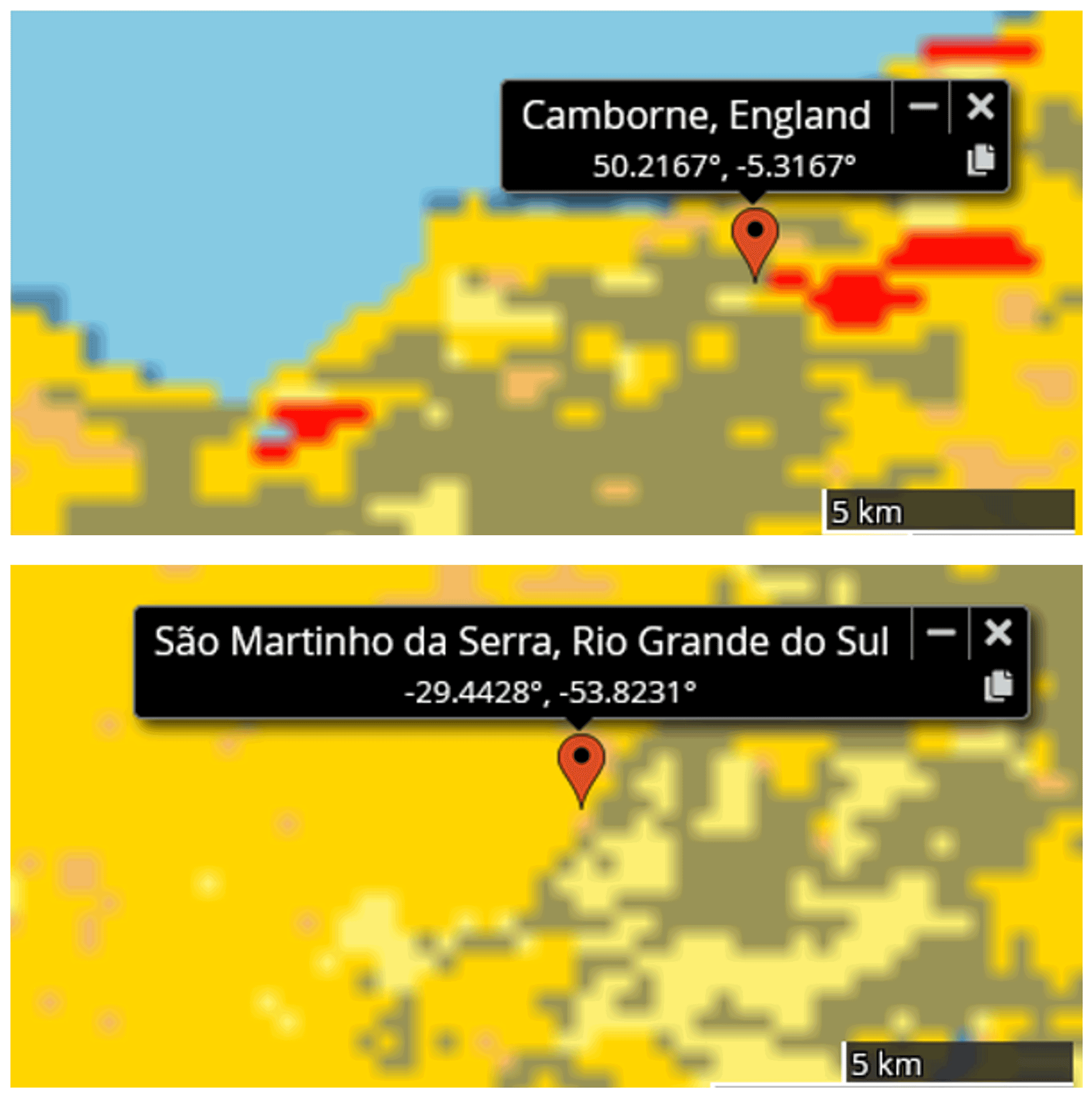
Figure B3Land cover types around measurement stations São Martinho da Serra (Brazil, upper panel) and Camborne (United Kingdom, lower panel) for 2011. In red: urban and built-up lands; in gray: croplands/natural vegetation mosaics; in light yellow: croplands; in dark yellow: savanna; in beige: grasslands; in blue: water bodies. Data from Terra + Aqua MODIS product MCD12Q1 version 6, following the International Geosphere-Biosphere Programme classification scheme (credit: NASA Worldview).
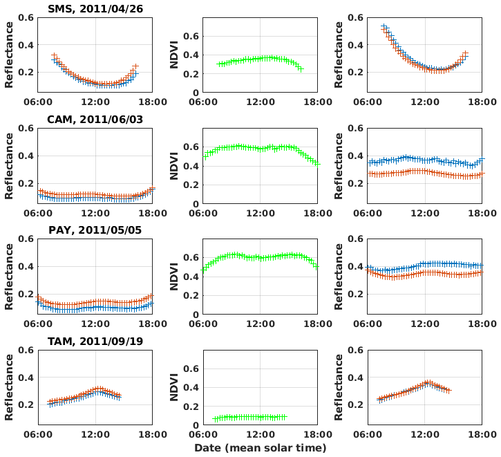
Figure B4Comparison between simulated (red plus signs) and measured reflectances (blue plus signs) at the top of the atmosphere for 1 d in clear-sky conditions, for the 0.6 µm (first column) and 0.8 µm channels (third column). NDVI computed from satellite measurements is shown in the second column. Rows from top to bottom: locations of the São Martinho Da Serra, Camborne, Payerne, and Tamanrasset BSRN stations.
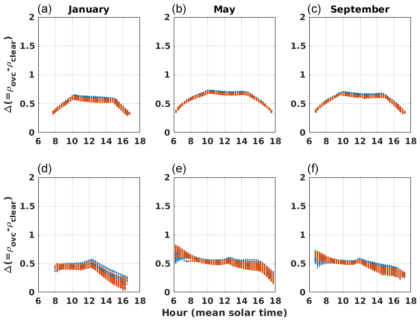
Figure B5Difference between simulated reflectances at the top of the atmosphere in overcast and clear-sky conditions for the Tamanrasset (Algeria, a–c) and Sede Boker (Israel, d–f) locations and for the January, May, and September calendar months (a, d; b, e; c, f). In blue dots: MSG 0.6 µm channel; in red dots: MSG 0.8 µm channel.
Table B1Validation results for 15 min means of the all-sky DSSI for the year 2011. Results based on the imagery of the Meteosat-9/SEVIRI 0.8 µm channel.
B2 Comparison of satellite-based estimates with ground-based measurements
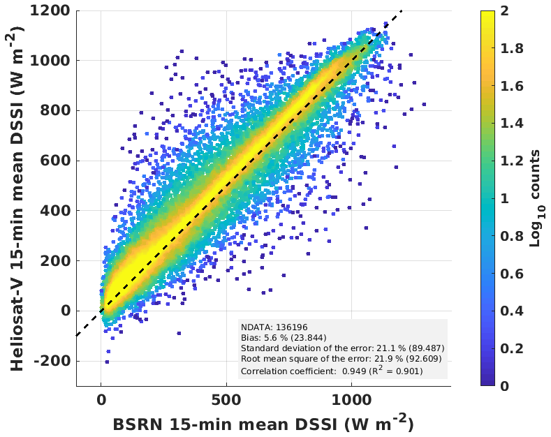
Figure B6Impact of the cloud phase on DSSI estimates. Two-dimensional histogram of satellite-based DSSI estimates from the Heliosat-V method versus ground-based BSRN measurements for the MSG 0.6 µm channel. The liquid cloud look-up table of overcast-sky TOA reflectances is replaced for the ice cloud LUT.
Excerpts of code are publicly available at https://doi.org/10.23646/tg31-1452 (Tournadre and Gschwind, 2022).
DSSI results derived from the implementation of Heliosat-V for validation on all 11 stations are publicly available at https://doi.org/10.23646/tg31-1452 (Tournadre and Gschwind, 2022), along with simulated and MSG measured reflectances, cloud and clear-sky indices, and clear-sky irradiance estimates from the McClear model. The manually filtered clear-sky instants are also provided for all 11 locations.
Conceptualization was done by BT, YMSD, and PB. Investigation, validation, and writing of the original draft were done by BT. Visualization was done by BT and PB. BT and BG did the software, with contributions from PB. Supervision was by PB and BG. Methodology was done by BT, PB, and YMSD. All the authors brought contributions to the writing process. XC and RAES brought contributions to the writing process, as did other co-authors.
The Transvalor company that partially funds this work distributes HelioClim3 and CAMS Radiation Service.
Publisher’s note: Copernicus Publications remains neutral with regard to jurisdictional claims in published maps and institutional affiliations.
We would like to thank the operators of the BSRN stations for producing and providing valuable validation measurements. We are grateful to the libRadtran team for their open radiative transfer model and interactions. The MODIS MCD43C1 version 6 data product was retrieved from the online NASA Earthdata Search, courtesy of the NASA EOSDIS Land Processes Distributed Active Archive Center (LP DAAC) and USGS/Earth Resources Observation and Science (EROS) Center, Sioux Falls, South Dakota, https://search.earthdata.nasa.gov/ (last access: 8 July 2019). We also thank EUMETSAT and the ECMWF for providing, respectively, Meteosat-9 and MACC reanalysis aerosol, water vapor, and ozone data. We used imagery from the NASA Worldview application (https://worldview.earthdata.nasa.gov, last access: 24 February 2022), part of the NASA Earth Observing System Data and Information System (EOSDIS). We thank Lionel Ménard for his help in the distribution of data linked to the paper (see the Data availability section). We thank the three anonymous reviewers for their helpful comments and suggestions. We finally thank Olivier Boucher, Alba Lorente, François-Marie Bréon, Jérome Vidot, Nicolas Ferlay, Philippe Dubuisson, Maximilien Patou, Alexander Marshak, Alexei Lyapustin, Jay Herman, Yuekui Yang, Tamas Varnai, Richard Perez, Paul Stackhouse, Seiji Kato, David Doelling, and Bastiaan Van Diedenhoven for useful discussions.
Benoît Tournadre was funded for his PhD work 50 % by Region Sud (grant no. 2017_05720) and 50 % by Transvalor SA (950 Avenue Roumanille, CS 40237 Biot, 06904 Sophia Antipolis Cedex France). The postdoctoral research fellowships of Benoît Tournadre and Xuemei Chen are funded by Transvalor SA.
This paper was edited by Piet Stammes and reviewed by three anonymous referees.
Amarasinghe, N., Platnick, S., and Meyer, K.: Overview of the MODIS Collection 6 Cloud Optical Property (MOD06) Retrieval Look-up Tables, NASA GSFC Cloud Retrieval Product Team, https://atmosphere-imager.gsfc.nasa.gov/sites/default/files/ModAtmo/C6_LUT_document_final.pdf (last access: 6 February 2020), 2017. a
Anderson, G., Clough, S., Kneizys, F., Chetwynd, J., and Shettle, E.: AFGL Atmospheric Constituent Profiles (0.120 km), Air Force Geophysics Laboratory, Hanscom Air Force Base, Bedford, Mass., Technical Report AFGL-TR-86-0110, 1986. a
Beyer, H. G., Costanzo, C., and Heinemann, D.: Modifications of the Heliosat procedure for irradiance estimates from satellite images, Sol. Energy, 56, 207–212, https://doi.org/10.1016/0038-092X(95)00092-6, 1996. a
Blanc, P. and Wald, L.: The SG2 algorithm for a fast and accurate computation of the position of the Sun for multi-decadal time period, Sol. Energy, 86, 3072–3083, https://doi.org/10.1016/j.solener.2012.07.018, 2012. a
Buras, R., Dowling, T., and Emde, C.: New secondary-scattering correction in DISORT with increased efficiency for forward scattering, J. Quant. Spectrosc. Ra., 112, 2028–2034, https://doi.org/10.1016/j.jqsrt.2011.03.019, 2011. a
Cano, D.: Etude de l'ennuagement par analyse de séquences d'images de satellite: application à l'évaluation du rayonnement solaire global au sol, PhD thesis, Ecole Nationale Supérieure des Mines de Paris, 1982. a
Cano, D., Monget, J., Albuisson, M., Guillard, H., Regas, N., and Wald, L.: A method for the determination of the global solar radiation from meteorological satellite data, Sol. Energy, 37, 31–39, https://doi.org/10.1016/0038-092X(86)90104-0, 1986. a, b
Cox, S. J., Stackhouse, P. W., Gupta, S. K., Mikovitz, J. C., and Zhang, T.: NASA/GEWEX shortwave surface radiation budget: Integrated data product with reprocessed radiance, cloud, and meteorology inputs, and new surface albedo treatment, in: AIP Conference Proceedings, Auckland, New Zealand, 16–22 April 2016, 1810, 090001, https://doi.org/10.1063/1.4975541, 2017. a
Darnell, W. L., Staylor, W. F., Gupta, S. K., and Denn, F. M.: Estimation of Surface Insolation Using Sun-Synchronous Satellite Data, J. Climate, 1, 820–835, https://doi.org/10.1175/1520-0442(1988)001<0820:EOSIUS>2.0.CO;2, 1988. a, b
Dave, J. V.: Effect of Aerosols on the Estimation of Total Ozone in an Atmospheric Column from the Measurements of Its Ultraviolet Radiance, J. Atmos. Sci., 35, 899–911, https://doi.org/10.1175/1520-0469(1978)035<0899:EOAOTE>2.0.CO;2, 1978. a
Doelling, D., Haney, C., Bhatt, R., Scarino, B., and Gopalan, A.: Geostationary Visible Imager Calibration for the CERES SYN1deg Edition 4 Product, Remote Sens., 10, 288, https://doi.org/10.3390/rs10020288, 2018. a, b, c, d, e
Driemel, A., Augustine, J., Behrens, K., Colle, S., Cox, C., Cuevas-Agulló, E., Denn, F. M., Duprat, T., Fukuda, M., Grobe, H., Haeffelin, M., Hodges, G., Hyett, N., Ijima, O., Kallis, A., Knap, W., Kustov, V., Long, C. N., Longenecker, D., Lupi, A., Maturilli, M., Mimouni, M., Ntsangwane, L., Ogihara, H., Olano, X., Olefs, M., Omori, M., Passamani, L., Pereira, E. B., Schmithüsen, H., Schumacher, S., Sieger, R., Tamlyn, J., Vogt, R., Vuilleumier, L., Xia, X., Ohmura, A., and König-Langlo, G.: Baseline Surface Radiation Network (BSRN): structure and data description (1992–2017), Earth Syst. Sci. Data, 10, 1491–1501, https://doi.org/10.5194/essd-10-1491-2018, 2018. a, b
Emde, C., Buras-Schnell, R., Kylling, A., Mayer, B., Gasteiger, J., Hamann, U., Kylling, J., Richter, B., Pause, C., Dowling, T., and Bugliaro, L.: The libRadtran software package for radiative transfer calculations (version 2.0.1), Geosci. Model Dev., 9, 1647–1672, https://doi.org/10.5194/gmd-9-1647-2016, 2016. a
EUMETSAT: Typical Radiometric Noise, Calibration Bias and Stability for Meteosat-8, -9, -10 and -11 SEVIRI, EUMETSAT, Tech. Rep. EUM/OPS/TEN/07/0314, https://www.eumetsat.int/media/43503 (last access: 28 December 2021), 2019. a
Gasteiger, J., Emde, C., Mayer, B., Buras, R., Buehler, S., and Lemke, O.: Representative wavelengths absorption parameterization applied to satellite channels and spectral bands, J. Quant. Spectrosc. Ra., 148, 99–115, https://doi.org/10.1016/j.jqsrt.2014.06.024, 2014. a, b
GCOS: The Global Observing System for Climate: Implementation Needs, Global Climate Observing System, Tech. Rep. GCOS-200 (GOOS-2014), https://doi.org/10.13140/RG.2.2.23178.26566, 2016. a
Gelaro, R., McCarty, W., Suarez, M. J., Todling, R., Molod, A., Takacs, L., Randles, C. A., Darmenov, A., Bosilovich, M. G., Reichle, R., Wargan, K., Coy, L., Cullather, R., Draper, C., Akella, S., Buchard, V., Conaty, A., da Silva, A. M., Gu, W., Kim, G.-K., Koster, R., Lucchesi, R., Merkova, D., Nielsen, J. E., Partyka, G., Pawson, S., Putman, W., Rienecker, M., Schubert, S. D., Sienkiewicz, M., and Zhao, B.: The Modern-Era Retrospective Analysis for Research and Applications, Version 2 (MERRA-2), J. Climate, 30, 5419–5454, https://doi.org/10.1175/JCLI-D-16-0758.1, 2017. a
Greuell, W., Meirink, J. F., and Wang, P.: Retrieval and validation of global, direct, and diffuse irradiance derived from SEVIRI satellite observations, J. Geophys. Res.-Atmos., 118, 2340–2361, https://doi.org/10.1002/jgrd.50194, 2013. a
Gschwind, B., Wald, L., Blanc, P., Lefevre, M., Schroedter-Homscheidt, M., and Arola, A.: Improving the McClear model estimating the downwelling solar radiation at ground level in cloud-free conditions – McClear-v3, Meteorol. Z., 28, 147–163, https://doi.org/10.1127/metz/2019/0946, 2019. a, b
Gueymard, C. A.: Revised composite extraterrestrial spectrum based on recent solar irradiance observations, Sol. Energy, 169, 434–440, https://doi.org/10.1016/j.solener.2018.04.067, 2018. a
Gupta, S. K., Kratz, D. P., Stackhouse Jr., P. W., and Wilber, A. C.: The Langley Parameterized Shortwave Algorithm (LPSA) for Surface Radiation Budget Studies 1.0, NASA Langley Research Center, Hampton, Virginia, NASA/TP-2001-211272, https://ntrs.nasa.gov/api/citations/20020022720/downloads/20020022720.pdf (last access: 17 May 2019), 2001. a, b, c
Hao, D., Asrar, G. R., Zeng, Y., Zhu, Q., Wen, J., Xiao, Q., and Chen, M.: Estimating hourly land surface downward shortwave and photosynthetically active radiation from DSCOVR/EPIC observations, Remote Sens. Environ., 232, 111320, https://doi.org/10.1016/j.rse.2019.111320, 2019. a
Hao, D., Asrar, G. R., Zeng, Y., Zhu, Q., Wen, J., Xiao, Q., and Chen, M.: DSCOVR/EPIC-derived global hourly and daily downward shortwave and photosynthetically active radiation data at resolution, Earth Syst. Sci. Data, 12, 2209–2221, https://doi.org/10.5194/essd-12-2209-2020, 2020. a
Herman, J., Huang, L., McPeters, R., Ziemke, J., Cede, A., and Blank, K.: Synoptic ozone, cloud reflectivity, and erythemal irradiance from sunrise to sunset for the whole earth as viewed by the DSCOVR spacecraft from the earth–sun Lagrange 1 orbit, Atmos. Meas. Tech., 11, 177–194, https://doi.org/10.5194/amt-11-177-2018, 2018. a
Hersbach, H., Bell, B., Berrisford, P., Hirahara, S., Horányi, A., Muñoz-Sabater, J., Nicolas, J., Peubey, C., Radu, R., Schepers, D., Simmons, A., Soci, C., Abdalla, S., Abellan, X., Balsamo, G., Bechtold, P., Biavati, G., Bidlot, J., Bonavita, M., De Chiara, G., Dahlgren, P., Dee, D., Diamantakis, M., Dragani, R., Flemming, J., Forbes, R., Fuentes, M., Geer, A., Haimberger, L., Healy, S., Hogan, R. J., Hólm, E., Janisková, M., Keeley, S., Laloyaux, P., Lopez, P., Lupu, C., Radnoti, G., de Rosnay, P., Rozum, I., Vamborg, F., Villaume, S., and Thépaut, J.: The ERA5 global reanalysis, Q. J. Roy. Meteor. Soc., 146, 1–51, https://doi.org/10.1002/qj.3803, 2020. a
Hess, M., Koepke, P., and Schult, I.: Optical properties of aerosols and clouds: The software package OPAC, B. Am. Meteorol. Soc., 79, 831–844, https://doi.org/10.1175/1520-0477(1998)079<0831:OPOAAC>2.0.CO;2, 1998. a
Hewison, T. J., Doelling, D. R., Lukashin, C., Tobin, D., O. John, V., Joro, S., and Bojkov, B.: Extending the Global Space-Based Inter-Calibration System (GSICS) to Tie Satellite Radiances to an Absolute Scale, Remote Sens., 12, 1782, https://doi.org/10.3390/rs12111782, 2020. a
Horvath, A. and Davies, R.: Anisotropy of water cloud reflectance: A comparison of measurements and 1D theory, Geophy. Res. Lett., 31, 1, https://doi.org/10.1029/2003GL018386, 2004. a
Huang, G., Li, Z., Li, X., Liang, S., Yang, K., Wang, D., and Zhang, Y.: Estimating surface solar irradiance from satellites: Past, present, and future perspectives, Remote Sens. Environ., 233, 111371, https://doi.org/10.1016/j.rse.2019.111371, 2019. a
Inness, A., Baier, F., Benedetti, A., Bouarar, I., Chabrillat, S., Clark, H., Clerbaux, C., Coheur, P., Engelen, R. J., Errera, Q., Flemming, J., George, M., Granier, C., Hadji-Lazaro, J., Huijnen, V., Hurtmans, D., Jones, L., Kaiser, J. W., Kapsomenakis, J., Lefever, K., Leitão, J., Razinger, M., Richter, A., Schultz, M. G., Simmons, A. J., Suttie, M., Stein, O., Thépaut, J.-N., Thouret, V., Vrekoussis, M., Zerefos, C., and the MACC team: The MACC reanalysis: an 8 yr data set of atmospheric composition, Atmos. Chem. Phys., 13, 4073–4109, https://doi.org/10.5194/acp-13-4073-2013, 2013. a, b
Jin, Z., Wielicki, B. A., Loukachine, C., Charlock, T. P., Young, D., and Noël, S.: Spectral kernel approach to study radiative response of climate variables and interannual variability of reflected solar spectrum, J. Geophys. Res.-Atmos., 116, D10, https://doi.org/10.1029/2010JD015228, 2011. a
Kurucz, R. L.: Synthetic infrared spectra, in: Proceedings of the 154th Symposium of the International Astronomical Union (IAU), Tucson, Arizona, 2–6 March 1992, Kluwer, Acad., Norwell, MA, 154, 523–531, https://doi.org/10.1017/S0074180900124805, 1992. a, b
Lefèvre, M., Wald, L., and Diabaté, L.: Using reduced data sets ISCCP-B2 from the Meteosat satellites to assess surface solar irradiance, Sol. Energy, 81, 240–253, https://doi.org/10.1016/j.solener.2006.03.008, 2007. a, b
Lefèvre, M., Oumbe, A., Blanc, P., Espinar, B., Gschwind, B., Qu, Z., Wald, L., Schroedter-Homscheidt, M., Hoyer-Klick, C., Arola, A., Benedetti, A., Kaiser, J. W., and Morcrette, J.-J.: McClear: a new model estimating downwelling solar radiation at ground level in clear-sky conditions, Atmos. Meas. Tech., 6, 2403–2418, https://doi.org/10.5194/amt-6-2403-2013, 2013. a, b, c, d, e
Long, C. N. and Turner, D. D.: A method for continuous estimation of clear-sky downwelling longwave radiative flux developed using ARM surface measurements, J. Geophys. Res.-Atmos., 113, D18, https://doi.org/10.1029/2008JD009936, 2008. a
Lorente, A., Boersma, K. F., Stammes, P., Tilstra, L. G., Richter, A., Yu, H., Kharbouche, S., and Muller, J.-P.: The importance of surface reflectance anisotropy for cloud and NO2 retrievals from GOME-2 and OMI, Atmos. Meas. Tech., 11, 4509–4529, https://doi.org/10.5194/amt-11-4509-2018, 2018. a, b
Lucht, W., Schaaf, C. B., and Strahler, A. H.: An algorithm for the retrieval of albedo from space using semiempirical BRDF models, IEEE T. Geosci. Remote, 38, 977–998, https://doi.org/10.1109/36.841980, 2000. a
Lyapustin, A., Wang, Y., Korkin, S., and Huang, D.: MODIS Collection 6 MAIAC algorithm, Atmos. Meas. Tech., 11, 5741–5765, https://doi.org/10.5194/amt-11-5741-2018, 2018. a
Marshak, A., Herman, J., Szabo, A., Blank, K., Carn, S., Cede, A., Geogdzhayev, I., Huang, D., Huang, L.-K., Knyazikhin, Y., Kowalewski, M., Krotkov, N., Lyapustin, A., McPeters, R., Meyer, K. G., Torres, O., and Yang, Y.: Earth Observations from DSCOVR EPIC Instrument, B. Am. Meteorol. Soc., 99, 1829–1850, https://doi.org/10.1175/BAMS-D-17-0223.1, 2018. a
Mayer, B., Kylling, A., Emde, C., Buras, R., Hamann, U., Gasteiger, J., and Richter, B.: libRadtran user's guide, Edition for libRadtran version 2.0.2, http://www.libradtran.org/doc/libRadtran.pdf (last access: 7 May 2018), 2017. a
Möser, W. and Raschke, E.: Mapping of global radiation and cloudiness from Meteosat image data – Theory and ground truth comparisons, Meteorol. Rundsch., 36, 33–41, 1983. a
Möser, W. and Raschke, E.: Incident Solar Radiation over Europe Estimated from METEOSAT Data, J. Clim. Appl. Meteorol., 23, 166–170, https://doi.org/10.1175/1520-0450(1984)023<0166:ISROEE>2.0.CO;2, 1984. a
Mueller, R. and Träger-Chatterjee, C.: Brief Accuracy Assessment of Aerosol Climatologies for the Retrieval of Solar Surface Radiation, Atmosphere, 5, 959–972, 2014. a
Mueller, R., Matsoukas, C., Gratzki, A., Behr, H., and Hollmann, R.: The CM-SAF operational scheme for the satellite based retrieval of solar surface irradiance – A LUT based eigenvector hybrid approach, Remote Sens. Environ., 113, 1012–1024, https://doi.org/10.1016/j.rse.2009.01.012, 2009. a
Mueller, R., Pfeifroth, U., and Traeger-Chatterjee, C.: Towards Optimal Aerosol Information for the Retrieval of Solar Surface Radiation Using Heliosat, Atmosphere, 6, 863–878, https://doi.org/10.3390/atmos6070863, 2015. a
Müller, R., Pfeifroth, U., Träger-Chatterjee, C., Trentmann, J., and Cremer, R.: Digging the METEOSAT Treasure—3 Decades of Solar Surface Radiation, Remote Sens., 7, 8067–8101, https://doi.org/10.3390/rs70608067, 2015. a, b
Ohmura, A., Dutton, E. G., Forgan, B., Fröhlich, C., Gilgen, H., Hegner, H., Heimo, A., König-Langlo, G., McArthur, B., Müller, G., Philipona, R., Pinker, R., Whitlock, C. H., Dehne, K., and Wild, M.: Baseline Surface Radiation Network (BSRN/WCRP): new precision radiometry for climate research, B. Am. Meteorol. Soc., 79, 2115–2136, https://doi.org/10.1175/1520-0477(1998)079<2115:BSRNBW>2.0.CO;2, 1998. a
Perez, R., Ineichen, P., Moore, K., Kmiecik, M., Chain, C., George, R., and Vignola, F.: A new operational model for satellite-derived irradiances: description and validation, Sol. Energy, 73, 307–317, https://doi.org/10.1016/S0038-092X(02)00122-6, 2002. a, b, c, d, e
Pinker, R. and Laszlo, I.: Modeling surface solar irradiance for satellite applications on a global scale, J. Appl. Meteorol. Clim., 31, 194–211, https://doi.org/10.1175/1520-0450(1992)031<0194:MSSIFS>2.0.CO;2, 1992. a
Qu, Z., Gschwind, B., Lefevre, M., and Wald, L.: Improving HelioClim-3 estimates of surface solar irradiance using the McClear clear-sky model and recent advances in atmosphere composition, Atmos. Meas. Tech., 7, 3927–3933, https://doi.org/10.5194/amt-7-3927-2014, 2014. a
Qu, Z., Oumbe, A., Blanc, P., Espinar, B., Gesell, G., Gschwind, B., Klüser, L., Lefèvre, M., Saboret, L., Schroedter-Homscheidt, M., and Wald, L.: Fast radiative transfer parameterisation for assessing the surface solar irradiance: The Heliosat-4 method, Meteorol. Z., 26, 33–57, https://doi.org/10.1127/metz/2016/0781, 2017. a
Rigollier, C. and Wald, L.: Using Meteosat images to map the solar radiation: improvements of the HELIOSAT method, in: 9th Conference on Satellite Meteorology and Oceanography, Paris, France, 25–29 May 1998, Eumetsat, Darmstadt, Germany, EUM-P-22, 432–433, 1998. a, b
Rigollier, C., Lefèvre, M., and Wald, L.: The method Heliosat-2 for deriving shortwave solar radiation from satellite images, Sol. Energy, 77, 159–169, https://doi.org/10.1016/j.solener.2004.04.017, 2004. a
Roujean, J.-L., Leroy, M., and Deschamps, P.-Y.: A bidirectional reflectance model of the Earth's surface for the correction of remote sensing data, J. Geophys. Res.-Atmos., 97, 20455–20468, 1992. a
Schaaf, C. B., Gao, F., Strahler, A. H., Lucht, W., Li, X., Tsang, T., Strugnell, N. C., Zhang, X., Jin, Y., Muller, J.-P., Lewis, P., Barnsley, M., Hobson, P., Disney, M., Roberts, G., Dunderdale, M., Doll, C., d'Entremont, R. P., Hu, B., Liang, S., Privette, J. L., and Roy, D.: First operational BRDF, albedo nadir reflectance products from MODIS, Remote Sens. Environ., 83, 135–148, https://doi.org/10.1016/S0034-4257(02)00091-3, 2002. a
Sengupta, M., Habte, A., Wilbert, S., Gueymard, C., and Remund, J.: Best Practices Handbook for the Collection and Use of Solar Resource Data for Solar Energy Applications: Third Edition, National Renewable Energy Laboratory, Tech. Rep. NREL/TP-5D00-77635, https://www.nrel.gov/docs/fy21osti/77635.pdf (last access: 19 October 2021), 2021. a
Shettle, E.: Models of aerosols, clouds, and precipitation for atmospheric propagation studies, in: AGARD Conference Proceedings, Copenhagen, Denmark, 9–13 October 1989, 454, www.researchgate.net/profile/Eric-Shettle/publication/234312286_Models_of_aerosols_clouds (last access: 10 February 2020), 1990. a
Stammes, P., Sneep, M., de Haan, J. F., Veefkind, J. P., Wang, P., and Levelt, P. F.: Effective cloud fractions from the Ozone Monitoring Instrument: Theoretical framework and validation, J. Geophys. Res.-Atmos., 113, D16, https://doi.org/10.1029/2007JD008820, 2008. a
Stengel, M., Stapelberg, S., Sus, O., Finkensieper, S., Würzler, B., Philipp, D., Hollmann, R., Poulsen, C., Christensen, M., and McGarragh, G.: Cloud_cci Advanced Very High Resolution Radiometer post meridiem (AVHRR-PM) dataset version 3: 35-year climatology of global cloud and radiation properties, Earth Syst. Sci. Data, 12, 41–60, https://doi.org/10.5194/essd-12-41-2020, 2020. a
Stephens, G. L., Gabriel, P. M., and Partain, P. T.: Parameterization of atmospheric radiative transfer. Part I: Validity of simple models, J. Atmos. Sci., 58, 3391–3409, https://doi.org/10.1175/1520-0469(2001)058<3391:POARTP>2.0.CO;2, 2001. a
Stöckli, R.: The HelioMont Surface Solar Radiation Processing, MeteoSwiss, Tech. Rep. 93, https://www.meteoswiss.admin.ch/content/dam/meteoswiss/de/service-und-publikationen/Publikationen/doc/sr93stoeckli.pdf (last access: 10 June 2020), 2014. a
Tarpley, J.: Estimating incident solar radiation at the surface from geostationary satellite data, J. Appl. Meteorol., 18, 1172–1181, https://doi.org/10.1175/1520-0450(1979)018<1172:EISRAT>2.0.CO;2, 1979. a
Taylor, V. R. and Stowe, L.: Reflectance Characteristics of Uniform Earth and Cloud Surfaces Derived From NIMBUS-7 ERB, J. Geophys. Res.-Atmos., 89, 4987–4996, https://doi.org/10.1029/JD089iD04p04987, 1984. a
Tournadre, B. and Gschwind, B.: Index of /heliosat-v, Webservice-Energy [code and data set], https://doi.org/10.23646/tg31-1452, 2022.
Trishchenko, A. P., Li, Z., Chang, F.-L., and Barker, H.: Cloud optical depths and TOA fluxes: Comparison between satellite and surface retrievals from multiple platforms, Geophys. Res. Lett., 28, 979–982, https://doi.org/10.1029/2000GL012067, 2001. a
Veefkind, J. P., de Haan, J. F., Sneep, M., and Levelt, P. F.: Improvements to the OMI O2–O2 operational cloud algorithm and comparisons with ground-based radar–lidar observations, Atmos. Meas. Tech., 9, 6035–6049, https://doi.org/10.5194/amt-9-6035-2016, 2016. a
Wang, P., Sneep, M., Veefkind, J., Stammes, P., and Levelt, P.: Evaluation of broadband surface solar irradiance derived from the Ozone Monitoring Instrument, Remote Sens. Environ., 149, 88–99, 2014. a, b
Wanner, W., Strahler, A., Hu, B., Lewis, P., Muller, J.-P., Li, X., Schaaf, C., and Barnsley, M.: Global retrieval of bidirectional reflectance and albedo over land from EOS MODIS and MISR data: Theory and algorithm, J. Geophys. Res.-Atmos., 102, 17143–17161, https://doi.org/10.1029/96JD03295, 1997. a, b
WMO: World Meteorological Organization's Guide to Instruments and Methods of Observation, Volume I – Measurement of Meteorological Variables, Chapter 7: Measurement of radiation, https://library.wmo.int/doc_num.php?explnum_id=10616 (last access: 2 May 2022), 2018. a
Xie, Y., Sengupta, M., and Dudhia, J.: A Fast All-sky Radiation Model for Solar applications (FARMS): Algorithm and performance evaluation, Sol. Energy, 135, 435–445, https://doi.org/10.1016/j.solener.2016.06.003, 2016. a
Yang, P., Bi, L., Baum, B. A., Liou, K.-N., Kattawar, G. W., Mishchenko, M. I., and Cole, B.: Spectrally Consistent Scattering, Absorption, and Polarization Properties of Atmospheric Ice Crystals at Wavelengths from 0.2 to 100 µm, J. Atmos. Sci., 70, 330–347, https://doi.org/10.1175/JAS-D-12-039.1, 2013. a
Zarzalejo, L. F., Polo, J., Martin, L., Ramirez, L., and Espinar, B.: A new statistical approach for deriving global solar radiation from satellite images, Sol. Energy, 83, 480–484, https://doi.org/10.1016/j.solener.2008.09.006, 2009. a, b
Zhang, H., Huang, C., Yu, S., Li, L., Xin, X., and Liu, Q.: A Lookup-Table-Based Approach to Estimating Surface Solar Irradiance from Geostationary and Polar-Orbiting Satellite Data, Remote Sens., 10, 411, https://doi.org/10.3390/rs10030411, 2018. a
Zhang, Y.: Calculation of radiative fluxes from the surface to top of atmosphere based on ISCCP and other global data sets: Refinements of the radiative transfer model and the input data, J. Geophys. Res., 109, D19, https://doi.org/10.1029/2003JD004457, 2004. a