The impact of aerosol fluorescence on long-term water vapor monitoring by Raman lidar and evaluation of a potential correction method

The impact of aerosol fluorescence on the measurement of water vapor by UV (355 nm emission) Raman lidar in the upper troposphere and lower stratosphere (UTLS) is investigated using the long-term records of three high-performance Raman lidars contributing to the Network for the Detection of Atmospheric Composition Change (NDACC). Comparisons with co-located radiosondes and aerosol backscatter profiles indicate that laser-induced aerosol fluorescence in smoke layers injected into the stratosphere by pyrocumulus events can introduce very large and chronic wet biases above 15 km, thus impacting on the ability of these systems to accurately estimate long-term water vapor trends in the UTLS.

In order to mitigate the fluorescence contamination, a correction method based on the addition of an aerosol fluorescence channel was developed and tested on the water vapor Raman lidar TMWAL located at the JPL Table Mountain Facility in California. The results of this experiment, conducted between 27 August and 4 November 2021 and involving 22 co-located lidar and radiosonde profiles, suggest that the proposed correction method is able to effectively reduce the fluorescence-induced wet bias. After correction, the average difference between the lidar and co-located radiosonde water vapor measurements was reduced to 5 %, consistent with the difference observed during periods of negligible aerosol fluorescence interference.

The present results provide confidence that after a correction is applied, long-term water vapor trends can be reasonably well estimated in the upper troposphere, but they also call for further refinements or use of alternate Raman lidar approaches (e.g., 308 nm or 532 nm emission) to confidently detect long-term trends in the lower stratosphere. These findings may have important implications for NDACC's water vapor measurement strategy in the years to come.

1 Introduction

Water vapor is a key component of the atmosphere and plays a major role in the earth's radiative balance. Numerous studies (e.g., Solomon et al., 2010) indicate that small changes in stratospheric water vapor abundance can have a large impact on the earth's radiation budget and decadal surface temperature changes, stressing the need for accurate long-term measurements of water vapor (Müller et al., 2016). Among the different instruments available for the measurement of water vapor in the upper troposphere and lower stratosphere (UTLS), Raman lidars exhibit a combination of features that make them useful for sustained long-term operation as required for trend detection. These characteristics include a low cost per measured profile, a relatively simple path to automation, and a good understanding of the physics involved in the measurement, which facilitates long-term operation with minimal disturbances. As a result of this apparent sustainability, the Network for the Detection of Atmospheric Composition Change (NDACC) included water vapor Raman lidars among its suite of contributing instruments, with the main goal to detect water vapor trends in the UTLS. Because of the extreme dryness of the UTLS (2–5 ppmv), reaching this layer of the atmosphere requires the Raman lidar instruments to be particularly sensitive and/or powerful.

The detection of long-term trends requires accurate characterization of the systematic errors affecting the instruments used for such detection, in particular their change with time. If not well characterized, systematic errors in the measurements are likely to interfere with the trend that we are trying to estimate. In the case of water vapor Raman lidars, the systematic errors can have different origins, including changes in the Raman cross section with temperature (Whiteman, 2003), insufficient Rayleigh and Mie scattering blocking on the Raman channels, calibration (Leblanc and McDermid, 2008; Leblanc et al., 2012), instrument fluorescence (Sherlock et al., 1999; Leblanc et al., 2012; Whiteman et al., 2012), aerosol extinction, and aerosol fluorescence (Immler et al., 2005). Among these, the aerosol fluorescence effect is the most problematic, due to the difficulty in characterizing and quantifying the fluorescence contamination of the Raman water vapor signal given the variability in fluorescence spectral distribution from one aerosol type to another. While some aerosol types exhibit negligible fluorescing properties in the wavelength region where water vapor lidars typically operate, other types can induce a very large interference (e.g., Veselovskii et al., 2021).

The first report of aerosol fluorescence contamination in a Raman lidar water vapor measurement was presented by Immler et al. (2005) and further discussed by Immler and Schrems (2005) and Reichardt (2014). Since then, several studies have been conducted to use the fluorescence characteristics as an additional source of information for aerosol typing (e.g., Sugimoto et al., 2012; Reichardt et al., 2018; Veselovskii et al., 2021). However, to the best of our knowledge, no thorough study has been conducted to determine the impact of fluorescence on lidar-based long-term water vapor trend calculations, and no solution has been proposed to this issue besides avoiding measuring when fluorescence contamination is suspected. The relative lack of interest in resolving this issue may owe to the fact that fluorescence contamination has remained a rare interference over the years, affecting only the uppermost range of most existing Raman lidar water vapor measurements, in which the main research objective is focused on meteorology rather than long-term trends. Nevertheless, based on spaceborne aerosol observations by the Cloud-Aerosol Lidar with Orthogonal Polarization (CALIOP) and the Ozone Mapping and Profiler Suite (OMPS), and based on recent measurements conducted at three NDACC lidar stations, namely the JPL Table Mountain Facility (California, United States), the MeteoSwiss station of Payerne (Switzerland), and the Maïdo high-altitude observatory (Reunion Island, France), we found that the fluorescence contamination on the water vapor signals acquired by Raman lidars based on third harmonic Nd:YAG transmitters (355 nm) has become the norm rather than the exception in the UTLS since 2017.

The aim of this work is to assess the impact of fluorescence by aerosols on the long-term water vapor records from these three Raman lidars, to provide a method to correct the errors, and to determine whether the accuracy of the correction meets the requirements of long-term water vapor trend studies. Section 2 presents an overview of the instruments and auxiliary datasets used in this work. Section 3 summarizes the suspected impact of aerosol fluorescence on the three NDACC water vapor lidar datasets mentioned above. In Sect. 4, we propose a possible correction method and evaluate its performance. The paper concludes with a discussion of the results and the implications for long-term water vapor trend analysis based on Raman lidar measurements.

2 Instruments and datasets

In this study we include long-term datasets from three NDACC water vapor Raman lidars that use a third harmonic Nd:YAG laser transmitter (355 nm), which is a common choice for water vapor lidar systems aiming to reach the UTLS due to a combination of high Raman scattering efficiency and availability of affordable high-power laser sources. Two of these lidar systems are in the northern hemispheric mid-latitudes, while the other is located in the southern hemispheric sub-tropics. By considering several independent instruments with different designs, we can rule out any specific instrumental issue as the cause of the observed biases. Additionally, since stratospheric aerosols play an important role in this study, and not all the lidar systems involved have aerosol characterization capabilities in the UTLS, we decided to use the Cloud-Aerosol Lidar with Orthogonal Polarization (CALIOP) stratospheric aerosol products extracted at each lidar station as the source of aerosol distribution information. Finally, when available, we included reference water vapor profiles from co-located radiosondes to help determine the magnitude of the fluorescence-induced bias in the lidar water vapor profiles.

2.1 Table Mountain Water Vapor Lidar (TMWAL)

The JPL Table Mountain Water Vapor Lidar (TMWAL) is a high-performance water vapor Raman lidar that started its routine operations in 2005. The system is located at the JPL Table Mountain Facility near Wrightwood, California (34.38^∘ N, 117.68^∘ W; 2285 m a.s.l.). The most important characteristics of the systems are presented in the next paragraph for the convenience of the reader. A detailed description of the system can be found in Leblanc et al. (2012), while the results of the validation studies conducted during three Measurement of Humidity and Validation Experiment (MOHAVE) campaigns can be found in Leblanc et al. (2011). The transmitter is based on a high-pulse-energy (650 mJ per pulse) Nd:YAG laser (manufactured by Continuum) operating at 355 nm with a repetition rate of 10 Hz. To reduce beam divergence and also to increase eye safety, the output laser beam is expanded 7.5 times by a refractive beam expander before being reflected to the atmosphere by a motorized mirror used for automatic alignment. The main receiver is a 91 cm diameter Newtonian telescope complemented by four small (75 mm) telescopes for the near range. During the first years of operation and until 2009, TMWAL underwent a series of modifications with the aim of reducing the instrument bias caused by fluorescence generated in the optical fiber used to couple the primary mirror to the receiver polychromator. After switching to a free-space coupling approach in 2009, the instrumental fluorescence was permanently suppressed and the system remained almost unchanged for the following 10 years. In 2019, the system underwent minor modifications to allow automated measurements in a similar fashion to the rest of the lidars operated at JPL-TMF (Chouza et al., 2019), changes that did not affect the water vapor measurement characteristics.

The measurement schedule of TMWAL typically implies four or five measurements per week, at nighttime only, with each measurement period corresponding to an effective acquisition time of 2–3 h. The results are archived at the NDACC data handling center on a quasi-monthly basis. The primary calibration source is a co-located radiosonde. As part of the hybrid calibration approach described in Leblanc and McDermid (2008) and Leblanc et al. (2012), three to five radiosonde launches per month are typically conducted. These launches are normally conducted around new moon and in clear skies in order to maximize the lidar signal-to-noise ratio and thus the accuracy of the calibration. As part of the hybrid calibration, a NIST-calibrated (NIST: National Institute of Standards and Technology) lamp is used just before and after each measurement period to monitor the changes in the lidar receiver's transmission from night to night between two periods of absolute calibration from the radiosonde. Thanks to the large receiver, laser power, and elevation of JPL-TMF, the water vapor profiles can reach up to 20 km a.s.l. during new moon (low sky background) and at high humidity, while under less favorable conditions (full moon and low humidity), the profile's maximum altitude is about 15 km a.s.l.

2.2 Raman Lidar for Meteorological Observations (RALMO)

RALMO was designed and built by the École Polytechnique Fédérale de Lausanne (EPFL) in collaboration with MeteoSwiss. RALMO is dedicated to operational meteorology, model validation, and climatological studies; it also serves as a reference ground-based measurement for satellite validation and calibration studies. After its installation at the MeteoSwiss station of Payerne (46.313^∘ N, 6.943^∘ E; 491 m a.s.l.) in 2007, RALMO has provided profiles of humidity, temperature, and aerosol backscatter in the troposphere and lower stratosphere almost uninterruptedly since 2008 (Brocard et al., 2013; Dinoev et al., 2013; Martucci et al., 2021). RALMO was designed to achieve a measurement precision better than 10 % for humidity and 0.5 K for temperature at high temporal resolution (30 min integration time). RALMO uses high-energy emission, narrow field of view of the receiver, and narrowband detection to achieve high performance and data quality. RALMO's frequency-tripled Nd:YAG laser emits 450 mJ per pulse at 30 Hz and at 355 nm. A beam expander expands the beam's diameter to 14 cm and reduces the beam divergence to 0.09 ± 0.02 mrad. The returned signal is an envelope of the 355 nm elastic- and Raman-backscattered signals, i.e., pure rotational Raman, water vapor, oxygen, nitrogen, and Rayleigh. The receiver's telescope consists of four 30 cm mirrors, fiber-coupled to a polychromator based on a holographic diffraction grating (3600 mm⁻¹, 85 × 85 mm²). The grating-based polychromator is used instead of an interference-filter-based polychromator to achieve long-term data consistency and to minimize the temperature dependency. The data acquisition software ensures autonomous operation of the system and real-time data availability. The data used for this study are the water vapor mixing ratio (WVMR) time series from 2008 to 2021 available publicly at the NDACC database. The WVMR profiles are integrated in time over the entire night, from an hour after astronomical sunset to an hour before astronomical sunrise. Only profiles with a signal-to-noise ratio (SNR) larger than one in the region 0–12 km are retained and submitted to the NDACC database. The condition imposed on the SNR ensures that the data have good quality at least up to the tropopause, assuming good atmospheric conditions and correct calibration of the humidity channel. RALMO WVMR profiles shall then reach at least 12 km in clear-sky conditions and in wintertime, when the integration time is longer.

The data used for the analysis and shown in Fig. 2 are monthly averaged and have been filtered using a relative error threshold of 700 % between 10 and 20 km. The relative error is the combination of the systematic and random errors. We apply Gaussian error propagation through the WVMR equation and account for the main sources of uncertainty, which are measurement noise and the calibration coefficient. Measurement noise and atmospheric variability are separated using the temporal autocorrelation function.

2.3 Lidar1200

The Lidar1200 is a water vapor Raman lidar designed to measure the water vapor mixing ratio in the troposphere and the lower stratosphere for long-term monitoring and process studies up to the UTLS. The system is located at the Maïdo high-altitude observatory in Reunion Island (21.08^∘ S, 55.38^∘ E; 2154 m a.s.l.; Baray et al., 2013). The instrument has been in routine operation and the measurements have been calibrated since November 2013. The design was based on the preliminary developments performed in the Observatory of Haute-Provence and in La Réunion using 532 nm (Hoareau et al., 2012). The final design was decided upon during a dedicated campaign that validated the instrument setup at the new Maïdo observatory (Keckhut et al., 2015). A detailed description of the actual system, the calibration method, and the uncertainty budget can be found in Vérèmes et al. (2019), but the main characteristics are presented hereafter. The transmitter is based on two high-energy-pulse (375 mJ per pulse and a duration of 9 ns) synchronized Quanta Ray Nd:YAG lasers operating at 355 nm with a repetition rate of 30 Hz. The receiver is a Newtonian telescope with a primary mirror of 1.2 m diameter. The geometry of the transmitter and the receiver is co-axial to facilitate alignment and avoid parallax effects, thus extending the measurements to only a few meters above the ground. Because fluorescence in optical fibers can cause biases (Sherlock et al., 1999), no optical fiber is employed in Lidar1200. The Raman and the Rayleigh signals are separated by dichroic beam splitters and interference filters located directly after the telescope.

The water vapor profiles are calibrated using Global Navigation Satellite System Integrated Water Vapor (GNSS IWV) data (Vérèmes et al., 2019). The calibration coefficient is systematically estimated every night and updated each time an instrumental change occurs; change is typically identified by checking the results of the daily lamp measurements and the logbook overview. The “nightly coefficient” corresponds to the average for a night of measurement of the 5 min ratios between the GNSS IWV and the uncalibrated lidar IWV data. The system is able to measure water vapor up to 22 km a.s.l. by integrating several nights of measurement, whereas the maximum altitude for an average profile of 240 min is around 15 km a.s.l. for a total uncertainty lower than 30 % (Vérèmes et al., 2019). The measurement schedule of Lidar1200 implies two measurement nights per week in routine mode, to which we can add the campaign's measurements. The time slot of routine operation is 19:00 to 01:00 local time, depending on the meteorological conditions. The corresponding dataset is archived at the NDACC data-handling center. For this study, only profiles with a random uncertainty lower than 15 ppmv at each vertical level between 16 and 20 km a.s.l. were used.

2.4 CALIOP level 3 stratospheric aerosol profile

Although TMWAL measures the atmospheric backscatter at 355 nm with three different receivers, their dynamic ranges are not matched in a way that allows accurate retrieval of atmospheric backscatter profiles in the UTLS. The 355 nm channel coupled to the largest receiver is optimized for temperature retrievals and gated below 22 km a.s.l., while the other two channels are small receivers tailored to measurements in the lower troposphere. Similarly, there is no NDACC-archived aerosol product from the other two lidars (RALMO and Lidar1200). For this reason, and in order to use a common criterion to evaluate the aerosol influence in the three systems used in this study, we decided to use the new CALIOP level 3 (L3) stratospheric aerosol profile product (Kar et al., 2019), released in August 2018, to serve as correlative aerosol measurements at the three NDACC lidar water vapor sites. This spaceborne lidar product reports monthly mean profiles of aerosol extinction, particulate backscatter, attenuated scattering ratio (SR), and stratospheric aerosol optical depth on a spatial grid of 5^∘ in latitude, 20^∘ in longitude, and 900 m in altitude. As part of this dataset, two different aerosol products are reported. One is labeled as “background” and the other is labeled “all aerosols”. While the first corresponds to profiles retrieved after removing clouds, aerosols, and polar stratospheric clouds (PSCs), the second only screens out clouds and PSCs. For this study, we use the all-aerosols data product from dataset version 1.0 before July 2020 and from version 1.01 thereafter.

2.5 Calibration by radiosounding

At TMF, Vaisala RS92 radiosondes were used systematically from the beginning of the lidar operations until 2013. The transition towards Vaisala RS41 radiosondes occurred between 2014 and 2018, during which either RS92, RS41, or both radiosonde types were launched on a given night (Dirksen et al., 2020). Vaisala RS41 radiosondes have been exclusively used since 2018. The RS92 radiosonde profiles are corrected for time lag and dry bias following Miloshevich et al. (2009), which minimizes the impact of the radiosonde type change on the long-term time series.

At Payerne, the radiosondes have been launched twice daily, at 11:00 and 23:00 UTC, for almost 70 years. Calibration of the RALMO WVMR profiles used the SRS-C34 sondes profile from 2008 until the beginning of 2017, transitioning first to the SRS-C50 model in February 2017, and finally to the Vaisala RS41 radiosondes in March 2018. In the case of the SRS-C34 sondes, the humidity profile could be used trustworthily within the instrument accuracy up to 10–12 km a.s.l. After switching to the SRS-C50 model, this range could be extended slightly higher, although both the radiosonde's and RALMO's accuracy in the UTLS remained limited. Calibration of the WVMR measured by RALMO is automatic and occurs every day in clear sky when the sun is at a 19^∘ elevation angle. The automatic calibration uses as the initial point a radiosounding calibration and adjusts this value recursively in time according to the temporal drift of the ratio of the nitrogen to the water vapor signal using the solar background. The reference calibration time series for WVMR is the series published by Hicks-Jalali and colleagues (Hicks-Jalali et al., 2020) updated to 2021.

In the case of the Lidar1200 system on Reunion Island, there are no radiosondes regularly launched from the Maïdo observatory. The closest operational radiosonde station is at the Saint-Denis airport, but the Meteomodem M10 sonde used there does not provide reliable humidity measurements in the UTLS. The UTLS part has been validated using Cryogenic Frostpoint Hygrometer sondes (Vérèmes et al., 2019). However, the calibration was also based on the comparison of the integration of the lidar water vapor profile with collocated global navigation satellite system integrated water vapor measurements.

3 Assessing the impact of fluorescence on the lidar water vapor retrievals

In order to evaluate the magnitude of possible biases affecting the TMWAL measurements in the UTLS and to investigate its temporal variability, we compared the TMWAL water vapor profiles with all available co-located radiosonde profiles from 2009 onwards. A total of 482 lidar profiles, 236 RS92, and 246 RS41 radiosonde launches were included in the comparison. The coinciding radiosondes and lidar profiles were averaged to a common grid with a vertical resolution of 1 km and a temporal resolution of 1 month. An overview of the lidar and radiosonde measurements between 10 and 20 km a.s.l. is presented in Fig. 1, together with the relative difference and the zonally averaged CALIOP stratospheric aerosol scattering ratio product.

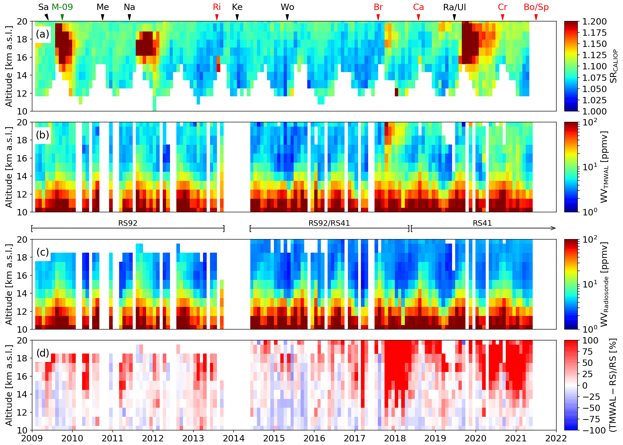
Figure 1 (a) Monthly and zonally averaged time series of aerosol scattering ratio derived from CALIOP between 2009 and the end of 2021 at 30–35^∘ N (Table Mountain Facility). Major eruptions (black triangles), PyroCb events (red triangles), and the MOHAVE-2009 (green triangle) field campaign are indicated at the top of the plot (see Table 1). (b) Monthly averaged TMWAL water vapor mixing ratio measurements during days where radiosonde launches were available. (c) Monthly averaged radiosonde water vapor mixing ratio. The periods where the RS92, RS92 and RS41, and RS41 radiosonde were used are indicated on top of the plot. (d) Relative difference between TMWAL and the radiosondes.

Table 1 Most significative volcanic eruptions (volcanic explosivity index (VEI) > 4) and PyroCb events affecting measurements over TMF, Payerne, and Reunion Island for the period comprehended between January 2009 and November 2022. Information regarding the location of the erupting volcanos and their VEI was retrieved from the Global Volcanism Program (https://volcano.si.edu/, last access: 22 November 2021). In the case of the PyroCbs, available references are included in the last column.

As mentioned in Sect. 1, there are many different systematic error sources affecting Raman lidar measurements, and each of them will have a specific way of affecting the retrievals, making them generally discernible from each other. In the case of aerosol extinction and insufficient blocking of Mie scattering, we would expect the impact on the measurements to be proportional to the intensity of the aerosol backscatter properties, regardless of the aerosol type (i.e., volcanic plumes, smoke plumes, dust, etc.). In case of fluorescence induced within the instrument optical components, we would expect a time-independent contamination, whether aerosols are present or not. On the other hand, in the case of fluorescence induced by the aerosols, we would expect a signature only in the presence of fluorescing aerosols.

When looking at the TMWAL and radiosonde time series, as well as the relative difference between the two presented in Fig. 1d, the most prominent disagreement appears towards the end of 2017 above 12 km a.s.l. This appears simultaneously with a strong increase in scattering ratio measured by CALIOP in a similar altitude range (Fig. 1a). This could suggest, in principle, insufficient blocking of the Mie scattering, but three other strong aerosol events observed by CALIOP around mid-2009, mid-2011, and the end of 2019 had a much larger scattering ratio, and yet the effect on the TMWAL water vapor profiles was negligible (Table 1). In particular, Leblanc et al. (2011) showed that measurements conducted during MOHAVE-2009 were simply unaffected by the aerosol plume from the Sarychev eruption. This suggests that the bias observed in TMWAL was associated with aerosol fluorescence rather than insufficient blocking of the elastic scattering. The three plumes, characterized by the largest scattering ratio and negligible impact on the TMWAL water vapor series, correspond to the eruption of the Sarychev, Nabro, and Ulawun/Raikoke volcanos (Khaykin et al., 2017). The plume observed at the end of 2017 corresponds to smoke aerosol particles injected into the lower stratosphere from a very notorious series of events, specifically five near-simultaneous intense PyroCbs (pyrocumulonimbus) occurring in western North America on 12 August 2017 (Peterson et al., 2018; Ansmann et al., 2018; Baars et al., 2019). At the end of 2018 and in 2019, this wet bias decreases significantly (observable down to 16 km a.s.l.), and then increases again in 2020 and 2021 as a result of further smoke injection associated with large PyroCbs registered in the western United States and Canada (NASA Earth Observatory, 2021). The present results are consistent with a case study previously reported by Immler et al. (2005), during which a Raman lidar located in Lindenberg (Germany) showed a water vapor wet bias inside a passing smoke plume that originated from wildfires in Portugal.

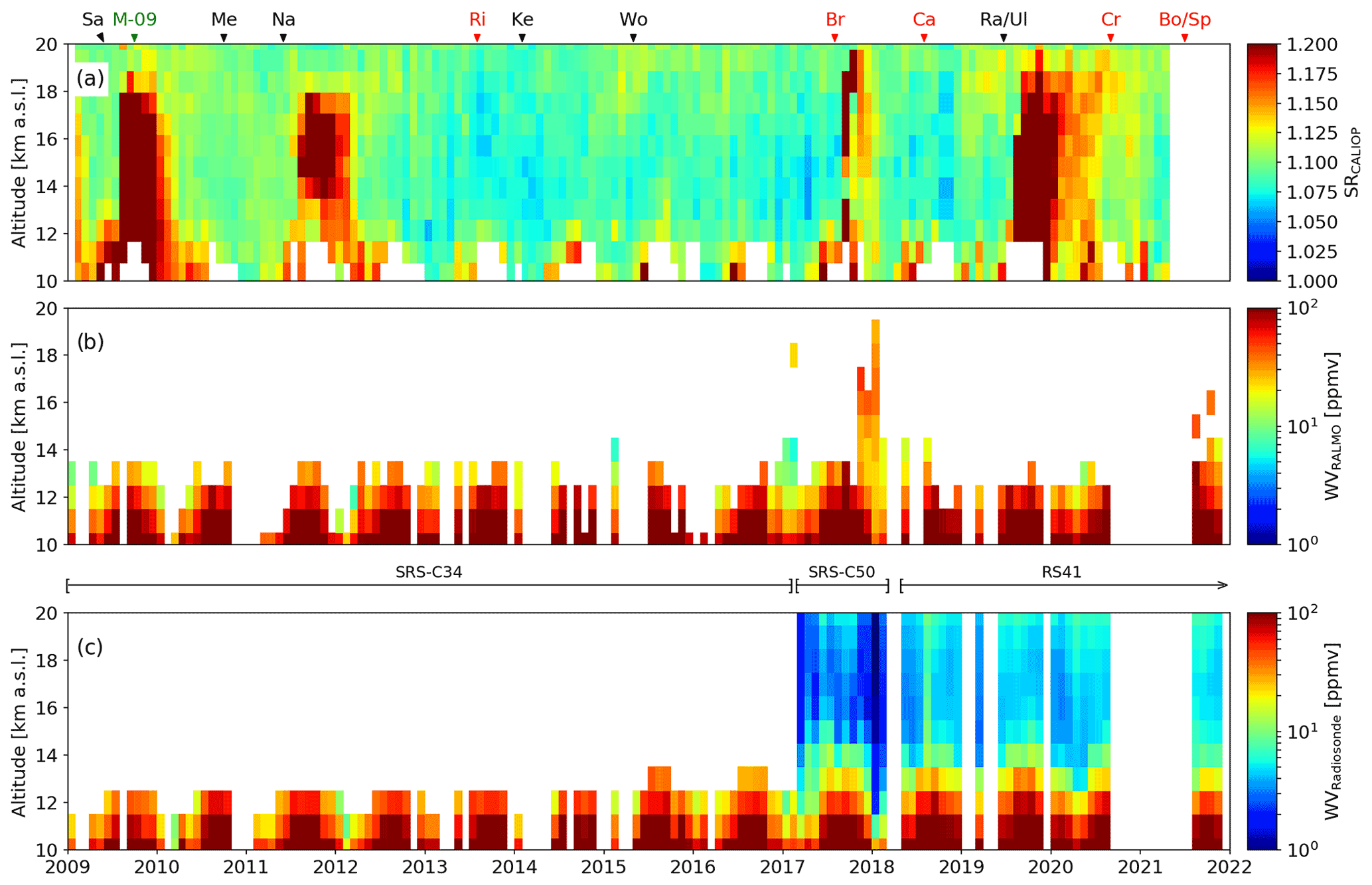
Figure 2 (a) Monthly and zonally averaged time series of aerosol scattering ratio derived from CALIOP between 2009 and the end of 2021 at 45–50^∘ N (Payerne). Major eruptions (black triangles), PyroCb events (red triangles), and the MOHAVE-2009 field campaign (green triangle) are indicated at the top of the plot (see Table 1). (b) Monthly averaged RALMO water vapor mixing ratio measurements during days where radiosonde launches were available. (c) Monthly averaged radiosonde water vapor mixing ratio. The periods where the SRS-C34, SRS-C50, and RS41 radiosondes were used are indicated on top of the plot.

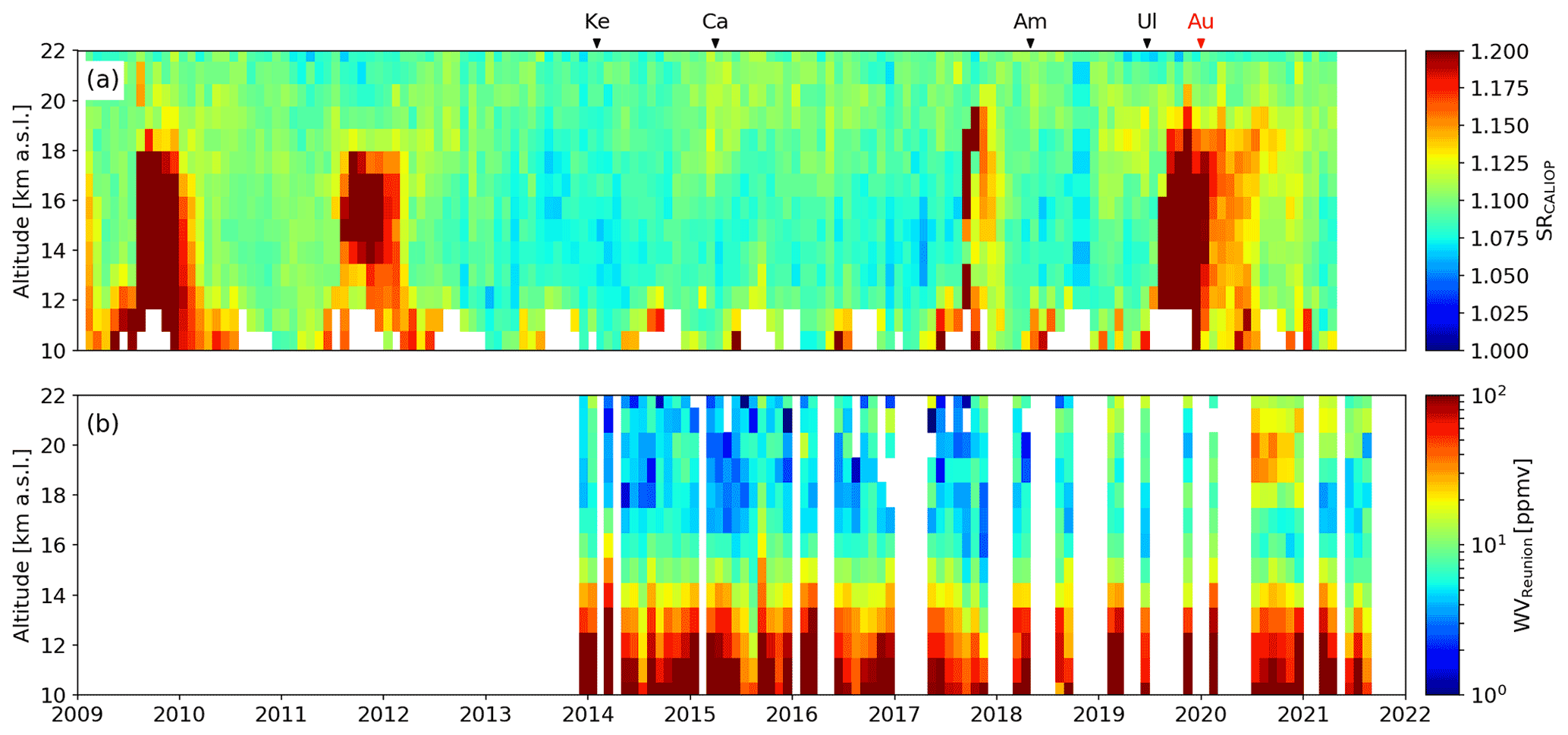
Figure 3 (a) Monthly and zonally averaged time series of aerosol scattering ratio derived from CALIOP between 2009 and the end of 2021 at 25–20^∘ S (Reunion Island). Major eruptions (black triangles) and PyroCb events (red triangle) are indicated at the top of the plot (see Table 1). (b) Monthly averaged Lidar1200 water vapor mixing ratio.

In order to further support our findings on the origin of the observed biases, we conducted a similar analysis on the RALMO (Fig. 2) and Lidar1200 (Fig. 3) lidar datasets. Because of the zonal symmetry and widespread nature of the volcanic and smoke plumes considered here in the northern hemispheric mid-latitudes, we expect the RALMO dataset to be influenced in a similar way to TMWAL's dataset. Although the uncertainty related to RALMO humidity measurements increases rapidly above 12–14 km a.s.l., we can clearly see an apparent positive bias in the lidar-measured water vapor towards the end of 2017 and the last months of 2021 (Fig. 2b) with respect to the co-located radiosoundings (Fig. 2c). Just like for TMWAL, the 2017 apparent wet bias is coincident with an increase of scattering ratio retrieved from CALIOP (Fig. 2a), which was traced back to the intense wildfires in British Columbia in summer 2017 (Peterson et al., 2018). This RALMO water vapor increase was not observed by the co-located Payerne radiosondes, which suggests again that this is the result of contamination of the water vapor lidar signal by fluorescing smoke. In fact, it is this enhancement of the water vapor signal by fluorescence what pushes the random uncertainty of the retrieval below the cutoff threshold. As in TMWAL, the RALMO water vapor dataset does not show any wet bias after the Raikoke/Ulawun eruption despite the large scattering ratio observed by CALIOP, confirming that insufficient blocking of Mie scattering by RALMO can be ruled out.

As for the Lidar1200 lidar at Reunion Island (southern hemispheric tropics), Fig. 3b exhibits the same behavior as for the other two lidars. There was no apparent impact of the Calbuco volcanic aerosol plume observed by CALIOP over Reunion Island during the 2015–2016 period. On the other hand, a strong apparent water vapor increase was observed by Lidar1200 during the second half of 2020 between 18 and 22 km a.s.l., an increase coinciding with the presence of the smoke plume produced by the January 2020 Australian fires. Although no radiosonde measurement is available at Reunion Island, the water vapor values observed by the lidar (> 40 ppmv) are unrealistically high, even considering the humidification of the UTLS caused by the smoke plume injection (Khaykin et al., 2020).

Based on the results presented in this section, we can conclude that fluorescence in smoke plumes transported in the UTLS induces substantial wet biases in the Raman lidar UV water vapor retrievals at different locations in the Northern and Southern Hemispheres. The wet biases remain as long as the fluorescing aerosols remain in the UTLS after their injection across the tropopause. It is important to point out that while large PyroCb events induce signatures in the water vapor lidar profiles that are easy to identify, smaller fire events produce smaller signatures that are more difficult to identify. Besides their reduced intensity, these events are more difficult to characterize, as the associated smoke plumes may have pathways that differ significantly from the typical deep convection induced by large fires. Smaller smoke injection events can potentially induce wet biases up to a few percent, very difficult to distinguish from other uncertainty sources and biases but large enough to affect the accuracy of trend detection. In an effort to minimize this impact, a correction technique relying on the addition of a dedicated “fluorescence channel” was developed. Details of this correction technique are presented in the following section.

4 Proposed correction

4.1 Method

In the typical Raman lidar UV water vapor technique, the emission wavelength is 355 nm and the water vapor signal is collected near 407.5 nm (Fig. 4), which corresponds to the Stokes Q-branch of the OH-stretching band (∼ 3654 cm⁻¹). In a dry clean atmosphere, most of the Raman-backscattered water vapor intensity is confined within ±0.5 nm of the strongest line, and after proper rejection of the much more intense elastic signal, the Raman water vapor signal is the only signal left between 406 and 410 nm. However, when the transmitted beam (355 nm) probes a layer of biogenic aerosol (smoke plume), an additional signal is produced, namely fluorescence, a broadband signal with a spectrum starting near the emission wavelength and extending well beyond the region of the Raman water vapor lines. In this case, the signal collected in the water vapor channel (407.5 nm) becomes the sum of the water vapor Raman backscatter signal and the fluorescence signal. The exact spectral shape of the fluorescence spectrum depends on the aerosol composition and is therefore typically unknown, with the exception that it is broadband, i.e., the spectrum varies slowly with wavelength and can thus be assumed to be nearly flat in the region 406–412 nm. Any deviation from this assumption will translate into a bias in the corrected water vapor. If fluorescence increases with wavelength, the correction will introduce a dry bias, while the opposite will happen in case of a fluorescence spectrum that decreases with wavelength. With these considerations in mind, we can design a new, dedicated “fluorescence channel”, the purpose of which is to estimate the intensity of fluorescence, and subtract it from the contaminated water vapor signal.

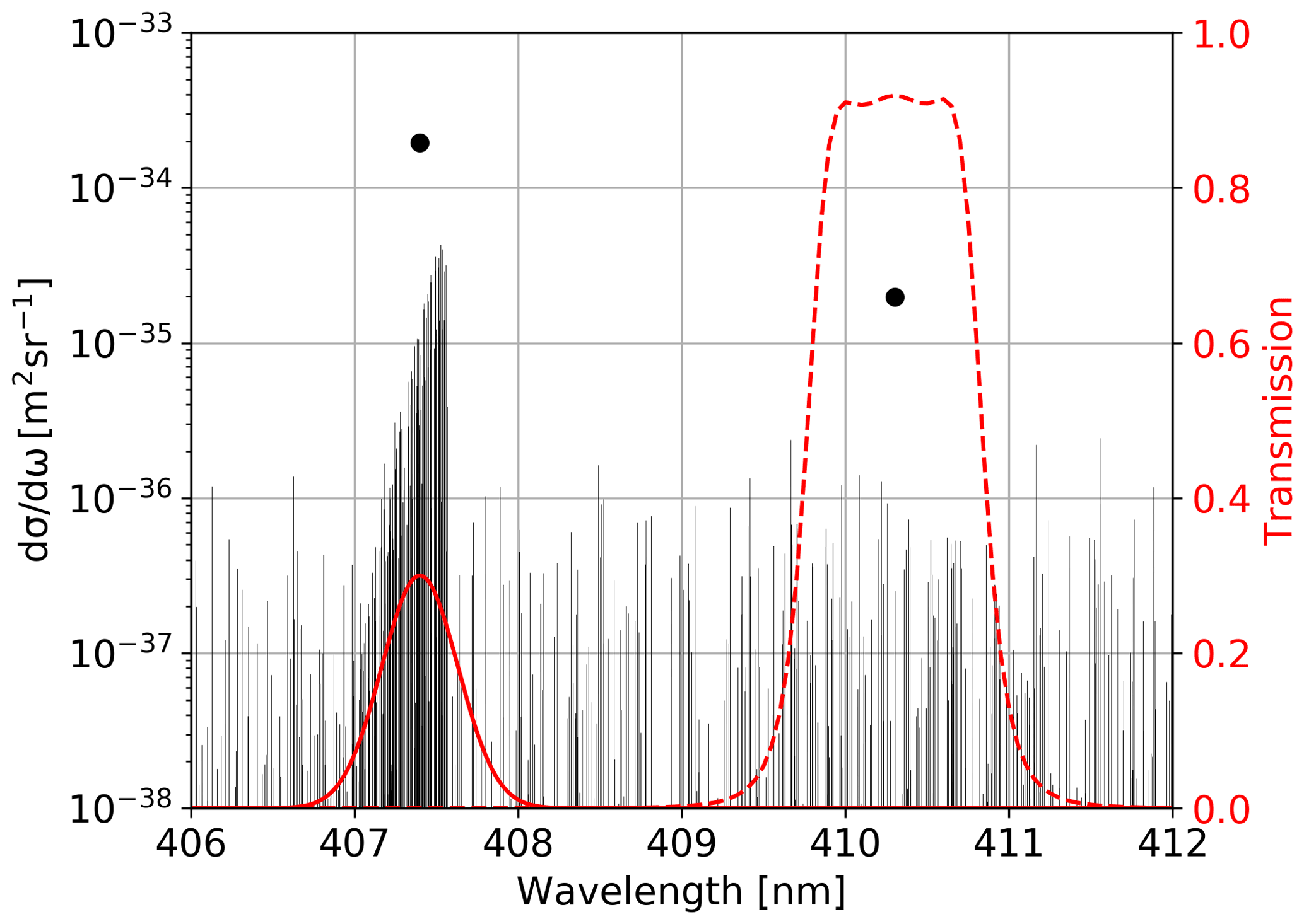
Figure 4 Water vapor Raman cross section spectrum (black lines) is shown together with the transmission of the water vapor channel filter (red line) and the new fluorescence-monitoring channel filter (dashed red line). The total water vapor Raman cross section for these two channels, as the result of integrating the product of the Raman cross section spectrum with the filter transmission of each channel between 406 and 412 nm, is also shown (black dots).

In an ideal scenario, we would like to have the water vapor and fluorescence channels set up so that they would each collect signal from their respective spectrum only. This is not possible because of the broadband nature of the fluorescence spectrum, so the idea is to pick a central wavelength for the fluorescence channel that is very close to the Raman water vapor lines, yet keeping the water vapor contribution as small as possible. We therefore selected a fluorescence filter with a central wavelength of 410.3 nm, a bandwidth of 1.1 nm FWHM (full width at half maximum), and a peak transmission of about 90 %. The central wavelength is less than 3 nm away from the central wavelength of the Raman water vapor channel, which allows us to assume a nearly identical magnitude of the fluorescence signal entering the water vapor and the fluorescence channels. This assumption seems to be reasonable based on several studies conducted on the fluorescence characteristics of biomass-burning aerosols, which show a broad slow-varying emission spectrum when biomass-burning aerosols are excited at 355 nm (e.g., Pan et al., 2007; Fu et al., 2015; Tang et al., 2020). At the same time, the intensity of the water vapor Raman scattering in the new fluorescence channel is attenuated by about an order of magnitude when compared to the Raman water vapor channel (Fig. 4).

The addition of the fluorescence channel had to be achieved with minimal disturbance to the existing receiver, and also at the lowest possible cost. Adding a dichroic beam splitter to keep the 407.5 nm on one end and add a new 410.3 nm channel on the other end was a possibility. However, the small spectral difference (3 nm) between the two channels would have made this option challenging, and the need for an additional photomultiplier tube (PMT) and its downstream electronics would have made this option less affordable. To reduce both cost and complexity, it was therefore decided to use a filter wheel instead. The new filter wheel is mounted in place of the original 407.4 nm interference filter, and now includes both the original filter at 407.4 nm and an additional 410.3 nm filter for the fluorescence data. The stability of the system is maximized, since the same 407.4 nm filter, same PMT, and same electronics are used for the water vapor channel. The new fluorescence channel actually uses the same hardware as the water vapor channel, except for the filter on the filter wheel. The data are acquired alternately for each filter as the wheel rotates through a pre-defined duty cycle. To minimize the effect of atmospheric variability between the acquisition of the water vapor and the fluorescence data, an interleaved acquisition scheme was implemented. Instead of the regular 2 h experiments, the results shown in Sect. 4.2 are the result of 4 h acquisitions, where the filter wheel is changed between the two filters every 30 min as part of our automated measurement routine.

Quantification of the fluorescence signal with respect to the water vapor signal is done not only by measuring the absolute signals in each channel, but also by inter-calibrating the two channels. The number of photons measured at a given range gate R on the Raman water vapor channel (N⁴⁰⁷) can be written as

$$\begin{array}{}\text{(1)}& N^{\mathrm{407}}\left(R\right)=N_{\mathrm{WV}}^{\mathrm{407}}\left(R\right)+N_{\mathrm{F}}^{\mathrm{407}}\left(R\right)+N_{\mathrm{BKG}}^{\mathrm{407}},\end{array}$$

where $N_{\mathrm{WV}}^{\mathrm{407}}$ represents the contribution from water vapor Raman scattering, $N_{\mathrm{F}}^{\mathrm{407}}$ represents fluorescence, and $N_{\mathrm{BKG}}^{\mathrm{407}}$ represents the background contribution (dominated by moonlight and sky background rather than PMT dark counts).

Similarly, the number of photons measured on the new fluorescence channel N⁴¹⁰ at the same range gate can be written in terms of the same components as

$$\begin{array}{}\text{(2)}& \begin{array}{rl}{N}^{\mathrm{410}}\left(R\right)& =k_{\mathrm{L}}^{\mathrm{407}\to \mathrm{410}}\cdot \left(k_{\mathrm{WV}}^{\mathrm{407}\to \mathrm{410}}\cdot N_{\mathrm{WV}}^{\mathrm{407}}\left(R\right)\right.\\ & \left.+k_{\mathrm{F}}^{\mathrm{407}\to \mathrm{410}}\cdot N_{\mathrm{F}}^{\mathrm{407}}\left(R\right)+k_{\mathrm{B}}^{\mathrm{407}\to \mathrm{410}}\cdot N_{\mathrm{BKG}}^{\mathrm{407}}\right)\end{array},\end{array}$$

where $k_{\mathrm{WV}}^{\mathrm{407}\to \mathrm{410}}$, $k_{\mathrm{F}}^{\mathrm{407}\to \mathrm{410}}$, and $k_{\mathrm{B}}^{\mathrm{407}\to \mathrm{410}}$ are proportionality constants given by the spectral characteristics of the Raman water vapor, fluorescence, and background signals, respectively. As mentioned before, we assume that the fluorescence spectra of the aerosols affecting the water vapor measurements can be considered to be constant over the 3 nm that separate the water vapor and the fluorescence-monitoring channels, making $k_{\mathrm{F}}^{\mathrm{407}\to \mathrm{410}}=\mathrm{1}$. On the other hand, $k_{\mathrm{L}}^{\mathrm{407}\to \mathrm{410}}$ is the lidar spectral response ratio and corresponds to the change in the lidar efficiency between these two wavelengths due to differences in filter transmission, filter width, PMT efficiency, etc. If we pick a range R_BKG where no water vapor or fluorescence contribution is expected ($N_{\mathrm{WV}}^{\mathrm{407}}\left(R_{\mathrm{BKG}}\right)=\mathrm{0}$ and $N_{\mathrm{F}}^{\mathrm{407}}\left(R_{\mathrm{BKG}}\right)=\mathrm{0}$), Eqs. (1) and (2) can be written as

$$\begin{array}{}\text{(3)}& N^{\mathrm{407}}\left(R_{\mathrm{BKG}}\right)=N_{\mathrm{BKG}}^{\mathrm{407}}\end{array}$$

and

$$\begin{array}{}\text{(4)}& N^{\mathrm{410}}\left(R_{\mathrm{BKG}}\right)=k_{\mathrm{L}}^{\mathrm{407}\to \mathrm{410}}\cdot k_{\mathrm{B}}^{\mathrm{407}\to \mathrm{410}}\cdot N_{\mathrm{BKG}}^{\mathrm{407}}.\end{array}$$

Since the wavelength difference between the N⁴⁰⁷ and N⁴¹⁰ channels is small, the background radiation at these two wavelengths is expected to be very close, and thus $k_{\mathrm{B}}^{\mathrm{407}\to \mathrm{410}}=\mathrm{1}$. In order to check this assumption, we retrieved the top-of-the-atmosphere (TOA) moonlight spectra based on the algorithm provided by Miller and Turner (2009). The 410/407 nm spectral ratio at the TOA is 1.03, and mostly independent of the moon phase. If we then assume that the atmospheric extinction is dominated by Rayleigh scattering around 400 nm (Cramer et al., 2013) and use a direct viewing geometry, we obtain $k_{\mathrm{B}}^{\mathrm{407}\to \mathrm{410}}=\mathrm{1.03}\cdot {\left(\frac{\mathrm{407}\mathrm{nm}}{\mathrm{410}\mathrm{nm}}\right)}^{\mathrm{4}}=\mathrm{1}$. While the direct moon viewing does not correspond to a real observation geometry, we expect the deviations from this assumption to be small based on other scattered moonlight model results (Jones et al., 2013).

Based on this assumption, we can derive our lidar spectral response ratio as

$$\begin{array}{}\text{(5)}& k_{\mathrm{L}}^{\mathrm{407}\to \mathrm{410}}={\displaystyle \frac{N^{\mathrm{410}}\left(R_{\mathrm{BKG}}\right)}{N^{\mathrm{407}}\left(R_{\mathrm{BKG}}\right)}}.\end{array}$$

Because $k_{\mathrm{L}}^{\mathrm{407}\to \mathrm{410}}$ is related to the characteristics of the lidar components, we expect it to remain mostly constant over time, as long as there is no change in the lidar setup. Also, as mentioned before, this calculation assumes that the background signals are dominated by moonlight sky background and that the contribution of the PMT dark counts and other light sources with unknown spectral characteristics is negligible. In order to verify this assumption, we analyzed the stability of the ratio defined in Eq. (5) as a function of the background levels.

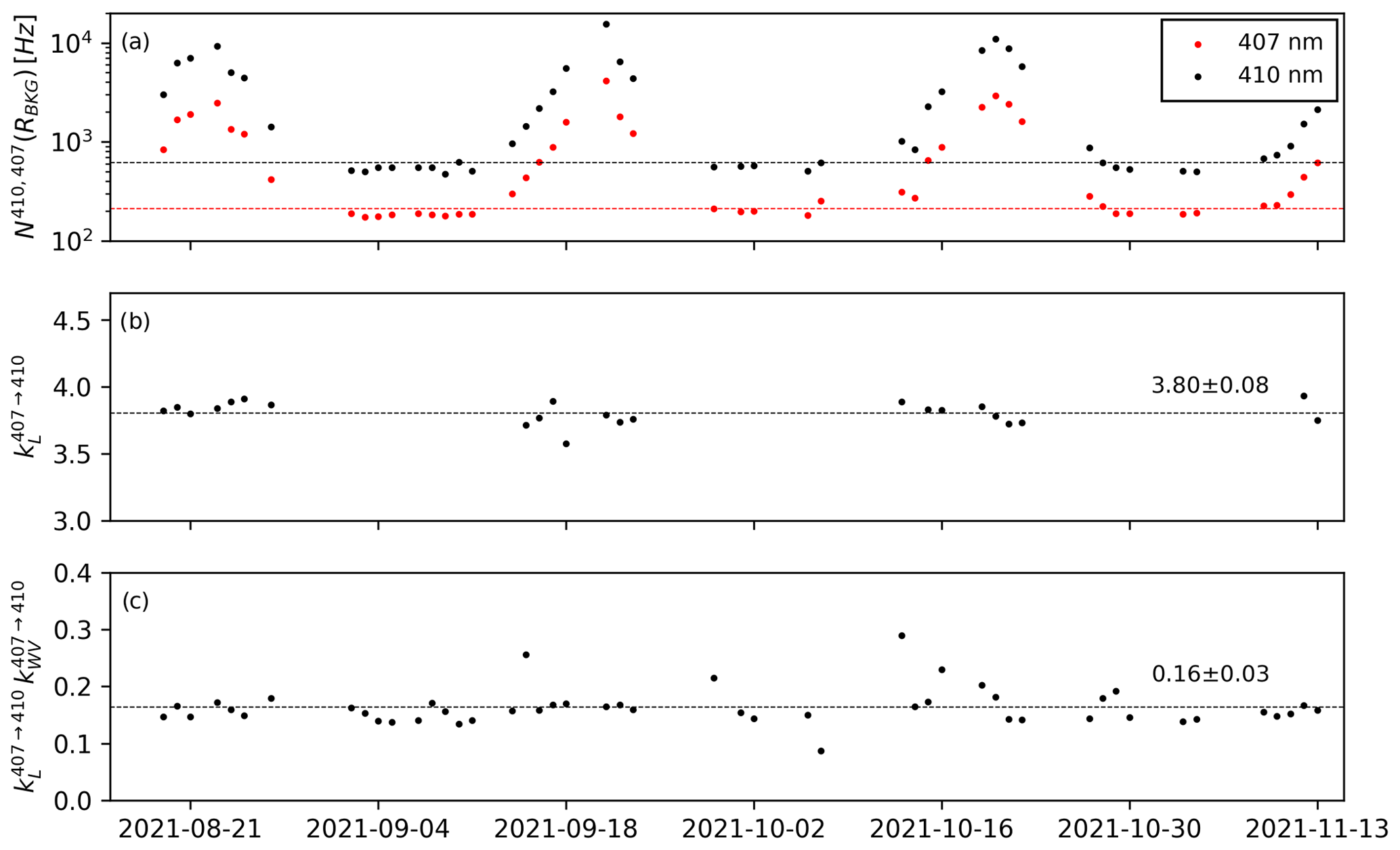
Figure 5 (a) Time series of background levels for the 407 nm (red dots) and 410 nm (black dots) channels. The average of the background levels for days where other unknown light sources dominate (low moonlight contribution) is also shown (dashed red and dashed black lines). (b) Time series of the 410/407 nm channel background ratio (lidar spectral response ratio) calculated based on days where moonlight dominates and after subtracting the contribution from unknown light sources. The average of the lidar spectral response ratio is also shown (dashed black line). (c) Time series of the ratio between the 410/407 nm channels for altitudes between 9–11 km a.s.l., where the fluorescence contribution can be typically considered negligible (Eq. 6). The average is also shown (dashed black line).

The background levels presented in Fig. 5a show a clear temporal pattern caused by the moon phases, with a maximum background occurring during the full moon phase. As the moon illumination drops towards new moon, we can see that the background levels stabilize to relatively constant values, while maintaining a substantial difference between the 407 and 410 nm channels. Since these two channels share the same PMT and optical path (with the exception of a changing filter), we can conclude that these background levels are not related to PMT dark counts but rather to a different background source (i.e., light pollution from the Los Angeles basin and other nearby sources). Since the calculation of $k_{\mathrm{L}}^{\mathrm{407}\to \mathrm{410}}$ assumes knowledge of the background spectral characteristics, we first estimated the contribution of the light pollution as the average of the background for days where the moonlight contribution is negligible (Fig. 5a). This average was then subtracted from the background levels of moon-dominated days in order to keep only the moonlight contribution, which has a known spectrum. The ratio of these two channels after correction (Fig. 5b) exhibit a fairly constant value, with an average of 3.8 ± 0.08.

Next, the constant term $k_{\mathrm{WV}}^{\mathrm{407}\to \mathrm{410}}$ can be determined by calculating the ratio of the 407 and 410 nm signals (after background subtraction) for a range R at which the fluorescence contribution is negligible, or else using laboratory measurements of the water vapor Raman spectrum. From Eqs. (1) and (2), after background subtraction (denoted by *), and assuming $N_{\mathrm{F}}^{\mathrm{407}}\left(R\right)\ll N_{\mathrm{WV}}^{\mathrm{407}}\left(R\right)$,

$$\begin{array}{}\text{(6)}& k_{\mathrm{L}}^{\mathrm{407}\to \mathrm{410}}\cdot k_{\mathrm{WV}}^{\mathrm{407}\to \mathrm{410}}={\displaystyle \frac{N^{\mathrm{410}\ast }\left(R\right)}{N^{\mathrm{407}\ast }\left(R\right)}}.\end{array}$$

Figure 5c shows the result of applying Eq. (6) to each measurement period between 9 and 11 km a.s.l., where $N_{\mathrm{F}}^{\mathrm{407}}\left(R\right)\ll N_{\mathrm{WV}}^{\mathrm{407}}\left(R\right)$. This ratio shows a relatively stable behavior and a mean value of 0.16 ± 0.03, which translates into $k_{\mathrm{WV}}^{\mathrm{407}\to \mathrm{410}}=\mathrm{0.042}$. This result is relatively close to the one obtained by the other proposed method (laboratory measurements of the water vapor Raman cross-section) and shown in Fig. 4 as the two black dots with a ratio of about 0.1. The difference between these two approaches can be attributed to several different factors not accounted for in the calculation, like departure of the filter transfer functions from the values used for the calculation, changes in the PMT response function between the two wavelengths, etc.

After background subtraction we have the following equation system, where we can obtain the fluorescence-corrected water vapor signal needed to conduct the standard Raman lidar water vapor retrieval:

$$\begin{array}{}\text{(7)}& N^{\mathrm{407}\ast }\left(R\right)=N_{\mathrm{WV}}^{\mathrm{407}}\left(R\right)+N_{\mathrm{F}}^{\mathrm{407}}\left(R\right)\end{array}$$

and

$$\begin{array}{}\text{(8)}& \begin{array}{rl}{N}^{\mathrm{410}\ast }\left(R\right)& =k_{\mathrm{L}}^{\mathrm{407}\to \mathrm{410}}\cdot k_{\mathrm{WV}}^{\mathrm{407}\to \mathrm{410}}\cdot N_{\mathrm{WV}}^{\mathrm{407}}\left(R\right)\\ & +k_{\mathrm{L}}^{\mathrm{407}\to \mathrm{410}}\cdot N_{\mathrm{F}}^{\mathrm{407}}\left(R\right)\end{array}.\end{array}$$

From Eq. (7),

$$\begin{array}{}\text{(9)}& N_{\mathrm{WV}}^{\mathrm{407}}\left(R\right)=N^{\mathrm{407}\ast }\left(R\right)-N_{\mathrm{F}}^{\mathrm{407}}\left(R\right),\end{array}$$

while from Eq. (8),

$$\begin{array}{}\text{(10)}& N_{\mathrm{F}}^{\mathrm{407}}\left(R\right)={\displaystyle \frac{\mathrm{1}}{k_{\mathrm{L}}^{\mathrm{407}\to \mathrm{410}}}}{N}^{\mathrm{410}\ast }\left(R\right)-k_{\mathrm{WV}}^{\mathrm{407}\to \mathrm{410}}\cdot N_{\mathrm{WV}}^{\mathrm{407}}\left(R\right).\end{array}$$

Replacing Eq. (10) in Eq. (9), we obtain an expression of the “true” water vapor contribution (i.e., the corrected water vapor profile), $N_{\mathrm{WV}}^{\mathrm{407}}\left(R\right)$:

$$\begin{array}{}\text{(11)}& N_{\mathrm{WV}}^{\mathrm{407}}\left(R\right)={\displaystyle \frac{N^{\mathrm{407}\ast }\left(R\right)}{\left(\mathrm{1}-k_{\mathrm{WV}}^{\mathrm{407}\to \mathrm{410}}\right)}}-{\displaystyle \frac{N^{\mathrm{410}\ast }\left(R\right)}{k_{\mathrm{L}}^{\mathrm{407}\to \mathrm{410}}\left(\mathrm{1}-k_{\mathrm{WV}}^{\mathrm{407}\to \mathrm{410}}\right)}}.\end{array}$$

4.2 Correction results and uncertainty

To evaluate the performance of the fluorescence correction method described in the previous section, we conducted a series of 22 experiments at JPL-TMF between 27 August and 4 November 2021, where the uncorrected and corrected TMWAL profiles were compared with co-located RS41 radiosonde launches. The results of these tests are summarized in Fig. 6.

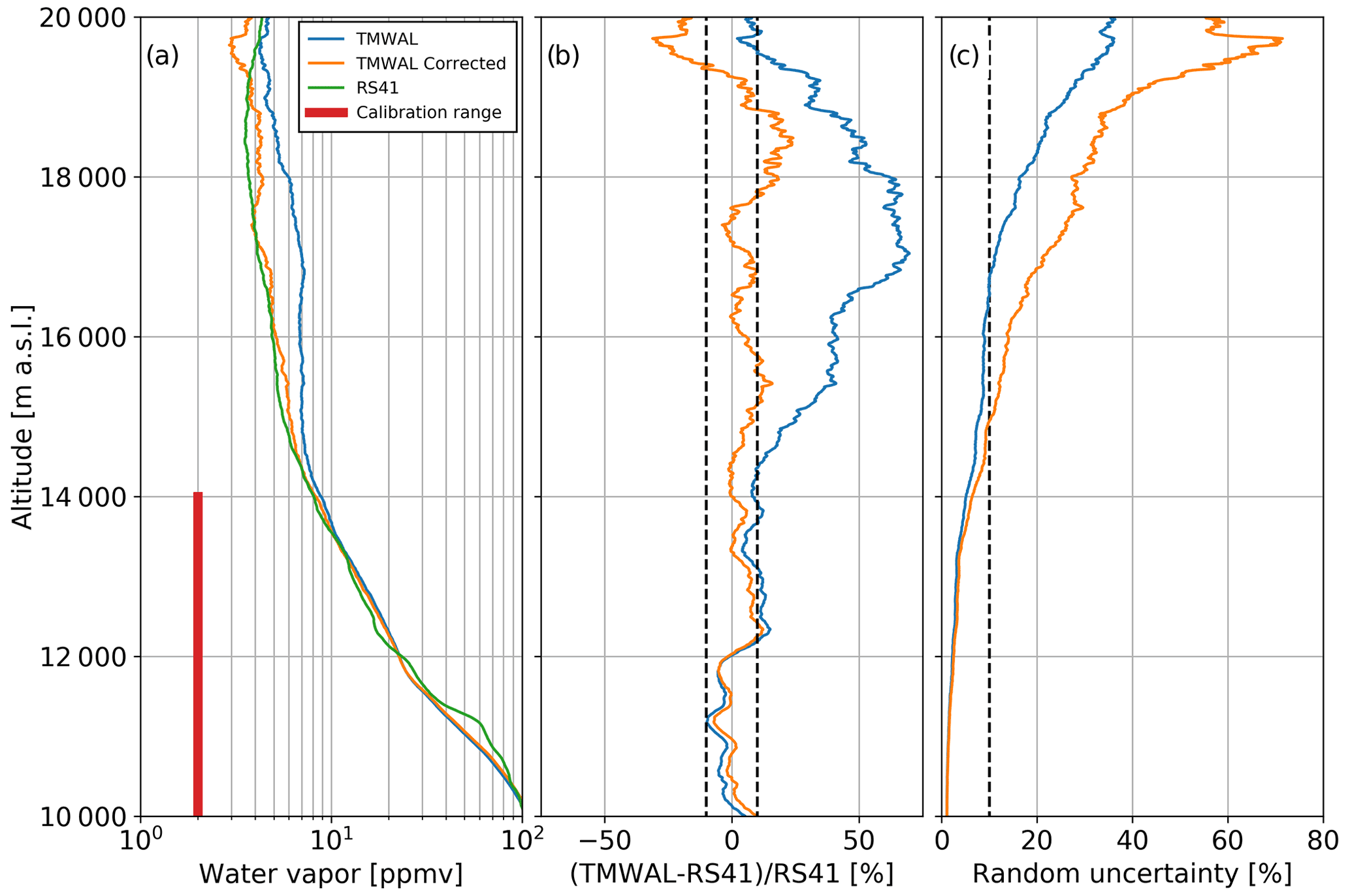
Figure 6 (a) The average of the 22 profiles measured between 27 August and 4 November 2021 by TMWAL before the correction method was applied (solid blue line) and after the correction method was applied (solid orange line) are shown together with the average of the co-located RS41 radiosonde profiles (solid green line). The retrieved TMWAL profiles are calibrated using the RS41 measurements between 9 and 14 km a.s.l. (red stripe). (b) Average of the relative difference between the uncorrected (solid blue line) and corrected (solid orange line) TMWAL profiles when compared with the co-located RS41 launches. (c) Average random uncertainty (1σ) for the uncorrected (solid blue line) and corrected (solid orange line) TMWAL profiles.

Between 14 and 20 km a.s.l., the average of the uncorrected TMWAL profiles (blue curve) shows a clear wet bias (> 50 %) with respect to the RS41 mean profile, reaching a maximum of 75 % between 17 and 18 km a.s.l. This is similar to the biases observed before the correction method was implemented towards the end of August 2021 (Fig. 1d). The average of the corrected profiles (orange curve) shows a much better agreement with the RS41 mean profile, within 10 % for most of the altitudes and within 5 % overall. Above 18 km a.s.l., the difference to the RS41 increases to about 25 %. Above 19.3 km a.s.l., the corrected profile gets drier than the RS41 profile, but the low signal-to-noise ratio at these altitudes makes the difference clearly statistically not significant. When only profiles measured during low background conditions (new moon) are used, this deviation at the top of the profile is substantially reduced (not shown).

The main factor controlling the performance of the proposed correction method is the accuracy in the determination of the $k_{\mathrm{L}}^{\mathrm{407}\to \mathrm{410}}$ and $k_{\mathrm{F}}^{\mathrm{407}\to \mathrm{410}}$ constants. These two constants have a similar impact on the final result, but $k_{\mathrm{F}}^{\mathrm{407}\to \mathrm{410}}$ is substantially more difficult to quantify and much more variable, as it depends on the composition of the interfering aerosols.

The next consideration is the expected increase in the corrected water vapor random uncertainty. The Raman lidar technique uses the ratio of signals backscattered by water vapor and nitrogen. In the UTLS, the random noise is dominated by the water vapor channel detection noise, since the nitrogen signal is several orders of magnitude larger than the water vapor signal. With the assumption that the water vapor and fluorescence components are independent, the variance of the corrected water vapor signal is the sum of the original water vapor signal variance and the fluorescence signal variance divided by the lidar spectral response ratio. At altitudes above 16 km, where the fluorescence signal is of the same order of magnitude as the water vapor signal, we expect a substantial increase in the random uncertainty of the corrected retrieval. In order to verify this, we conducted a Monte Carlo (MC) simulation. The MC uncertainty simulation presented in Fig. 6c is the result of 100 realizations, where each realization models all contributing uncertainties (calibrations and detection noise) as normally distributed. While the detection noise of each individual detected shot follows a Poisson distribution, the average detection noise of each experiment (realization) can be modeled as normally distributed following the central limit theorem. Figure 6c shows that the random uncertainty of the corrected TMWAL profiles is about 50 % larger than that of the uncorrected profiles over the altitude range where the correction is most important. The increase in the random uncertainty affects the ability of the system to detect potential trends (Whiteman et al., 2011), and additional measurements would typically be required to mitigate this degradation. However, the systematic uncertainty introduced by the fluorescence correction (determination of $k_{\mathrm{L}}^{\mathrm{407}\to \mathrm{410}}$ and $k_{\mathrm{F}}^{\mathrm{407}\to \mathrm{410}}$ constants) remains the most critical component for accurate estimation of long-term trends.

5 Discussion and conclusions

Almost two decades after being added to the suite of NDACC instrumentation, the water vapor Raman lidar technique is facing a new, unforeseen challenge with the recent increase of lower stratospheric aerosol loading. In the Northern Hemisphere, sustained droughts in North America and Siberia have been responsible for large and more frequent wildfires since 2017. Many of these fires led to substantial PyroCb events, resulting in the injection of unprecedented quantities of smoke into the northern hemispheric lower stratosphere. Large injections of smoke also occurred in the southern hemispheric lower stratosphere following the Australian wildfires in the austral summer 2019/2020. It has been shown that the smoke plumes originating from these fires are subject to self-lofting, which enhances their vertical development over time (Ohneiser et al., 2022). When smoke layers in the UTLS are sounded by water vapor Raman lidars transmitting in the UV range (355 nm), they fluoresce and can cause significant contamination of the weak water vapor lidar signals collected at these altitudes. Such contamination was identified in the present study using the long-term water vapor datasets of three ground-based UV water vapor Raman lidars contributing to NDACC, together with the aerosol scattering ratio profiles from the spaceborne CALIOP lidar. Between 2009 and 2017, no large wildfire event was identified, and only volcanic eruptions caused observable injection of aerosols in the stratosphere. Over this period, the TMWAL lidar was able to provide excellent-quality water vapor profiles, typically up to 20 km. However, since 2017, the impact of the increased wildfire activity on TMWAL, RALMO, and Lidar1200 water vapor data was clearly identified in the UTLS, with a high bias of up to 75 % at 17 km for TMWAL. As a result of this contamination, a large fraction of the TMWAL water profiles had to be cut-off below 15 km before they were archived at NDACC.

As of today, it is difficult to predict if this increased fire activity is temporary, or if it will become the norm for the next decades. In any case, it has raised the important question of the usefulness of UV Raman lidar water vapor measurements for the detection of long-term trends in the UTLS. Our present study shows that a low-cost upgrade of the lidar receiver allows for a fluorescence correction. Our results are encouraging, and allowed us to basically remove the fluorescence contribution from the contaminated lidar signals. The improvement results in a drastic reduction of the water vapor wet bias (up to 75 % between 17 and 18 km a.s.l.), leading to a difference of only 5 % with our co-located radiosonde measurements. However, this correction was possible at the cost of increasing the total uncertainty, making the accurate detection of trends in the UTLS questionable. Using the TMWAL data, it is shown that the relative impact of the fluorescence increases abruptly at around 15 km (Fig. 6b). It is therefore reasonable to think that the detection of long-term water vapor trends by UV Raman lidars will only be slightly impacted in the upper troposphere where the water vapor mixing ratio is larger than 20 ppmv, but will likely be very challenging in the lower stratosphere without implementing very accurate fluorescence-correction techniques.

The next question is therefore to establish whether a different lidar configuration can lead to more robust water vapor measurement in the UTLS. Different alternatives have been evaluated. One option is to add a second fluorescence channel with a central wavelength slightly lower than the existing Raman water vapor channel. By doing so, there is the potential to reduce the uncertainty in the shape of the fluorescence spectrum in the region of the Raman water vapor lines. This better quantitative estimation of fluorescence will reduce the correction uncertainty and, therefore, total uncertainty in the corrected water vapor. Another option is to add a second water vapor channel using a filter of broader bandwidth. This option, however, would make the retrieval more sensitive to variability in k_w, as both channels will have a similar contribution of water vapor Raman scattering. Another possible but much more expensive option is the addition of a spectrometer. This type of instrumentation allows, in principle, an accurate quantitative estimation of the fluorescence spectrum in the entire 406–412 nm region, and once again would reduce the corrected water vapor uncertainty.

Unfortunately, none of the lidar receiver upgrades just proposed provides the certainty to drastically improve water vapor measurement in the UTLS. As an alternative to implementing a fluorescence correction, modification of TMWAL to operate at a different wavelength is now considered. Although not negligible, aerosol fluorescence in the UTLS is expected to be much lower when the aerosol layer is excited at 532 nm. Using the YAG second harmonic would increase the transmitted power by a factor of two, but the wavelength dependence of the Raman and Rayleigh scattering, the generally lower performance of PMTs in that spectral region, and the expected higher sky background noise would ultimately result in a reduction of the signal-to-noise ratio by a factor of about two (Sherlock et al., 1999) compared to our UV (355 nm) transmitter. This option has significant potential, but its implementation at JPL-TMF is expected to be costly and time consuming. Meanwhile, several NDACC Raman lidars currently operate at 532 nm. Alternatively, we are also evaluating the possibility of using a XeCl excimer laser (308 nm) as the source (Klanner et al., 2021). While generally speaking, a larger impact of aerosol fluorescence is expected when operating at shorter wavelengths, this is not necessarily true for the type of components responsible for the observed fluorescence interference in the UTLS. Benzo[a]pyrene, one of the components typically found in smoke and mentioned by Immler et al. (2005) as potentially responsible for the observed fluorescence contamination, exhibits very little emission below 350 nm (Fernández-Sánchez et al., 2003). While such a system would profit from stronger Raman backscatter and lower sky background as compared to the YAG second harmonic alternative, it might have a stronger interference with ozone and other types of atmospheric aerosols.

An increased scrutiny of the performance of these alternative transmission wavelengths in the UTLS is being called for. Discussion within the NDACC community was initiated, with the main objective to foster close collaboration with key NDACC water vapor lidar groups using a transmitter at 532 nm or 308 nm and to assess the sensitivity of these lidars to aerosol fluorescence in the UTLS. Once this assessment is complete and successful, the scientific community in general, and the NDACC community in particular, will need to make important decisions regarding the UTLS long-term water vapor measurement strategy for the upcoming decades.