the Creative Commons Attribution 4.0 License.
the Creative Commons Attribution 4.0 License.
 | 29 Jul 2022
Synergetic use of IASI profile and TROPOMI total-column level 2 methane retrieval products
Matthias Schneider
Benjamin Ertl
Qiansi Tu
Christopher J. Diekmann
Farahnaz Khosrawi
Amelie N. Röhling
Frank Hase
Darko Dubravica
Omaira E. García
Eliezer Sepúlveda
Tobias Borsdorff
Jochen Landgraf
Alba Lorente
André Butz
Huilin Chen
Rigel Kivi
Thomas Laemmel
Michel Ramonet
Cyril Crevoisier
Jérome Pernin
Martin Steinbacher
Frank Meinhardt
Kimberly Strong
Debra Wunch
Thorsten Warneke
Coleen Roehl
Paul O. Wennberg
Isamu Morino
Laura T. Iraci
Kei Shiomi
Nicholas M. Deutscher
David W. T. Griffith
Voltaire A. Velazco
David F. Pollard
The thermal infrared nadir spectra of IASI (Infrared Atmospheric Sounding Interferometer) are successfully used for retrievals of different atmospheric trace gas profiles. However, these retrievals offer generally reduced information about the lowermost tropospheric layer due to the lack of thermal contrast close to the surface. Spectra of scattered solar radiation observed in the near-infrared and/or shortwave infrared, for instance by TROPOMI (TROPOspheric Monitoring Instrument), offer higher sensitivity near the ground and are used for the retrieval of total-column-averaged mixing ratios of a variety of atmospheric trace gases. Here we present a method for the synergetic use of IASI profile and TROPOMI total-column level 2 retrieval products. Our method uses the output of the individual retrievals and consists of linear algebra a posteriori calculations (i.e. calculation after the individual retrievals). We show that this approach has strong theoretical similarities to applying the spectra of the different sensors together in a single retrieval procedure but with the substantial advantage of being applicable to data generated with different individual retrieval processors, of being very time efficient, and of directly benefiting from the high quality and most recent improvements of the individual retrieval processors.
We demonstrate the method exemplarily for atmospheric methane (CH4). We perform a theoretical evaluation and show that the a posteriori combination method yields a total-column-averaged CH4 product (XCH4) that conserves the good sensitivity of the corresponding TROPOMI product while merging it with the high-quality upper troposphere–lower stratosphere (UTLS) CH4 partial-column information of the corresponding IASI product. As a consequence, the combined product offers additional sensitivity for the tropospheric CH4 partial column, which is not provided by the individual TROPOMI nor the individual IASI product. The theoretically predicted synergetic effect is verified by comparisons to CH4 reference data obtained from collocated XCH4 measurements at 14 globally distributed TCCON (Total Carbon Column Observing Network) stations, CH4 profile measurements made by 36 individual AirCore soundings, and tropospheric CH4 data derived from continuous ground-based in situ observations made at two nearby Global Atmospheric Watch (GAW) mountain stations. The comparisons clearly demonstrate that the combined product can reliably detect the actual variations of atmospheric XCH4, CH4 in the UTLS, and CH4 in the troposphere. A similar good reliability for the latter is not achievable by the individual TROPOMI and IASI products.
- Article
(13977 KB) - Full-text XML
- Comment
- BibTeX
- EndNote


Measurements from different ground- or satellite-based sensors target at the observations of the same atmospheric parameters (e.g. the same trace gases) but with different characteristics (e.g. sensitivities for different vertical regions). Often the different sensors use different observation geometries (limb scanning, nadir, solar light reflected at the Earth's surface) and/or different spectral regions (e.g. UV–Vis, near-infrared, thermal infrared, and microwave). Dedicated experts and efforts are needed to develop retrieval techniques that are specifically optimized for an individual sensor. An algorithm that uses coincident measurements of all the different sensors for a multispectral approach (synergetic use of level 1 data) for the optimal estimation of the atmospheric state would exploit the synergies of the different observation geometries and spectral regions well and thus allows for detection of the atmospheric state in more detail than is achievable by individual optimal estimation retrievals.
There is a variety of studies investigating the multispectral synergism when retrieving atmospheric trace gases from space. Examples of theoretical studies using synthetic thermal infrared and UV spectra for a simulated synergistic retrieval of atmospheric ozone (O3) are Landgraf and Hasekamp (2007), Worden et al. (2007), Cuesta et al. (2013), and Costantino et al. (2017). These studies considered the thermal infrared spectra of TES (Tropospheric Emission Spectrometer) and IASI (Infrared Atmospheric Sounding Interferometer as well as its successor IASI – New Generation) and UV spectra of OMI (Ozone Monitoring Instrument) and GOME-2 (Global Ozone Monitoring Experiment – 2 as well as its successor UVNS – Ultraviolet Visible Near-infrared Shortwave-infrared) and are complemented by studies with real spectra (e.g. Cuesta et al., 2013; Fu et al., 2013). Another example of a study with real spectra is Luo et al. (2013), who examine the combination of the TES thermal nadir spectra with the MLS (Microwave Limb Sounder) microwave limb spectra for a synergetic retrieval of atmospheric carbon monoxide (CO) profiles. All the different studies clearly show that the synergetic use of the measured spectra results in an increased sensitivity with respect to the targeted trace gases.
However, the development of these multispectral retrievals requires experts in different remote-sensing techniques to work closely together. Furthermore, as soon as measurements from a new sensor become available (or as soon as sensors are modified/improved), such multispectral processors have to be adapted accordingly; i.e. continuous collaborative retrieval developments are required. While this is certainly possible, it might not be the most efficient way, in particular considering the steadily increasing number of available satellite data products (level 2 retrieval products). The optimal synergetic exploitation of the level 2 retrieval products that are already available would be much less computationally expensive than running dedicated multispectral retrievals. Such synergetic combination of level 2 products is the topic of this paper.
There are already several examples of a level 2 product fusion discussed in literature (the following list is not intended to be complete): Worden et al. (2015) combine the thermal and near-infrared level 2 products of methane (CH4) of TES and GOSAT (Greenhouse gas mOnitoring SATellite), respectively, by performing approximative calculations and with a focus on monthly mean data. Data aggregation is necessary due to the reduced temporal and horizonal coverage of TES and GOSAT and their imperfect collocation. Cortesi et al. (2016) combine the thermal infrared MIPAS-STR (Michelson Interferometer for Passive Atmospheric Sounding – STRatospheric aircraft) and microwave MARSCHALS (Millimetre-wave Airborne Receivers for Spectroscopic Characterization in Atmospheric Limb Sounding) aircraft-based remote-sensing products of O3, nitric acid (HNO3), water vapour (H2O), and atmospheric temperature (applying the so-called “measurement-space solution” data fusion method of Ceccherini et al., 2009). Another example is Warner et al. (2014), who use a Kalman filter for combining the CO data products of AIRS (Atmospheric Infrared Sounder) – available for a large horizontal area but with weak vertical details – and TES (and MLS) – available with detailed vertical information but only for very localized areas.
Here, we present a method for fusing the available level 2 CH4 profile product of IASI and the XCH4 (total-column-averaged methane) product of TROPOMI (Tropospheric Monitoring Instrument) by means of a Kalman filter approach. Our objective is a data product with improved vertical profile information (determine tropospheric CH4 independently from CH4 at higher altitudes, which is not possible by IASI or TROPOMI data alone) by synergetically exploiting the different vertical sensitivities of the two products.
The method allows for a computationally very efficient generation of global daily maps of the combined data product and only needs the individually retrieved states, averaging kernels, and noise covariances provided by the respective remote-sensing experts in the context of their standard retrieval work. The proposed method can be used flexibly for combining measurement information of different satellite sensors and is in particular interesting for combining a profile product with a total-column product. The method has strong theoretical similarities to a dedicated combined optimal estimation retrieval that uses the combined IASI and TROPOMI spectra as input (synergetic use of level 1 data).
The reliable and global detection of tropospheric CH4 independently from CH4 at higher altitudes can lead to an improved understanding of the CH4 cycle. Respective data allow for a more direct investigation of the CH4 boundary layer source and sink signals than total-column-averaged mixing ratios (XCH4) provided globally for instance by GOSAT (e.g. Parker et al., 2020) or TROPOMI (Lorente et al., 2021a). This is because XCH4 signals are strongly affected by vertical shifts of the tropopause altitude; i.e. their use for investigating CH4 absorption and release at the ground depends on the correct consideration of the tropopause altitude by model simulations (Pandey et al., 2016).
This paper is organized as follows. Section 2 briefly presents the used IASI and TROPOMI products (generated by two individual retrievals). Section 3 presents the equations for the optimal a posteriori combination of the two independent retrieval outputs (level 2 product combination) and performs a theoretical evaluation of the individual and combined products. Section 4 validates the total- column and tropospheric and UTLS (upper troposphere–lower stratosphere) partial-column products obtained by the individual IASI and TROPOMI retrievals and by the a posteriori combination by an inter-comparison to reference data from the Total Carbon Column Observing Network (TCCON), AirCore, and Global Atmospheric Watch (GAW). Section 5 discusses the global consistency of the products and shows global maps. Section 6 resumes the results of our study and briefly discusses upcoming possibilities. Furthermore, in Appendix A we give a brief overview on retrieval theory, and in Appendix B we discuss the theory of our a posteriori combination method and show that the method has strong similarities to performing a full multispectral optimal estimation retrieval. Appendix C introduces the operator for transferring logarithmic-scale differentials into linear-scale differentials. Appendix D presents the operators used for converting vertical profile data into total- and partial-column data. Appendix E examines the dislocation error, i.e. to what extent the temporal and spatial dislocation of the IASI and TROPOMI observations (the two sensors are on two different satellites with different orbits) impacts the combined data product. Appendix F explains how we assess the comparability of the satellite products with the reference data and reveals the reasonable agreement between the characteristics of the satellite products and the results of the validation study.
In this section we briefly present the satellite data products that are used for the combination procedure. These are the XCH4 data obtained from the analysis of the near-infrared and shortwave infrared (SWIR and NIR) spectra measured by TROPOMI and the CH4 profiles derived from IASI thermal nadir (TIR) spectra. In addition, we explain the criteria used for collocating the two satellite observations.
2.1 RemoTeC TROPOMI XCH4
The TROPOMI XCH4 data used in this study are generated by the RemoTeC algorithm (Butz et al., 2011), which is used for the operational processing of Sentinel 5 Precursor/TROPOMI XCH4 data (Hu et al., 2016; Hasekamp et al., 2021). Here we work with data of the operational processing algorithm version 2.2.0 (which has been presented and validated in Lorente et al., 2021a). The TROPOMI output files provide the XCH4 data together with the a priori data used (constructed from simulations of the global chemistry-transport model TM5; Krol et al., 2005), the column averaging kernels, and the error values. Here we work with all TROPOMI data that pass the standard quality filtering (TROPOMI output variable qa_value must be equal to 1.0, which means a filtering according to Table A1 of Lorente et al., 2021a). In addition, we remove observations over ground covered by snow (which show a high bias as discussed in Lorente et al., 2021a) by requiring a blended albedo (Ab, calculated from the NIR, ANIR, and SWIR, ASWIR, albedos according to Wunch et al., 2011b, as ) that is smaller than 0.85.
2.2 MUSICA IASI CH4 profiles
As the IASI CH4 data product, we use the data generated by the retrieval processor MUSICA (MUlti-platform remote Sensing of Isotopologues for investigating the Cycle of Atmospheric water, a European Research Council project between 2011 and 2016). The MUSICA IASI data full retrieval product encompasses trace gas profiles of H2O, the HDOH2O ratio, N2O, CH4, and HNO3. The data have been validated in several previous studies (Schneider et al., 2016; Borger et al., 2018; García et al., 2018), and it has been shown that the CH4 product can detect the CH4 signals originating in the upper troposphere–lower stratosphere particularly well. MUSICA IASI data using processor versions 3.2.1 and 3.3.0/1 are currently available for the 2014 to 2021 period and are presented in Schneider et al. (2022). This MUSICA IASI data set is best suited for a posteriori data reusage (e.g. Diekmann et al., 2021) because in addition to the retrieved trace gas profiles, it contains full information on retrieval settings (a priori states and constraints) and on averaging kernel and error covariance matrices. In order to ensure the highest MUSICA IASI data quality, here we require the flag variable musica_fit_quality_flag to be set to 3 (the spectral fit of the MUSICA IASI retrieval has a good quality, and the spectral residuals are close to the instrumental noise level). Furthermore, we only use MUSICA IASI data for which the flag variable eumetsat_cloud_summary_flag is set to 1, which guarantees that the IASI instrumental field of view is cloud-free.
A particularity of the MUSICA IASI processor is that the trace gas inversions are performed on a logarithmic scale. In Appendix B of Schneider et al. (2022), it is shown that the MUSICA IASI retrieval can be considered a moderately non-linear problem, in particular if the differentials (averaging kernels and covariances) are used on the logarithmic scale. In the following equations, we take special care with the correct usage of the corresponding logarithmic-scale differentials. Nevertheless, all equations are also applicable for retrievals done on a linear scale by replacing in the following the operator L (which is introduced in Appendix C) by the identity operator.
2.3 Collocation of TROPOMI and IASI observations
As a temporal collocation criterion we use 6 h, for a valid horizontal collocation the centres of the TROPOMI and IASI ground pixels must be closer than 50 km, and the difference between the ground pressure at the TROPOMI and IASI ground pixels must be within 50 hPa. Generally multiple TROPOMI–IASI ground pixel pairs fulfil the aforementioned criteria. In such cases, we use the pair with the smallest distance metric. This metric is defined as the Euclidean distance that considers a norm of 12 h for the temporal distance, a norm of 50 km for the horizontal distance, and a norm of 5 hPa for the vertical distance. The possible small difference in the TROPOMI and IASI ground pixel pressures is taken into account by correcting the TROPOMI XCH4 values according to Appendix B of Sha et al. (2021).
3.1 Calculation of the combined state vector
For this study we use the CH4 a priori profile as provided by the TROPOMI product as the common a priori profile for all products (these are simulations of the global chemistry-transport model TM5; Krol et al., 2005). For this purpose we modify the MUSICA IASI product and bring it in line with the TROPOMI a priori profile choice by applying Eq. (B13).
For updating the IASI CH4 profile product using the TROPOMI XCH4 observation, we apply a Kalman filter and obtain the combined CH4 state as
Here the vector and scalar are the MUSICA IASI CH4 profile and the TROPOMI XCH4 column-averaged products. The row vector is the total-column-averaged mixing ratio kernel of the TROPOMI product interpolated to the vertical grid used by the MUSICA IASI processor, and the row vector is the operator for converting mixing ratio vertical profiles into total-column-averaged mixing ratios (for details on the interpolation, see Appendix D). The state vector represents the logarithmic-scale combined CH4 profile product (i.e. the MUSICA IASI CH4 data updated with the TROPOMI XCH4 observation). The superscript “l” used with and indicates the use of the logarithmic scale. Here and in the following, we will mark scalars, vectors, or matrix operators that are in logarithmic scale by the superscript “l”. The matrix L is the operator for the transformation of differentials or small changes (as given by averaging kernels or error covariances) from the logarithmic to the linear scale (for more details, see Appendix C).
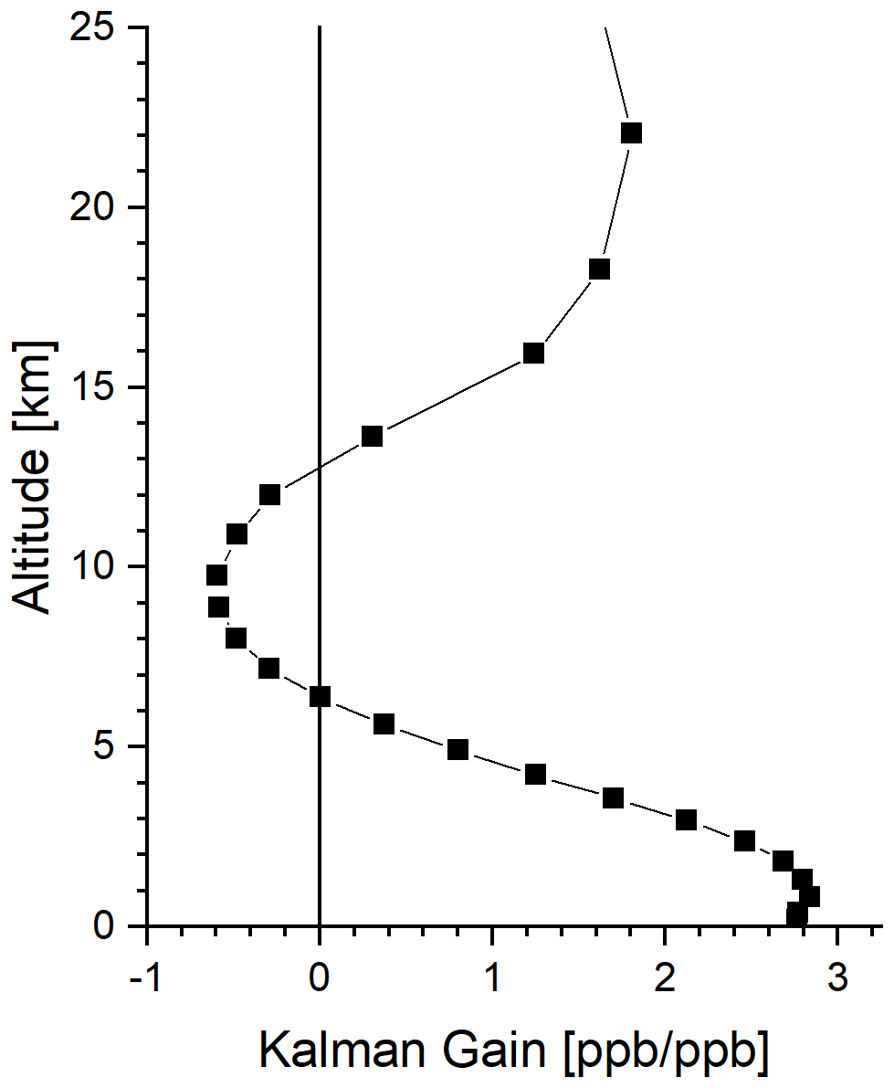
The column vector m is the Kalman gain operator, and it is given by
with the matrix and the scalar being the logarithmic-scale a posteriori covariance of the MUSICA IASI CH4 product and the noise error variance of the TROPOMI XCH4 product, respectively. The vector operator is the transpose of the TROPOMI column averaging kernel; i.e. .
Except for the logarithmic-scale transformation, Eqs. (1) and (2) are analogous to Eqs. (B9) and (B10). As demonstrated in Appendix B, this kind of Kalman filter application has a strong similarity to an optimal estimation retrieval that uses a combined IASI and TROPOMI measurement vector (synergetic use of level 1 data). The application of this Kalman filter is possible because the MUSICA IASI data are provided with full information on a priori states, constraints, error covariances, and averaging kernels (Schneider et al., 2022), and because the TROPOMI data are provided together with their a priori state, averaging kernel, and retrieval noise error (Lorente et al., 2021a).
The Kalman gain according to Eq. (2) describes how differences between the MUSICA IASI and TROPOMI XCH4 product are used to update the MUSICA IASI CH4 profile. An example for a Kalman gain operator is depicted in Fig. 1. It shows that a positive difference of +1 ppb of will lead to a combined CH4 profile product that has been modified with respect to the MUSICA IASI CH4 product by almost +3 ppb in the lowermost troposphere, by about −0.5 ppb at 10 km, and by about +1.5 ppb above 20 km.
3.2 Vertical resolution and representativeness
In this section, we compare the vertical resolution and representativeness of the individual retrieval products with those achieved when combining the two retrieval products. According to Eq. (1), the averaging kernels for the combined data product can be calculated as
Here, and are the logarithmic-scale averaging kernels of the MUSICA IASI CH4 product and of the combined product (the MUSICA IASI CH4 product after being updated with the information provided by the TROPOMI XCH4 product), respectively. These are the kernels for the profile products represented in the number of atmospheric levels (nal); i.e. they are matrices of dimension nal × nal. Logarithmic-scale averaging kernels are also called fractional or relative averaging kernels (e.g. Keppens et al., 2015).
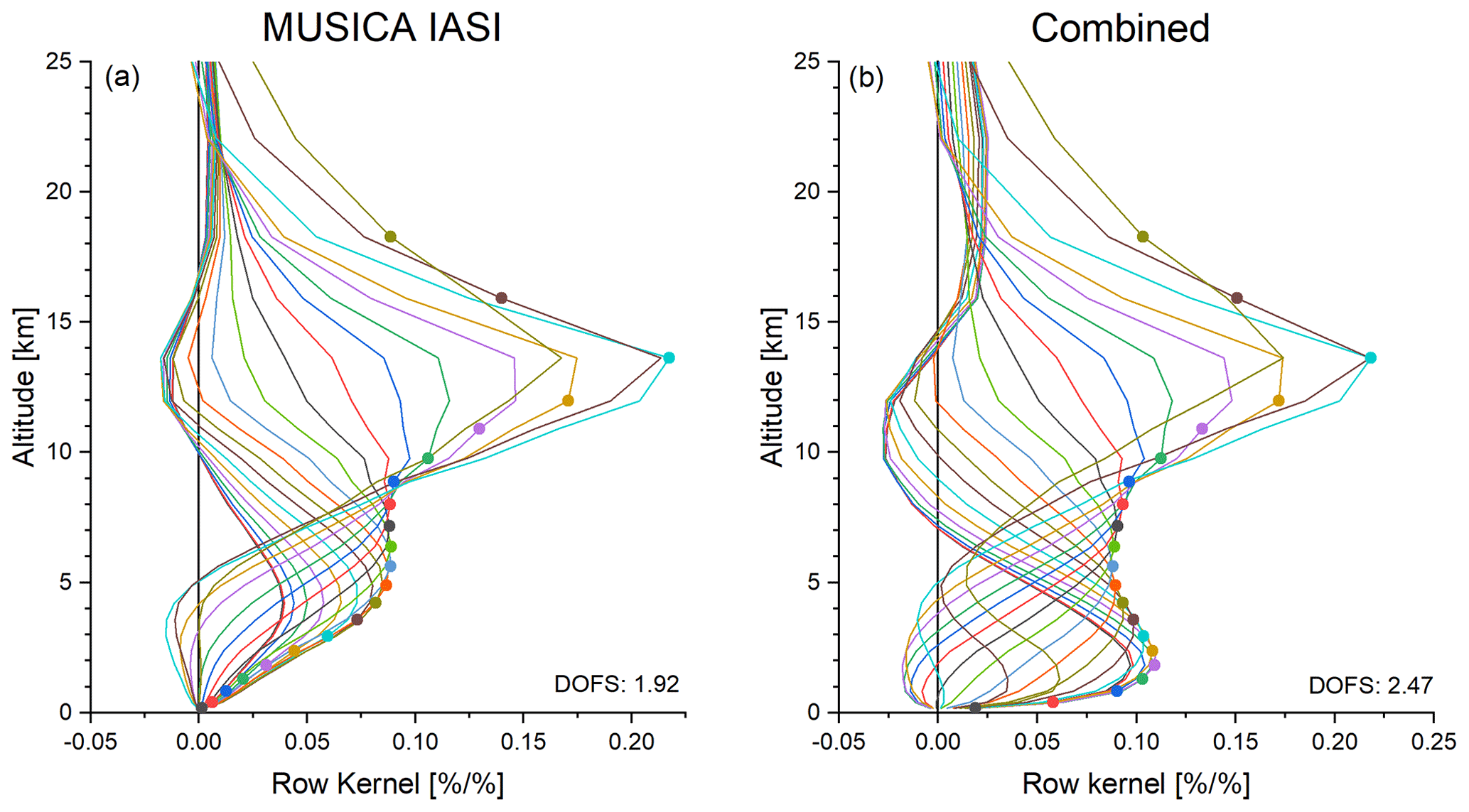
Figure 2 depicts the rows of typical averaging kernels for the MUSICA IASI product (Fig. 2a) and the combined data product (Fig. 2b). Adding the information provided by TROPOMI clearly improves the sensitivity in the lower troposphere: for the MUSICA IASI product, the lower tropospheric kernels generally peak at the upper limit of the lower troposphere (at about 5 km a.s.l.). For the combined product, these peak values are obtained at significantly lower altitudes (at about 2 km a.s.l.). In the UTLS, we see no significant difference between the kernels.
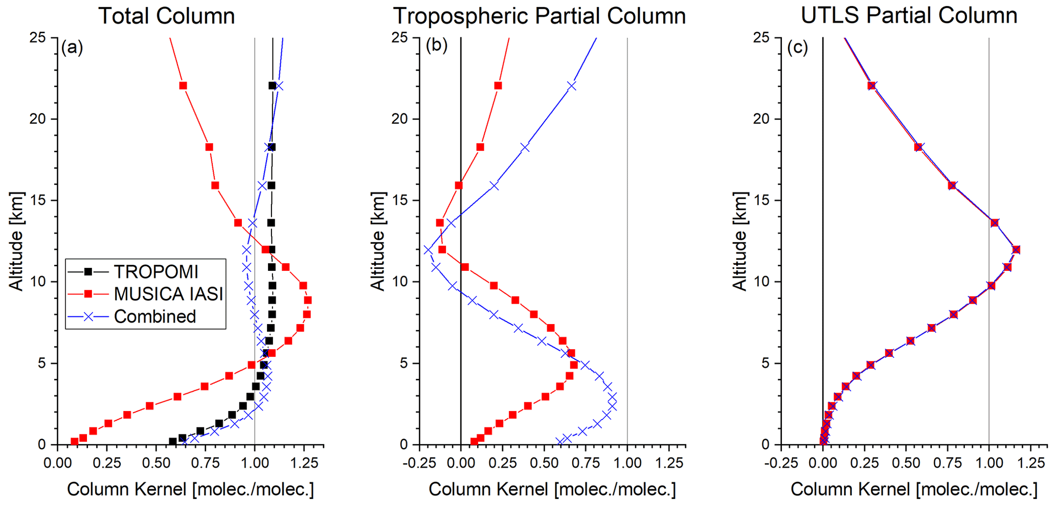
Figure 3Total-column and partial-column amount kernels corresponding to the TROPOMI, MUSICA IASI, and the combined product for the same late summer observation as used in Figs. 1 and 2: (a) total-column amount kernels; (b) lower tropospheric partial-column amount kernels, surface − 6 km a.s.l.; and (c) upper troposphere–lower stratosphere (UTLS) partial-column amount kernels, 6–20 km a.s.l.
In this work we focus on the total-column and the partial columns between the surface and 6 km a.s.l. (the tropospheric partial column) and between 6 and 20 km a.s.l. (the UTLS partial column). The total- and partial-column kernels are calculated from and by their transformation on a linear scale (see Appendix C) and the vertical resampling as explained in Appendix D. Figure 3 depicts the total- and partial-column kernels corresponding to the row kernels of Fig. 2.
Total-column amount kernels are available for all three products (see Fig. 3a): the TROPOMI, the MUSICA IASI, and the combined product. The TROPOMI kernel is close to unity for all altitudes, documenting the good sensitivity for CH4 at all altitudes. The combined total-column amount kernel is even closer to unity than the respective TROPOMI kernel, which means that the combined retrieval product does also reflect the actual atmospheric total-column amounts well. The MUSICA IASI kernel has relatively low values in the lower troposphere and above 15 km; only in the UTLS region are the kernel values between 0.75 and 1.25. This means that MUSICA IASI can actually not detect total-column amounts well because it lacks sensitivity in the lower troposphere. The altitude regions where the MUSICA IASI product has reduced sensitivities are the regions where TROPOMI's total-column information has the strongest impact on the combined product (see Fig. 1).
Partial-column amount kernels are only available for profile products, i.e. the MUSICA IASI and the combined product (MUSICA IASI updated with information from TROPOMI). Figure 3b shows tropospheric partial-column amount kernels. For the MUSICA IASI product, we observe values that are generally lower than 0.5. The highest values are achieved around 6 km a.s.l., i.e. at the upper boundary of the vertical layer we defined as the tropospheric partial column. The kernel of the combined product shows a good sensitivity, with peak values of almost 0.95 at 2.5 km a.s.l. and values above 0.75 for almost all altitudes between the surface and 6 km a.s.l.
UTLS partial-column amount kernels are depicted in Fig. 3c. The values are closest to unity for the altitudes that we attributed to the UTLS layer (altitudes between 6 and 20 km a.s.l.). There is almost no difference between the MUSICA IASI and the combined kernels, meaning that the information provided by TROPOMI has almost no effect on the UTLS partial column, which is because the MUSICA IASI product is already very sensitive to this altitude region.
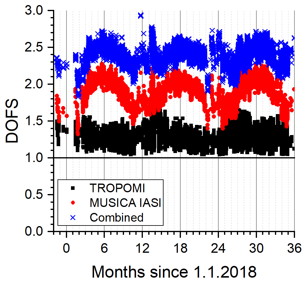
Figure 4Time series of the degree of freedom for signal (DOFS; example for central Europe). Black squares: TROPOMI (please note that only the total-column data are made available); red dots: MUSICA IASI; blue crosses: combined product.
The example kernels document that the combined product allows for detection of tropospheric CH4 largely independent from CH4 in the UTLS, which is not possible by the IASI product alone. Figure 4 shows a time series of the degree of freedom for signal (DOFS; it is calculated as the trace of the averaging kernels and is a measure for the profiling capability; Rodgers, 2000). It documents that the combination of TROPOMI with IASI improves the profiling capability of IASI rather consistently throughout all seasons. Here we also show the DOFS values of the TROPOMI retrieval, but please note that only the total-column data are made available; i.e. there is no profile information in the provided TROPOMI CH4 data product.
An optimal estimation retrieval updates the a priori knowledge with information provided by a measurement. The a posteriori uncertainty is the uncertainty achieved by optimally combing the a priori knowledge (captured by the inverse of the a priori covariance matrix, i.e. ) with the measurement. As shown in Appendix A, the a posteriori uncertainty covariance is the sum of the noise covariance and the representativeness error covariance (called “smoothing error” covariance in Rodgers, 2000).
According to Eq. (A7) the representativeness error matrix is calculated from the averaging kernel (A) and the a priori covariance (Sa) as
with I being the identity operator. By using the kernels and , we can calculate the representativeness error for the MUSICA IASI and the combined product, respectively. The resampling of on total and partial columns is done according to Eq. (D7). For the TROPOMI total-column-averaged mixing ratios we can calculate the representativeness error by . For more details, see Appendix D.
Figure 5 depicts the representativeness error relative to the retrieved values for the total column and the tropospheric and UTLS partial columns. Shown are time series for measurements over central Europe, which confirm the observations made in the context of the example kernels of Fig. 3: for the total column (Fig. 5a) the representativeness error on the TROPOMI and the combined products is rather small and can be neglected; i.e. both products can detect total-column signals. In contrast the MUSICA IASI representativeness error is much larger, and the respective data do not represent the total column well; i.e. they provide no independent observations of the total column. Concerning partial-column products (Fig. 5b and c), we can compare the MUSICA IASI and the combined product (the TROPOMI product has no information on the vertical distribution). The tropospheric MUSICA IASI partial column has a significant representativeness error (and a seasonal cycle with highest values of about 3 % in winter). In the combined product, this error is generally smaller than 1 % throughout all seasons. In the UTLS both the MUSICA IASI and combined products are strongly representative of the actual atmospheric methane concentration signals (representativeness error is generally between 0.5 % and 1 %). In summary, TROPOMI only provides total-column data. With IASI alone, we can detect signals in the UTLS well but not in the lower troposphere. The detection of signals in both altitude regions independently from the a priori information is only possible using the combined product.
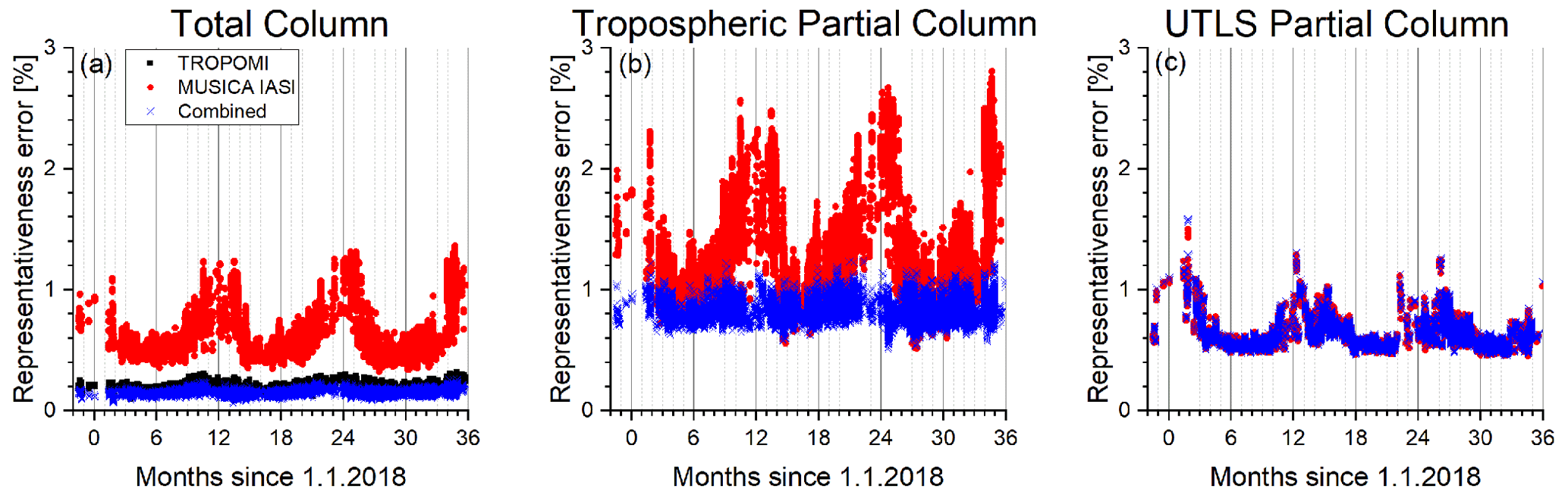
Figure 5Time series of the representativeness error (example for central Europe). Black squares: TROPOMI; red dots: MUSICA IASI; blue crosses: combined product. (a) Total column, (b) tropospheric partial column, and (c) UTLS partial column.
3.3 Retrieval noise error
After documenting the representativeness error in the previous subsection, here we investigate the retrieval noise error. We compare the retrieval noise errors of the individual retrieval products with those achieved when combining the two retrieval products. According to Eq. (1), we can calculate the retrieval noise covariance matrix for the combined data product by
Here is the retrieval noise covariance matrix of the MUSICA IASI retrieval. The error covariances resampled to the total and partial columns are then determined according to Appendix D. Figure 6 shows the retrieval noise errors (which are the square root values of the error variances) relative to the retrieved values for the total column and the tropospheric and UTLS partial columns.
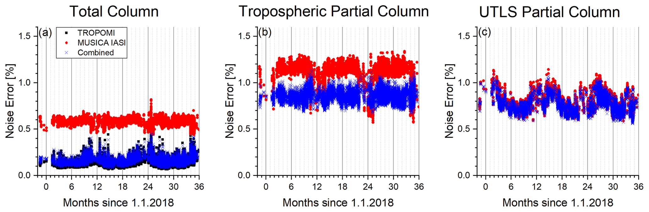
Figure 6Time series of estimated relative noise error for the retrieved products (example for central Europe). Colours are as in Fig. 5. (a) Total column, (b) tropospheric partial column, and (c) UTLS partial column.
The errors for the total columns (Fig. 6a) are generally below 0.2 % for the TROPOMI product. For the MUSICA IASI product, they are rather stable at about 0.6 %. Concerning the combined product, the retrieval noise error is very similar to the retrieval noise error of the TROPOMI data.
For the tropospheric partial columns (Fig. 6b), the error is in general above 1 % for the MUSICA IASI product and below 1 % for the combined product. For the UTLS partial columns (Fig. 6c), we observe an error of generally below 1 % and no significant difference between the MUSICA IASI and the combined data products. This suggests that the error in the combined product is dominated by the error in the MUSICA IASI data, which reveals the very limited impact of the TROPOMI data on the combined UTLS data product.
3.4 Dislocation error
As mentioned in Sect. 2.3, we allow for small dislocations between the TROPOMI and IASI observations of up to 6 h and 50 km. As derived in Appendix E, the dislocation error covariance matrix is calculated by
where is the dislocation kernel, and is the covariance matrix for the CH4 dislocation uncertainty, whose main characteristics are visualized in Figs. E1 and E2. The low entry of the dislocation kernel at low altitudes (for a typical example, see Fig. E4) reduces the impact of the spatial and temporal dislocation on the total and tropospheric partial columns of the combined product.
Over central Europe, we estimate an error in the combined product due to the dislocations between IASI and TROPOMI as shown in Fig. 7. For the total column, the error is below 0.1 %, and for the tropospheric and UTLS partial columns, it is generally below 0.8 %. If compared to the noise error (see Fig. 6), the dislocation error is of secondary importance. Details on the estimation of these dislocation errors and examples for other locations are given in Appendix E.
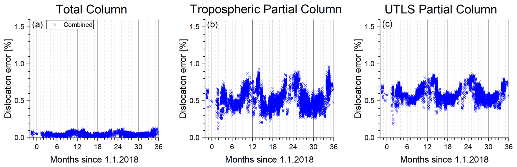
Figure 7Time series of estimated relative dislocation error for the combined product due to temporal and spatial dislocation of the TROPOMI and IASI satellite ground pixels (example for central Europe). (a) Total column, (b) tropospheric partial column, and (c) UTLS partial column.
In this section we empirically evaluate the quality of the TROPOMI, MUSICA IASI, and combined products by their inter-comparison to different reference data products. As reference for the total-column-averaged mixing ratio (XCH4), we use TCCON (Total Carbon Column Observing Network; Wunch et al., 2011a) ground-based remote-sensing data from 14 sites located in different climate zones. As reference for the total and the partial columns, we use in situ profiles measured by the AirCore system (Karion et al., 2010) at two geophysically different European locations. Furthermore, we use in situ data measured at two nearby central European Global Atmospheric Watch (GAW) mountain stations.
Figure 8 depicts the geographical location of the reference observations. Figure 8a shows that the considered TCCON stations are distributed around the globe (more detailed information on these sites is given in Table 1). Figure 8b gives details on the different European reference sites and the areas accepted for a valid collocation. For collocation with TCCON, the satellite ground pixels should fall within a circle around the stations with a radius of 100 km (red crosses and circles). For the comparison to the GAW data, the collocation circle has a radius of 150 km (grey circle) and is centred in the middle of the two GAW stations (Jungfraujoch in Switzerland and Schauinsland in south-western Germany, indicated by the grey dots). For the comparison with AirCore, we relax the radius of the collocation circle to 500 km in order to achieve a sufficient high number of coincidences between AirCore and satellite observations. The two AirCore sites (Trainou in France and Sodankylä in Finland) and the collocation circles are indicated by the blue stars and circles.
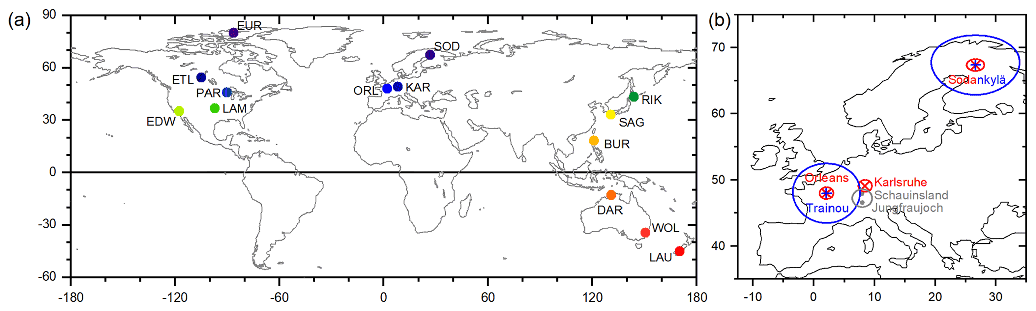
Figure 8Maps showing the location of the reference measurements used for the validation. (a) Global map with the 14 TCCON stations (more detailed information on these sites is given in Table 1). (b) Map indicating the areas accepted for valid horizontal collocations in the surroundings of the European reference stations: TCCON sites and the 100 km collocation radius (red crosses and circles), AirCore sites and the spatial collocation circles with 500 km radius (blue stars and circles), and GAW sites and the collocation circle with 150 km radius (grey dots and circle).
Appendix F reveals that the following validation results are in reasonable agreement with sensitivities and errors of the different satellite data products as shown in Sects. 3.2–3.4.
4.1 TCCON XCH4
We use TCCON ground-based remote-sensing data from 14 sites located in different climate zones representative of high, middle, and low latitudes. Details on the locations of these sites, the respective data amounts, and references are given in Table 1. We use the TROPOMI a priori setting for the comparison between the ground-based TCCON and the satellite-based remote-sensing products. For this purpose the TCCON product is adjusted to the TROPOMI a priori settings according to Eq. (B13), which ensures the usage of the same a priori data for all the remote-sensing products. As spatial collocation criteria, we require the TROPOMI and IASI ground pixels to be located within 100 km of the TCCON station (where we consider the viewing direction of the TCCON spectrometer by using as location, the TCCON's line of sight {latitude, longitude} at 5 km altitude). Differences in the satellite and TCCON ground pressures are taken into account by correcting the TCCON XCH4 values according to Appendix B of Sha et al. (2021). For collocation with respect to time, as TCCON reference we use the median XCH4 value calculated from all TCCON data measured within 2 h of the TROPOMI observation. Furthermore, we require stable conditions for atmospheric CH4. This is achieved by performing the comparisons only if there are at least three individual TCCON observations that fulfil the collocation criterion, if the timestamps of these observations have a 1σ standard deviation of 1 h, and if the 1σ standard deviation of the respective XCH4 data is smaller than 0.5 %.
Strong et al. (2019)Kivi et al. (2014)Kivi and Heikkinen (2016)Wunch et al. (2018)Hase et al. (2015)Warneke et al. (2019)Wennberg et al. (2017)Morino et al. (2018)Wennberg et al. (2016)Iraci et al. (2016)Kawakami et al. (2014)Velazco et al. (2017)Griffith et al. (2014a)Griffith et al. (2014b)Sherlock et al. (2014)Pollard et al. (2019)Table 1Locations of TCCON sites, amount of the satellite data compared to TCCON, and references. “Number” gives the total number of single satellite footprint collocations and “Days” the number of days with collocations.
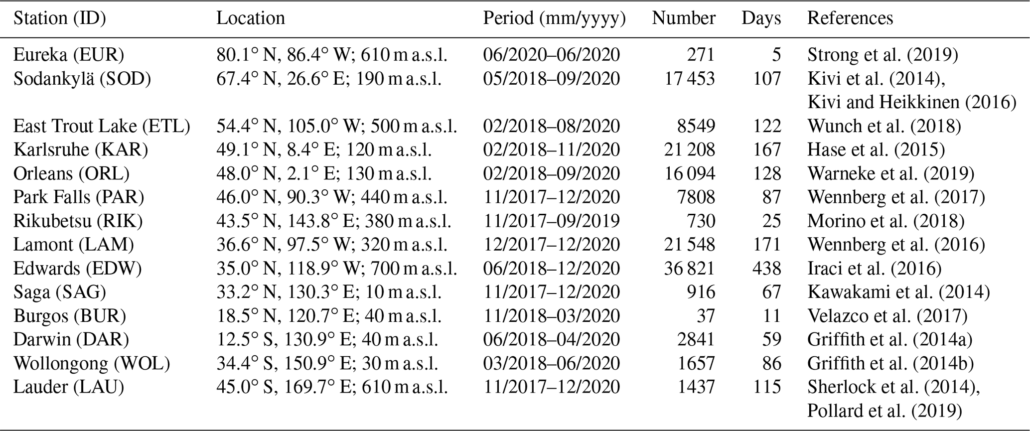
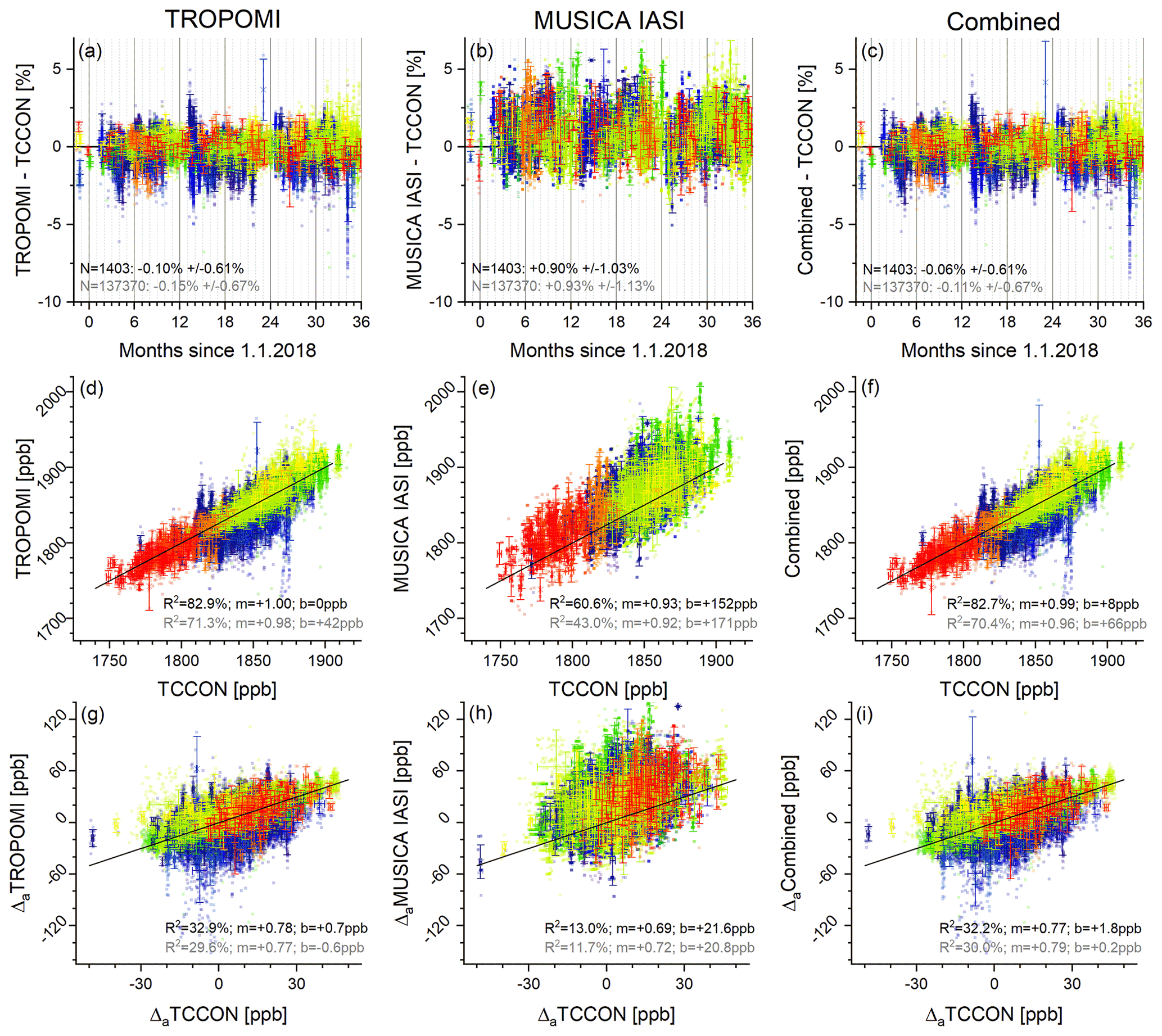
Figure 9Comparison of the different XCH4 satellite products with TCCON XCH4 data from 14 globally representative stations (the different colours correspond to the stations as shown in Fig. 8a). Data for all individual coincidences are plotted in the background as squares, and daily mean data are depicted as crosses with error bars representing the 1σ standard deviation (daily means are only calculated if there are at least three observations per day): (a–c) time series of the differences. (d–f) Correlations between TCCON and satellite data (the black line is the one-to-one diagonal). (g–i) Correlations between the a priori free TCCON data () and the a priori free satellite data (). The inserted text reports median and scatter (hIPR68.2; a–c) and the coefficients of determination, the slope, and the intercept of the robust linear regression model (R2, m, and b; d–i). Black and grey fonts represent the values for the daily mean data and for data from all individual collocations, respectively.
In Fig. 9 the TROPOMI, MUSICA IASI, and combined XCH4 products are compared to the TCCON XCH4 data. The crosses represent the daily mean data, and the filled symbols in the background show all data corresponding to all individual valid collocations (between all single pixel satellite observations and individual TCCON observations). Figure 9a–c show time series of the differences with respect to the TCCON references. The daily mean data have error bars, which is the 1σ standard deviation of the data used for calculating the daily mean.
Statistics in form of the median of the difference and the scatter around the median difference are given in each panel (for statistics using daily mean data in black fonts and for statistics using all individual valid collocations in grey fonts). Here we use the median in order to be less affected by outliers. For the same reason, as metric for the scatter we use the half inter-percentile range between the 15.9 and 84.1 percentiles (hIPR68.2, which is analogous to the 1σ standard deviation in case of a pure Gaussian distribution). Concerning TROPOMI (Fig. 9a), we observe a good agreement. For daily mean data as well as for the statistics based on all individual differences, the median difference is within 0.1 %, and the scatter lies below 0.7 %.
A similar good agreement and low values for median difference and scatter are also achieved for the combined product (Fig. 9c). For the MUSICA IASI product (Fig. 9b), we have reduced sensitivity in the lower troposphere (see Figs. 3 and 5). Because of uncertainties in the a priori assumptions, the agreement with the TCCON XCH4 data is weaker (uncertainties in the a priori assumption are less well detected; see Fig. F2). We observe no significant systematic negative or positive difference for the satellite versus TCCON comparisons; i.e. the satellite data sets seem to be in good absolute agreement with TCCON. In general the observed scatter values are within the range that can be expected from the data uncertainties and the data comparability (for more details, see Appendix F).
Figure 9d–f depict the correlation plots. In order to reduce the effect of outliers, we apply a robust linear regression model (the iteratively reweighted least-squares algorithm with Tukey's bisquare weight function and the respective tuning parameter set to the commonly used value of 4.685). For daily mean data the obtained coefficients of determination (R2) are larger than 80 % for the TROPOMI and the combined product. The slope of the obtained linear regression line is very close to unity. When considering all individual coincidences, the R2 values are about 70 %. The error bars on the daily mean data are the 1σ standard deviations of the data used for calculating the daily mean. For the MUSICA IASI product, we observe a similar good correlation as for the TROPOMI and the combined products. However, concerning the MUSICA IASI data, part of the common signal might be due to the a priori data on which the MUSICA IASI total-column product is not independent (the MUSICA IASI data have a reduced sensitivity, i.e. an increased representativeness error; see Fig. 5a).
Figure 9g–i reveal the information gained by the satellite data with respect to the a priori data. The correlation is depicted between the collocated a priori free TCCON data () and the a priori free satellite data (). The same data as in Fig. 9d–f are shown but with the a priori knowledge removed. We find that the TROPOMI and the combined data product add a significant amount of information to the a priori knowledge (R2 values for the respective linear correlations of above 32 %). This information gain is much smaller in the case of the MUSICA IASI data, which confirms that the good correlation as observed in Fig. 9e is to a large extent due to the good quality of the a priori data.
4.2 AirCore in situ CH4 profiles
We use the AirCore balloon-borne in situ measurements (Karion et al., 2010) as the reference for CH4 total columns as well as for the CH4 vertical distribution. The AirCore system samples the vertical distribution of CH4 with a much better vertical resolution than the satellite remote-sensing systems. For this reason, we can generate an AirCore profile () that has the same vertical sensitivity and resolution characteristics as the remote-sensing data. According to Eqs. (A2) and (A4), for the MUSICA IASI and the combined retrieval data we can write
Here Al and are the logarithmic-scale averaging kernels and the logarithmic-scale a priori state of the satellite retrieval, respectively, and is the measured logarithmic-scale AirCore profile regridded to the atmospheric model grid used for the satellite retrievals. The resampling of these data on total and partial columns is done with the linear-scale data according to Eq. (D5). For the TROPOMI total-column-averaged mixing ratios, we calculate the adjusted AirCore total-column-averaged mixing ratio (a scalar) by . For more details, see Appendix D.
As spatial collocation criteria, we require that the ground pixels of the TROPOMI and IASI measurement fall within a circle with a radius of 500 km around the mean horizontal location of the AirCore system when sampling between the 450 and 550 hPa pressure levels. The temporal collocation requirements for both satellite observations is 6 h. AirCore data are typically not available close to the ground and above the burst altitude of the balloon (approximately 25 hPa). At low altitudes we extend the profile with the concentrations closest to the ground. At high altitudes we extend the profile with the TM5 model data, with a smooth transition between the measured values and the modelled data.
Table 2 gives an overview of the satellite data amount compared to the AirCore profiles measured at Trainou (France; 48.0∘ N, 2.1∘ E) and Sodankylä (Finland; 67.4∘ N, 26.6∘ E). In total we have 36 individual AirCore profiles measured on 31 different days for which collocated satellite observations exist. The total number of collocated single pixel satellite observations is 34 784. We estimate that the AirCore data can serve as reliable references for the validation of the total column as well as for the validation of the tropospheric and UTLS partial columns (see Appendix F).
Table 2Locations of AirCore sites and amount of satellite data compared to AirCore. “Number” gives the total number of single satellite footprint collocations, “Days” the number of days with collocations, and “AC number” the number of collocated AirCore profiles.
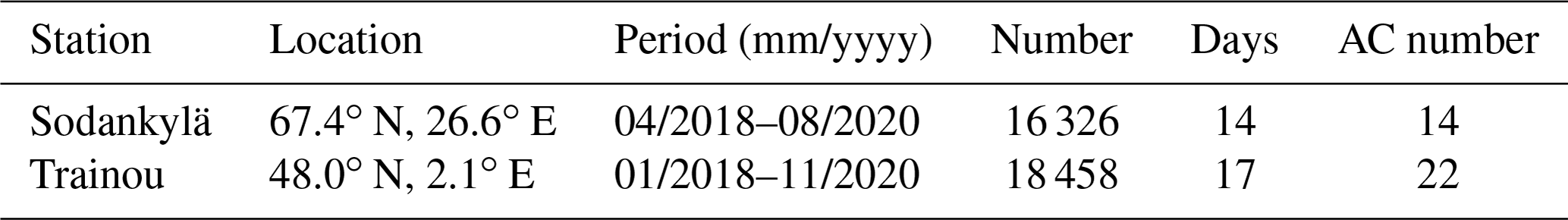
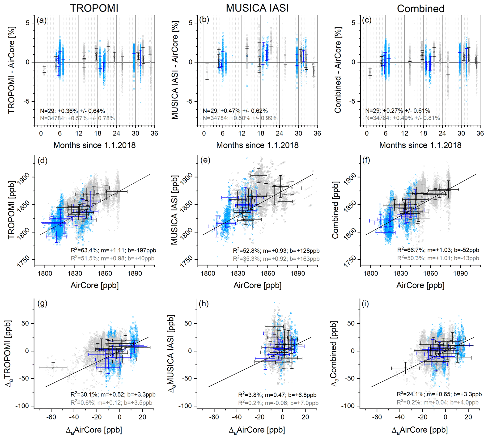
Figure 10Comparison of the different satellite XCH4 products with adjusted AirCore XCH4 measured at Trainou (black) and Sodankylä (blue). Data for all individual coincidences are shown in the background as pale crosses, and daily averages are depicted as crosses with error bars (daily means are only calculated if there are at least three observations per day, which is the case on 29 d of the total 31 d with AirCore observations). (a–c) Time series of the differences (error bars represent the daily 1σ standard deviation of the difference). (d–f) Correlation between AirCore and satellite data (the black line is the one-to-one diagonal, and the x-axis error bars represent the mean uncertainty estimated for the AirCore data – according to Eq. (F3) – and y-axis error bars the daily 1σ standard deviation of the satellite data, respectively). (g–i) Correlation between the a priori free AirCore and satellite data (error bars as in d–f). The inserted text reports median and scatter (hIPR68.2; a–c) and the coefficients of determination, the slope, and the intercept of the robust linear regression model (R2, m, and b; d–i). Black and grey fonts represent the values for the daily mean data and for data from all individual collocations, respectively.
The comparison between the satellite and the AirCore XCH4 data is shown in Fig. 10. The differences of collocated measurements are shown in Figs. 10a–c. The agreement between the different satellite products and AirCore is good: the scatter around the median difference is low and similar to the comparison with TCCON. Furthermore, we observe no significant bias in any of the satellite data, which demonstrates the good consistency between the RemoTeC TROPOMI and MUSICA IASI XCH4 data.
Figure 10d–f depict the correlation between the satellite and the adjusted AirCore data. Here we apply the same iteratively reweighted least-squares as in Sect. 4.1. The obtained R2 values are high (for all products above 60 % for daily mean data) although a bit lower than the R2 value achieved for the correlation with TCCON data; however, we have to consider that the amplitude in the analysed total-column signals is much smaller in the AirCore data set (data from two northern hemispheric sites only) if compared to the TCCON data set (data from 14 globally distributed sites). As for the comparison to TCCON, we examine the correlation between the a priori free reference data () and the a priori free satellite data (). These correlations are visualized in Fig. 10g–i. We find reasonable correlation for the daily mean TROPOMI and combined data products but no significant correlation for the daily mean IASI product. This indicates that the correlation as observed between the IASI and the adjusted AirCore data in Fig. 10e is mainly due to the a priori data; i.e. IASI adds almost no information with respect to XCH4 to what is already known by the a priori model. These findings are in line with the vertical resolution and representativeness analyses of Sect. 3.2.
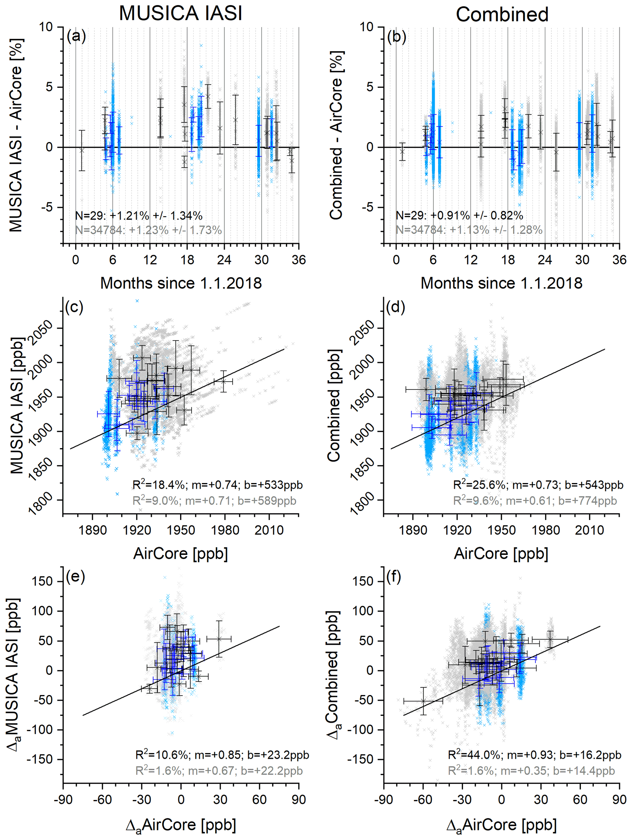
Figure 11Same as Fig. 10 but for the comparisons of tropospheric partial-column-averaged CH4 AirCore and satellite products (IASI and combined).
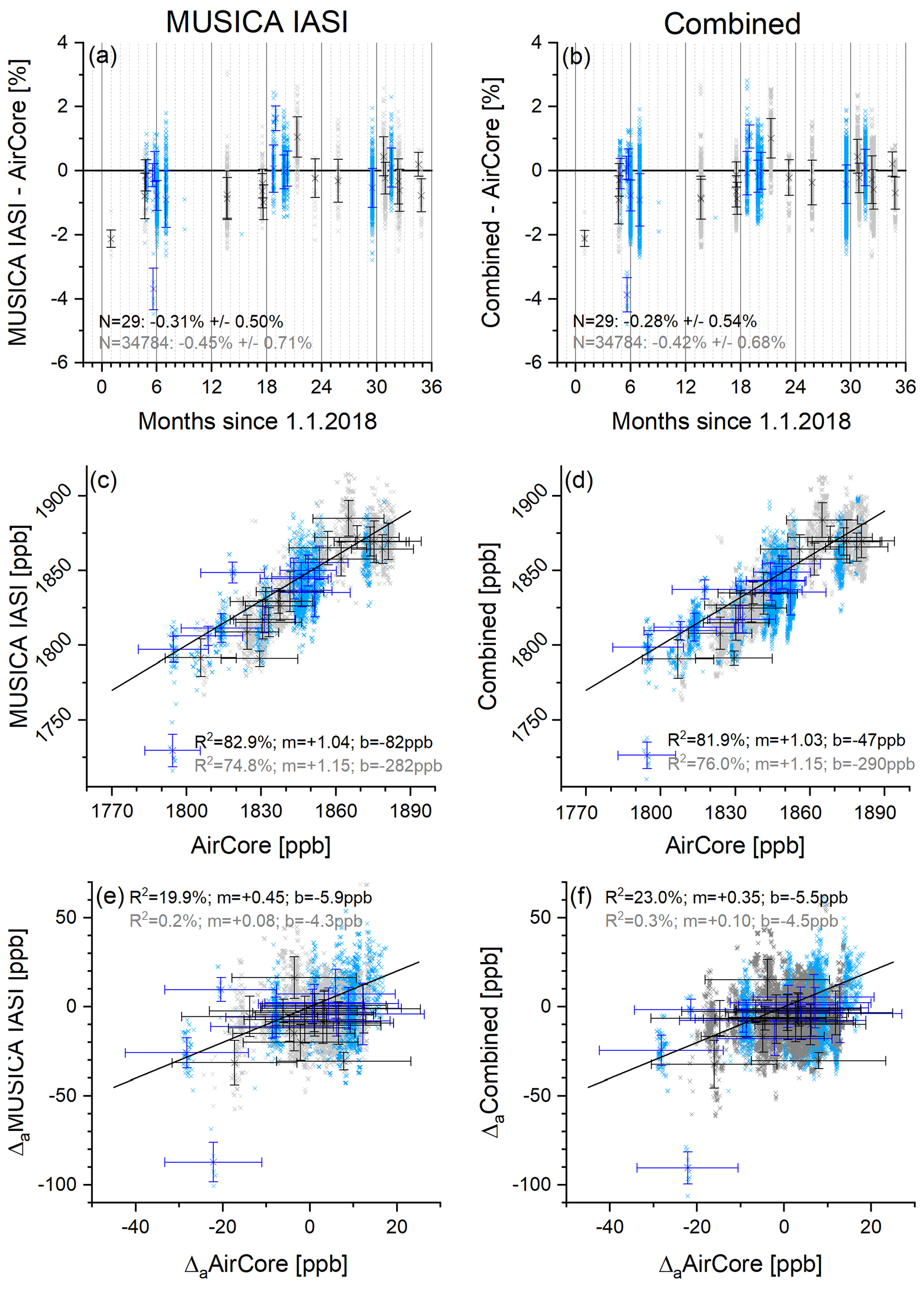
Figure 11 presents the comparison between the AirCore and satellite tropospheric partial-column CH4 data. The differences between the satellite and the AirCore data are depicted in Fig. 11a and b. If compared to the total-column data, the agreement worsens a bit (increased median difference and scatter). Nevertheless, the agreement is still good and close to what can be expected from the uncertainty and the comparability of the different data (see Appendix F). Concerning the daily mean data, the combined product has a median difference and hIPR68.2 scatter of below about 0.9 %. These values increase to about 1.25 % for the IASI product. These results might indicate a weak systematic bias in the MUSICA IASI lower tropospheric partial columns.
Figure 11c and d show the correlation plots. In particular for the combined product we observe a reasonable correlation (R2 of about 26 % for daily mean data obtained using the robust linear regression model). For the IASI product the correlation strength is reduced (R2 of about 18 % for daily mean data). Furthermore, we have to consider that the IASI product has a rather limited tropospheric sensitivity (see Sect. 3.2), which means that a large part of the observed correlation is due to the a priori data: according to Eq. (7), for low entries in Al the variability in the satellite data as well as in the adjusted AirCore data is determined by the variability in the a priori (). This is confirmed by Fig. 11e and f, which show the correlations after removing the a priori data. We still observe a good correlation for the combined product (R2 of about 44 % and regression line slope of 0.93 for daily mean data) but only a weak correlation for the IASI daily mean data (R2 of about 11 %). This clearly documents the importance of combining IASI and TROPOMI in order to be sensitive to and reliably detect tropospheric CH4 variations.
Concerning the UTLS partial column, we find a very good agreement between the adjusted AirCore data and the IASI and combined satellite data products (see Fig. 12a, b): the median difference calculated from the daily mean data is about −0.3 %, and the scatter values are within about 0.5 %. We find no indication of a bias in the satellite data product. The scatter observed between the AirCore and satellite data is even better than what we estimate from the data uncertainty and the data comparability analysis (see Appendix F). Figure 12c and d show that in the UTLS the AirCore and satellite data are strongly correlated (for daily mean data and when using the robust linear regression model, we get R2 values of up to about 82 % and regression line slopes of very close to unity). In this altitude region the MUSICA IASI and the combined products have a very good sensitivity (see Sect. 3.2). This means that the entries in Al of Eq. (7) are large, and any deviation between the a priori and the actual CH4 concentrations in the UTLS are captured well by the adjusted AirCore and satellite data products. Nevertheless, the correlation strength observed for the a priori free data (Fig. 12e, f) is relatively weak (R2 values of 20 %–23 % for daily mean data). This indicates that the a priori model does generally capture well the actual variation of the CH4 concentration in the UTLS above France and northern Scandinavia.
4.3 GAW surface in situ CH4 measurements
At many globally distributed sites, atmospheric trace gas in situ measurements are made continuously within the Global Atmospheric Watch (GAW; https://community.wmo.int/activity-areas/gaw, last access: 5 July 2022) programme. Appendix A of Sepúlveda et al. (2014) presents a method for filtering common signals in night-time CH4 data of the two nearby mountain GAW stations Jungfraujoch (46.5∘ N, 8.0∘ E; 3580 m a.s.l.) and Schauinsland (47.9∘ N, 7.9∘ E; 1205 m a.s.l.). Data were retained as common signals when deviations of observations (after correction for vertical gradient, i.e. application of an offset, and a temporal shift in the annual cycles) at both sites were below a certain threshold. Sepúlveda et al. (2014) showed that the common signals are strongly representative of a broader layer in the lower free troposphere. Here we follow this approach and use the mean of the Jungfraujoch and Schauinsland CH4 mixing ratio – whenever identified as a common signal – as a validation reference for the remote-sensing data in south-western Germany and northern Switzerland (indicated by the grey circle in Fig. 8b). We assume that the signals obtained from this GAW data filtering are strongly representative of the tropospheric partial-column-averaged mixing ratios (surface–6 km a.s.l.) and compare these data directly to different satellite products as a fully independent data set: we do not adjust the data to a common a priori data usage as in Sect. 4.1 because the in situ data represent absolute measurements and do not depend on any a priori information. Furthermore, we do not adjust sensitivities as in Sect. 4.2 (see Eq. 7), which means that here we also validate the sensitivities of the products.
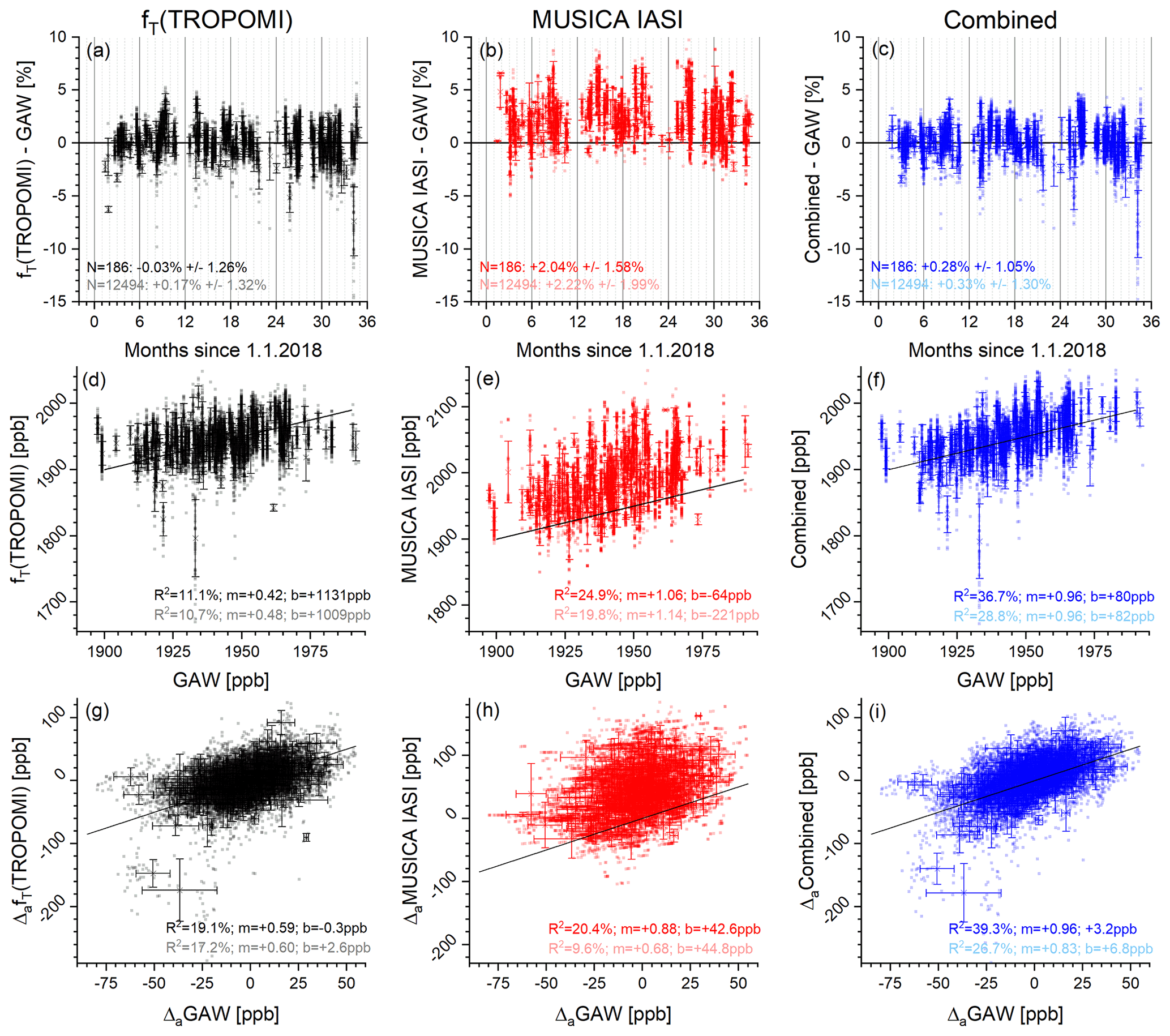
Figure 13Comparison of GAW measurements made at Jungfraujoch and Schauinsland with the TROPOMI tropospheric CH4 proxy product according to Eq. (8) and the IASI and the combined tropospheric CH4 products. Data for all individual coincidences are shown in the background as squares, and daily averages are depicted as crosses with error bars representing the daily 1σ standard deviations (daily means are only calculated if there are at least three observations per day). (a–c) Time series of differences. (d–f) Correlation between GAW and satellite data (the black line is the one-to-one diagonal). (g–i) Correlations between the difference of GAW and a priori data () and the a priori free satellite data (). The inserted text reports median and scatter (hIPR68.2; a–c) and the coefficients of determination, the slope, and the intercept of the robust linear regression model (R2, m, and b; d–i). Dark and pale coloured fonts represent the values for the daily mean data and for data from all individual collocations, respectively.
In order to be able to compare TROPOMI data to the GAW data, we calculate a proxy (fT(TROPOMI)) from the TROPOMI XCH4 data that represents the tropospheric column-averaged mixing ratios:
In Eq. (8) Xair and troXair are the dry-air total and tropospheric partial columns, respectively, and troXCH4(a priori) is the tropospheric column-averaged CH4 a priori data. In the case that the CH4 a priori data in the UTLS is of very good quality, this proxy is strongly representative of the tropospheric CH4 variations.
Figure 13 shows the comparison with the different satellite products. For the tropospheric proxy product calculated from the XCH4 product of TROPOMI, we observe no systematic difference and a scatter of the daily mean differences of within 1.3 % (Fig. 13a). However, the correlation is rather weak (from the robust linear regression model we get R2 values of about 10 % and regression line slope m of below 0.5; see Fig. 13d), which might suggest that this proxy is affected by signals in the UTLS, where CH4 values are dominated by shifts of the tropopause height.
For the MUSICA IASI tropospheric partial-column-averaged mixing ratio product (Fig. 13b, e) we observe a smaller median difference than for the comparison with the TROPOMI tropospheric proxy CH4 data but at the same time an increased scatter. The R2 values are larger than for the correlation of TROPOMI proxy data; however, we have to be careful because in the lower troposphere, the MUSICA IASI CH4 data have a limited sensitivity (see Fig. 5b). This means that the respective data are significantly affected by the a priori assumptions, and the observed correlation might actually be due to a correlation with the tropospheric a priori data. This is confirmed by Fig. 13h, which shows the correlation after removing the a priori data. Then the correlation strength is weaker if compared to the data that include the a priori information (R2 decreases from about 25 % to 20 % and from about 20 % to 10 % for correlations with daily mean and all individual data, respectively).
The combined product has a good sensitivity in the troposphere (see Fig. 5b); i.e. the respective partial-column-averaged mixing ratio product is practically independent from the a priori assumptions. We find a good agreement and correlation between the GAW data and the combined products as illustrated in Fig. 13c and f: for instance, for daily mean data, the difference and scatter is +0.28 % ±1.05 %, the R2 value is about 37 %, and the regression line slope is very close to 1.0. This demonstrates that the combined product can reliably capture actual tropospheric CH4 variations independently from the UTLS CH4 variations and from the a priori assumption. The latter is confirmed by Fig. 13i, which shows the correlation after removing the tropospheric a priori information. We observe that the good correlation remains, even after removing the a priori information (for daily mean data the R2 value is about 39 % and the regression line slope close to 1.0). A similar good correlation is not achieved by the TROPOMI tropospheric proxy and the IASI product.
5.1 Discussion on global data consistency
The TCCON and AirCore comparisons of Sects. 4.1 and 4.2 suggest that the combined total-column and UTLS partial-column products have no significant bias with respect to reference data. However, there might be a weak bias in the troposphere (see discussions in the context of Fig. 11). In general we have to consider that the study on biases in the profile data is limited to the two sites where AirCore references are available: Sodankylä in northern Scandinavia and Trainou in France. In this section, we argue that it is reasonable to assume similar insignificant or low biases also for other locations.
According to Eq. (A2) a varying error in the a priori state together with a poor sensitivity (i.e. an averaging kernel being very different from an identity matrix) can cause a varying bias. If the error in the a priori state is latitudinally dependent, the bias will also be latitudinally dependent. Similarly, a systematic error source (like an error in a spectroscopic parameter) can have a variable impact on the remote-sensing product, if the sensitivity is variable. If the sensitivity has a dependency on latitude, a systematic error source can thus also cause a latitudinally dependent bias. In this context, variabilities (e.g. latitudinal dependencies) of biases are likely for a low or variable sensitivity. In contrast, inconsistencies in the bias are unlikely in the case of a high and constant sensitivity (as observed in Fig. 5 for the total column and tropospheric and UTLS partial columns of the combined data product).
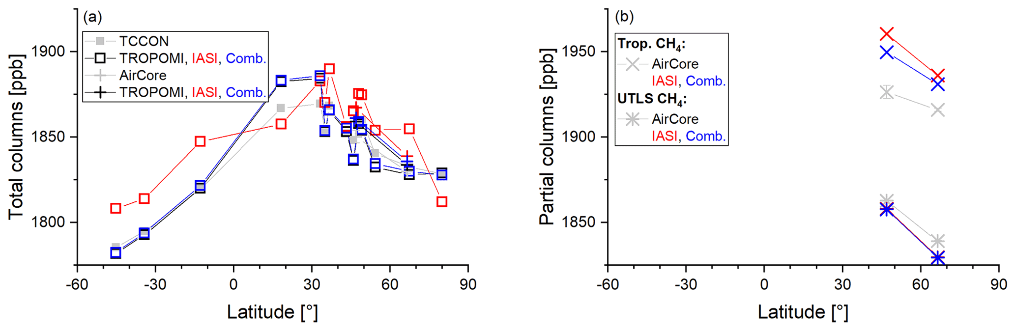
Figure 14Latitudinal dependency of the overall mean values obtained at the 14 TCCON and two AirCore observation sites. Grey colour represents the TCCON and AirCore reference data and black, red, and blue colours the TROPOMI, MUSICA IASI, and combined satellite data, respectively: (a) for total columns (XCH4) and (b) for tropospheric and UTLS partial columns. The error bars on the AirCore data describe the variability range due to the AirCore data treatment – according to Eq. (7) – with the different averaging kernels of the TROPOMI, MUSICA IASI, and combined data product.
Figure 14 depicts the overall mean total- and partial-column values obtained at the 14 TCCON and two AirCore observation sites. For total-column data (Fig. 14a), we achieve a good latitudinal coverage by the TCCON observation sites and can investigate possible latitudinal inconsistencies in the satellite data products. We find that the TROPOMI product and the combined satellite data product capture a latitudinal dependency that is similar to the dependency as seen in the TCCON data.
Figures 3a and 5a reveal that for the TROPOMI and the combined XCH4 products, the sensitivities are very high and stable, in contrast to the MUSICA IASI data product, which has a relatively weak and seasonally (and supposed latitudinally) varying sensitivity. This explains that in Fig. 14a the latitudinal dependency of the MUSICA IASI XCH4 data is different from the TCCON data. Table 3 resumes the statistics done with the overall mean XCH4 values obtained for the 14 TCCON observation sites. For the TROPOMI and the combined data product, the 1σ standard deviation calculated from the mean difference of the 14 stations is about 0.4 %. A standard linear least-squares fit results in R2 values of almost 100 % and regression line slope values of close to unity, which confirms the very good latitudinal data consistency of the TROPOMI and combined data products. The MUSICA IASI XCH4 product shows poorer performance with regard to the values of standard deviation and R2, which is in line with its weak and varying sensitivity.
Table 3Statistics based on the comparisons between satellite and TCCON data of the overall mean XCH4 values obtained for the 14 TCCON sites of Table 1.

A similar study of the latitudinal consistency of the partial-column data products is compromised by the lack of profile references for low latitudes and southern hemispheric sites (Fig. 14b). Nevertheless, because the combined product has a rather high and constant sensitivity for the tropospheric as well as the UTLS partial column (see Figs. 3 and 5), we expect – as for XCH4 – a good latitudinal consistency, i.e. a bias at low and/or southern latitudes that is similarly insignificant or as low as the biases observed at two AirCore stations in the middle and high northern latitudes.
5.2 Example of global maps
The proposed synergetic use method needs no extra retrievals and is thus computationally very efficient. This makes it ideal for combining the large TROPOMI and IASI data sets on global scale. Figure 15 shows monthly mean global maps ( resolution) of TROPOMI XCH4 data and the tropospheric and UTLS partial-column CH4 data of the combined product. The maps are generated from about 1.62 million and 3.77 million individual data points in January and July 2020, respectively. These are the data that remain after requiring collocation of the quality filtered IASI and TROPOMI data according to Sect. 2. TROPOMI alone only reports the XCH4 data (Fig. 15a, b). We observe low XCH4 values at high latitudes. The lowest values are encountered in the summertime Southern Hemisphere. The highest XCH4 values are present between northern low and middle latitudes. Here Fig. 15a and b show the TROPOMI data (the XCH4 data of the combined product are very similar). The combined product offers the most reliable tropospheric partial columns. Respective maps are shown in Fig. 15c and d. We observe partial-column-averaged CH4 mixing ratios that are almost monotonically increasing from south to north. In northern hemispheric winter (January 2020), this gradient is significantly stronger than in northern hemispheric summer (July 2020). The latitudinal patterns of tropospheric CH4 are significantly different from the respective patterns of XCH4, which might indicate to an extra potential of this tropospheric CH4 data when investigating the CH4 sources and sinks. Figure 15e and f show the respective maps of the UTLS partial columns (here we depict the combined data product; the respective MUSICA IASI data are very similar). We observe the highest partial-column-averaged mixing ratios at low latitudes (in January 2020 around the Equator and in July 2020 in the northern subtropics). The mixing ratios are lowest in high latitudes. This latitudinal pattern is in line with the tropopause height, which increases from high to low latitudes.
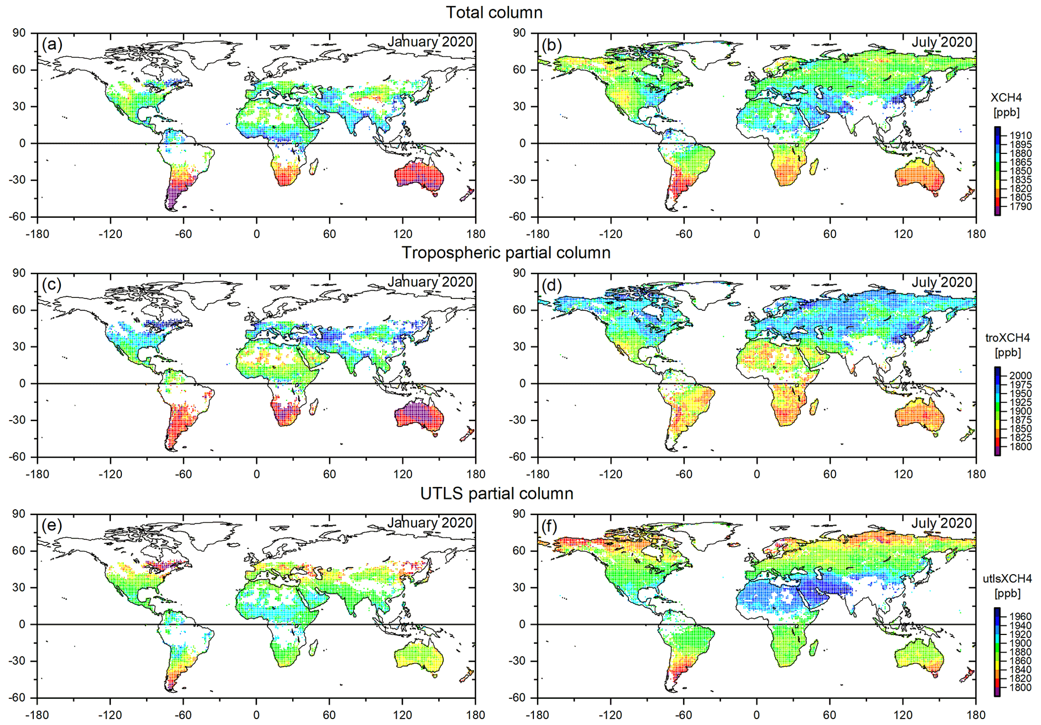
Figure 15Global maps with (longitude × latitude) resolution of monthly mean data for January and July 2020. (a, b) XCH4 as observed by TROPOMI. (c, d) Tropospheric partial columns of CH4 as obtained by the combined product. (e, f) UTLS partial columns of CH4 as obtained by the combined product.
We present a method for a synergetic combination of the IASI vertical profile and TROPOMI total-column level 2 retrieval products. It is computationally very efficient because it is based on simple linear algebra calculations that work with the output already available from individual IASI and TROPOMI retrievals. Nevertheless, theoretically it approximates closely to a computationally expensive multispectral retrieval that uses the TROPOMI and IASI level 1 data (see Appendix B). We apply the method to CH4 level 2 products. By providing a compilation with all important equations, we support its application to other data products.
We theoretically examine the sensitivity, vertical resolution, and errors of the individual TROPOMI and IASI products and of the combined product. The TROPOMI product consists of reliable total-column CH4 data but does not offer information on the vertical distribution. The IASI product offers some information on the vertical distribution and has the best sensitivity in the UTLS region but lacks sensitivity in the lower troposphere and in consequence to the total column. We show that the combined product combines both strengths: it is a reliable reference for the total column and also for the UTLS partial column. In addition, we found as a clear synergetic effect that the combined product is theoretically able to distinguish variations of CH4 that take place in the troposphere from variations at higher altitudes (it is a reliable reference for the tropospheric partial columns). We empirically demonstrate the functionality of the synergetic use method by comparing the different satellite CH4 products to reference data of TCCON, AirCore and GAW.
The TCCON data offer good references for XCH4. In this study we use data from 14 stations covering different climate regions in the Northern and Southern Hemisphere. For the TROPOMI and the combined data products, which are highly sensitive for XCH4, we get an agreement with the TCCON data within about 0.7 % (the agreement is slightly poorer with the IASI satellite product due to its reduced sensitivity).
AirCore offers XCH4 references as well as references for the vertical distribution of CH4. For this study 36 individual AirCore profiles measured at two sites in the northern hemispheric high and middle latitudes are available. Concerning XCH4, the comparisons to AirCore data confirm the results obtained by the comparison to TCCON data and in addition demonstrate a very good consistency between the TROPOMI and the IASI product. Concerning CH4 in the UTLS – where the MUSICA IASI and the combined data product are highly sensitive – we find that both products agree well with the respective AirCore references (agreement within 0.7 %).
The validation study with the TCCON and AirCore references shows that the total column and the UTLS partial column of the combined product has almost the same good quality as the respective products of TROPOMI and MUSICA IASI. This allows two conclusions: firstly, the assumption of the moderate non-linearity – required for a reliable functionality of the level 2 product combination according to Eq. (1) – is valid, and secondly, the combined product's tropospheric data are also of good quality (good total column and UTLS data quality is an indirect proof of a good tropospheric data quality).
The good quality of the combined product in the troposphere is in addition directly proven by the comparison to tropospheric reference data. We find an agreement of the daily mean tropospheric AirCore and combined product data within 1 %. This validation result is confirmed by the statistically very robust comparison with CH4 data observed continuously at two nearby GAW stations (the collocated GAW reference data cover all seasons for more than 3 years and represent more than 186 different days). The GAW and the combined product's data capture very similar tropospheric CH4 short-term variabilities and seasonal cycles. Similar good agreements are not achieved by comparisons to the individual MUSICA IASI or TROPOMI data products; i.e. we empirically and directly prove the synergetic effect of the level 2 product combination.
The proposed method takes benefit from the outputs generated by the dedicated individual TROPOMI and IASI retrievals; it needs no extra retrievals and is thus computationally very efficient. This is ideal for an operational combination of IASI and TROPOMI products in an efficient and sustained manner. This has a particular attraction because IASI and TROPOMI successor instruments will be jointly aboard the upcoming Metop-SG (Meteorological operational – Second Generation) satellites (guaranteeing observations from the 2020s to the 2040s). IASI and TROPOMI successor instruments will have globally distributed and perfectly collocated observations (over land) in the order of several hundred thousands per day, for which a combined product can be generated in a computationally very efficient way.
In this appendix, we give a brief overview of the theory of optimal estimation remote-sensing methods and follow the notation as recommended by the TUNER activity (von Clarmann et al., 2020), which is closely in line with the notation used by Rodgers (2000). The overview focuses on the equations that are important for our work, i.e. the a posteriori combination of two independently retrieved optimal estimation remote-sensing products. For a more detailed and general insight into the theory of optimal estimation remote-sensing methods, we refer to Rodgers (2000).
Atmospheric remote-sensing instruments measure radiance spectra (written as state vector y), which can be simulated by models (F) well whenever the actual atmospheric state (the vector x) is known. Using the a priori atmospheric state vector xa we can linearize and write
Here, K is the Jacobian matrix, i.e. derivatives that capture how the measurement vector (the measured radiances) will change for changes of the atmospheric state (the atmospheric state vector x). A remote-sensing retrieval inverts Eq. (A1) and provides an estimation of the difference between the atmospheric state and the a priori atmospheric state. For a moderately non-linear problem (according to Chapter 5 of Rodgers, 2000), the retrieved optimal estimation product () can be written as
G is the gain matrix and realizes the inversion from the measurement domain (radiances) to the domain of the atmospheric states. It consists of derivatives that capture how the retrieved atmospheric state vector will change for changes in the measurement vector:
with Sy,n and being the retrieval's noise covariance and the constraint matrices (in a strict optimal estimation sense, the constraint matrix is the inverse of the a priori covariance matrix Sa), respectively. The equivalence of both lines in Eq. (A3) is demonstrated in Chapter 4.1 of Rodgers (2000), where the first line is called the n form and the second line the m form.
The averaging kernel,
is an important component of a remote-sensing retrieval because according to Eq. (A2), it reveals how changes of the actual atmospheric state vector x affect the retrieved atmospheric state vector .
A valuable diagnostic quantity is the a posteriori covariance matrix, which can be calculated as follows:
The linearized formulation of the retrieval solution according to Eq. (A2) is very useful for the analytic characterization of the product. The retrieval state's noise error covariance matrix for noise can be analytically calculated as
where Sy,n is the covariance matrix for noise on the measured radiances y. The second line of Eq. (A6) is obtained by substituting G by according to Eqs. (A3) and (A5). The representativeness error reveals the deficit of the retrieval product in representing the actual variations of the state vector x. In Chapter 3 of Rodgers (2000), it is called the smoothing error and can be calculated as (with I being the identity matrix)
The second line of Eq. (A7) is obtained using
which in turn follows from Eqs. (A3)–(A6).
Using Eqs. (A5)–(A7) reveals that the a posteriori covariance is the sum of the noise error covariance and the representativeness error covariance:
In this section, we discuss an optimal estimation retrieval that uses a combined measurement vector (two measurements from different instruments). First we show that the retrieval output of two profile retrievals performed on the same vertical grid can be used in a way that yields the same results as performing a retrieval with the combined measurement vector. Then we present an approach for combining the outputs of a retrieval that provides profiles and another retrieval that provides column data. We show that the combination of profile and column data can be realized in a computationally efficient manner via a Kalman filter. Finally, we discuss the validity of the methods and the requirements on the individual retrieval products.
B1 Inversion of a combined measurement vector
According to Eqs. (A2), (A3), and (A5) the retrieval product obtained from measurement y can be written as
In the case of two individual measurements (measurement 1 and 2), from using a combined measurement vector {y1,y2} we obtain
where and are the respective measurement noise covariances, K1 and K2 the respective Jacobians, and and the respective a posteriori covariances. The second line follows from Eq. (A5). According to Eqs. A3–A5 we can substitute by and write Eq. (B2) as
Using Eq. (B3) we can realize an optimal combination of the two retrieval products that only needs the a priori covariance, the a posteriori covariances, and the two retrieval products. The Jacobians are not needed. This combination is mathematically equivalent to using the Jacobians of a combined measurement vector {y1,y2}; i.e. within a linear subspace (validity of moderate non-linearity according to Chapter 5 of Rodgers, 2000), it is equivalent to a synergetic use of level 1 data in the form of a multispectral retrieval.
B2 Combining profile and column data products
Equation (B3) requires two retrieval results on the same vertical grid and can be used to combine two profile products. Here we will develop a method for combining a profile and a column data product. For a column retrieval we can write in analogy to Eq. (A1)
where is the column-averaged mixing ratio according to Appendix D2. Equation (B4) poses an inverse problem of the same kind as Eq. (A1), and in order to optimally estimate a profile from an available column product, we can apply the same solution approach as in Eqs. (A2) and (A3). A similar application of this approach is also presented in Sect. 4.2 of Rodgers and Connor (2003). For the application here we substitute in Eq. (A3) K by and Sy,n by the scalar (the noise error variance of the column data product) and get the profile
For the second line of Eq. (B5) we use – according to Eq. (D6) – and – according to Eqs. (A3–A5). We write this second line to discuss similarities with Eq. (B1). The comparison of Eq. (B5) with Eq. (B1) reveals that for a retrieval providing only a column product, the Jacobian information provided by K is vertically aggregated according to the operator . The term is the vertically resolved a posteriori covariance, which exists for a retrieval that internally inverts profiles but only distributes the column products; however, it is only an internal measure of the retrieval and not actually available.
Instead of the term of Eq. (B4), we now invert the term ; i.e. we replace xa by the profile product of a first retrieval (retrieval 1) on the right side of Eq. (B4) and use and for the column averaging kernel and the noise error variance of a second retrieval (retrieval 2), respectively. Here and in the following, retrieval 1 is the profile retrieval and retrieval 2 the retrieval that provides only column products. The solution can easily be achieved by substituting in Eq. (B5) Sa by , which is the a posteriori covariance of retrieval 1:
We modify Eq. (B6) using :
In the third line of Eq. (B7) we use the column product . Similarly to Eq. (B3), we can generate a combined product without the need of the Jacobian matrices. The combination is possible using the profile and the column product ( and , respectively), together with the a posteriori covariance of the profile product and the noise error and averaging kernel of the column product.
If we substitute in the second line of Eq. (B7) by , according to Eq. (A5), by , according to Eq. (D6), and then A2 by , according to Eqs. (A3)–(A5), we get
This equation has strong similarities to the first line of Eq. (B2), i.e. the retrieval product obtained when using the combined measurement vector {y1,y2}. The only difference is that in Eq. (B8), the information provided by Jacobian is vertically aggregated according to the operator .
B3 Linear Kalman filter
Here we show that the approach developed in Appendix B2 is equivalent to a Kalman filter. An important application of a Kalman filter (Kalman, 1960; Rodgers, 2000) is data assimilation in the context of atmospheric modelling. There, the filter operates sequentially in different time steps. Kalman filter data assimilation methods determine the analysis state () by optimally combining the background (or forecast) state () with the information as provided by a new observation ():
“Optimal” means here that the uncertainties of both, the background state and the observation, are correctly taken into account by the Kalman gain matrix (M):
with and being the uncertainty covariances of background state and the new measurement, respectively. The matrix H is the measurement forward operator, which maps the background domain into the measurement domain.
By rearranging the n form of Eq. (B6) as the m form – in analogy to Eq. (A3) – and using and again, we get
with
Disregarding the term that accounts for the a priori information (), Eqs. (B11) and (B12) are the same as the Kalman filter equations, Eqs. (B9) and (B10): retrieval 1 provides the background state and retrieval 2 the new observation. Compared to Eqs. (B7) and (B8) the form of Eq. (B11) has the advantage that no matrices have to be inverted, only the scalar .
We have shown that Eq. (B11) is mathematically the same as Eqs. (B7) and (B8). The latter is in turn very similar to the synergetic use of level 1 data in the form of a multispectral retrieval as discussed in the context of Eq. (B3).
B4 Discussion and requirements
In Appendix B2 and B3, we assume the usage of the same a priori state for the two individual retrievals. Since generally two individually performed retrievals use two different a priori settings, we have to perform an a priori adjustment. Using the a priori state of retrieval 2 as the reference (), we can adjust the output of retrieval 1 by (see Eq. (10) of Rodgers and Connor, 2003)
where x1,a is the a priori state used by retrieval 1.
For a combination according to Eq. (B3), we need retrieval 1 and 2 outputs obtained using the same constraint (the inverse of the a priori covariance Sa). This has to be accounted for before applying Eq. (B3), by adjusting the constraint according to the formalism as presented in Chapter 10.4 of Rodgers (2000) or Sect. 4.2 of Rodgers and Connor (2003). By applying Eq. (B7) or the Kalman filter according to Eq. (B11) the common constraint is automatically set to the constraint of the retrieval 1 product, and no extra modification is necessary.
The synergetic combination of remote-sensing profile and column products according to Eq. (B7) or Eq. (B11) is possible whenever (1) the two remote-sensing observations are made at the same time and detect the same location, (2) the problems is moderately non-linear (according to Chapter 5 of Rodgers, 2000), and (3) the individual retrieval output as listed by Eqs. (B7) or (B11) is made available: for the profile retrieval, we need the a posteriori covariances (, which might also be reconstructed from A and according to Eq. (A8)), the averaging kernels (A), and the retrieved and a priori state vectors ( and xa, respectively). For the column retrieval, we need the noise variances (the scalar ), the column averaging kernels (the row vector ), the column product (), and the a priori column data (), respectively.
Linear-scale differentials and logarithmic-scale differentials are related by . For transforming differentials or covariances of a state vector with the dimension of the number of atmospheric levels (nal) from logarithmic to linear scale, we define the nal × nal diagonal matrix L:
Here is the value of the ith element of the retrieved state vector (i.e. in the case of an atmospheric CH4 state vector the CH4 mixing ratios retrieved at the ith model level).
Approximatively, a logarithmic-scale averaging kernel matrix Al can then be expressed in the linear scale as
This is an approximation here because on the right side, the operator L should contain the actual instead of the retrieved mixing ratios. It is a valid approximation as long as the a priori data are reasonable, and there is no large bias in the retrieval data.
Similarly, a logarithmic-scale covariance matrix Sl can be approximately expressed in the linear scale as
Here the approximation is because Δx≈xΔln x.
This appendix explains the calculation of operators for partial (and total) column data. Although some sections are similar to Appendix C of Schneider et al. (2022), we think it is a very useful reference here because it facilitates the reproducibility of our results.
For converting mixing ratio profiles into amount profiles, we set up a pressure weighting operator Z, as a diagonal matrix with the following entries:
Using the pressure pi at atmospheric grid level i we set , , and for . Furthermore, gi is the gravitational acceleration at level i, mair and the molecular mass of dry air and water vapour, respectively, and the retrieved or modelled water vapour mixing ratio at level i.
We define an operator WT for resampling fine gridded atmospheric amount profiles into coarse gridded atmospheric partial-column amount profiles. It has the dimension c×nal, where c is the number of the resampled coarse atmospheric grid levels and nal the number of atmospheric levels of the original fine atmospheric grid. Each line of the operator has the value “1” for the levels that are resampled and “0” for all other levels:
In analogy we can define a row vector wT (with the dimension 1× nal) with all elements having the value “1”, which allows for the resampling of the total-column amounts.
D1 Column amounts
The kernel that describes how a change in the amount at a certain altitude affects the retrieved partial (or total) column amount can be calculated as
For the total column, we replace WT by wT and get the row vector (dimension 1× nal). This is the total-column kernel provided by the TROPOMI data, and it is typically written as aT. Figure 3 shows examples of such total and partial-column amount kernels. The total-column amount kernel can be interpolated to different altitude grids. For the applications in Sects. 3 and 4 we interpolate the TROPOMI total-column amount kernel to the vertical grid used by the MUSICA IASI retrieval. For all vertical interpolations, we use the logarithmic pressure values as the reference for the vertical dimension.
D2 Column-averaged mixing ratios
We can also combine the operators Z and WT for the calculation of a pressure weighted resampling operator by
This operator resamples linear-scale mixing ratio profiles into linear-scale partial-column-averaged mixing ratio profiles. The respective total-column operator can be calculated in analogy to Eq. (D4) by replacing WT by wT.
With operator we can calculate a coarse gridded partial-column-averaged state from the fine gridded linear mixing ratio state by
The kernels matrix of the partial-column-averaged mixing ratio state can then be calculated from the fine gridded linear-scale kernel matrix (A) by
This kernel describes how a change in the mixing ratio at a certain altitude affects the retrieved partial-column-averaged mixing ratio. Covariances of the partial-column-averaged mixing ratio state can be calculated from the corresponding covariance matrices of the fine gridded linear scale (S) by
The respective calculations for total-column-averaged mixing ratios can be done by replacing by . For the total-column-averaged mixing ratios, the covariance is a simple variance (the scalar S*), and the kernel has the dimension 1× nal; i.e. it is a row vector .
The total-column amount kernel () provided with the TROPOMI data set can be converted into a total-column-averaged mixing ratio kernel by the following calculation (using Eqs. D3, D4, and D6):
The total-column-averaged mixing ratio kernel used in Sects. 3 and 4 is valid for the vertical grid used by the MUSICA IASI retrieval. It is calculated from the TROPOMI total-column amount kernel () provided in the TROPOMI output files according to Eq. (D8), after its interpolation onto the MUSICA IASI grid (see also Appendix D1).
IASI is on an orbit with descending node Equator crossing at 9:30 mean local solar time. TROPOMI is on an orbit with ascending node Equator crossing at 13:30 mean local solar time. In this work we require a temporal collocation within at least 6 h. This requirement causes the following typical time difference (IASI–TROPOMI) for observing the same location: at northern high latitudes −0.6 to +3.7 h, at northern middle latitudes −3.3 to −2.2 h, at the Equator −4.5 to −3.5 h, at southern middle latitudes −5.4 to −4.3 h, and at southern high latitudes −5.9 to −4.5 h. This means that at all latitudes, we find data that fulfil the temporal collocation requirements and that in the Southern Hemisphere the temporal collocation is typically larger than in the Northern Hemisphere. Furthermore, there are horizontal dislocations. In this work we use a horizontal collocation threshold of 50 km. In this appendix we estimate the impact of these spatial and temporal dislocations on the combined product.
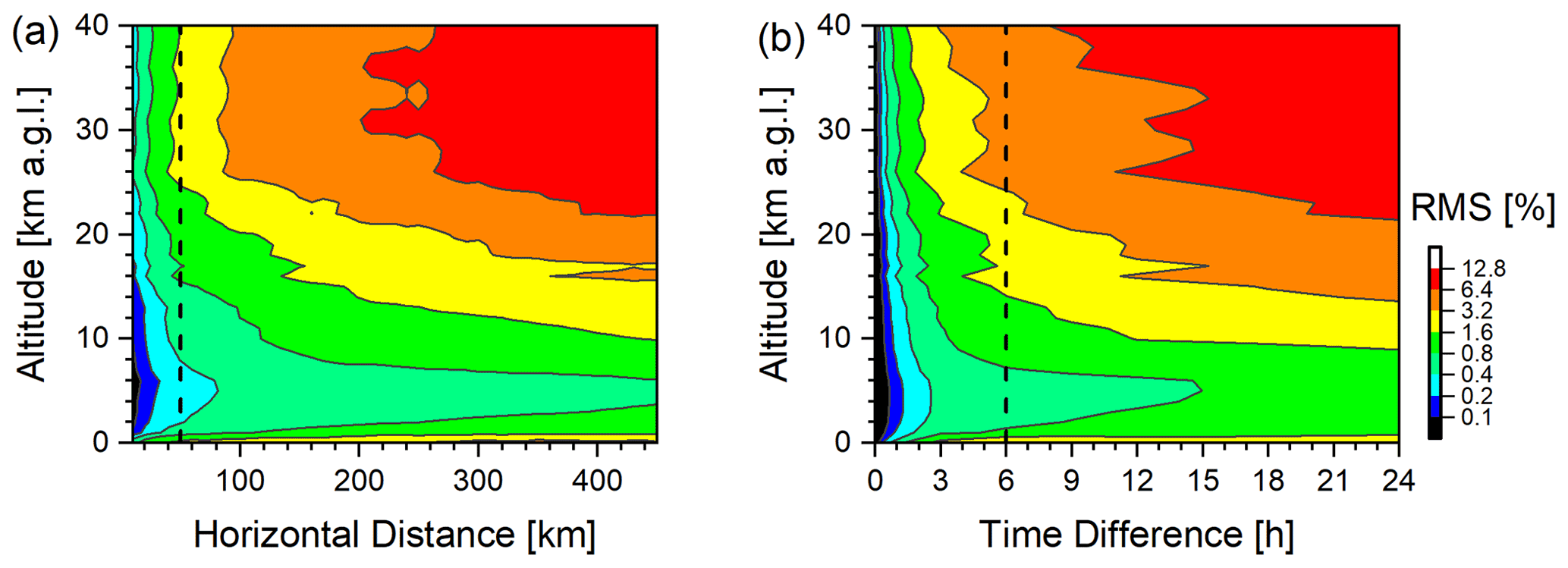
Figure E1Square root values of the diagonal entries of different dislocation covariance matrices (). These values are the root-mean-square (rms) of the difference between the reference methane profile (CAMS forecast for location 49.1∘ N, 8.4∘ E, corresponding to the location of Karlsruhe) and other forecasted profiles dislocated with respect to the reference: (a) horizontal dislocations and (b) temporal dislocations. The dashed black lines indicate the collocation threshold values used for valid combinations of IASI and TROPOMI.
E1 Uncertainty source
For investigating the spatial and temporal variability of the atmospheric CH4 fields, we use the CAMS (Copernicus Atmospheric Monitoring Service; https://atmosphere.copernicus.eu/, last access: 5 July 2022) CH4 forecast product at the highest available resolution (≈9 km; Barré et al., 2021). By analysing the profiles forecasted for the same location but different timestamps, we can determine the temporal covariance of the vertical CH4 fields. Similarly, by analysing the profiles forecasted for the same timestamp but different locations, we get the spatial covariance of the vertical CH4 fields. The analyses are done with CAMS data between November 2017 and December 2020 for central Europe in an area around Karlsruhe. The results are depicted in Figs. E1 to E3.
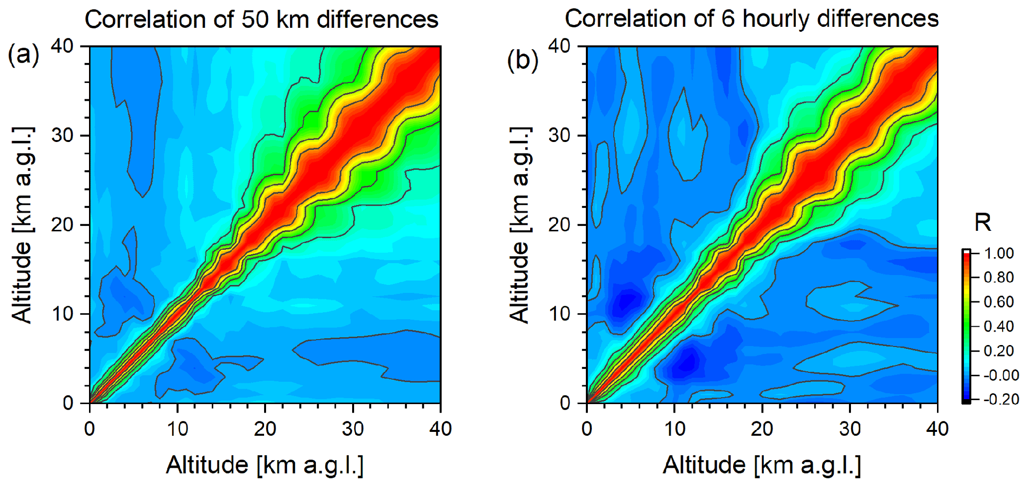
Figure E2Characteristics of the vertical dependencies covered by the matrices . Shown are the vertical correlation matrices for the difference between the reference CH4 profile (location 49.1∘ N, 8.4∘ E, corresponding to the location of Karlsruhe) and profiles dislocated with respect to the reference: (a) horizontal dislocation of 50 km and (b) temporal dislocation of 6 h.
Figure E1 shows the root-mean-square (rms) of the difference between the forecasted reference methane profile and forecasted profiles that are dislocated with respect to the reference by different spatial distances and time differences. These are the square root values of the diagonal entries of the respective dislocation covariance matrices (; we use here the superscript “l” for logarithmic scale because we work with relative covariances: ). The dashed black lines indicate our collocation threshold values used for the combination of TROPOMI and IASI (TROPOMI and IASI are only combined as long as the horizontal distance of their ground pixels is within 50 km, and the time difference is within 6 h). Naturally, the respective rms values increase with increasing horizontal distance and time difference. The values are largest in a small layer close to the surface and in the stratosphere but relatively small in the free troposphere. For a horizontal dislocation of 50 km, the rms value is about 2 % very close to the surface and between 0.3 % and 0.5 % for the rest of the troposphere, and then it increases again to about 2 % above 25 km altitude. For a time difference of 6 h, the rms value is about 2.5 % in a very small layer above the ground and 0.6 %–0.8 % in the free troposphere below 10 km, and it reaches about 1.5 % at 15 km and 3.5 % at 30 km altitude.
Figure E2 reveals to what extent the dislocation uncertainties as shown in Fig. E1 are vertically correlated. Depicted are the vertical correlations for the example of a spatial dislocation of 50 km (Fig. E2a) and a temporal dislocation of 6 h (Fig. E2b). We observe that for both spatial and temporal dislocations, the vertical behaviour of the vertical correlation length (distance where correlation coefficient decays to 0.5) is similar. The vertical correlation lengths are rather short close to the surface (only 100–200 m). They are larger for higher altitudes: in the middle and upper troposphere and in the stratosphere they increase to about 1000 and 6000 m, respectively.

Figure E3Same as Fig. E1 but for column-averaged data: total column, tropospheric partial column, and UTLS partial column.
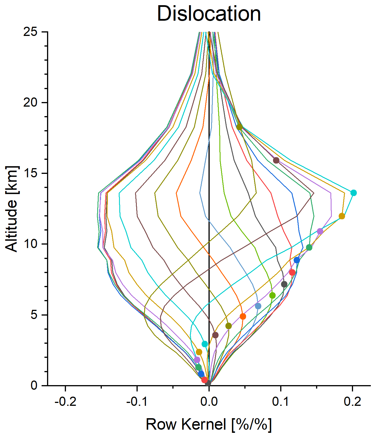
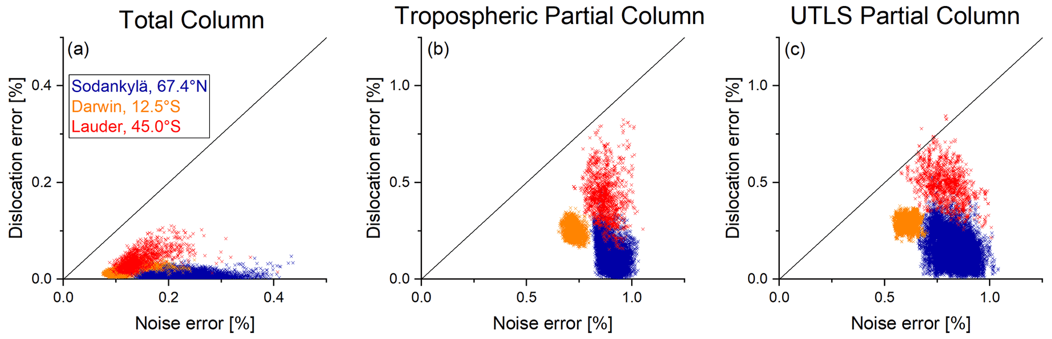
Figure E5Comparison of the dislocation error (due to the CH4 dislocation uncertainty) and the noise error (an example of the typical temporal dependencies of the noise error is shown in Fig. 6). The comparison is depicted for a northern high-latitude location (Sodankylä; violet crosses), a tropical location (Darwin; orange crosses), and a southern middle latitudinal location (Lauder; red crosses). (a) Total-column product, (b) tropospheric partial-column product, and (c) UTLS partial-column product.
The dislocation error for total and partial columns can be calculated by resampling the spatial and temporal dislocation covariance matrices according to Eq. (D7) (for more details, see Appendix D). The results of these resampling calculations are shown for the spatial dislocation in Fig. E3a and for the temporal dislocation in Fig. E3b. Naturally the dislocation uncertainties increase with increasing horizontal distance and time difference. For our horizontal collocation threshold values of 50 km, the uncertainty (rms value is used as the metric) is about 0.2 % for the total-column data. For our time difference collocation threshold of 6 h, it is about 0.3 % for the total-column data. For the tropospheric and upper tropospheric–lower stratospheric partial columns, the respective relative uncertainties values are slightly larger.
E2 Impact on the combined CH4 product
For calculating the error in the combined profile due to the horizontal and spatial dislocation between IASI and TROPOMI, we substitute in Eq. (1) by , where Δdl is the dislocation uncertainty of CH4, as shown in Figs. E1 and E2. This results in a new term in Eq. (1) that gives the dislocation error in the combined profile:
The respective error covariance matrix is
where is the covariance matrix for the CH4 dislocation uncertainty, whose main characteristics are visualized in Figs. E1 and E2. Here,
is the dislocation averaging kernel. Figure E4 shows an example of this dislocation averaging kernel. For the altitudes where the dislocation uncertainty of CH4 is largest (close to the ground and above 20 km; see Fig. E1), the dislocation kernel has rather low values (i.e. there the combination procedure has only limited sensitivity to the dislocation uncertainty).
We calculate the dislocation error covariance matrices according to Eq. (E2) for different locations and then determine the corresponding total- and partial-column dislocation errors by summing up the temporal and spatial dislocation covariances and performing an subsequent resampling of the covariance matrices according to Eq. (D7) (for more details, see Appendix D). Figure E5 depicts this dislocation error in comparison to the noise error (respective resampling of the covariance matrices obtained by Eq. (5); see also Fig. 6). We focus here on three different latitudinal locations: Sodankylä (northern high latitudes), Darwin (low latitudes), and Lauder (southern middle latitudes). We find that for the northern high-latitude site (where horizontal and temporal dislocation are of similar importance) but also for the tropical and southern hemispheric middle-latitude sites (where the temporal dislocation is dominating), the dislocation uncertainty is generally much smaller than the noise error.
The satellite data products are representative of broad vertical layers of the atmosphere (see averaging kernels as shown in Figs. 2 and 3). Also the TCCON and AirCore reference data are sensitive to atmospheric CH4 at different vertical regions. If we furthermore assume that the TCCON and the AirCore data offer a stable absolute calibration reference, their inter-comparisons with the satellite data as shown in Sect. 4 can in principle be used for empirically validating the characteristics (sensitivity and error) of the satellite data products. The level of agreement that can be expected between the reference data and the satellite products depends on the reliability of the references and the characteristics of the satellite data products. In Appendix F1 and F2 we estimate the reliability of the TCCON and AirCore data, respectively, to serve as reference for the satellite data products. Then in Appendix F3 we show that the results of the inter-comparison as shown in the context of Figs. 9 to 12 are in a reasonable agreement with the reliability of the references and the characteristics of the different satellite data products. This confirms the validity of the sensitivity of the satellite data products as shown in Sect. 3.2 and the validity of the errors of the satellite data as documented in Sect. 3.3.
F1 TCCON versus satellite
For estimating the reliability of the TCCON data as reference for the satellite data products we consider the TCCON retrieval noise errors, the incomparableness of TCCON and satellite data caused by their different averaging kernels, and the collocation mismatch between the TCCON and the satellite observations. The total-column uncertainty variance (the scalar ) for using the TCCON data as reference for the satellite data can be estimated by
The first term (the scalar ) is the TCCON retrieval error variance (the TCCON error is provided with the TCCON data is typically 1 ‰). The second term accounts for the different averaging kernels. The row vectors and are the total-column-averaged mixing ratio kernels of the satellite and the TCCON retrievals, respectively (calculated according to Appendix D). The matrix SΔa describes the uncertainty covariances of the a priori data used and the matrices SΔh and SΔt the covariances for horizontal and temporal collocation mismatches.
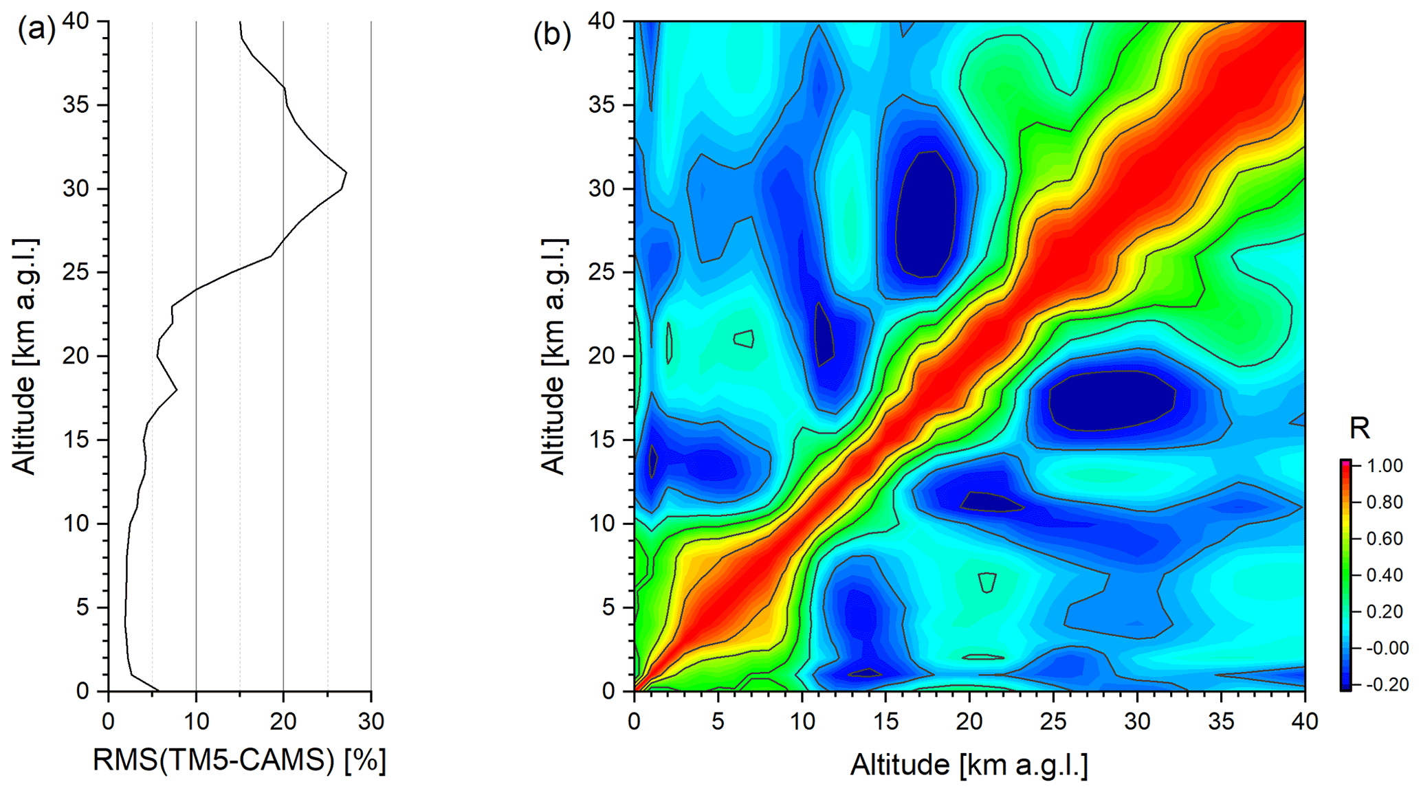
Figure F1Comparison of the CH4 state obtained from the TROPOMI a priori model TM5 (xTM5) and the collocated CAMS high-resolution forecasts (xCAMS). (a) The rms of the relative differences; (b) Matrix showing the correlations of TM5-CAMS differences at different altitudes.
For estimating SΔa we use the difference between the CH4 state as modelled by TM5 (xTM5) and provided by the high-resolution CAMS forecast (xCAMS; e.g. Barré et al., 2021). Figure F1 shows the results of these calculations for the surroundings of Karlsruhe documented by the rms values of the differences in the vertical profiles (Fig. F1a) and the vertical correlation matrix of the differences (Fig. F1b). We estimate an uncertainty of the TM5 a priori model of about 6 % close to the surface, about 2 % up to the middle troposphere, a gradual increase to about 7.5 % between the UTLS and about 23 km altitude, and a maximum value of about 27 % in the stratosphere at about 30 km. The vertical correlation lengths (altitude range where the correlation coefficient decreases to about 0.5) are a few hundred metres close to the surface, about 5000 m in the middle troposphere, about 2500 m in the UTLS, and about 7500 m in the stratosphere above 30 km altitude. We find that this relatively large disagreement between the TM5 a priori data and the high-resolution forecast of CAMS is significantly influenced by inconsistencies between TM5 and CAMS in the years 2019 and 2020: after 2018 the TM5 model shows an increase of about 1 % per year, but the CAMS high-resolution forecast shows no significant increase.
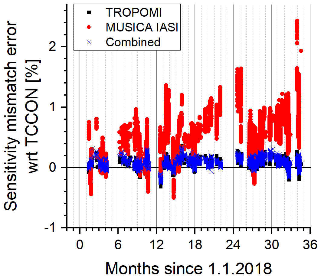
Figure F2Error in the comparison of TCCON and satellite products due to the a priori model error and the different column sensitivities of the TCCON product and the satellite products. These values are calculated as and are represented in Eq. (F1) by the square root value of the term .
Figure F2 shows the value of the term for the different satellite data products; i.e. it reveals the uncertainty in the comparison with TCCON data due to differences in the averaging kernels and the a priori model uncertainty, which in Eq. (F1) is represented by the square root value of the term . Because the TROPOMI and the TCCON kernels both have a similar good column sensitivity throughout the troposphere, the respective uncertainty is generally within 0.1 % (see black squares in Fig. F2). The same is true for the validation of the total column of the combined product (see blue crosses in Fig. F2). For the validation of the total column of the MUSICA IASI product, this error is larger because the total-column sensitivity of IASI is significantly different from the respective sensitivity of the TCCON product and the other satellite products (see Fig. 3a). For the comparison of the IASI and TCCON total-column data, we estimate that the error due to the different sensitivities (of IASI and TCCON) can occasionally be even above 2 % (see red dots in Fig. F2). This error is largest to the end of the time series because then the TM5 a priori model error is largest (increasing difference between the TM5 model and the CAMS high-resolution forecast after 2018).
The collocation mismatch covariances SΔh and SΔt are the linear-scale versions of the matrices (characterized in Figs. E1 and E2) interpolated to the actual temporal and horizontal mismatch of the satellite and the TCCON measurements. The effect of this collocation mismatch on the comparison of the total columns (i.e. the term ) is estimated to be between 0.1 % and 0.4 %.

Figure F3Theoretically predicted and observed 1σ scatter for the comparison of single pixel satellite data with individual TCCON and AirCore reference data. Black, red, and blue colours represent TROPOMI, MUSICA IASI, and combined satellite data, respectively. The squares and vertical crosses are for XCH4 comparisons with TCCON and AirCore references, respectively. The diagonal crosses and stars are for tropospheric and UTLS partial-column comparisons, respectively, with AirCore references.
F2 AirCore versus satellite
Similar to the TCCON data, we estimate the reliability of the AirCore profile data as reference for the satellite observations. For this estimation we consider an AirCore measurement noise covariance (SΔAC,n). It is calculated assuming an uncertainty for altitudes with AirCore CH4 data of 0.3 % (Karion et al., 2010) and the uncertainty according to SΔa from Sect. F1 for all other altitudes. The outer diagonal elements are determined by assuming the same vertical correlation as derived for SΔa. In addition, we consider uncertainties in the height attribution, which is according to Wagenhäuser et al. (2021) below 10 m close to ground, about 200 m at 20 km a.s.l., and about 1 at 27 km a.s.l.
We construct a respective height attribution uncertainty covariance (SΔAC,v) by assuming a very strong correlation of the height attribution uncertainties between different altitude levels. The temporal and spatial collocation mismatch covariance between the AirCore and the satellite observations (SΔh and SΔt, respectively) is calculated as described in Sect. F1.
All the aforementioned uncertainties are independent, and we can calculate the total uncertainty as
The reliability of the AirCore data – after its adjustment according to Eq. (7) – as reference for the MUSICA IASI and combined satellite data can then be estimated by
Here and in Eq. (F2), the covariances are determined for the full vertical profile. Respective covariances for total or partial columns can be derived according to Appendix D. The reliability for the TROPOMI total-column-averaged mixing ratio data can be calculated by .
In order to get a reasonable number of collocated AirCore data, we relax the collocation criteria: we require a temporal collocation within 6 h and a spatial collocation within 500 km (see Sect. 4.2). In particular, a loose spatial collocation requirement results in theoretically large collocation mismatch uncertainties. For instance, Fig. E3 reveals that a spatial mismatch of 400 km clearly dominates the temporal mismatch, whose threshold is set to 6 h, but it is actually only typically greater than 3 h in the Southern Hemisphere. The spatial mismatch uncertainty also dominates the uncertainties in the AirCore data due to measurement noise and uncertain height attribution; i.e. it is the term that most affects the comparability of the AirCore and satellite measurements. We estimate a spatial mismatch error that has to be considered for the AirCore satellite inter-comparison of about 0.5 % for the total-column data and of about 0.6 % for the tropospheric and UTLS partial-column data.
F3 Summary
The sum of the uncertainty (co)variance of using TCCON or AirCore as the reference ( or ; see Sects. F1 and F2, respectively) and the noise and dislocation error (co)variances of the satellite data products (see Sects. 3.3 and 3.4, respectively) gives the covariance that can be theoretically expected for the scatter between the TCCON or AirCore reference data and the satellite data products.
Figure F3 shows the correlations between the theoretically expected scatter (mean value of the scatter expected for the individual data points) and the actually observed scatter (the hIPR68.2 of the individual differences between the reference data and the satellite data products). Shown is one data point for the XCH4 comparisons with the TCCON references, for the XCH4 comparisons with the AirCore references, and further data points for the comparisons of the tropospheric and UTLS partial columns with the AirCore references. A detailed contemplation suggests that the scatter observed for the total-column data of the TROPOMI and the combined data products, as well as the scatter observed for the tropospheric partial-column data of the IASI and combined products, is slightly larger than their theoretically expected counterparts. Conversely, in the UTLS the scatter observed in the IASI and combined data products seems to be a bit smaller than the theoretically expected scatter values. However, the data points group reasonably well around the one-to-one diagonal; i.e. there is overall a good agreement between the theoretically expected scatter and the actually observed scatter. This means that the inter-comparison results as shown in Sect. 4 confirm the satellite data quality characterization of Sects. 3.2–3.4.
The MUSICA IASI data are described in (Schneider et al., 2022) and can be accessed at https://doi.org/10.35097/408 (Schneider et al., 2021a) and https://doi.org/10.35097/412 (Schneider et al., 2021b). The TROPOMI XCH4 data used in this study are described in Lorente et al. (2021a) and can be accessed at https://doi.org/10.5281/zenodo.4447228 (Lorente et al., 2021b). The TCCON data are available via the TCCON data archive, hosted by CaltechDATA (Total Carbon Column Observing Network Team, 2014, https://doi.org/10.14291/TCCON.GGG2014). For Trainou AirCore data, please contact Michel Ramonet (michel.ramonet@lsce.ipsl.fr), and for Sodankylä AirCore data, please contact Huilin Chen (huilin.chen@rug.nl). The Jungfraujoch GAW surface in situ CH4 data are available via the World Data Centre for Greenhouse Gases (WDCGG) and can be directly accessed at https://doi.org/10.50849/WDCGG_0023-6036-1002-01-01-9999 (Steinbacher, 2022). The Schainsland GAW surface in situ CH4 data up to 31 December 2018 are available via the WDCGG at https://gaw.kishou.go.jp/search/station#SSL (Meinhardt, 2019). For the Schauinsland CH4 data for 2019 and 2020, please contact Frank Meinhardt (frank.meinhardt@uba.de). The fused “MUSICA IASI/RemoTeC TROPOMI” example data presented in Fig. 15 are accessible at https://doi.org/10.35097/689 (Schneider and Ertl, 2022a). As already stated in Sect. 2.1, in this work we use the TROPOMI XCH4 data generated by the operational processing algorithm version 2.2.0 as input for the data fusion. For the example months of Fig. 15, we make additional data fusion calculations using the TROPOMI CH4 operational processing algorithm version 2.3.1, which among others offers additional coverage over ocean using glint mode observations. These fused “MUSICA IASI/RemoTeC TROPOMI” data are accessible at https://doi.org/10.35097/690 (Schneider and Ertl, 2022b).
MSc developed the idea for the optimal a posteriori combination of the level 2 remote-sensing products, and he prepared the figures and the manuscript. BE developed and performed the continuous MUSICA IASI data processing, where he was supported by MSc, CJD, FK, ANR, OEG, and ES. FH developed the PROFFIT-nadir retrieval code used for the MUSICA IASI processing. QT supported the use of the CAMS high-resolution data. TB, JL, AL, and AB are responsible for the TROPOMI processing and for making TROPOMI data available. HC and RK are responsible for the AirCore profile measurements over Sodankylä. TL, MR, CC, and JP are responsible for the AirCore profile measurements over Trainou. MSt and FM are responsible for the GAW data of Jungfraujoch and Schauinsland, respectively. RK, DD, FH, KSt, DW, TW, CR, POW, IM, LTI, KSh, NMD, DWTG, VAV, and DFP are responsible for the TCCON data. All authors supported the generation of the final version of this paper.
The contact author has declared that neither they nor their co-authors have any competing interests.
Publisher's note: Copernicus Publications remains neutral with regard to jurisdictional claims in published maps and institutional affiliations.
This research has largely benefitted from funds of the Deutsche Forschungsgemeinschaft (provided for the two projects MOTIV and TEDDY with IDs/Geschäftszeichen 290612604/GZ:SCHN1126/2-1 and 416767181/GZ:SCHN1126/5-1, respectively) and from support by the European Space Agency in the context the “Sentinel-5p+Innovation (S5p+I) – Water Vapour Isotopologues (H2O-ISO)” activities. Furthermore, we acknowledge funds from the Ministerio de Economía y Competividad from Spain for the project INMENSE (CGL2016-80688-P).
An important part of this work was performed on the supercomputers ForHLR and HoreKa funded by the Ministry of Science, Research and the Arts Baden-Württemberg and by the German Federal Ministry of Education and Research. We also acknowledge the contribution of Teide High-Performance Computing facilities. Teide HPC facilities are provided by the Instituto Tecnológico y de Energías Renovables (ITER), S.A (https://teidehpc.iter.es/en/home/, last access: 5 July 2022).
The TROPOMI data processing was carried out on the Dutch National e-Infrastructure with the support of the SURF cooperative. The presented material contains modified Copernicus data (2017, 2019).
The Eureka TCCON measurements were made at the Polar Environment Atmospheric Research Laboratory (PEARL) by the Canadian Network for the Detection of Atmospheric Change, primarily supported by NSERC, ECCC, and CSA. The East Trout Lake TCCON station is supported by CFI, ORF, and NSERC. The Karlsruhe TCCON station has been supported by the German Bundesministerium für Wirtschaft und Energie (BMWi) via DLR under grants 50EE1711A to E and by the Helmholtz Society via the research program ATMO. The Park Falls and Lamont TCCON sites are supported by and would like to acknowledge NASA's Carbon Cycle Science Program (grant no. NNX17AE15G) and OCO-2 and OCO-3 projects (primary grant no. NNN12AA01C), respectively. The Burgos and Rikubetsu TCCON sites are supported in part by the GOSAT series project. Burgos is supported in part by the Energy Development Corp., the Philippines. Funding for the Edwards TCCON station is provided by NASA's Earth Science Division. Nicholas M. Deutscher is funded by ARC Future Fellowship FT180100327. Darwin and Wollongong TCCON stations are supported by ARC grants DP160100598, LE0668470, DP140101552, DP110103118, and DP0879468 and Darwin through NASA grants NAG5-12247 and NNG05-GD07G. The Lauder TCCON programme is core-funded by NIWA through New Zealand's Ministry of Business, Innovation and Employment.
The Trainou AirCore measurements have been supported by CEA, CNES, UVSQ, IPSL, and the EU H2020 RINGO project (GA no. 730944) and are part of the French consortium for Aircore measurements (LMD, LSCE, GSMA, CNES). The Sodankylä TCCON and AirCore measurements have been supported via the ESA FRM4GHG project (under grant agreement no. ESA-IPLPOE-LG-cl-LE-2015-1129) and the EU H2020 RINGO project.
The CH4 observations at Jungfraujoch were established as part of the Swiss National Air Pollution Monitoring Network and are supported through ICOS-CH, which is funded by the Swiss National Science Foundation and in-house contributions.
We would like to thank our colleague Thomas von Clarmann for his strong support in revising the equations in the Appendix of this paper.
We thank Michela Giusti in the Data Support team at ECMWF for retrieving and providing comments about the CAMS data.
We acknowledge the support by the Deutsche Forschungsgemeinschaft and the Open Access Publishing Fund of the Karlsruhe Institute of Technology.
This research has been supported by the Deutsche Forschungsgemeinschaft (project MOTIV (grant no. 290612604), and project TEDDY (grant no. 416767181)), the Ministerio de Economía y Competitividad (grant no. CGL2016-80688-P), the European Space Agency (grant nos. 4000127561/19/I-NS and ESA-IPLPOE-LG-cl-LE-2015-1129), the Ministerium für Wissenschaft, Forschung und Kunst Baden-Württemberg, and the Bundesministerium für Bildung und Forschung for funding in the context of the ForHLR and HoreKa supercomputing infrastructure.
The article processing charges for this open-access publication were covered by the Karlsruhe Institute of Technology (KIT).
This paper was edited by John Worden and reviewed by Thomas von Clarmann and two anonymous referees.
Barré, J., Aben, I., Agustí-Panareda, A., Balsamo, G., Bousserez, N., Dueben, P., Engelen, R., Inness, A., Lorente, A., McNorton, J., Peuch, V.-H., Radnoti, G., and Ribas, R.: Systematic detection of local CH4 anomalies by combining satellite measurements with high-resolution forecasts, Atmos. Chem. Phys., 21, 5117–5136, https://doi.org/10.5194/acp-21-5117-2021, 2021. a, b
Borger, C., Schneider, M., Ertl, B., Hase, F., García, O. E., Sommer, M., Höpfner, M., Tjemkes, S. A., and Calbet, X.: Evaluation of MUSICA IASI tropospheric water vapour profiles using theoretical error assessments and comparisons to GRUAN Vaisala RS92 measurements, Atmos. Meas. Tech., 11, 4981–5006, https://doi.org/10.5194/amt-11-4981-2018, 2018. a
Butz, A., Guerlet, S., Hasekamp, O., Schepers, D., Galli, A., Aben, I., Frankenberg, C., Hartmann, J.-M., Tran, H., Kuze, A., Keppel-Aleks, G., Toon, G., Wunch, D., Wennberg, P., Deutscher, N., Griffith, D., Macatangay, R., Messerschmidt, J., Notholt, J., and Warneke, T.: Toward accurate CO2 and CH4 observations from GOSAT, Geophys. Res. Lett., 38, L14812, https://doi.org/10.1029/2011GL047888, 2011. a
Ceccherini, S., Raspollini, P., and Carli, B.: Optimal use of the information provided by indirect measurements of atmospheric vertical profiles, Opt. Express, 17, 4944–4958, https://doi.org/10.1364/OE.17.004944, 2009. a
Cortesi, U., Del Bianco, S., Ceccherini, S., Gai, M., Dinelli, B. M., Castelli, E., Oelhaf, H., Woiwode, W., Höpfner, M., and Gerber, D.: Synergy between middle infrared and millimeter-wave limb sounding of atmospheric temperature and minor constituents, Atmos. Meas. Tech., 9, 2267–2289, https://doi.org/10.5194/amt-9-2267-2016, 2016. a
Costantino, L., Cuesta, J., Emili, E., Coman, A., Foret, G., Dufour, G., Eremenko, M., Chailleux, Y., Beekmann, M., and Flaud, J.-M.: Potential of multispectral synergism for observing ozone pollution by combining IASI-NG and UVNS measurements from the EPS-SG satellite, Atmos. Meas. Tech., 10, 1281–1298, https://doi.org/10.5194/amt-10-1281-2017, 2017. a
Cuesta, J., Eremenko, M., Liu, X., Dufour, G., Cai, Z., Höpfner, M., von Clarmann, T., Sellitto, P., Foret, G., Gaubert, B., Beekmann, M., Orphal, J., Chance, K., Spurr, R., and Flaud, J.-M.: Satellite observation of lowermost tropospheric ozone by multispectral synergism of IASI thermal infrared and GOME-2 ultraviolet measurements over Europe, Atmos. Chem. Phys., 13, 9675–9693, https://doi.org/10.5194/acp-13-9675-2013, 2013. a, b
Diekmann, C. J., Schneider, M., Ertl, B., Hase, F., García, O., Khosrawi, F., Sepúlveda, E., Knippertz, P., and Braesicke, P.: The global and multi-annual MUSICA IASI {H2O, δ D} pair dataset, Earth Syst. Sci. Data, 13, 5273–5292, https://doi.org/10.5194/essd-13-5273-2021, 2021. a
Fu, D., Worden, J. R., Liu, X., Kulawik, S. S., Bowman, K. W., and Natraj, V.: Characterization of ozone profiles derived from Aura TES and OMI radiances, Atmos. Chem. Phys., 13, 3445–3462, https://doi.org/10.5194/acp-13-3445-2013, 2013. a
García, O. E., Schneider, M., Ertl, B., Sepúlveda, E., Borger, C., Diekmann, C., Wiegele, A., Hase, F., Barthlott, S., Blumenstock, T., Raffalski, U., Gómez-Peláez, A., Steinbacher, M., Ries, L., and de Frutos, A. M.: The MUSICA IASI CH4 and N2O products and their comparison to HIPPO, GAW and NDACC FTIR references, Atmos. Meas. Tech., 11, 4171–4215, https://doi.org/10.5194/amt-11-4171-2018, 2018. a
Griffith, D. W., Deutscher, N. M., Velazco, V. A., Wennberg, P. O., Yavin, Y., Keppel-Aleks, G., Washenfelder, R. A., Toon, G. C., Blavier, J.-F., Paton-Walsh, C., Jones, N. B., Kettlewell, G. C., Connor, B. J., Macatangay, R. C., Roehl, C., Ryczek, M., Glowacki, J., Culgan, T., and Bryant, G. W.: TCCON data from Darwin (AU), Release GGG2014.R0, CaltechDATA [data set], https://doi.org/10.14291/TCCON.GGG2014.DARWIN01.R0/1149290, 2014a. a
Griffith, D. W., Velazco, V. A., Deutscher, N. M., Paton-Walsh, C., Jones, N. B., Wilson, S. R., Macatangay, R. C., Kettlewell, G. C., Buchholz, R. R., and Riggenbach, M. O.: TCCON data from Wollongong (AU), Release GGG2014.R0, CaltechDATA [data set], https://doi.org/10.14291/TCCON.GGG2014.WOLLONGONG01.R0/1149291, 2014b. a
Hase, F., Blumenstock, T., Dohe, S., Groß, J., and Kiel, M.: TCCON data from Karlsruhe (DE), Release GGG2014.R1, CaltechDATA [data set], https://doi.org/10.14291/TCCON.GGG2014.KARLSRUHE01.R1/1182416, 2015. a
Hasekamp, O., Lorente, A., Hu, H., Butz, A., aan de Brugh, J., and Landgraf, J.: Algorithm Theoretical Baseline Document for Senitinel-5 Precursor methane retrieval, https://sentinel.esa.int/documents/247904/2476257/Sentinel-5P-TROPOMI-ATBD-Methane-retrieval (last access: 5 July 2022), 2021. a
Hu, H., Hasekamp, O., Butz, A., Galli, A., Landgraf, J., Aan de Brugh, J., Borsdorff, T., Scheepmaker, R., and Aben, I.: The operational methane retrieval algorithm for TROPOMI, Atmos. Meas. Tech., 9, 5423–5440, https://doi.org/10.5194/amt-9-5423-2016, 2016. a
Iraci, L. T., Podolske, J. R., Hillyard, P. W., Roehl, C., Wennberg, P. O., Blavier, J.-F., Landeros, J., Allen, N., Wunch, D., Zavaleta, J., Quigley, E., Osterman, G. B., Albertson, R., Dunwoody, K., and Boyden, H.: TCCON data from Edwards (US), Release GGG2014.R1, CaltechDATA [data set], https://doi.org/10.14291/TCCON.GGG2014.EDWARDS01.R1/1255068, 2016. a
Kalman, R. E.: A New Approach to Linear Filtering and Prediction Problems, J. Basic Eng.-T. ASME, 82, 35–45, https://doi.org/10.1115/1.3662552, 1960. a
Karion, A., Sweeney, C., Tans, P., and Newberger, T.: AirCore: An Innovative Atmospheric Sampling System, J. Atmos. Ocean. Tech., 27, 1839–1853, https://doi.org/10.1175/2010JTECHA1448.1, 2010. a, b, c
Kawakami, S., Ohyama, H., Arai, K., Okumura, H., Taura, C., Fukamachi, T., and Sakashita, M.: TCCON data from Saga (JP), Release GGG2014.R0, CaltechDATA [data set], https://doi.org/10.14291/TCCON.GGG2014.SAGA01.R0/1149283, 2014. a
Keppens, A., Lambert, J.-C., Granville, J., Miles, G., Siddans, R., van Peet, J. C. A., van der A, R. J., Hubert, D., Verhoelst, T., Delcloo, A., Godin-Beekmann, S., Kivi, R., Stübi, R., and Zehner, C.: Round-robin evaluation of nadir ozone profile retrievals: methodology and application to MetOp-A GOME-2, Atmos. Meas. Tech., 8, 2093–2120, https://doi.org/10.5194/amt-8-2093-2015, 2015. a
Kivi, R. and Heikkinen, P.: Fourier transform spectrometer measurements of column CO2 at Sodankylä, Finland, Geosci. Instrum. Meth., 5, 271–279, https://doi.org/10.5194/gi-5-271-2016, 2016. a
Kivi, R., Heikkinen, P., and Kyrö, E.: TCCON data from Sodankylä (FI), Release GGG2014.R0, CaltechDATA [data set], https://doi.org/10.14291/TCCON.GGG2014.SODANKYLA01.R0/1149280, 2014. a
Krol, M., Houweling, S., Bregman, B., van den Broek, M., Segers, A., van Velthoven, P., Peters, W., Dentener, F., and Bergamaschi, P.: The two-way nested global chemistry-transport zoom model TM5: algorithm and applications, Atmos. Chem. Phys., 5, 417–432, https://doi.org/10.5194/acp-5-417-2005, 2005. a, b
Landgraf, J. and Hasekamp, O. P.: Retrieval of tropospheric ozone: The synergistic use of thermal infrared emission and ultraviolet reflectivity measurements from space, J. Geophys. Res.-Atmos., 112, D08310, https://doi.org/10.1029/2006JD008097, 2007. a
Lorente, A., Borsdorff, T., Butz, A., Hasekamp, O., aan de Brugh, J., Schneider, A., Wu, L., Hase, F., Kivi, R., Wunch, D., Pollard, D. F., Shiomi, K., Deutscher, N. M., Velazco, V. A., Roehl, C. M., Wennberg, P. O., Warneke, T., and Landgraf, J.: Methane retrieved from TROPOMI: improvement of the data product and validation of the first 2 years of measurements, Atmos. Meas. Tech., 14, 665–684, https://doi.org/10.5194/amt-14-665-2021, 2021a. a, b, c, d, e, f
Lorente, A., Borsdorff, T., aan de Brugh, J., Landgraf, J., and Hasekamp, O.: SRON S5P – RemoTeC scientific TROPOMI XCH4 dataset, Zenodo [data set], https://doi.org/10.5281/zenodo.4447228, 2021b a
Luo, M., Read, W., Kulawik, S., Worden, J., Livesey, N., Bowman, K., and Herman, R.: Carbon monoxide (CO) vertical profiles derived from joined TES and MLS measurements, J. Geophys. Res.-Atmos., 118, 10601–10613, https://doi.org/10.1002/jgrd.50800, 2013. a
Meinhardt, F.: Atmospheric CH4 at Schauinsland by German Environment Agency, ch4_ssl_surface-insitu_71_9999-9999_hourly, dataset version: 0071-6027-1002-01-01-9999_2019-06-07-1841, WDCGG [data set], https://gaw.kishou.go.jp/search/station#SSL (last access: 11 July 2022), 2019. a
Morino, I., Yokozeki, N., Matsuzaki, T., and Horikawa, M.: TCCON data from Rikubetsu (JP), Release GGG2014.R2, CaltechDATA [data set], https://doi.org/10.14291/TCCON.GGG2014.RIKUBETSU01.R2, 2018. a
Pandey, S., Houweling, S., Krol, M., Aben, I., Chevallier, F., Dlugokencky, E. J., Gatti, L. V., Gloor, E., Miller, J. B., Detmers, R., Machida, T., and Röckmann, T.: Inverse modeling of GOSAT-retrieved ratios of total column CH4 and CO2 for 2009 and 2010, Atmos. Chem. Phys., 16, 5043–5062, https://doi.org/10.5194/acp-16-5043-2016, 2016. a
Parker, R. J., Webb, A., Boesch, H., Somkuti, P., Barrio Guillo, R., Di Noia, A., Kalaitzi, N., Anand, J. S., Bergamaschi, P., Chevallier, F., Palmer, P. I., Feng, L., Deutscher, N. M., Feist, D. G., Griffith, D. W. T., Hase, F., Kivi, R., Morino, I., Notholt, J., Oh, Y.-S., Ohyama, H., Petri, C., Pollard, D. F., Roehl, C., Sha, M. K., Shiomi, K., Strong, K., Sussmann, R., Té, Y., Velazco, V. A., Warneke, T., Wennberg, P. O., and Wunch, D.: A decade of GOSAT Proxy satellite CH4 observations, Earth Syst. Sci. Data, 12, 3383–3412, https://doi.org/10.5194/essd-12-3383-2020, 2020. a
Pollard, D. F., Robinson, J., and Shiona, H.: TCCON data from Lauder (NZ), Release GGG2014.R0, CaltechDATA [data set], https://doi.org/10.14291/TCCON.GGG2014.LAUDER03.R0, 2019. a
Rodgers, C.: Inverse Methods for Atmospheric Sounding: Theory and Praxis, Series on Atmospheric, Oceanic and Planetary Physics – Vol. 2, edited by: Taylor, F. W., University of Oxford, World Scientific Publishing Co., Singapore, ISBN 981-02-2740-X, 2000. a, b, c, d, e, f, g, h, i, j, k
Rodgers, C. and Connor, B.: Intercomparison of remote sounding instruments, J. Geophys. Res., 108, 4116–4129, https://doi.org/10.1029/2002JD002299, 2003. a, b, c
Schneider, M. and Ertl, B.: MUSICA IASI/RemoTeC TROPOMI fused methane data set (version 1.0), KIT [data set], https://doi.org/10.35097/689, 2022a. a
Schneider, M. and Ertl, B.: MUSICA IASI/RemoTeC TROPOMI fused methane data set (version 2.0), KIT [data set], https://doi.org/10.35097/690, 2022b. a
Schneider, M., Wiegele, A., Barthlott, S., González, Y., Christner, E., Dyroff, C., García, O. E., Hase, F., Blumenstock, T., Sepúlveda, E., Mengistu Tsidu, G., Takele Kenea, S., Rodríguez, S., and Andrey, J.: Accomplishments of the MUSICA project to provide accurate, long-term, global and high-resolution observations of tropospheric {H2O,δD} pairs – a review, Atmos. Meas. Tech., 9, 2845–2875, https://doi.org/10.5194/amt-9-2845-2016, 2016. a
Schneider, M., Ertl, B., and Diekmann, C.: MUSICA IASI full retrieval product standard output (processing version 3.2.1), KIT [data set], https://doi.org/10.35097/408, 2021a. a
Schneider, M., Ertl, B., and Diekmann, C.: MUSICA IASI full retrieval product extended output (processing version 3.2.1), KIT [data set], https://doi.org/10.35097/412, 2021b. a
Schneider, M., Ertl, B., Diekmann, C. J., Khosrawi, F., Weber, A., Hase, F., Höpfner, M., García, O. E., Sepúlveda, E., and Kinnison, D.: Design and description of the MUSICA IASI full retrieval product, Earth Syst. Sci. Data, 14, 709–742, https://doi.org/10.5194/essd-14-709-2022, 2022. a, b, c, d, e
Sepúlveda, E., Schneider, M., Hase, F., Barthlott, S., Dubravica, D., García, O. E., Gomez-Pelaez, A., González, Y., Guerra, J. C., Gisi, M., Kohlhepp, R., Dohe, S., Blumenstock, T., Strong, K., Weaver, D., Palm, M., Sadeghi, A., Deutscher, N. M., Warneke, T., Notholt, J., Jones, N., Griffith, D. W. T., Smale, D., Brailsford, G. W., Robinson, J., Meinhardt, F., Steinbacher, M., Aalto, T., and Worthy, D.: Tropospheric CH4 signals as observed by NDACC FTIR at globally distributed sites and comparison to GAW surface in situ measurements, Atmos. Meas. Tech., 7, 2337–2360, https://doi.org/10.5194/amt-7-2337-2014, 2014. a, b
Sha, M. K., Langerock, B., Blavier, J.-F. L., Blumenstock, T., Borsdorff, T., Buschmann, M., Dehn, A., De Mazière, M., Deutscher, N. M., Feist, D. G., García, O. E., Griffith, D. W. T., Grutter, M., Hannigan, J. W., Hase, F., Heikkinen, P., Hermans, C., Iraci, L. T., Jeseck, P., Jones, N., Kivi, R., Kumps, N., Landgraf, J., Lorente, A., Mahieu, E., Makarova, M. V., Mellqvist, J., Metzger, J.-M., Morino, I., Nagahama, T., Notholt, J., Ohyama, H., Ortega, I., Palm, M., Petri, C., Pollard, D. F., Rettinger, M., Robinson, J., Roche, S., Roehl, C. M., Röhling, A. N., Rousogenous, C., Schneider, M., Shiomi, K., Smale, D., Stremme, W., Strong, K., Sussmann, R., Té, Y., Uchino, O., Velazco, V. A., Vigouroux, C., Vrekoussis, M., Wang, P., Warneke, T., Wizenberg, T., Wunch, D., Yamanouchi, S., Yang, Y., and Zhou, M.: Validation of methane and carbon monoxide from Sentinel-5 Precursor using TCCON and NDACC-IRWG stations, Atmos. Meas. Tech., 14, 6249–6304, https://doi.org/10.5194/amt-14-6249-2021, 2021. a, b
Sherlock, V., Connor, B., Robinson, J., Shiona, H., Smale, D., and Pollard, D. F.: TCCON data from Lauder (NZ), 125HR, Release GGG2014.R0, CaltechDATA [data set], https://doi.org/10.14291/TCCON.GGG2014.LAUDER02.R0/1149298, 2014. a
Steinbacher, M.: Atmospheric CH4 at Jungfraujoch by Swiss Federal Laboratories for Materials Science and Technology (Empa), dataset published as CH4_JFJ_surface-insitu_Empa_data1 at WDCGG, ver. 2022-07-06-1450, https://doi.org/10.50849/WDCGG_0023-6036-1002-01-01-9999 (Reference date: 11 July 2022), 2022. a
Strong, K., Roche, S., Franklin, J. E., Mendonca, J., Lutsch, E., Weaver, D., Fogal, P. F., Drummond, J. R., Batchelor, R., and Lindenmaier, R.: TCCON data from Eureka (CA), Release GGG2014.R3, CaltechDATA [data set], https://doi.org/10.14291/TCCON.GGG2014.EUREKA01.R3, 2019. a
Total Carbon Column Observing Network (TCCON) Team: 2014 TCCON Data Release, Version GGG2014, CaltechDATA [data set], https://doi.org/10.14291/TCCON.GGG2014, 2017. a
Velazco, V. A., Morino, I., Uchino, O., Hori, A., Kiel, M., Bukosa, B., Deutscher, N. M., Sakai, T., Nagai, T., Bagtasa, G., Izumi, T., Yoshida, Y., and Griffith, D. W. T.: TCCON Philippines: First Measurement Results, Satellite Data and Model Comparisons in Southeast Asia, Remote Sensing, 9, 1228, https://doi.org/10.3390/rs9121228, 2017. a
von Clarmann, T., Degenstein, D. A., Livesey, N. J., Bender, S., Braverman, A., Butz, A., Compernolle, S., Damadeo, R., Dueck, S., Eriksson, P., Funke, B., Johnson, M. C., Kasai, Y., Keppens, A., Kleinert, A., Kramarova, N. A., Laeng, A., Langerock, B., Payne, V. H., Rozanov, A., Sato, T. O., Schneider, M., Sheese, P., Sofieva, V., Stiller, G. P., von Savigny, C., and Zawada, D.: Overview: Estimating and reporting uncertainties in remotely sensed atmospheric composition and temperature, Atmos. Meas. Tech., 13, 4393–4436, https://doi.org/10.5194/amt-13-4393-2020, 2020. a
Wagenhäuser, T., Engel, A., and Sitals, R.: Testing the altitude attribution and vertical resolution of AirCore measurements with a new spiking method, Atmos. Meas. Tech., 14, 3923–3934, https://doi.org/10.5194/amt-14-3923-2021, 2021. a
Warneke, T., Messerschmidt, J., Notholt, J., Weinzierl, C., Deutscher, N. M., Petri, C., and Grupe, P.: TCCON data from Orléans (FR), Release GGG2014.R1, CaltechDATA [data set], https://doi.org/10.14291/TCCON.GGG2014.ORLEANS01.R1, 2019. a
Warner, J. X., Yang, R., Wei, Z., Carminati, F., Tangborn, A., Sun, Z., Lahoz, W., Attié, J.-L., El Amraoui, L., and Duncan, B.: Global carbon monoxide products from combined AIRS, TES and MLS measurements on A-train satellites, Atmos. Chem. Phys., 14, 103–114, https://doi.org/10.5194/acp-14-103-2014, 2014. a
Wennberg, P. O., Wunch, D., Roehl, C. M., Blavier, J.-F., Toon, G. C., and Allen, N. T.: TCCON data from Lamont (US), Release GGG2014.R1, CaltechDATA [data set], https://doi.org/10.14291/TCCON.GGG2014.LAMONT01.R1/1255070, 2016. a
Wennberg, P. O., Roehl, C. M., Wunch, D., Toon, G. C., Blavier, J.-F., Washenfelder, R., Keppel-Aleks, G., Allen, N. T., and Ayers, J.: TCCON data from Park Falls (US), Release GGG2014.R1, CaltechDATA [data set], https://doi.org/10.14291/TCCON.GGG2014.PARKFALLS01.R1, 2017. a
Worden, J., Liu, X., Bowman, K., Chance, K., Beer, R., Eldering, A., Gunson, M., and Worden, H.: Improved tropospheric ozone profile retrievals using OMI and TES radiances, Geophys. Res. Lett., 34, L01809, https://doi.org/10.1029/2006GL027806, 2007. a
Worden, J. R., Turner, A. J., Bloom, A., Kulawik, S. S., Liu, J., Lee, M., Weidner, R., Bowman, K., Frankenberg, C., Parker, R., and Payne, V. H.: Quantifying lower tropospheric methane concentrations using GOSAT near-IR and TES thermal IR measurements, Atmos. Meas. Tech., 8, 3433–3445, https://doi.org/10.5194/amt-8-3433-2015, 2015. a
Wunch, D., Toon, G. C., Blavier, J.-F. L., Washenfelder, R. A., Notholt, J., Connor, B. J., Griffith, D. W. T., Sherlock, V., and Wennberg, P. O.: The Total Carbon Column Observing Network, Philos. T. R. Soc. A., 369, 2087–2112, https://doi.org/10.1098/rsta.2010.0240, 2011a. a
Wunch, D., Wennberg, P. O., Toon, G. C., Connor, B. J., Fisher, B., Osterman, G. B., Frankenberg, C., Mandrake, L., O'Dell, C., Ahonen, P., Biraud, S. C., Castano, R., Cressie, N., Crisp, D., Deutscher, N. M., Eldering, A., Fisher, M. L., Griffith, D. W. T., Gunson, M., Heikkinen, P., Keppel-Aleks, G., Kyrö, E., Lindenmaier, R., Macatangay, R., Mendonca, J., Messerschmidt, J., Miller, C. E., Morino, I., Notholt, J., Oyafuso, F. A., Rettinger, M., Robinson, J., Roehl, C. M., Salawitch, R. J., Sherlock, V., Strong, K., Sussmann, R., Tanaka, T., Thompson, D. R., Uchino, O., Warneke, T., and Wofsy, S. C.: A method for evaluating bias in global measurements of CO2 total columns from space, Atmos. Chem. Phys., 11, 12317–12337, https://doi.org/10.5194/acp-11-12317-2011, 2011b. a
Wunch, D., Mendonca, J., Colebatch, O., Allen, N. T., Blavier, J.-F., Roche, S., Hedelius, J., Neufeld, G., Springett, S., Worthy, D., Kessler, R., and Strong, K.: TCCON data from East Trout Lake, SK (CA), Release GGG2014.R1, CaltechDATA [data set], https://doi.org/10.14291/TCCON.GGG2014.EASTTROUTLAKE01.R1, 2018. a
- Abstract
- Introduction
- Satellite data
- Presentation and characterization of the combination method
- Validation
- Global data
- Summary and outlook
- Appendix A: Basics on retrieval theory
- Appendix B: Theory on the optimal combination of retrieval data products
- Appendix C: Operator for transformation between linear and logarithmic scales
- Appendix D: Operators for column data
- Appendix E: Dislocation of TROPOMI and IASI
- Appendix F: Data comparability
- Data availability
- Author contributions
- Competing interests
- Disclaimer
- Acknowledgements
- Financial support
- Review statement
- References