The Space Carbon Observatory (SCARBO) concept: assessment of X_CO2 and X_CH4 retrieval performance

Several single-platform satellite missions have been designed during the past decades in order to retrieve the atmospheric concentrations of anthropogenic greenhouse gases (GHG), initiating worldwide efforts towards better monitoring of their sources and sinks. To set up a future operational system for anthropogenic GHG emission monitoring, both revisit frequency and spatial resolution need to be improved. The Space Carbon Observatory (SCARBO) project aims at significantly increasing the revisit frequency of spaceborne GHG measurements, while reaching state-of-the-art precision requirements, by implementing a concept of small satellite constellation. It would accommodate a miniaturised GHG sensor named NanoCarb coupled with an aerosol instrument, the multi-angle polarimeter SPEXone. More specifically, the NanoCarb sensor is a static Fabry–Pérot imaging interferometer with a 2.3×2.3 km² spatial resolution and 200 km swath. It samples a truncated interferogram at optical path differences (OPDs) optimally sensitive to all the geophysical parameters necessary to retrieve column-averaged dry-air mole fractions of CO₂ and CH₄ (hereafter $X_{{\mathrm{CO}}_{\mathrm{2}}}$ and $X_{{\mathrm{CH}}_{\mathrm{4}}}$). In this work, we present the Level 2 performance assessment of the concept proposed in the SCARBO project. We perform inverse radiative transfer to retrieve $X_{{\mathrm{CO}}_{\mathrm{2}}}$ and $X_{{\mathrm{CH}}_{\mathrm{4}}}$ directly from synthetic NanoCarb truncated interferograms and provide their systematic and random errors, column vertical sensitivities, and degrees of freedom as a function of five scattering-error-critical atmospheric and observational parameters. We show that NanoCarb $X_{{\mathrm{CO}}_{\mathrm{2}}}$ and $X_{{\mathrm{CH}}_{\mathrm{4}}}$ systematic retrieval errors can be greatly reduced with SPEXone posterior outputs used as improved prior aerosol constraints. For two-thirds of the soundings, located at the centre of the 200 km NanoCarb swath, $X_{{\mathrm{CO}}_{\mathrm{2}}}$ and $X_{{\mathrm{CH}}_{\mathrm{4}}}$ random errors span 0.5–1 ppm and 4–6 ppb, respectively, compliant with their respective 1 ppm and 6 ppb precision objectives. Finally, these Level 2 performance results are parameterised as a function of the explored scattering-error-critical atmospheric and observational parameters in order to time-efficiently compute extensive L2 error maps for future CO₂ and CH₄ flux estimation performance studies.

1 Introduction

The monitoring of anthropogenic greenhouse gas (GHG) emissions is crucial to assess the progress made towards the 2015 Paris Agreement goals, and satellite remote estimations of GHG atmospheric concentration can help to better constrain anthropogenic and natural GHG emissions through top-down atmospheric inversion studies (Ciais et al., 2010). As urban areas concentrate about 70 % of all fossil-fuel-related emissions on a very small fraction of the continental surface (Duren and Miller, 2012; Liu et al., 2020), a frequent monitoring of local-scale and point sources would enable the constraint of a large fraction of anthropogenic carbon dioxide emissions. With near and shortwave infrared (NIR and SWIR) measurements that are sensitive to atmospheric layers close to the surface where emissions take place, the spectro-imagery of CO₂ performed by large-swath sensors with small ground-size adjacent pixels (e.g. 2×2 km²) offers an adequate spatial resolution to detect point-source emission plumes (≥10 Mt CO₂ yr⁻¹, e.g. Kuhlmann et al., 2019). Anthropogenic emission rates can indeed be inferred by different types of methods relying on CO₂ plume images and/or enhancements (Bovensmann et al., 2010; Varon et al., 2018; Pandey et al., 2019; Cusworth et al., 2021; Nassar et al., 2021) or usual atmospheric flux inversion approaches (e.g. Pillai et al., 2016; Broquet et al., 2018). Coverage and revisit frequency are also critical for an operational emission monitoring system. For instance, considering satellites carrying sensors with a 250 km swath, the annual number of detected CO₂ plumes over Berlin ranges from 13 to 50, with a constellation that includes from one to six satellites, respectively (Kuhlmann et al., 2019). Five satellites are enough to ensure a daily global coverage at a fixed overpass time (Velazco et al., 2011).

Currently flying NIR and SWIR satellite missions include JAXA's Greenhouse Gases Observing Satellites (GOSAT and GOSAT-2), NASA's Orbiting Carbon Observatory-2 and 3 (OCO-2 and OCO-3), the Chinese mission TanSat, and ESA's Sentinel 5-Precursor/TROPOMI. CO₂ and/or CH₄ integrated columns are retrieved from their measurements thanks to inverse radiative transfer algorithms that determine the state of the atmosphere that best fits the infrared measurements provided by these missions. Imperfections in forward radiative transfer and inverse modelling result in systematic errors or increased variability of the retrieved GHG columns with regard to reference products, such as those produced by the ground-based Total Carbon Column Observing Network (TCCON) (Wunch et al., 2011). In NIR and SWIR spectral bands, taking into account scattering particles such as optically thin cirrus clouds or aerosols is particularly critical as they change the optical path of the measured radiation. Their imperfect modelling thus results in sizeable systematic errors of retrieved column-averaged dry-air mole fractions of CO₂ (denoted $X_{{\mathrm{CO}}_{\mathrm{2}}}$) (e.g. Houweling et al., 2005; Reuter et al., 2010). State-of-the-art $X_{{\mathrm{CO}}_{\mathrm{2}}}$ retrieval algorithms do account for the detrimental impact of scattering particles; however, empirical corrections of their results that depend on aerosol parameters are still necessary (e.g. Guerlet et al., 2013; Reuter et al., 2017; O'Dell et al., 2018; Wu et al., 2018). The remaining (or not corrected) systematic errors can then perturb GHG atmospheric flux inversions, as shown in synthetic flux inversion studies (e.g. Chevallier et al., 2007; Pillai et al., 2016; Broquet et al., 2018). Thus, accounting for the scattering particle impact on satellite-based GHG column retrievals remains a key challenge for the performance of satellite missions.

In addition, none of these currently flying NIR and SWIR missions have the requisite spatial coverage, spatial resolution, or revisit frequency to meet the standards (global scale, 2×2 km² or better, better than every 4 d, respectively) for the space component of an operational system for top-down monitoring of anthropogenic fossil-fuel-related emissions (Ciais et al., 2014; Ciais and Joint Research Centre (European Commission), 2016). Compact GHG sensors concepts are well suited to address these previous limitations: their small sizes (and lower costs) allow to envision constellation concepts that could close the coverage and revisit gaps in the objectives of current or planned single-platform high-end reference instruments (e.g. Strandgren et al., 2020; Wilzewski et al., 2020). For example, the Canadian company GHGsat recently put into orbit the demonstrator for a small satellite concept observing methane with a Fabry–Pérot imaging spectrometer (Jervis et al., 2021). Besides spatial resolution, it requires that their precisions reach an acceptable level of performance: better than 1 ppm and 10 ppb for $X_{{\mathrm{CO}}_{\mathrm{2}}}$ and $X_{{\mathrm{CH}}_{\mathrm{4}}}$ precisions, respectively, in the case of the upcoming high-end Copernicus CO₂ Monitoring (CO₂M) mission (Meijer and Earth and Mission Science Division, 2019).

The Space Carbon Observatory (SCARBO, https://scarbo-h2020.eu/, last access: 8 August 2022) project funded by the European Union Horizon 2020 research and innovation programme investigates the feasibility of a low-cost GHG monitoring satellite constellation (Brooker, 2018). The proposed concept targets natural and anthropogenic GHG emissions and aims to address the previously described limitations through various design features. First, SCARBO satellites would carry a nadir-pointing miniaturised GHG sensor named NanoCarb (∼9 kg), which is a static Fabry–Pérot imaging spectrometer that samples truncated interferograms at optical path differences (OPDs) related to the GHG signature in NIR and SWIR spectral regions. These OPDs are selected to be optimally sensitive to geophysical parameters necessary to retrieve $X_{{\mathrm{CO}}_{\mathrm{2}}}$ and $X_{{\mathrm{CH}}_{\mathrm{4}}}$ (Ferrec et al., 2019; Gousset et al., 2019; see Sect. 2.1). The currently considered imager would have a ∼200 km swath with a 2.3×2.3 km² spatial resolution, enabling the detection of emission plumes from hotspots such as megacities or point sources (e.g. >10 Mt CO₂ yr⁻¹ power plants). Secondly, the NanoCarb sensor would be coupled with an aerosol instrument, the multi-angle polarimeter SPEXone (van Amerongen et al., 2019; Hasekamp et al., 2019), whose measurements can help limit the impact of scattering errors in GHG retrievals and thus mitigate the systematic errors they can cause on $X_{{\mathrm{CO}}_{\mathrm{2}}}$ and $X_{{\mathrm{CH}}_{\mathrm{4}}}$ (Rusli et al., 2021). Both the NanoCarb and SPEXone instruments could be carried on small satellite platforms (<100 kg). With the objective of reaching precisions within 1 ppm and 6 ppb for $X_{{\mathrm{CO}}_{\mathrm{2}}}$ and $X_{{\mathrm{CH}}_{\mathrm{4}}}$, respectively, a SCARBO constellation could thus be envisioned as a valuable companion to CO₂M. Finally, with about 20 satellites, it could provide daily revisits (and even intra-daily visits depending on the regions, with cloudy overpasses included) over megacities and emission hotspots and thus close the revisit gap in the current CO₂M plans. More specifically, the SCARBO project pursues two parallel objectives: (1) the development of an airborne prototype for the NanoCarb concept that can be deployed in an airborne campaign together with the SPEX airborne instrument (Smit et al., 2019) and (2) the performance assessment of the NanoCarb coupled to SPEXone concept for GHG column retrieval (Level 2, hereafter L2) and GHG flux estimation (Level 4, hereafter L4).

In this work, we present the Level 2 performance assessment of the concept proposed in the SCARBO project. For a set of scattering-error-critical atmospheric and observational parameters, we perform inverse radiative transfer to retrieve $X_{{\mathrm{CO}}_{\mathrm{2}}}$ and $X_{{\mathrm{CH}}_{\mathrm{4}}}$ directly from synthetic NanoCarb truncated interferograms. This differs from usual concepts that use infrared spectra as measurements: the discontinuous and sparse sampling of NanoCarb truncated interferograms do not allow the calculation of the spectra through Fourier transform formalism. In this paper, we first seek to analyse the information content of such measurements as well as their vertical sensitivities. Following the approach outlined in Buchwitz et al. (2013) for the preparation of CarbonSAT, retrieved $X_{{\mathrm{CO}}_{\mathrm{2}}}$ and $X_{{\mathrm{CH}}_{\mathrm{4}}}$ systematic and random retrieval errors are then analysed and parameterised as functions of the explored atmospheric and observational parameters. We especially study the impact of improved prior knowledge of aerosol parameters brought by SPEXone measurements on the L2 performance of the concept. Finally, considering a synthetic constellation of SCARBO satellites, we exemplify how the derived L2 error parameterisations can be applied to time-efficiently compute large $X_{{\mathrm{CO}}_{\mathrm{2}}}$ and $X_{{\mathrm{CH}}_{\mathrm{4}}}$ error maps that can be used as inputs to L4 performance studies.

This paper is structured as follows. Section 2 describes the NanoCarb and SPEXone instruments. Section 3 presents the general approach and the inverse method used in this work. Section 4 details the synthetic atmospheric setup, the selected scattering-error-critical atmospheric and observational parameters, and the two studied design scenarios: without and with SPEXone aerosol measurements that can be used as improved prior constraint for GHG retrievals. Section 5 details NanoCarb measurement information content and the vertical sensitivity of the retrieved columns and describes the two design scenario retrieval results. Section 6 presents the L2 error parameterisation approach and illustrates how it can be applied to yield typical error maps. Finally, Sect. 7 highlights the conclusions of this work.

2 Description of the SCARBO concept

2.1 NanoCarb

NanoCarb is a static Fourier transform imaging spectrometer that samples a truncated interferogram at optical path differences that are optimally sensitive to geophysical parameters necessary to retrieve $X_{{\mathrm{CO}}_{\mathrm{2}}}$ and $X_{{\mathrm{CH}}_{\mathrm{4}}}$. Its optical design, the optimised OPD selection, the measurement principles, the expected radiometric performance and the resulting statistical error on $X_{{\mathrm{CO}}_{\mathrm{2}}}$ are extensively described in Gousset et al. (2019).

To summarise, narrow-band filters, described by their central wavelength and full width at half maximum (FWHM), first select the light incoming from a given field of view (hereafter FOV) in the four spectral bands considered for the NanoCarb instrument and detailed in Table 1. For each spectral band, the truncated interferogram is sampled thanks to an array of Fabry–Pérot interferometers of fixed OPDs. They produce images of the whole FOV modulated with interference rings on the camera detector. Thus, an image of the FOV is recorded for each spectral band and for all of their respective selected OPDs, and (conversely) a truncated interferogram is measured at the selected OPDs for all the ground pixels within the FOV. Figure 1 shows how spectral bands, OPDs and FOV images are accommodated on the instrument detectors: the measured intensity depends on the observed atmospheric scene, on the spectral band and OPD, and on the transversal θ_T (across-track) and longitudinal θ_L (along-track) angles characterising a given ground pixel within the FOV. This spectral response at pixel level arises from the angular dependence of the Fabry–Pérot and narrow-band filter transmissions. Figure 2 shows a synthetic NanoCarb measurement corresponding to one of the central pixels of the NanoCarb FOV displayed in Fig. 1. Finally, the camera detector captures snapshots with a frequency set so that NanoCarb records a truncated interferogram for all the FOV ground pixels every time the FOV moves forward by one ground pixel in the along-track direction.

Table 1 NanoCarb spectral band characteristics.

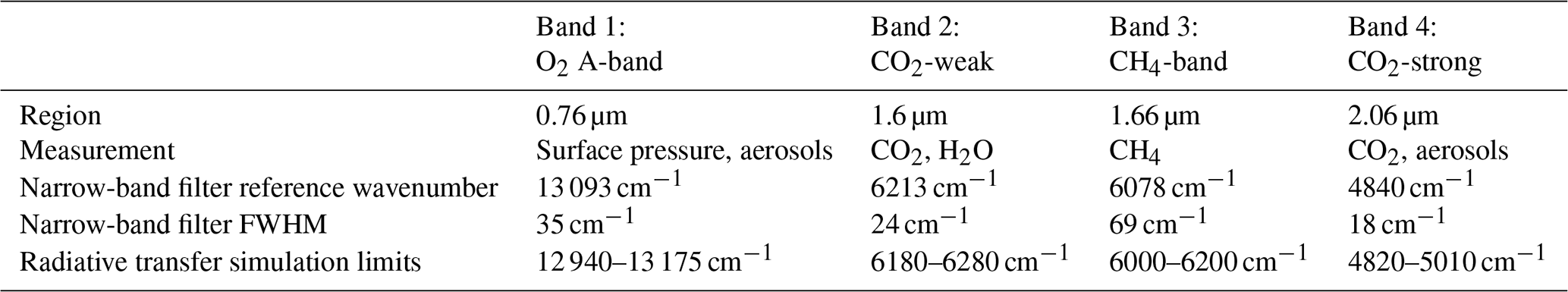
Figure 1 Example of a complete NanoCarb measurement. The left-hand panels show the measured intensities for the four spectral bands (denoted BD in the figure) for all their 60 OPDs and for all FOV pixels. The right-hand panel illustrates the FOV intensity for one given OPD. This example has been computed for a vegetation surface type, with a solar zenith angle of 25^∘.

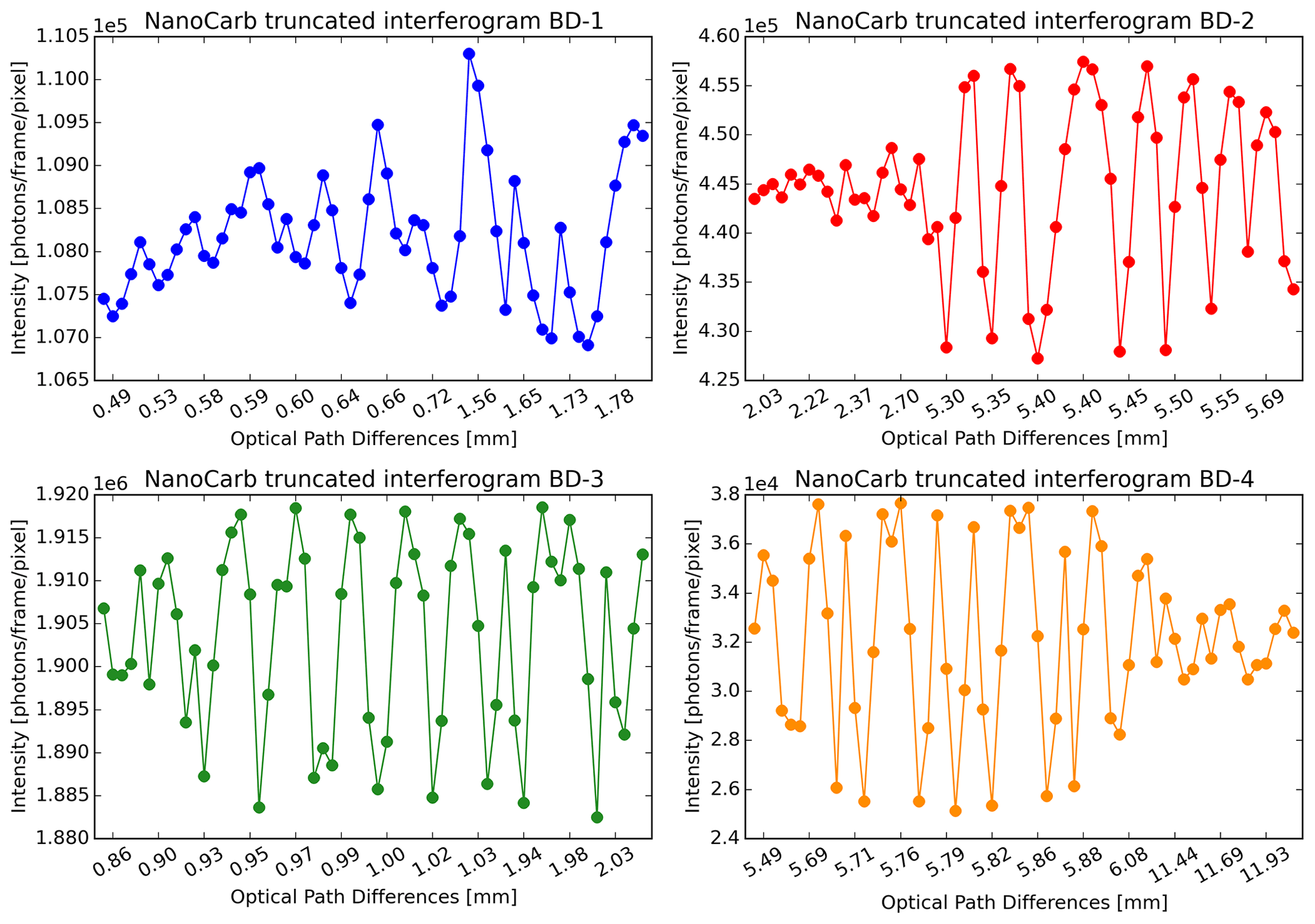
Figure 2 Example of a NanoCarb truncated interferogram for the four spectral bands (denoted BD in the figure), for a central pixel of the field of view, simulated for the same situation as for Fig. 1. Intensities are plotted as a function of the OPD indices as the OPD sampling is very discontinuous.

This work uses the latest design of the NanoCarb concept, based on an selection of 60 OPDs per spectral band, optimised for the central part of a FOV that accommodates 170 (across-track, θ_T between −9.3 and 9.3^∘) ×102 (along-track, θ_L between −5.5 and 5.5^∘) ground 1.15×1.15 km² pixels. This latest NanoCarb design hypothesis takes into account entanglements between CO₂, CH₄, O₂, H₂O and aerosols signals, with the assumption that albedo models are constant over all four spectral bands. As this study is the first L2 performance assessment for the NanoCarb concept, choices made for the state vector design (see Sect. 3.2) and simulation setups (see Sect. 4.2) are consistent with those hypotheses. Here, we use a NanoCarb instrumental model that implements (1) a model of the spectral transmission for a three-cavity narrow-band filter that simulates the angular dependency within the FOV and (2) an analytical approximation of the Fabry–Pérot transmission (Gousset et al., 2019). Given a synthetic radiance spectrum, computed by a line-by-line forward radiative transfer model, and the transversal θ_T and longitudinal θ_L angles characterising a given ground pixel within the FOV, it yields a NanoCarb truncated interferogram. This analytical model assumes perfect processing of the raw measurements and does not account for possible optical defects (such as stray light) or instrumental inaccuracies (such as faulty thermal regulation, which impact is assessed separately), nor does it take into account the point spread function (PSF) of the instrument.

2.2 SPEXone

SPEX (Spectro-Polarimeter for Planetary Exploration) is a family of aerosol sensors that have been co-developed by the Netherlands Institute for Space Research (SRON) and its academic and industrial partners. SPEXone, the latest and most compact multi-angle polarimeter of this family (6 dm³), is currently being developed by SRON, supported by optical expertise from Airbus Defence and Space Netherlands and the Netherlands Organisation for Applied Optics (TNO) (van Amerongen et al., 2019). It measures visible light at five viewing angles ±50, ±20 and 0^∘ along the satellite track and makes use of the spectral modulation technique (Snik et al., 2009) to encode the degree of linear polarisation (DoLP) in the measured spectrum. Radiance measurements will be provided at the spectral sampling (1 nm) and resolution (2 nm) of the spectrometer. The DoLP will be provided at 50 spectral bands with a spectral resolution ranging from about 10–30 nm. A key feature of SPEXone is that it is designed to measure the DoLP at very high accuracy (0.003, comprising both systematic and random errors) allowing the retrieval of aerosol size, refractive index, and single-scattering albedo in addition to the aerosol optical depth (AOD) (Hasekamp et al., 2019).

2.3 Sizing of the SCARBO constellation concept

The constellation sizing aims at ensuring intra-daily revisit of the largest possible amount of anthropogenic CO₂ emission hotspots. Those are defined as small areas which emission rate produce an $X_{{\mathrm{CO}}_{\mathrm{2}}}$ enhancement that can be detected with the 1 ppm SCARBO $X_{{\mathrm{CO}}_{\mathrm{2}}}$ precision objective. For this purpose, we use the reprocessing of the Open Source Data Inventory of Anthropogenic CO₂ (ODIAC) database compiled by Wang et al. (2019). They identified the emission clumps (area and point fossil fuel emission CO₂ sources) that are compatible with the detection of an $X_{{\mathrm{CO}}_{\mathrm{2}}}$ anthropogenic plume by a satellite flying around noon for different levels of $X_{{\mathrm{CO}}_{\mathrm{2}}}$ precision. Figure 3 shows the repartition of the emission hotspots compatible with the 1 ppm SCARBO precision objective and gives the revisit statistics over these hotspots for a constellation of 22, 24 or 26 satellites flying at 600 km on sun-synchronous orbits and equally distributed over two orbital planes at 10:00 and 14:00 local time (LT). With 24 satellites, the SCARBO constellation provides global coverage and guarantees daily revisit for all hotspots and intra-daily revisit for 73 % of the hotspots (those beyond ±30^∘ of latitude). This number of satellites provides an optimal compromise between coverage, cost, and available launch and deployment capabilities.

Figure 3 Map of hotspots (point sources in red, and other types of emission clumps in blue) with an emission rate compatible with the detectability of an $X_{{\mathrm{CO}}_{\mathrm{2}}}$ plume around noon with a 1 ppm precision spaceborne instrument. Yellow, green and blue horizontal lines give the minimum latitude for better intra-day revisit for a constellation of 22, 24 and 26 satellites, respectively. The left panel gives the corresponding average number of revisits as a function of latitude for a constellation of 22, 24 and 26 satellites, respectively.

3 Methodology

3.1 General approach

Level 4 atmospheric flux inversions targeting regional or global scales exploit extensive amounts of Level 2 products. The preparation of planned satellite missions usually includes observing system simulation experiments (OSSEs) that build a realistic numerical model of the atmosphere and simulate the instrument orbit and its measurements, upon which retrieval algorithms are then tested. This kind of computationally expensive approach is out of scope for the early stage readiness of the NanoCarb truncated interferogram concept. This is why we propose here to follow the approach used for CarbonSat preparation (Buchwitz et al., 2013).

First, given synthetic atmospheric and aerosol models (Sect. 4.1), we introduce five scattering-error-critical atmospheric and observational parameters (Sect. 4.2) for which we simulate synthetic NanoCarb truncated interferograms (without adding a random draw of artificial noise to them) for parameter values that span realistic intervals. Following this, for two different SCARBO design scenarios (without and with SPEXone, described in Sect. 4.3) we assess the L2 performance of the concept by performing inverse radiative transfer to retrieve $X_{{\mathrm{CO}}_{\mathrm{2}}}$ and $X_{{\mathrm{CH}}_{\mathrm{4}}}$ directly from the previously simulated synthetic NanoCarb measurements. Key L2 performance results presented in Sect. 5 comprise the systematic and random errors of the retrieved $X_{{\mathrm{CO}}_{\mathrm{2}}}$ and $X_{{\mathrm{CH}}_{\mathrm{4}}}$, as well as the vertical sensitivities of these retrieved columns, which are, for instance, essential to yield pseudo-observed columns from simulated GHG concentration profiles. Finally, those results are parameterised as functions of the selected scattering-error-critical atmospheric and observational parameters (Sect. 6). This yields fast and easily usable L2 performance models that enable the production of large amounts of L2 data.

3.2 Retrieval method: the 5AI inverse scheme

In the context of this work, inverse radiative transfer aims to determine the geophysical parameters and their uncertainties that best explain a given noised infrared measurement. For this purpose, we use the 5AI retrieval scheme (Dogniaux et al., 2021) that implements the optimal estimation (hereafter denoted OE) inverse method, iterating with a Levenberg–Marquardt optimisation method (Rodgers, 2000).

Table 2 5AI retrieval state vector.

In the framework of OE, we consider a state vector x, containing various geophysical variables that adequately describe the state of the atmosphere and of the surface, and a measurement vector y (here, the NanoCarb truncated interferogram). Both are Gaussian random variables described by an average and an uncertainty given in a covariance matrix. Prior to the measurement, climatologies or ad hoc choices describe the knowledge of the state x: this is called the a priori state. Its uncertainty has a strong impact on the retrieval result as it constrains how the measurement can be allowed to modify the state. Given this a priori state with its uncertainty and the measurement y, the uncertainty of which is known thanks to the noise characteristics of the instrument, OE enables us to find the most probable a posteriori state $\widehat{\mathit{x}}$ that best fits the measurement y, thus verifying the following equation:

$$\begin{array}{}\text{(1)}& \mathit{y}=\mathit{F}\left(\mathit{x}\right)+\mathit{\epsilon },\end{array}$$

with F being the forward radiative transfer model that describes the physics linking the state to the measurement and ε the measurement noise for which statistics are known from the instrument and detector characteristics. Besides, OE relies on a Bayesian formalism that translates the measurement uncertainty into state uncertainty, thus yielding an a posteriori covariance matrix for the retrieved a posteriori state $\widehat{\mathit{x}}$ that describes the estimation random error. Finally, OE also provides the averaging kernel matrix, usually denoted A, which describes how the retrieved state $\widehat{\mathit{x}}$ relates to the true (but unknown) values of its chosen parameters.

The key L2 performance results that we seek to determine are computed from these outputs: (1) the systematic errors of the retrieved $X_{{\mathrm{CO}}_{\mathrm{2}}}$ and $X_{{\mathrm{CH}}_{\mathrm{4}}}$ are defined as the differences between retrieved columns, computed from the a posteriori state $\widehat{\mathit{x}}$, and the synthetic true column; (2) $X_{{\mathrm{CO}}_{\mathrm{2}}}$ and $X_{{\mathrm{CH}}_{\mathrm{4}}}$ random errors are computed from the a posteriori covariance matrix; and (3) $X_{{\mathrm{CO}}_{\mathrm{2}}}$ and $X_{{\mathrm{CH}}_{\mathrm{4}}}$ vertical sensitivities are described by the column-averaging kernels, computed from the averaging kernel matrix A.

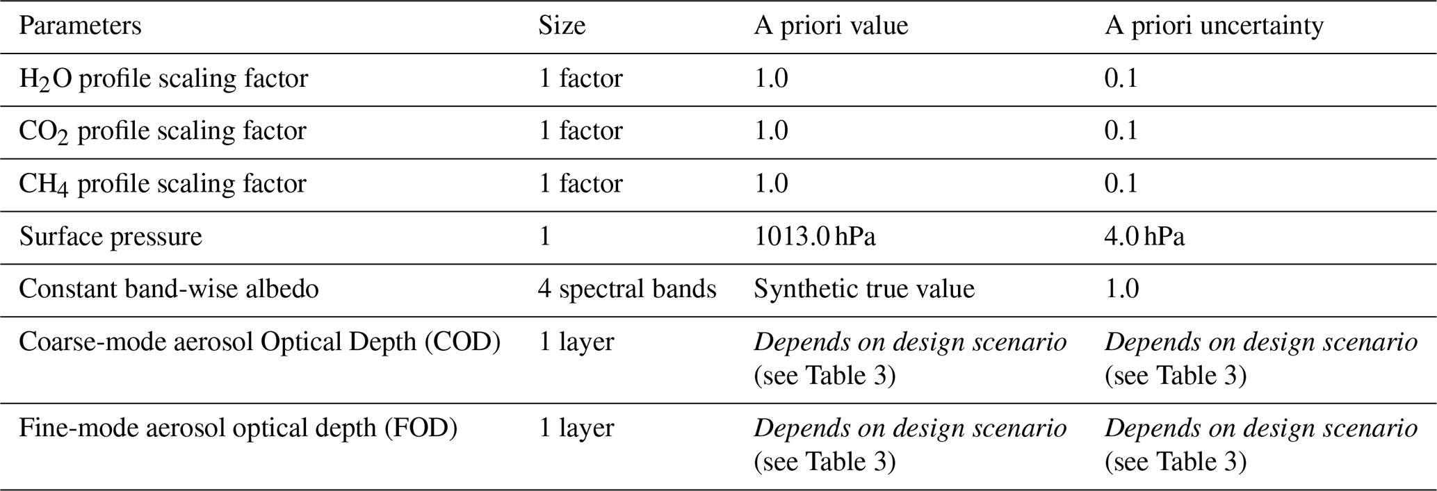
Here, 5AI state vector includes all the main geophysical variables that impact shortwave infrared radiative transfer and may interfere with $X_{{\mathrm{CO}}_{\mathrm{2}}}$ and $X_{{\mathrm{CH}}_{\mathrm{4}}}$ retrieval. Table 2 describes the state vector, the a priori value of its elements and their prior uncertainties (no covariance is taken into account). The interfering impact of atmospheric temperature has not been taken into account for the latest optimised OPD selection used in this work and is not considered in the state vector. In addition, except for the prior uncertainties of the aerosol optical depths, which depend on the design scenario we consider (see Sect. 4.3), all the prior uncertainties are purposefully large as we also aim to determine the information content of the NanoCarb truncated interferogram. Finally, the standard deviation of the instrument noise used for the 5AI retrievals can be calculated as follows:

$$\begin{array}{}\text{(2)}& {\mathit{\epsilon }}_{i,j}=\sqrt{I_{i,j}+r_j^{\mathrm{2}}},\end{array}$$

with ε_i,j being the standard deviation of the a priori noise for the ith OPD of the jth spectral band, I_i,j being the truncated interferogram intensity for the ith OPD of the jth spectral band, and r_j being the readout noise of the spectral band camera detector.

For its forward radiative transfer simulations, the 5AI scheme relies on the operational version of the Automatized Atmospheric Absorption Atlas (4A/OP) (Scott and Chédin, 1981) that is coupled with the Linearized Discrete Ordinate Radiative Transfer model (LIDORT, Spurr, 2002) in order to take into account multiple scattering caused by thin clouds and/or aerosols. Regarding spectroscopy, we use the 2015 version of the Gestion et Études des Informations Spectroscopiques Atmospheìriques: Management and Study of Atmospheric Spectroscopic Information (GEISA) spectroscopic database (Jacquinet-Husson et al., 2016), and we take into account line-mixing and collision-induced absorption in the O₂ A-band (Tran and Hartmann, 2008), as well as line-mixing and H₂O-broadening of CO₂ lines (Lamouroux et al., 2010).

For this work, in order to take into account the use of truncated interferograms, 5AI is coupled to the NanoCarb instrumental model: for all the spectral bands defined in Table 1, a synthetic spectrum and its partial derivatives with regard to the state variables (also called Jacobians) are computed line-by-line by 4A/OP and used as inputs to the NanoCarb instrumental model. It yields a NanoCarb truncated interferogram and its partial derivatives, which are the measurement and its Jacobians used within the 5AI scheme in this work, respectively. As an example, Fig. 4 shows the partial derivatives with regard to the 5AI state vector elements of the NanoCarb truncated interferogram shown in Fig. 2.

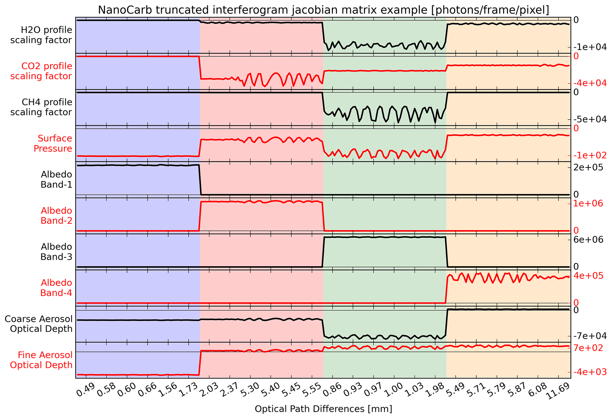
Figure 4 Example of a NanoCarb truncated interferogram Jacobian matrix for the 5AI state vector geophysical variables used in this work. It corresponds to the NanoCarb truncated interferogram shown in Fig. 2. Again, partial derivatives are plotted as a function of the OPD indices as the OPD sampling is very discontinuous.

3.3 Field of view

One NanoCarb measurement is not made of one truncated interferogram but of 170 (across-track) ×102 (along-track) truncated interferograms measured in snapshot mode in the instrument field of view. As the foreseen time between two consecutive snapshots corresponds to the FOV moving by one ground pixel, up to 102 independent single-pixel NanoCarb truncated interferograms can be measured for a given fixed location on the ground, during the ∼20 s overflight by the SCARBO satellite. The strategy to achieve precision below 1 ppm and 6 ppb for $X_{{\mathrm{CO}}_{\mathrm{2}}}$ and $X_{{\mathrm{CH}}_{\mathrm{4}}}$, respectively, is then to combine (for details, see Appendix A), for every ground pixel associated with a transversal position θ_T within the swath, all their respective available along-track single-pixel measurements in order to retrieve one final unique state of the atmosphere per transversal position. Consequently, all the NanoCarb retrieval results presented in this work also depend on the transversal position θ_T of the situation within the swath.

Several hypotheses are made to speed up calculations within the FOV. Because we assume that it is uniform, it suffices to compute single-pixel L2 results for the whole FOV and then combine them in the along-track direction in order to simulate the final L2 results. In addition, we assume that the along-track direction is aligned with the sun, and single-pixel L2 results are thus perfectly symmetrical with respect to the longitudinal axis (results can be shown for positive values of θ_T only) and nearly symmetrical (because of the impact of the asymmetrical aerosol phase function) with respect to the transversal axis. In reality, due to the very nature of NanoCarb measurements (see interference rings in Fig. 1), single-pixel L2 results exhibit a near-central symmetry. Processing all 170×102 pixels within the FOV would lead to unmanageable computation times, this is why we make use of the near-central symmetry in single-pixel L2 results to perform retrievals for a careful selection of 23 NanoCarb FOV pixels only (see the Supplement). Single-pixel L2 performance results are then interpolated from those 23 selected pixels to the whole FOV. Assuming that the CO₂ and CH₄ state vector parameters can be retrieved independently from the other geophysical variables, we then combine the single-pixel L2 performance results for $X_{{\mathrm{CO}}_{\mathrm{2}}}$ and $X_{{\mathrm{CH}}_{\mathrm{4}}}$ in the along-track direction following (for scalar quantities) the method described in Appendix A. This last step yields final L2 performance results that only depend on the transversal position θ_T within the swath, in addition to the five atmospheric and observational parameters considered here (see Sect. 4). Errors arising from the interpolation have been assessed and are negligible (not shown, up to 0.01 ppm for $X_{{\mathrm{CO}}_{\mathrm{2}}}$ systematic and random errors and up to 0.05 ppb for $X_{{\mathrm{CH}}_{\mathrm{4}}}$ systematic and random errors, all evaluated on a test case). These final L2 results are, like single-pixel L2 results, symmetrical along θ_T, and thus only results for θ_T between 0 and 9.3^∘ need to be shown.

4 Simulation setups

4.1 Synthetic atmospheric and aerosol models

The L2 performance assessment presented here is done for an atmospheric situation representative of the meteorological conditions that can be found over Europe. More precisely, for all our inverse radiative transfer simulations, we use the average mid-latitude temperate atmospheric situation computed from the Thermodynamic Initial Guess Retrieval (TIGR) climatology library (Chedin et al., 1985) (available at https://ara.lmd.polytechnique.fr/index.php?page=tigr, last access: 9 August 2022). The corresponding temperature, water vapour and ozone profiles have been discretised over 20 pressure levels bounding 19 layers, as for the ACOS algorithm (O'Dell et al., 2018). The surface pressure is set to 1013 hPa. For this synthetic performance study, constant trace gas concentration profiles have been used: 394.85 ppm for CO₂ and 1855.3 ppb for CH₄. The use of these constant background GHG concentration profiles is a strong hypothesis, which is in line with the one chosen by Bovensmann et al. (2010) for CarbonSat performance studies. Eventually, realistic CO₂ and CH₄ profiles should be considered in full OSSEs, as the SCARBO concept improves in its readiness.

We consider the presence of two aerosol modes in the atmosphere: a fine mode and a coarse mode. This assumption is in line with the ones made for the SPEXone retrieval capability study (Hasekamp et al., 2019) and, apart from the cirrus contribution, follows the assumptions made for the full physics retrieval algorithm developed at the University of Leicester (Cogan et al., 2012). Here, the fine aerosol mode is treated under a log-normal size distribution with an effective size of 0.20 µm, an effective variance of 0.2 µm and a refractive index of $\mathrm{1.50}+{\mathrm{10}}^{-\mathrm{7}}i$. This fine mode is representative of typical industrial non-organic aerosols and is located in a fixed atmospheric layer between 0 and 2 km. As for the coarse mode, it is treated under a log-normal size distribution with an effective size of 1.6 µm, an effective variance of 0.6 µm, a refractive index of 1.53+0.00254i and a spheroid fraction of 0.95. This coarse mode is representative of typical mineral dust and is located at a varying altitude. Non-spherical aerosols are described as a size–shape mixture of randomly oriented spheroids, and we use the Mie- and T-matrix-improved geometrical optics database by Dubovik et al. (2006) along with their proposed spheroid aspect ratio distribution for computing optical properties (extinction coefficient, single-scattering albedo and asymmetry parameter) for a mixture of spheroids and spheres. These optical properties are then used as inputs to the 5AI scheme.

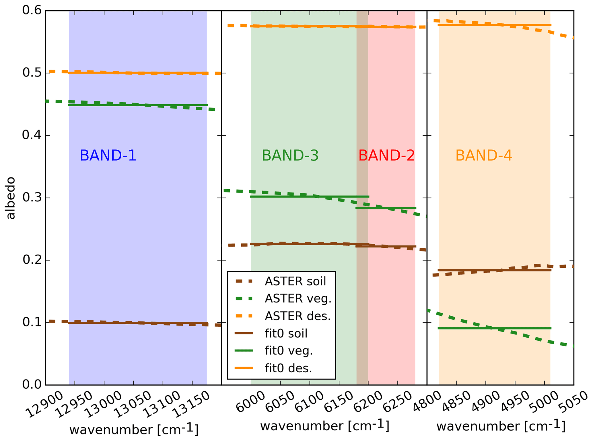
Figure 5 True spectral dependence of the three albedo models considered in this work. Constant band-wise fits of these models are used here.

Table 3 Summary of no-SPEX and with-SPEX design scenario assumptions.

4.2 Atmospheric and observational parameters for L2 performance assessment

We consider five parameters related to scattering error: (1) the albedo model, (2) the solar zenith angle, (3) the coarse layer height, (4) the coarse-mode aerosol optical depth, and (5) the fine-mode aerosol optical depth. Those are usual parameters considered for L2 performance assessments as they can strongly impact the photon optical path or the overall amount of signal measured by the satellite detector (Boesch et al., 2011; Buchwitz et al., 2013). Different values for these five parameters are explored, yielding a set of 324 atmospheric and observational situations for which the SCARBO L2 performance assessment is performed.

Regarding albedo (hereafter ALB), we consider three different ground albedo models representative of soil, vegetation and desert scenes that are generated from the ASTER spectral library (Baldridge et al., 2009). As detailed in Sect. 2, the current optimisation of the NanoCarb OPDs assumes constant band-wise albedos. Hence, in this work, the simulated NanoCarb truncated interferograms and the $X_{{\mathrm{CO}}_{\mathrm{2}}}$ and $X_{{\mathrm{CH}}_{\mathrm{4}}}$ retrievals use the same assumption: Fig. 5 shows the spectral dependence of the three albedo models we consider, as well as the constant band-wise fits used for all simulations.

For solar zenith angle (SZA), we explore four different values: 0, 25, 50, and 70^∘. Though shortwave infrared soundings can be made at higher SZAs, experience from OCO-2 post-filtering by the ACOS algorithm shows that soundings at high SZAs are more often removed (O'Dell et al., 2018), thus studying a maximum SZA of 70^∘ is a reasonable compromise.

Concerning coarse aerosol mode layer height (CLH), we assume possible altitudes of 2, 4 and 6 km and coarse aerosol mode optical depths (CODs) explore the following values: 0.001, 0.05 and 0.15 at 550 nm reference wavelength. Fine aerosol mode optical depths (FODs) explore 0.001, 0.12, 0.22 at 550 nm reference wavelength. The aerosol synthetic setup proposed here aims to represent (1) background aerosol optical depth, arbitrarily attributed to industrial non-organic aerosols (as those are expected around and downwind of strong emission hotspots) with optical depth values consistent for instance with MODIS observed averages over Europe for 2010 (Palacios-Peña et al., 2019) and (2) transient coarse mineral desert dust layers that can be observed over Europe in late spring, summer and early autumn with a varying altitude (Papayannis et al., 2008).

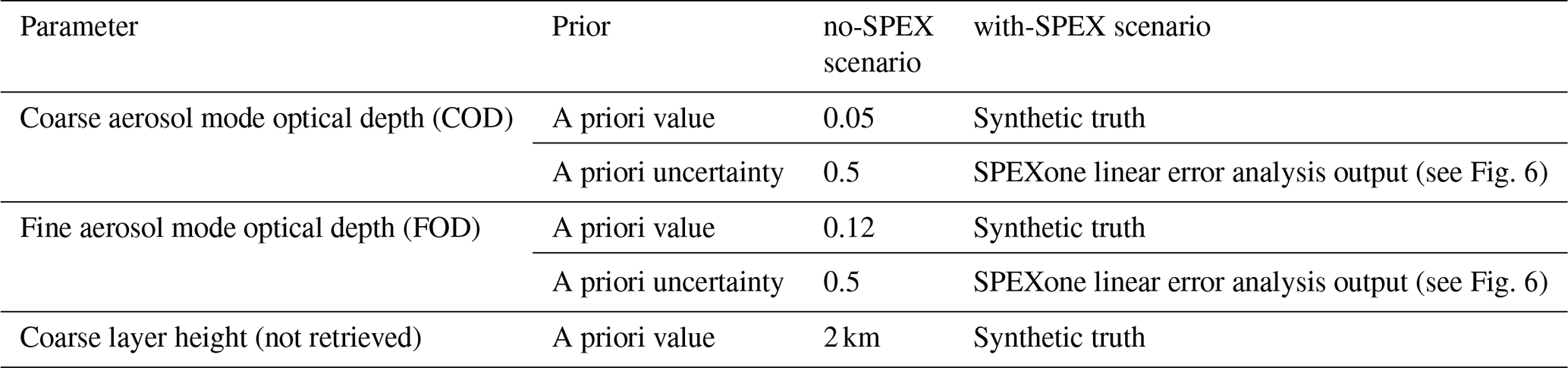
4.3 Two design scenarios: without and with SPEXone

Two SCARBO satellite design scenarios are studied in this work. Table 3 summarises the assumptions made for both scenarios: they are only related to the a priori setups of 5AI NanoCarb retrievals.

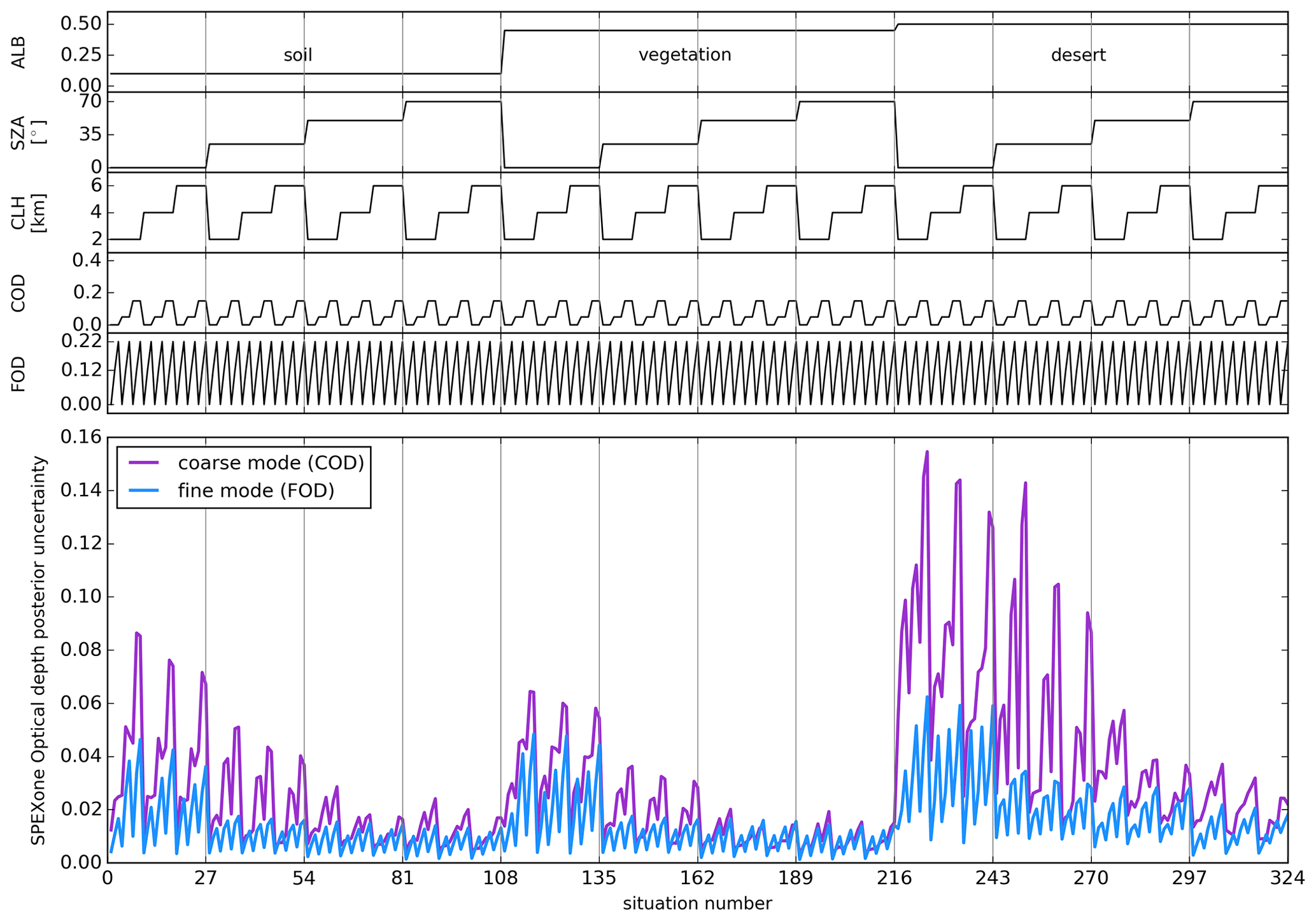
Figure 6 SPEXone linear error analysis results for all the 324 atmospheric and observational situations used in this work. SPEXone COD and FOD posterior uncertainties are plotted against the situation number: the top five panels detail the ALB (0.7 µm), SZA, CLH, COD and FOD values defining all 324 situations.

The first one, hereafter referred as “no-SPEX”, simulates a SCARBO satellite only carrying the NanoCarb instrument. This scenario is simulated with fixed a priori values for COD and FOD in the state vector and with a fixed CLH of 2 km, regardless of the atmospheric and observational situation considered. The random prior uncertainties for COD and FOD are set to 0.5, a large value also reflecting the limited knowledge of aerosol parameters in this design scenario.

The second design scenario, hereafter referred as “with-SPEX”, simulates a SCARBO platform carrying both SPEXone and NanoCarb instruments at the same time, thus yielding co-located SPEXone and NanoCarb measurements. For this scenario, we consider a two-step L2 retrieval approach in which SPEXone measurements are analysed first. These results are then used to improve the a priori constraints on aerosol parameters in second-step GHG column retrievals from NanoCarb measurements. The first step is fulfilled by a linear error analysis that yields SPEXone posterior uncertainties for COD and FOD, following the method described in Hasekamp et al. (2019). Figure 6 shows these SPEXone random errors for the coarse-mode (COD) and fine-mode (FOD) aerosol optical depths for all the 324 atmospheric and observational situations considered in this work. Its first five top panels have a descriptive purpose: they recall the values of the ALB, SZA, CLH, COD and FOD parameters for all 324 situations. Thus, the first third of the x axis is dedicated to soil albedo situations, the second third is dedicated to vegetation albedo situations, and the final third is dedicated to desert albedo situations. For all of these ALB cases, all SZA values are explored, as are all scattering particle cases for all ALB cases and SZA values, thus sorting all of the 324 considered situations along one dimension (an identical sorting is used in Figs. 7, 9, 10, and 11). Regarding SPEXone performance, the posterior uncertainties in optical depth are correlated to the optical depth values and are lower for the fine mode compared to the coarse mode. Uncertainties are higher for desert albedo situations as the ratio between scattered photons and surface-reflected photons is lower over desert compared to soil or vegetation situations. For both modes they improve with increasing SZA values because the light path through the aerosol layer increases but also because a wider scattering angle range, that is also closer to 90^∘, is typically encountered at higher SZA (Hasekamp et al., 2019; Fougnie et al., 2020). Posterior uncertainties of coarse-mode optical depths are also decreasing with CLH values as more photons are scattered when the coarse layer height increases. For the with-SPEX design scenario considered here, these COD and FOD posterior uncertainties are used as a priori uncertainties within the second-step GHG column retrievals from NanoCarb measurements. In addition, in the absence of full SPEXone retrieval results, we also assume that the first-step SPEXone measurement analyses yield perfectly accurate COD and FOD values, as well as the true synthetic CLH values (aerosol layer heights are not retrieved from NanoCarb measurements, as per Table 2, but can be obtained from SPEXone retrievals).

5 Results and discussion

5.1 Geophysical information content and variable entanglements in NanoCarb truncated interferograms

In this work, $X_{{\mathrm{CO}}_{\mathrm{2}}}$ and $X_{{\mathrm{CH}}_{\mathrm{4}}}$ are directly retrieved from truncated interferograms sampled at OPDs optimally sensitive to CO₂, CH₄ and possibly interfering geophysical variables. This peculiar nature of NanoCarb measurements strongly differs from usual infrared spectra (measured for example by GOSAT or OCO instruments). A way to evaluate the geophysical information content is to examine the optimal estimation degrees of freedom (hereafter denoted “DOFs”) that provide, for all state vector variables, the amount of useful independent quantities provided by the measurement, whatever its nature (Rodgers, 2000).

Figure 7 shows NanoCarb state vector DOFs, averaged over the 23 selected FOV pixels, for all 324 atmospheric and observational situations considered in this work (described in the top five panels, as in Fig. 6), as well as for both no-SPEX and with-SPEX design scenarios. Grey-shaded areas in the no-SPEX design scenario case remove situations for which the retrievals did not satisfactorily converge. Overall, we can notice that CO₂ and CH₄ DOFs are close to 1.0, confirming the sensitivity of the retrievals and of NanoCarb measurements to these two target greenhouse gases. In the no-SPEX design scenario, COD DOFs have similar values, thus underlying a significant sensitivity of NanoCarb measurement to the coarse-mode aerosol layer. All albedo bands have near 1.0 DOFs, and for other variables, comprising water vapour profile scaling factor, surface pressure and FOD, retrievals do not get much information from NanoCarb measurements. This means that the retrievals rely on their a priori information for these variables, which can result in systematic $X_{{\mathrm{CO}}_{\mathrm{2}}}$ and $X_{{\mathrm{CH}}_{\mathrm{4}}}$ biases if the a priori data are biased compared to the true state of the atmosphere. For the no-SPEX design scenario case, the DOF evolution is mainly explained by the strong sensitivity of NanoCarb measurements to COD. This COD sensitivity increases for situations with SZA =70^∘ because spaceborne measurements are more sensitive to scattering for highly slanted optical paths. Conversely, this explains the drop in the other variable DOFs for which less measurement information is available in situations with SZA =70^∘. For all geophysical variables but albedo and surface pressure, the variations of DOFs are correlated with COD: the large 0.5 a priori uncertainty for COD in no-SPEX retrievals brings only a mild constraint that results in the COD parameter driving the information content for all the other variables.

Figure 7 NanoCarb state vector variable degrees of freedom averaged over the 23 FOV pixels used to interpolate L2 results to the whole FOV. Results are plotted as a function of the situation number: the top five panels detail the ALB (0.7 µm), SZA, CLH, COD and FOD values defining all 324 situations. Grey-shaded areas denote situations for which retrievals did not satisfactorily converge.

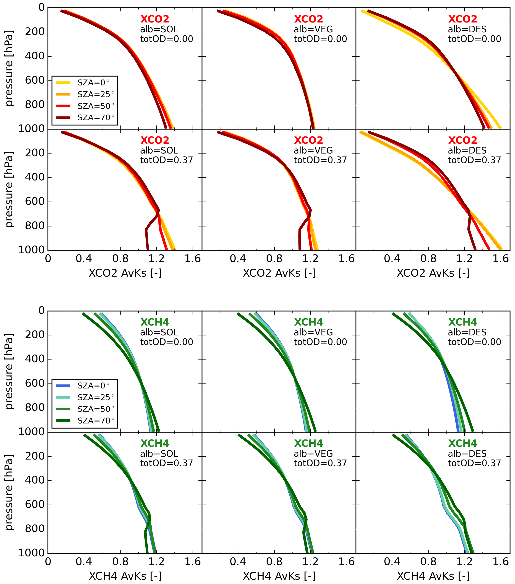
Figure 8 NanoCarb $X_{{\mathrm{CO}}_{\mathrm{2}}}$ (top panels) and $X_{{\mathrm{CH}}_{\mathrm{4}}}$ (bottom panels) column-averaging kernels averaged over the 23 FOV pixels used to interpolate L2 results to the whole FOV. We show all three albedo models, soil (left), vegetation (middle), and desert (right), and four different SZA values (colour scales). Averaging kernels are shown for a low total aerosol optical depth (top rows) and a high total aerosol optical depth (bottom rows).

The with-SPEX design scenario exhibits much reduced aerosol parameter DOFs arising from NanoCarb interferograms: this scenario is designed so that SPEXone, with improved a priori constraints in GHG retrievals, brings much of the information regarding aerosol parameters. Consistent with the SPEXone performance shown in Fig. 6, FOD DOFs are nearly equal to 0 thanks to SPEXone performance and the NanoCarb measurements' mild sensitivity to fine-mode aerosols. As for coarse-mode aerosols, the remaining COD DOFs are the result of the strong sensitivity of NanoCarb measurements to this mode and of SPEXone' lower performance for coarse mode: with-SPEX COD, DOFs are well correlated with the SPEX posterior uncertainties for COD shown in Fig. 6. One can also note that, when viewing the similar SPEXone performance between fine and coarse modes at high SZAs in soil and vegetation cases, COD DOFs are much larger than FOD DOFs, once again underlining the sensitivity of NanoCarb measurements to the coarse mode. For low SZAs in desert albedo situations, where SPEXone performance for coarse mode is at its lowest and has large remaining uncertainties, COD DOFs are high, meaning that NanoCarb measurements can contribute to constraining coarse-mode aerosols in these situations. Symmetrically to reducing the amount of NanoCarb measurement information used to constrain aerosol parameters, the use of SPEXone posterior results in NanoCarb GHG retrievals helps by using more of this information to constrain other variables. Consequently, GHG, surface pressure and albedo DOFs increase in the with-SPEX (with regard to no-SPEX) scenario, as shown in Fig. 7 (the increase is very small and not distinguishable for albedo). This underlines the geophysical information entanglement of the latter variables with aerosol parameters in NanoCarb measurements.

Retrieving a profile scaling factor for CO₂ or CH₄ instead of a layered profile has the advantage of setting a 1.0 limit to the DOFs these gases can have. Given the state vector used in this work, reaching this 1.0 DOF limit value for all geophysical variables would mean that all of them could be retrieved independently of each other. Failing to do so as shown in Fig. 7 for the with-SPEX scenario means that the geophysical information is entangled in NanoCarb measurements: variables cannot be retrieved independently of each other and correlations exist. A way to identify main variable-to-variable entanglements is to examine similarities (correlation or anticorrelations) between the partial derivatives of state vector elements. For example, Fig. 4 displays a correlation between albedo and CO₂ Jacobians in NanoCarb band 2: both evolve similarly around different continuous components. Though less visible or not visible due to scale, similar similarities exist between surface pressure and albedo Jacobians in band 1 (anticorrelation), the CH₄ profile scaling factor and H₂O or albedo Jacobians in band 3 (correlations), and the CO₂ profile scaling factor and albedo Jacobians in band 4 (anticorrelation). Thus CO₂, albedo and aerosol variables are entangled in the current OPD optimisation of NanoCarb measurement, and the same is true for CH₄ information, which is also entangled with H₂O.

5.2 Vertical sensitivities: column-averaging kernels

Column-averaging kernels (hereafter referred as “AKs”) describe the vertical sensitivity of retrieved $X_{{\mathrm{CO}}_{\mathrm{2}}}$ and $X_{{\mathrm{CH}}_{\mathrm{4}}}$. In other words, they show which atmospheric layers contribute the most to the GHG information contained in the measurement. NIR and SWIR spectrum measurements are typically sensitive to the whole atmospheric column, with AKs that reach their maximum in atmospheric layers close to the surface and then decrease with altitude above the mid-troposphere (e.g. for OCO-2, see Boesch et al., 2011). Figure 8 presents the NanoCarb $X_{{\mathrm{CO}}_{\mathrm{2}}}$ and $X_{{\mathrm{CH}}_{\mathrm{4}}}$ AKs for all albedo models and SZAs and for the minimum and maximum total aerosol optical depth (AOD) situations. As for usual NIR and SWIR concepts such as OCO-2 or S5-P/TROPOMI, NanoCarb truncated interferograms are sensitive to CO₂ and CH₄ in all atmospheric layers. In addition, it can be noticed that NanoCarb AKs with low total AOD satisfactorily compare with those obtained for trace gas profile scaling factors retrieved from SCIAMACHY low-resolution measurements by the WFM-DOAS algorithm (Bovensmann et al., 1999; Buchwitz et al., 2005). Indeed, like WFM-DOAS $X_{{\mathrm{CO}}_{\mathrm{2}}}$ AKs, NanoCarb $X_{{\mathrm{CO}}_{\mathrm{2}}}$ AKs grossly evolve from 1.2–1.5 in the boundary layer to only 0.1–0.2 at the top of the atmosphere (TOA), and the same comparison stands for $X_{{\mathrm{CH}}_{\mathrm{4}}}$ AKs: both evolve from approximately 1.2 in the boundary layer to about 0.5 at TOA. SZA dependence of AKs appears to be quite similar between NanoCarb and SCIAMACHY or WFM-DOAS for $X_{{\mathrm{CH}}_{\mathrm{4}}}$ but is different for $X_{{\mathrm{CO}}_{\mathrm{2}}}$ AKs: sensitivity in the boundary layer and lower troposphere decreases with SZA in the NanoCarb case, whereas it increases for WFM-DOAS. Regarding NanoCarb AKs for atmospheric situations with the maximum aerosol optical depth, we can notice a sensitivity drop in the atmospheric layers containing aerosols for $X_{{\mathrm{CO}}_{\mathrm{2}}}$ AKs, especially at high SZAs. Even if comparing AKs shapes remain difficult because a CO₂ profile is retrieved (and not a scaling factor) and many other factors differ, a similar behaviour was noticed during the ACOS algorithm characterisation (Boesch et al., 2011). As for NanoCarb $X_{{\mathrm{CH}}_{\mathrm{4}}}$ AKs, they exhibit a slight increase of sensitivity in the atmospheric layers containing aerosols and a sensitivity drop comparable to NanoCarb $X_{{\mathrm{CO}}_{\mathrm{2}}}$ AKs for SZA =70^∘. No similar $X_{{\mathrm{CH}}_{\mathrm{4}}}$ AK sensitivity study for the presence of aerosol has been found when writing this article.

5.3 Systematic and random errors

The NanoCarb spectral band narrow-band filters exhibit FOV-dependent effects that impact the L2 performance: their reference wavelengths shift towards slightly shorter wavelengths with the angle of incident light, and thus with the distance of pixels to the centre of the FOV (Smith, 2008). As the OPD selection was optimised for the centre of the FOV, this results in an increased GHG and albedo information entanglement close to the swath border (not shown). This leads to an increase in $X_{{\mathrm{CO}}_{\mathrm{2}}}$ and $X_{{\mathrm{CH}}_{\mathrm{4}}}$ random errors, which can become slightly larger than the SCARBO precision objectives of 1 ppm and 6 ppb for few situations and FOV pixels. In addition, it also challenges the hypothesis of independent scalar columns that is used to combine the FOV single-pixel $X_{{\mathrm{CO}}_{\mathrm{2}}}$ and $X_{{\mathrm{CH}}_{\mathrm{4}}}$ results in the along-track direction. As a consequence, we choose here to only consider pixels with θ_T between −6 and 6^∘ (whereas the full swath spans ±9.3^∘ in the currently considered design used for constellation sizing).

Figure 9 shows, for all 324 atmospheric and observational situations and for all transversal angle positions between 0 and 6^∘, NanoCarb systematic and random errors (definitions are given in Sect. 3.2) for $X_{{\mathrm{CO}}_{\mathrm{2}}}$ and $X_{{\mathrm{CH}}_{\mathrm{4}}}$ in the no-SPEX design scenario case. As for Fig. 6, the five top panels describe ALB, SZA, CLH, COD and FOD values for all situations. A priori and retrieved values are also shown for COD and FOD in order to explain where $X_{{\mathrm{CO}}_{\mathrm{2}}}$ and $X_{{\mathrm{CH}}_{\mathrm{4}}}$ systematic errors come from. The four bottom panels display $X_{{\mathrm{CO}}_{\mathrm{2}}}$ and $X_{{\mathrm{CH}}_{\mathrm{4}}}$ systematic and random errors. Retrievals converge and satisfactorily reduce the cost function for most of the situations. Still, some of them remain challenging depending on the albedo model and SZA, when COD or CLH are far from the a priori value. Their results are excluded, as shown with the grey-shaded areas.

Figure 9 NanoCarb systematic and random errors for $X_{{\mathrm{CO}}_{\mathrm{2}}}$ and $X_{{\mathrm{CH}}_{\mathrm{4}}}$ in the no-SPEX design scenario case. Results are plotted as a function of the situation number: the five top panels detail the ALB (0.7 µm), SZA, CLH, COD and FOD values defining all 324 situations. In addition, the a priori and averaged retrieved COD and FOD values are also shown in the fourth and fifth top panels. The sixth and seventh panels show $X_{{\mathrm{CO}}_{\mathrm{2}}}$ systematic and random errors, respectively, and the eighth and ninth panels show $X_{{\mathrm{CH}}_{\mathrm{4}}}$ systematic and random errors, respectively. The dependence on the transversal angle θ_T of L2 results is shown with the colour scales: darker colours correspond to lower θ_T absolute values. Grey-shaded areas denote situations for which retrievals did not satisfactorily converge.

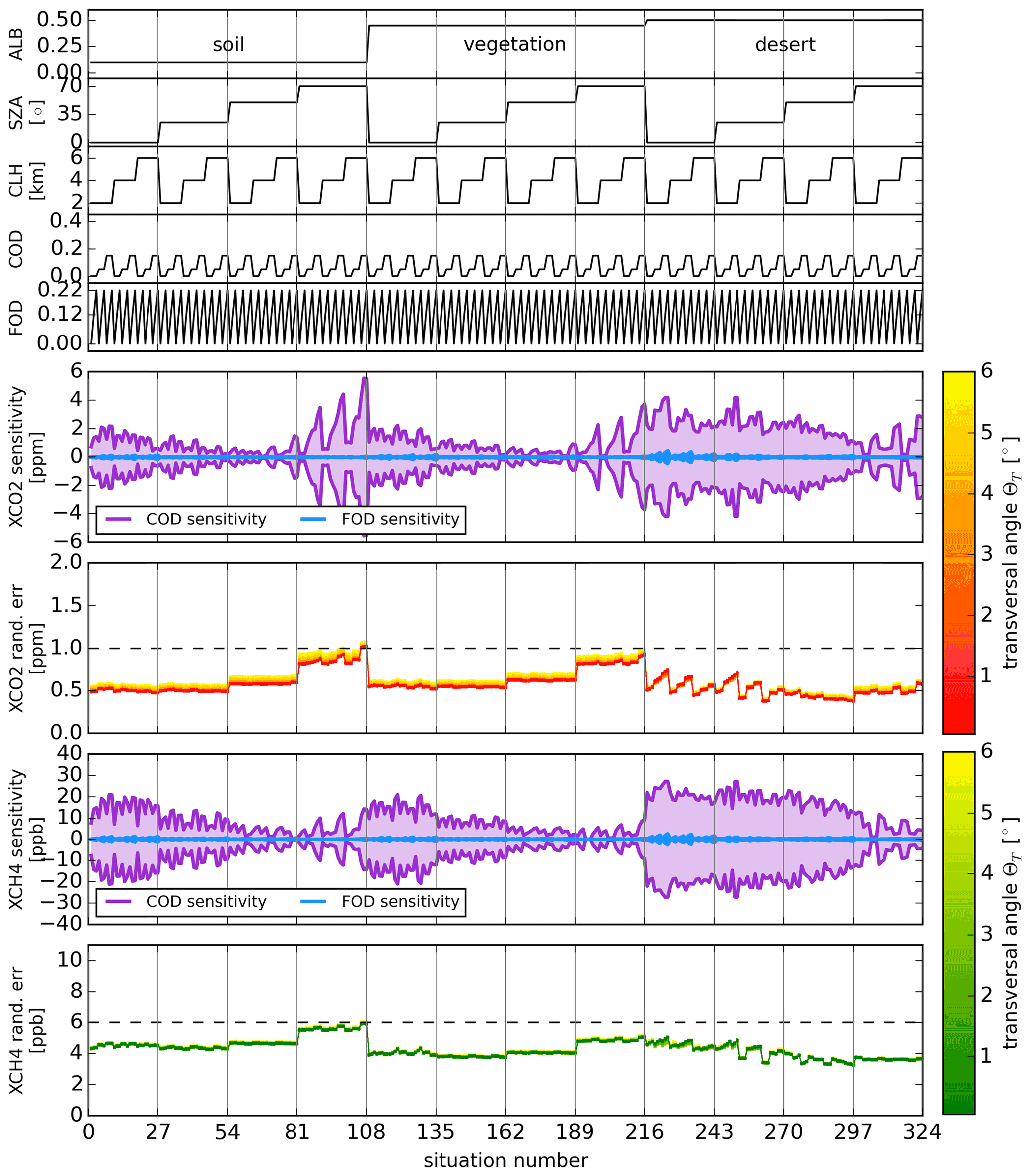
Figure 10 NanoCarb sensitivities to a priori misknowledge of COD and FOD and random errors for $X_{{\mathrm{CO}}_{\mathrm{2}}}$ and $X_{{\mathrm{CH}}_{\mathrm{4}}}$ in the with-SPEX design scenario case. Results are plotted as a function of the situation number: the five top panels detail the ALB (0.7 µm), SZA, CLH, COD and FOD values defining all 324 situations. The sixth and seventh panels show $X_{{\mathrm{CO}}_{\mathrm{2}}}$ sensitivities to a priori misknowledge of COD and FOD and random errors, respectively, and the eighth and ninth panels show $X_{{\mathrm{CH}}_{\mathrm{4}}}$ sensitivities to a priori misknowledge of COD and FOD and random errors, respectively. The dependence on the transversal angle θ_T of random errors results is shown with the colour scales: darker colours correspond to lower θ_T absolute values. As for sensitivities, only the minimum and maximum values for all transversal angles are shown.

In this no-SPEX case, systematic errors come from the erroneous prior knowledge of scattering parameters in the state vector (Fig. 9). Regarding scattering particles, NanoCarb measurements are mostly sensitive to the presence of coarse-mode aerosols in the optical path (as explained in Sect. 5.1), and the COD can be retrieved to some extent when the synthetic truth is not too far from the a priori state. Retrieved FOD seldom differ from the a priori value, showing again that no-SPEX retrievals are not very sensitive to fine-mode aerosols. Here, $X_{{\mathrm{CO}}_{\mathrm{2}}}$ and $X_{{\mathrm{CH}}_{\mathrm{4}}}$ systematic errors can reach up to 8 ppm and 30 ppb in absolute value for $X_{{\mathrm{CO}}_{\mathrm{2}}}$ and $X_{{\mathrm{CH}}_{\mathrm{4}}}$, respectively. This corresponds to about 10 times and 5 times their average random error, respectively. Thus, no-SPEX NanoCarb $X_{{\mathrm{CO}}_{\mathrm{2}}}$ retrievals are more sensitive to scattering error than no-SPEX NanoCarb $X_{{\mathrm{CH}}_{\mathrm{4}}}$ retrievals. $X_{{\mathrm{CO}}_{\mathrm{2}}}$ systematic errors are mostly driven by COD retrieval errors that correlate with CLH a priori misknowledge (CLH a priori value is here fixed at 2 km, see Table 3) and SZA. This SZA dependence of systematic errors is particularly important for $X_{{\mathrm{CO}}_{\mathrm{2}}}$; this may be explained by the use of the 2.05 µm CO₂ strong band, which includes saturated CO₂ lines and is quite sensitive to aerosols. A similar COD retrieval error dependence is found for $X_{{\mathrm{CH}}_{\mathrm{4}}}$ systematic errors, which also interestingly exhibit a stronger correlation to FOD retrieval error that is particularly visible in vegetation and desert albedo situations. $X_{{\mathrm{CO}}_{\mathrm{2}}}$ and $X_{{\mathrm{CH}}_{\mathrm{4}}}$ systematic error swath dependence are shown by the colour scales. It is most visible when systematic $X_{{\mathrm{CO}}_{\mathrm{2}}}$ errors are high at the swath centre, and in situations with COD values far from the a priori for $X_{{\mathrm{CH}}_{\mathrm{4}}}$.

Random errors in the no-SPEX design scenario (Fig. 9) for transversal positions below 6^∘ in absolute value outperform the 1 ppm SCARBO $X_{{\mathrm{CO}}_{\mathrm{2}}}$ precision objective for SZA below 50^∘ in soil and vegetation situations and for all SZA values in desert albedo situations. Regarding $X_{{\mathrm{CH}}_{\mathrm{4}}}$ random errors, they overall meet the 6 ppb precision objective but for soil albedo situations with SZA values of 25^∘ or lower. Within the OE formalism, random error variations are by definition completely correlated with DOFs variations (see Fig. 6), meaning that when more information is available for a given variable, its random error diminishes. Thus, as for DOFs, random error variations are mostly driven by COD and ALB values in the no-SPEX design scenario. It can finally be noted that most of the transversal positions within the swath exhibit similar random errors, except for those close to 6^∘.

As detailed in Table 3, the a priori aerosol profile and a priori state vector are identical to the true state of the synthetic atmosphere in the with-SPEX design scenario case. This is done to simulate a more precise and accurate knowledge of aerosol parameters that can be brought by the SPEXone instrument. Given this strong hypothesis for SPEXone retrieval accuracy, L2 retrieval results do not exhibit systematic errors. Consequently, in order to study the sensitivity of $X_{{\mathrm{CO}}_{\mathrm{2}}}$ and $X_{{\mathrm{CH}}_{\mathrm{4}}}$ systematic errors to this hypothesis, we use the averaging kernel matrix A to propagate a priori misknowledge of aerosol parameters. Following Rodgers' (2000) notations, we have

$$\begin{array}{}\text{(3)}& \mathrm{d}\widehat{\mathit{x}}={\displaystyle \frac{\partial \widehat{\mathit{x}}}{\partial {\mathit{x}}_{\mathrm{true}}}}\mathrm{d}{\mathit{x}}_{\mathrm{true}}=\mathbf{A}{\left[\mathrm{0},\mathrm{0},\mathrm{0},\mathrm{0},\mathrm{0},\mathrm{0},\mathrm{0},\mathrm{0},{\mathit{\delta }}_{\mathrm{COD}},{\mathit{\delta }}_{\mathrm{FOD}}\right]}^{\mathrm{T}},\end{array}$$

with $\widehat{\mathit{x}}$ being the retrieved state vector, x_true being the synthetic true state of the atmosphere, and δ_COD and δ_FOD being the differential perturbation of COD and FOD parameters, respectively.

Figure 10 is similar to Fig. 9, but shows results for the with-SPEX design scenario (a version that combines Figs. 9 and 10 is included in the Supplement for a better comparison of systematic errors but less readability of no-SPEX results). Instead of systematic errors, it presents $X_{{\mathrm{CO}}_{\mathrm{2}}}$ and $X_{{\mathrm{CH}}_{\mathrm{4}}}$ systematic error sensitivities to synthetic truth perturbations of COD and FOD corresponding to their respective prior uncertainties σ_COD and σ_FOD: ${\mathit{\delta }}_{\mathrm{COD}}=\pm {\mathit{\sigma }}_{\mathrm{COD}}$ and ${\mathit{\delta }}_{\mathrm{FOD}}=\pm {\mathit{\sigma }}_{\mathrm{FOD}}$ (provided by SPEXone linear error analysis). This systematic error sensitivity test is conservative in different ways. First, the perturbation by SPEXone random error is at least a factor of 2 greater than the systematic optical depth errors found in Hasekamp et al. (2019). In addition, the separation between COD and FOD perturbations does not allow for these errors to compensate themselves and possibly partially cancel out a fraction of $X_{{\mathrm{CO}}_{\mathrm{2}}}$ and $X_{{\mathrm{CH}}_{\mathrm{4}}}$ systematic errors. $X_{{\mathrm{CO}}_{\mathrm{2}}}$ and $X_{{\mathrm{CH}}_{\mathrm{4}}}$ systematic error sensitivities to synthetic truth perturbations of COD and FOD are shown as the maximum and minimum sensitivities among all transversal positions with $\mathrm{|}{\mathit{\theta }}_{\mathrm{T}}\mathrm{|}<\mathrm{6}{}^{\circ }$. Uncertainties in COD retrieved by SPEXone can result in up to ±5.5 ppm impact on $X_{{\mathrm{CO}}_{\mathrm{2}}}$ and ±28 ppb impact on $X_{{\mathrm{CH}}_{\mathrm{4}}}$. It is interesting to note that despite similar SPEXone precisions for COD and FOD between SZA =50^∘ and SZA =70^∘ over all albedo models, COD perturbations have a much more important impact on $X_{{\mathrm{CO}}_{\mathrm{2}}}$ at SZA =70^∘. This highlights the particular sensitivity of the NanoCarb measurements to coarse-mode aerosols at high SZAs. This remains valid for $X_{{\mathrm{CH}}_{\mathrm{4}}}$ to a lesser extent. Sensitivities to COD imprecisions also impact $X_{{\mathrm{CO}}_{\mathrm{2}}}$ and $X_{{\mathrm{CH}}_{\mathrm{4}}}$ at low SZA over desert albedo situations, where SPEXone uncertainties are the highest. Regarding fine mode, uncertainties in FOD retrieved by SPEXone can result in up to ±0.4 ppm impact on $X_{{\mathrm{CO}}_{\mathrm{2}}}$ and ±2.5 ppb impact on $X_{{\mathrm{CH}}_{\mathrm{4}}}$. Those sensitivities to FOD perturbations are greatly smaller than those to COD, due to the better SPEXone performance for fine-mode aerosols and the lower impact this mode has on NanoCarb measurements. Compared to the no-SPEX systematic errors presented in Fig. 9, we can conclude here that SPEXone has the potential to significantly reduce systematic errors originating from fine-mode aerosols in both $X_{{\mathrm{CO}}_{\mathrm{2}}}$ and $X_{{\mathrm{CH}}_{\mathrm{4}}}$ retrievals from NanoCarb truncated interferograms. Regarding coarse-mode aerosols, the potential of SPEXone is more nuanced. SPEXone has COD posterior uncertainties at their best for situations in which no-SPEX $X_{{\mathrm{CO}}_{\mathrm{2}}}$ retrievals exhibit the largest systematic errors due to COD, namely for high SZA values, in situations with large COD. Conversely, no-SPEX $X_{{\mathrm{CO}}_{\mathrm{2}}}$ systematic errors are lower than the $X_{{\mathrm{CO}}_{\mathrm{2}}}$ impact of SPEXone COD uncertainty in situations with low SZA. Thus, SPEXone performance for COD appears to be complementary to the $X_{{\mathrm{CO}}_{\mathrm{2}}}$ COD sensitivity of NanoCarb measurements. Considering a typical European situation with a vegetation albedo and SZA =50^∘, the aerosol information brought by SPEXone is thus critical to reduce systematic errors due to coarse-mode aerosols. However, some situations where SPEXone is less precise for COD can remain a challenge: in cases of transient coarse-aerosol contamination over desert albedo situations and low SZAs for instance. The sensitivity of $X_{{\mathrm{CH}}_{\mathrm{4}}}$ systematic errors to SPEXone COD uncertainty is mostly larger than the no-SPEX $X_{{\mathrm{CH}}_{\mathrm{4}}}$ systematic errors, except for high SZA and COD values in vegetation and desert albedo situations. This shows the limitations of SPEXone ability to help reduce the systematic errors originating from coarse-mode aerosols in $X_{{\mathrm{CH}}_{\mathrm{4}}}$ NanoCarb retrievals.

Table 4 Heuristically determined parameters to use for L2 performance parameterisations.

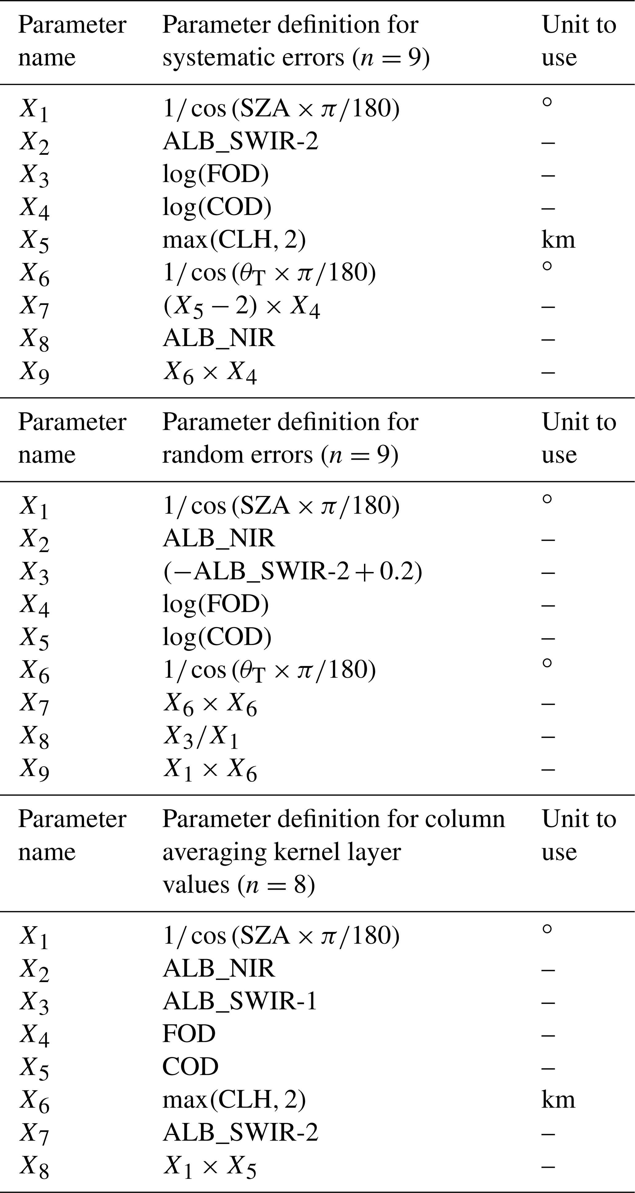
Figure 10 also shows $X_{{\mathrm{CO}}_{\mathrm{2}}}$ and $X_{{\mathrm{CH}}_{\mathrm{4}}}$ random errors for the with-SPEX design scenario, those are lower than in the no-SPEX design scenario. Indeed, due to the GHG and aerosol information entanglement shown in Sect. 5.1, the better a priori constraint of aerosol parameters brought by SPEXone enables the dedication of more of the NanoCarb measurement information to the estimation of GHG parameters in the with-SPEX scenario. For nearly all the atmospheric and observational situations considered in this work, $X_{{\mathrm{CO}}_{\mathrm{2}}}$ and $X_{{\mathrm{CH}}_{\mathrm{4}}}$ satisfactorily reach the SCARBO precision objectives of below 1 ppm and 6 ppb, respectively.

Table 5 Parameterisation approximation errors.

6 Level 2 performance parameterisation

6.1 Linear regressions

In order to yield generalised SCARBO L2 performance models from the 324 situations considered in this work, we adopt the approach used in Buchwitz et al. (2013) and perform linear regressions to parameterise L2 performance results. In other words, we determine the c and a_i coefficients so that

$$\begin{array}{}\text{(4)}& Y=c+{\sum }_{i=\mathrm{1}}^n{a}_i{X}_i,\end{array}$$

with Y being an L2 performance result to parameterise as a function of n heuristically determined (linear and non-linear) parameters X_i, expressed as combinations of the selected ALB, SZA, CLH, COD and FOD parameters, and θ_T being the transversal angle position (absolute value) within the swath. Considering ALB_NIR, ALB_SWIR-1 and ALB_SWIR-2, which describe albedo model values at 0.7, 1.6 and 2.0 µm, respectively, Table 4 lists the X_i parameters used for $X_{{\mathrm{CO}}_{\mathrm{2}}}$ and $X_{{\mathrm{CH}}_{\mathrm{4}}}$ systematic errors, random errors and AK level value parameterisations.

Figure 11 shows parameterisation results for $X_{{\mathrm{CO}}_{\mathrm{2}}}$ systematic and random errors and for no-SPEX and with-SPEX design scenarios. For no-SPEX situations, results are parameterised for retrieved $\text{COD}+\text{FOD}<\mathrm{0.25}$ in order to emulate some sort of sensible filtering that could be performed in operational processing. For systematic errors, the parameterisation captures the combined COD, SZA and CLH trends of L2 results, as well as some of the transversal angle position dependence. Regarding no-SPEX random errors, the parameterisation captures the combined albedo and SZA trends (except for soil albedo at SZA =70^∘) but fails to reproduce the COD trend over vegetation and soil albedo situations due to the strong influence of this trend in desert situations. The transversal angle position dependence is well captured. The parameterisation for the with-SPEX scenario random errors is quite accurate and satisfactorily reproduces most of the L2 performance trends (for this scenario, we only filter with COD<0.6 and FOD<0.6). In addition, it can be noted that vegetation albedo situations, the most representative of European surface, are those for which parameterisations best reproduce the computed exact L2 performance. Similar results are obtained for $X_{{\mathrm{CH}}_{\mathrm{4}}}$ (see the Supplement, where AK parameterisation results are also shown). Overall, the means and standard deviations of parameterisation approximation errors evaluated for all 324 situations and transversal angle positions that passed filters are given in Table 5.

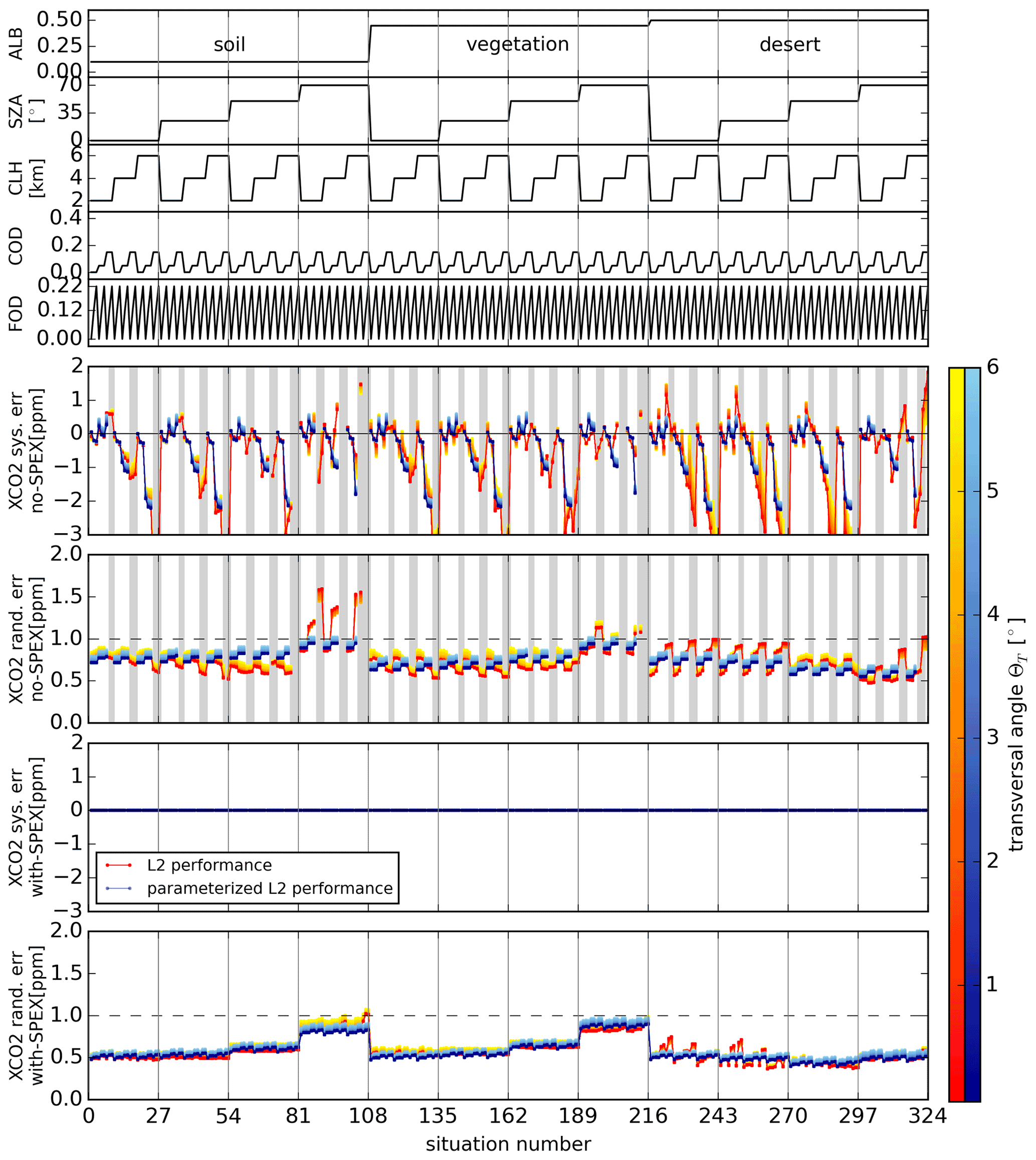
Figure 11 Parameterised (blue colour scale) NanoCarb $X_{{\mathrm{CO}}_{\mathrm{2}}}$ systematic (sixth and eighth panels) and random errors (seventh and ninth panels) compared to exact L2 error retrieval results (red colour scale). Results are plotted as a function of the situation number: the five top panels detail the ALB (0.7 µm), SZA, CLH, COD and FOD values defining all 324 situations. Grey-shaded areas denote situations for which retrievals did not satisfactorily converge or situations that were filtered out according to the retrieved COD and FOD values.

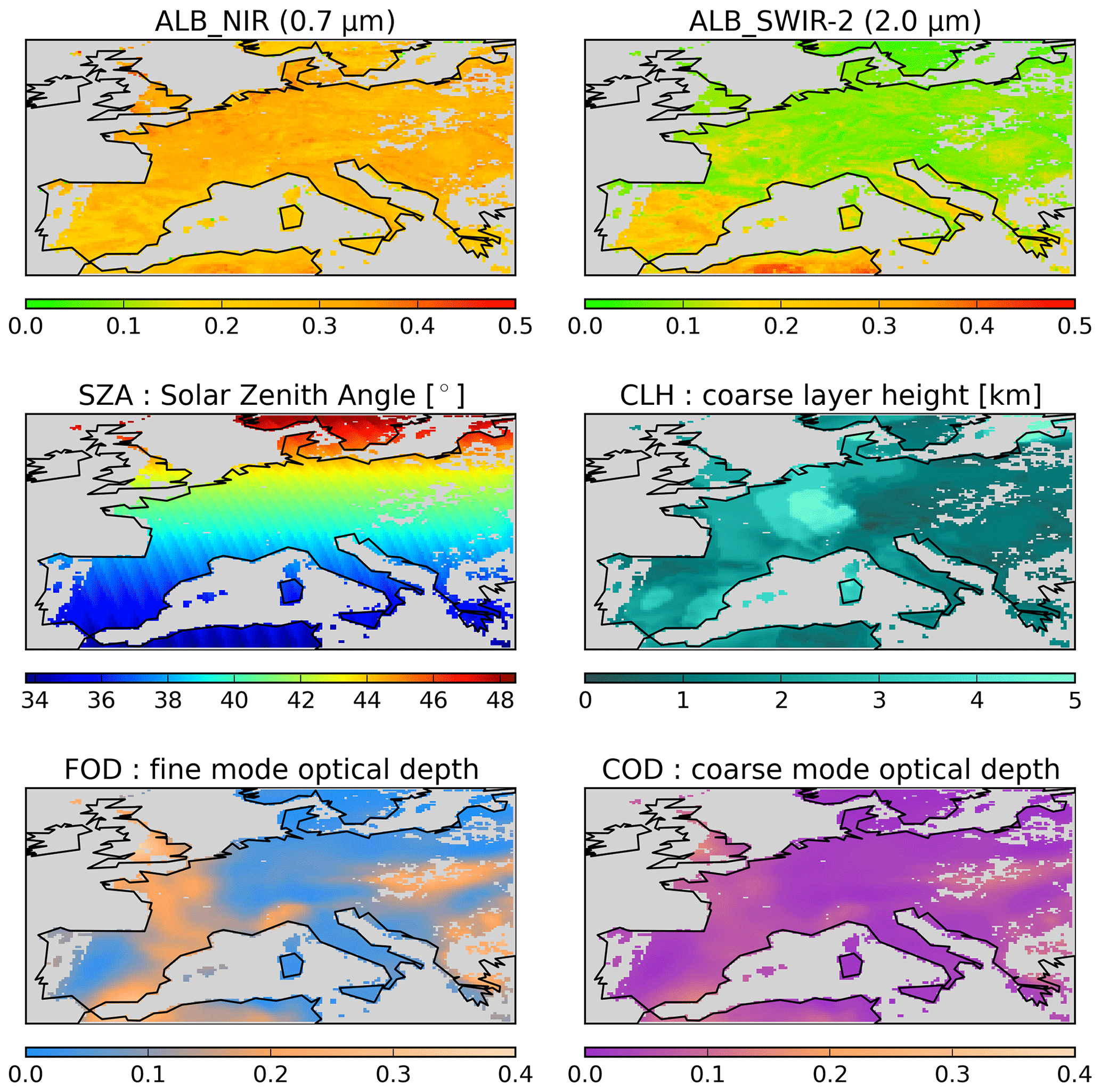
Figure 12 ALB_NIR, ALB_SWIR-2, SZA, CLH, FOD and COD cloud-free parameter maps of 1 July 2015, averaged on a $\mathrm{0.2}{}^{\circ }\times \mathrm{0.2}{}^{\circ }$ grid.

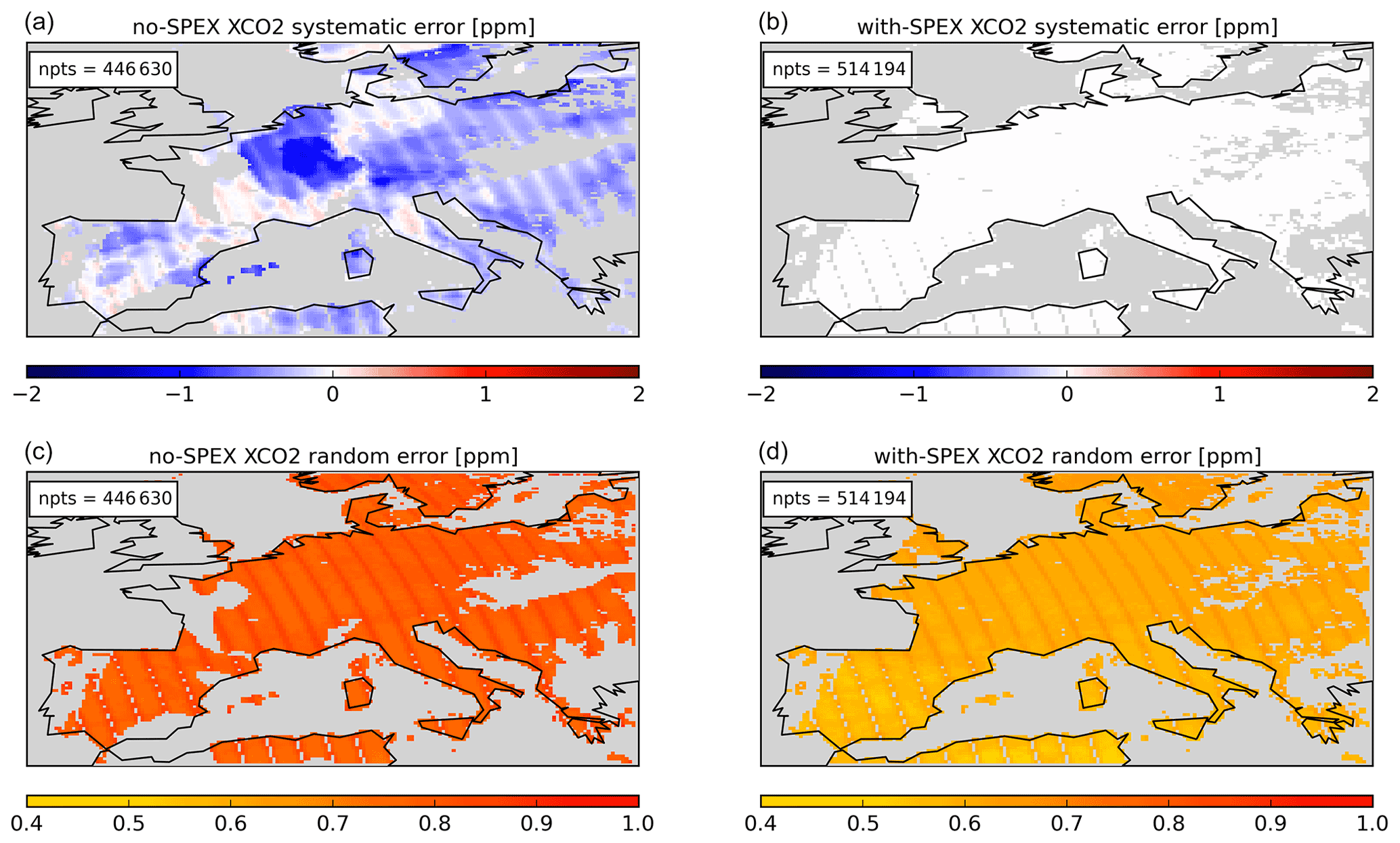
Figure 13 Parameterised $X_{{\mathrm{CO}}_{\mathrm{2}}}$ systematic (a, b) and random (c, d) errors for 1 July 2015 for the no-SPEX (a, c) and with-SPEX (b, d) design scenario cases and averaged on a $\mathrm{0.2}{}^{\circ }\times \mathrm{0.2}{}^{\circ }$ grid.

6.2 Application of L2 performance parameterisations: 1 July 2015 example

SCARBO ground tracks are calculated and auxiliary datasets are gathered to provide large spatial and temporal scale maps of the five selected error-critical parameters: ALB (at 0.7, 1.6 and 2.0 µm), SZA, CLH, COD and FOD. We then use those maps to apply the previously obtained L2 performance parameterisations and yield systematic and random $X_{{\mathrm{CO}}_{\mathrm{2}}}$ and $X_{{\mathrm{CH}}_{\mathrm{4}}}$ errors, as well as $X_{{\mathrm{CO}}_{\mathrm{2}}}$ and $X_{{\mathrm{CH}}_{\mathrm{4}}}$ column-averaging kernels, which can then be used for L4 flux inversion studies.

The SCARBO constellation considered in this study for the ground track computation is composed of 28 satellites on sun-synchronous orbits of 605.498 km height and separated into two orbital planes: one observing at 10:00 LT and the second at 14:00 LT. Orbital parameters are adjusted to have a repeating cycle of 7 d so that the second plane repeats the ground traces of the first one. As the provided L2 performance results already include the contribution of all along-track NanoCarb measurements, observations are sampled at the resolving spatial resolution of ∼2.3 km in the across-track direction, producing 85 soundings in a 200 km swath corresponding to transversal angle positions θ_T between 0^∘ in 9^∘ in absolute value.

Only clear-sky land observations are kept: cloud flagging is performed with the MODIS Atmosphere L2 Cloud Mask Product (Ackerman and Frey, 2015a, b) and land/sea flagging with the Global Multi-resolution Terrain Elevation Data (GMTED2010) 30 arcsec product (Danielson and Gesch, 2011). Given the date and time, the derived observation geolocations make it possible to yield the SZA dataset.

Aerosol parameters COD, FOD and CLH are generated using the T255 Copernicus Atmospheric Monitoring Service (CAMS) reanalyses for aerosols (Flemming et al., 2017) interpolated at 15 arcsec resolution. The different aerosol types proposed in this product are separated into two classes, a fine mode and a coarse mode, according to their overall size. Coarse-mode and fine-mode optical depths (COD and FOD) datasets are then generated by summing the optical depths of the individual types belonging to each class. Finally, CAMS vertical mixing ratios of aerosol types classified as coarse are processed to yield the average mass altitude that is used for the CLH dataset.

In order to create a ground albedo dataset at our three reference wavelengths, we employ the ESA ADAM (A Surface Reflectance Database for ESA's Earth Observation Missions) climatology (Bacour et al., 2020) that relies on MODIS surface reflectance data. In order to extrapolate reflectance values at our three reference wavelengths, the Étude CLImatologique des Propriétés optiques de fonds de Sol (ECLIPS) French Agence Nationale de la Recherche (ANR) project data are used (mentioned in Bacour, 2019), finally yielding ALB_NIR, ALB_SWIR-1 and ALB_SWIR-2 parameter datasets.

In order to illustrate the application of the L2 performance parameterisations, we use the parameter datasets of 1 July 2015 to compute parameterised $X_{{\mathrm{CO}}_{\mathrm{2}}}$ systematic and random errors for the 10:00 LT orbital plane satellites for both no-SPEX and with-SPEX design scenarios. Figure 12 shows $\mathrm{0.2}{}^{\circ }\times \mathrm{0.2}{}^{\circ }$ averaged ALB_NIR, ALB_SWIR-2, SZA, CLH, COD and FOD cloud-free parameter maps. Unsurprisingly, albedo values are mostly representative of vegetation models (see Fig. 5), with rather high reflectance near 0.7 µm and low reflectance near 2.0 µm. Southern Spain and Italy and the Maghreb have more desert-like surface albedos. For 1 July 2015, CAMS-simulated aerosols are mostly present over the Maghreb, eastern Spain, France, the United Kingdom and eastern Europe, with rather high fine-mode optical depth and low coarse-mode optical depths. These coarse-mode aerosols have a rather low layer altitude, except over Germany, where a low COD layer reaches nearly 5 km. Figure 13 shows the corresponding parameterised $X_{{\mathrm{CO}}_{\mathrm{2}}}$ systematic and random errors for both design scenarios (see the Supplement for $X_{{\mathrm{CH}}_{\mathrm{4}}}$). These are computed for transversal angle positions lower than 6^∘ in absolute values, as we do not consider the full NanoCarb swath in this work. Soundings are filtered with $\text{COD}+\text{FOD}<\mathrm{0.25}$ and COD<0.6 and FOD<0.6 in no-SPEX and with-SPEX scenario cases, respectively, which explains the different number of soundings between these two scenarios. No-SPEX systematic errors mostly correlate with COD and CLH as already noted in Fig. 7., whereas no systematic error is given for with-SPEX scenario as per its hypotheses. Regarding random errors, they are lower in the with-SPEX scenario and decrease over more desert-like albedo situations, as can be seen in southern Spain and Italy and the Maghreb. Finally, the stripping that can be noticed on random error maps corresponds to the loss of precision with the transversal position within the swath, as |θ_T| gets closer to 6^∘.

7 Conclusions

In this work, we have carried out the Level 2 performance assessment of the NanoCarb concept developed in the SCARBO project. For a set of 324 scattering-error-critical atmospheric and observational situations, we retrieved $X_{{\mathrm{CO}}_{\mathrm{2}}}$ and $X_{{\mathrm{CH}}_{\mathrm{4}}}$ directly from NanoCarb truncated interferograms by using the 5AI inverse scheme.

First, as this concept constitutes an original approach to NIR and SWIR infrared measurements compared to state-of-the-art GHG satellite missions, we have analysed the vertical sensitivities and information content of the truncated interferograms. Retrievals are clearly sensitive to CO₂ and CH₄ with degrees of freedom close to 1.0, and the retrieved $X_{{\mathrm{CO}}_{\mathrm{2}}}$ and $X_{{\mathrm{CH}}_{\mathrm{4}}}$ are representative of all atmospheric layers as with usual NIR and SWIR concepts.

In order to establish the merits of coupling NanoCarb with the SPEXone instrument dedicated to aerosols, we have compared the results for two SCARBO satellite design scenarios: no-SPEX and with-SPEX. Systematic $X_{{\mathrm{CO}}_{\mathrm{2}}}$ and $X_{{\mathrm{CH}}_{\mathrm{4}}}$ retrieval errors originating from the presence of fine-mode aerosols on the optical path can be significantly reduced by taking advantage of NanoCarb coupling with SPEXone. In addition, the performance of SPEXone for coarse-mode aerosols also enables the reduction of systematic $X_{{\mathrm{CO}}_{\mathrm{2}}}$ errors where they are the largest, e.g. for a typical European vegetation albedo situation with SZA =50^∘ and high COD. Desert situations with low SZAs may still remain a challenge in case of transient desert dust contaminations for instance.

Regarding precision, $X_{{\mathrm{CO}}_{\mathrm{2}}}$ and $X_{{\mathrm{CH}}_{\mathrm{4}}}$ random errors span 0.5–1 ppm and 4–6 ppb, respectively. Thus, for transversal angle positions lower than 6^∘, NanoCarb is compliant with the 1 ppm and 6 ppb precision objectives for $X_{{\mathrm{CO}}_{\mathrm{2}}}$ and $X_{{\mathrm{CH}}_{\mathrm{4}}}$, respectively, for situations with SZA ≤50^∘.

These systematic and random retrieval column errors, as well as their vertical sensitivities, have been successfully parameterised as functions of the five selected scattering-error-critical parameters. Consequently, large L2 maps can be produced and distributed for L4 atmospheric GHG flux inversion performance assessments.

This simulation study sheds light on the Level 2 performance of the peculiar NanoCarb truncated interferogram concept: it exhibits an interesting potential for providing meaningful information about greenhouse gas atmospheric concentrations, with a very compact imaging spectrometer. As for all simulation studies, there are implicit hypotheses that need to be considered: only scattering-error-critical situations have been considered, and prior knowledge of the true synthetic state of the atmosphere and of the surface is assumed to be perfect but for aerosol parameters in the no-SPEX scenario. In particular, the number of aerosol types, their optical properties and their number of layers are considered to be exactly known. In addition, the instrumental model is also ideal: it implements the theoretical Fabry–Pérot interferometer equations without considering any miscalibrated optical defect. However, as the SCARBO concept (NanoCarb coupled with SPEXone) reaches and even outperforms its precision objectives in this work with ideal hypotheses, we can expect some margins to cover for possible instrumental parameter imprecisions. This would be a next step towards an ultimately complete error budget that takes into account the critical instrumental (L1) and retrieval setup (L2) parameters that impact the overall performance of the SCARBO concept.

This first step in assessing NanoCarb L2 performance has also enabled us to point out geophysical variable information entanglements in NanoCarb truncated interferograms when examining the retrieval degrees of freedom. These include entanglements between albedo and surface pressure, albedo and CO₂, albedo and CH₄, and finally CH₄ and H₂O that had not been taken into account for the NanoCarb optimised OPD selection and model used in this work. Because of the very nature of NanoCarb measurements, these entanglements also evolve within the FOV, leading to an increase in $X_{{\mathrm{CO}}_{\mathrm{2}}}$ and $X_{{\mathrm{CH}}_{\mathrm{4}}}$ random errors on the swath edges. This specificity impacts the achievable swath for a given precision objective. It is consequently critical for the design of the SCARBO constellation, which results from a compromise between the number of satellites, the coverage and the revisit possibilities. Thus, by identifying the limits to disentangled GHG sensitivity within NanoCarb truncated interferograms, this work has also paved the way for future improvements of the whole concept design.

Appendix A: Combining NanoCarb measurements in the along-track dimension

With its current design, the NanoCarb instrument can gather up to n=102 independent truncated interferograms over the same exact fixed ground location. It corresponds to a unique state of the atmosphere that we seek to estimate from all the available measurements. Algorithmically speaking, using the Rodgers (2000) notation and following his guidance in Sect. 4.1.1, this can be achieved by including all n NanoCarb truncated interferograms inside the same measurement vector $\mathit{y}=\left[{\mathit{y}}_{\mathbf{1}},\mathrm{\dots },{\mathit{y}}_{\mathit{n}}\right]$ to retrieve one unique posterior state $\widehat{\mathit{x}}$. This posterior state maximises the probability $P\left(\mathit{x}\mathrm{|}{\mathit{y}}_{\mathbf{1}},\mathrm{\dots },{\mathit{y}}_{\mathit{n}}\right)$ that can be expressed with Bayes' theorem because measurements y_i are independent, as shown by the following equation.

$$\begin{array}{}\text{(A1)}& \begin{array}{rl}P\left(\mathit{x}\mathrm{|}{\mathit{y}}_{\mathbf{1}},\mathrm{\dots },{\mathit{y}}_{\mathit{n}}\right)=& {\displaystyle \frac{P\left({\mathit{y}}_{\mathbf{1}},\mathrm{\dots },{\mathit{y}}_{\mathit{n}}\mathrm{|}\mathit{x}\right)P\left(\mathit{x}\right)}{P({\mathit{y}}_{\mathbf{1}},\mathrm{\dots },{\mathit{y}}_{\mathit{n}})}}\\ =& P\left(\mathit{x}\right){\prod }_{i=\mathrm{1}}^n{\displaystyle \frac{P\left({\mathit{y}}_{\mathit{i}}\mathrm{|}\mathit{x}\right)}{P\left({\mathit{y}}_{\mathit{i}}\right)}}\end{array}\end{array}$$

Assuming Gaussian statistics for both state and measurements and a linear forward model described by its Jacobian matrices K_i corresponding to the measurement y_i, we can express the a posteriori covariance matrix $\widehat{\mathbf{S}}$ of the unique posterior state $\widehat{\mathit{x}}$ as follows:

$$\begin{array}{}\text{(A2)}& \widehat{\mathbf{S}}={\left[{{\mathbf{S}}_{\mathbf{a}}}^{-\mathrm{1}}+{\sum }_{i=\mathrm{1}}^n{{\mathbf{K}}_{\mathbf{i}}}^{\mathbf{T}}{{\mathbf{S}}_{\mathbf{e},\mathbf{i}}}^{-\mathbf{1}}{\mathbf{K}}_{\mathbf{i}}\right]}^{-\mathrm{1}},\end{array}$$

where S_a is the a priori covariance matrix of the a priori state vector x_a and S_e,i is the a priori covariance matrix of the individual measurement y_i. At the same time, for all individual a posteriori states ${\widehat{\mathit{x}}}_i$ retrieved from the individual independent measurements y_i, their a posteriori covariance matrix ${\widehat{\mathbf{S}}}_i$ can be expressed as follows:

$$\begin{array}{}\text{(A3)}& {\widehat{\mathbf{S}}}_i={\left[{{\mathbf{S}}_{\mathbf{a}}}^{-\mathbf{1}}+{{\mathbf{K}}_{\mathbf{i}}}^{\mathbf{T}}{{\mathbf{S}}_{\mathbf{e},\mathbf{i}}}^{-\mathbf{1}}{\mathbf{K}}_{\mathbf{i}}\right]}^{-\mathrm{1}}.\end{array}$$

Thus, using Eqs. (A2) and (A3) we can express $\widehat{\mathbf{S}}$ as a function of individual a posteriori covariance matrices ${\widehat{\mathbf{S}}}_i$:

$$\begin{array}{}\text{(A4)}& {\widehat{\mathbf{S}}}^{-\mathrm{1}}={{\mathbf{S}}_{\mathbf{a}}}^{-\mathbf{1}}+{\sum }_{i=\mathrm{1}}^n\left({\widehat{\mathbf{S}}}_i^{-\mathrm{1}}-{{\mathbf{S}}_{\mathbf{a}}}^{-\mathbf{1}}\right).\end{array}$$

Regarding the unique a posteriori state $\widehat{\mathit{x}}$, we have

$$\begin{array}{}\text{(A5)}& \widehat{\mathit{x}}={\mathit{x}}_{\mathrm{a}}+\widehat{\mathbf{S}}{\sum }_{i=\mathrm{1}}^n{{\mathbf{K}}_{\mathbf{i}}}^{\mathbf{T}}{{\mathbf{S}}_{\mathbf{e},\mathbf{i}}}^{-\mathbf{1}}\left({\mathit{y}}_{\mathit{i}}-{\mathbf{K}}_{\mathbf{i}}{\mathit{x}}_{\mathit{a}}\right),\end{array}$$

and (at the same time) individual a posteriori states ${\widehat{\mathit{x}}}_i$ retrieved from the individual independent measurements y_i also verify the following equation:

$$\begin{array}{}\text{(A6)}& {\widehat{\mathit{x}}}_i={\mathit{x}}_{\mathit{a}}+{\widehat{\mathbf{S}}}_i{{\mathbf{K}}_{\mathbf{i}}}^{\mathbf{T}}{{\mathbf{S}}_{\mathbf{e},\mathbf{i}}}^{-\mathbf{1}}\left({\mathit{y}}_{\mathit{i}}-{\mathbf{K}}_{\mathbf{i}}{\mathit{x}}_{\mathit{a}}\right).\end{array}$$

Thus, using Eqs. (A5) and (A6), we can express $\widehat{\mathit{x}}$ as a function of individual a posteriori states ${\widehat{\mathit{x}}}_i$:

$$\begin{array}{}\text{(A7)}& {\widehat{\mathbf{S}}}^{-\mathrm{1}}\left(\widehat{\mathit{x}}-{\mathit{x}}_{\mathit{a}}\right)={\sum }_{i=\mathrm{1}}^n{\widehat{\mathbf{S}}}_i^{-\mathrm{1}}\left({\widehat{\mathit{x}}}_i-{\mathit{x}}_{\mathit{a}}\right).\end{array}$$

In conclusion, assuming all individual a posteriori state vectors ${\widehat{\mathit{x}}}_i$ are obtained with their respective posterior covariance matrices ${\widehat{\mathbf{S}}}_i^{-\mathrm{1}}$, Eqs. (A4) and (A7) explain how to combine them in order to compute the unique posterior state $\widehat{\mathit{x}}$ and its covariance matrix $\widehat{\mathbf{S}}$.