Complementing XCO₂ imagery with ground-based CO₂ and ¹⁴CO₂ measurements to monitor CO₂ emissions from fossil fuels on a regional to local scale

Various satellite imagers of the vertically integrated column of carbon dioxide (XCO₂) are under development to enhance the capabilities for the monitoring of fossil fuel (FF) CO₂ emissions. XCO₂ images can be used to detect plumes from cities and large industrial plants and to quantify the corresponding emission using atmospheric inversions techniques. However, this potential and the ability to catch the signal from more diffuse FF CO₂ sources can be hampered by the mix between these FF signals and a background signal from other types of CO₂ surface fluxes, and in particular of biogenic CO₂ fluxes. The deployment of dense ground-based air-sampling networks for CO₂ and radiocarbon (¹⁴CO₂) could complement the spaceborne imagery by supporting the separation between the fossil fuel and biogenic or biofuel (BF) CO₂ signals. We evaluate this potential complementarity with a high-resolution analytical inversion system focused on northern France, western Germany, Belgium, Luxembourg, and a part of the Netherlands and with pseudo-data experiments. The inversion system controls the FF and BF emissions from the large urban areas and plants, in addition to regional budgets of more diffuse emissions or of biogenic fluxes (NEE, net ecosystem exchange), at an hourly scale over a whole day. The system provides results corresponding to the assimilation of pseudo-data from a single track of a 300 km swath XCO₂ imager at 2 km resolution and from surface ground-based CO₂ and/or ¹⁴CO₂ networks. It represents the diversity of ¹⁴CO₂ sources and sinks and not just the dilution of radiocarbon-free FF CO₂ emissions. The uncertainty in the resulting FF CO₂ emissions at local (urban area/plant) to regional scales is directly derived and used to assess the potential of the different combinations of observation systems. The assimilation of satellite observations yields estimates of the morning regional emissions with an uncertainty down to 10 % (1σ) in the satellite field of view, from an assumed uncertainty of 15 % in the prior estimates. However, it does not provide direct information about emissions outside the satellite field of view or about afternoon or nighttime emissions. The co-assimilation of ¹⁴CO₂ and CO₂ surface observations leads to a further reduction of the uncertainty in the estimates of FF emissions. However, this further reduction is significant only in administrative regions with three or more ¹⁴CO₂ and CO₂ sampling sites. The uncertainty in the estimates of 1 d emission in North Rhine-Westphalia, a region with three sampling sites, decreases from 8 % to 6.6 % when assimilating the in situ ¹⁴CO₂ and CO₂ data in addition to the satellite data. Furthermore, this additional decrease appears to be larger when the ground stations are close to large FF emission areas, providing an additional direct constraint for the estimate of these sources rather than supporting the characterization of the background signal from the NEE and its separation from that of the FF emissions. More generally, the results indicate no amplification of the potential of each observation subsystem when they are combined into a large observation system with satellite and surface data.

1 Introduction

Article 4 of the Paris Climate Agreement aims to reduce greenhouse gas (GHG) emissions within a few decades on the basis of equity, until they are compensated for by GHG removals. The monitoring of this international ambition implies some operational observation of the GHG emissions, in particular those of carbon dioxide (CO₂) from fossil fuels (FFs). A significant contribution to this monitoring is expected from observations of atmospheric composition and atmospheric inversion systems (IPCC, 2019; European Commission et al., 2016; Pinty et al., 2017). In particular, the development of spaceborne imagery of the vertically integrated column of CO₂ (XCO₂), at spatial resolution better than 5 km, should make it possible to detect plumes downwind from anthropogenic sources of CO₂ (Pillai et al., 2016; Schwandner et al., 2017; Broquet et al., 2018). A key example of such imagery is the Copernicus Anthropogenic Carbon Dioxide Monitoring (CO2M; Pinty et al., 2017; Kuhlmann et al., 2019; Lespinas et al., 2020) constellation, which is scheduled to launch in 2025–2026. Each satellite of the constellation will observe XCO₂ with a ∼ 300 km swath and a ∼ 2 × 2 km² spatial resolution.

Previous analyses of the potential of high-resolution satellite imagery of XCO₂ (such as ESA, 2015; Wang et al., 2020; Santaren et al., 2021) have focused on its use as a stand-alone observation system and on the potential complementarity of images of co-emitted species co-registered with an instrument on board the same satellite or from another mission (Reuter et al., 2019; Kuhlmann et al., 2019, 2020). However, the distinction between FF and natural CO₂ signals and thus the separation between the FF and natural components in the flux estimates remain difficult, even when using high-resolution images and satellite data on co-emitted species (Kuhlmann et al., 2020; Santaren et al., 2021; Sadiq et al., 2021). The separation between the emissions from biofuel (BF) and FF combustion is another challenge because BF emissions can be located in the same hotspots as FF ones (Ciais et al., 2020).

The deployment of dense ground-based networks of near-surface air sampling for radiocarbon (¹⁴CO₂) has also been considered as a complement to the spaceborne imagery (European Commission et al., 2016). Indeed FF-emitted CO₂ is radiocarbon-free (Pinty et al., 2017; Levin et al., 2003, 2021): ¹⁴CO₂ surface data have a less ambiguous sensitivity to the signal from FF emissions than CO₂ surface data. However, practical constraints lead to sampling ¹⁴CO₂ daily if not weekly to monthly (Levin et al., 2020). This prevents the direct identification of temporal variations at higher frequencies, e.g. hourly, associated with the signal from cities and point sources, but time series of continuous hourly measurements of CO₂ should enable these specific temporal variations to be captured. Various studies have been conducted to estimate the potential of ¹⁴CO₂ surface data in addition to CO₂ surface data to discriminate anthropogenic from biogenic CO₂. Most of the studies with real samplings corresponded to local analyses (e.g. Levin et al., 2003; Turnbull et al., 2006; Lehman et al., 2013; Wenger et al., 2019; Lee et al., 2020). Inversions with pseudo-data were used to assess the potential of ¹⁴CO₂ surface data to monitor the FF CO₂ emissions at continental scales (Wang, 2016; Wang et al., 2018; Basu et al., 2016). However, Graven et al. (2018) or Basu et al. (2020) showed promising results regarding the quantification of budgets of FF CO₂ emissions or the assessment of their estimates from inventories based on ∼ 10 stations of ¹⁴CO₂ at the scale of California or of the United States, respectively.

This study aims at assessing the potential of a combination of a spaceborne XCO₂ imager and ground-based ¹⁴CO₂ and CO₂ networks to monitor FF emissions of CO₂ at finer spatial scales, typically that of administrative regions in Europe, and with a view to feed operational systems with highly accurate emission estimates. More specifically, it aims at assessing how these additional ground-based networks decrease the uncertainty in FF emissions by improving the distinction between the FF and biogenic fluxes.

There is currently no large-swath XCO₂ imager in orbit, and we assume that dense networks of ¹⁴CO₂, with more stations than the current ones even in areas relatively well equipped like Europe (Levin et al., 2020, https://www.icos-cp.eu/, last access: 25 August 2022), are required to support such monitoring of the FF CO₂ emissions. Furthermore, the combination of remote sensing data and air sample measurements has often been difficult, mainly due to systematic errors in satellite retrievals and in the atmospheric chemistry-transport models that simulate them. In this case, the air sample measurements are rather used to constrain some bias correction of the remote sensing data (Bergamaschi et al., 2009) and/or the model (Locatelli et al., 2015), or they are implicitly used to dampen the effect of these systematic errors. The gradual improvement in the quality of retrievals and models over time has just recently opened the door to a more harmonious use of remote sensing data and air sample measurements for inverse modelling (Byrne et al., 2022).

Therefore, this study relies on inversion tests performed with parameters corresponding to pseudo-observations and different scenarios of observation systems, i.e. on observing system simulation experiments (OSSEs). The analysis focuses on the strengths and limitations of the atmospheric sampling from the different measurement systems. It discards components of the uncertainties associated with the current atmospheric radiative transfer inversion systems, used to retrieve XCO₂ data from satellite measurements, and to the current atmospheric transport models underlying the atmospheric inversion. Our OSSEs include the simulation of the sampling of a CO2M-like spaceborne instrument from single orbits over western Europe at 12:00 (universal time coordinated, UTC) and a scenario of a dense CO₂ and ¹⁴CO₂ ground-based network.

The work performed relies on a Bayesian inversion framework, in which the knowledge of control parameters, here the CO₂ fluxes, improves with the assimilation of related observations. It is focused on the direct computation of the uncertainty in the control parameters. We analyse the uncertainty in the posterior values of the control parameters as a function of the observation system that is used for the inversion and the corresponding uncertainty reduction, i.e. the relative difference between the posterior uncertainty and the prior uncertainty in the control parameters. The analysis of this uncertainty reduction is made over 1 d at the local scale (urban areas, industrial plants) to the scale of administrative regions in Europe, following the rationale and the general inverse modelling framework of Santaren et al. (2021). It focuses on a large part of western Europe, using a regional atmospheric transport model with a 2 km horizontal zoom over northern France, western Germany, Belgium, Luxembourg, and a large part of the Netherlands.

The assimilation of ¹⁴CO₂ and CO₂ surface data in addition to XCO₂ images and the inclusion of non-FF fluxes of ¹⁴CO₂ in the inversion framework make use of the larger-scale inversion framework developed by Wang (2016). It takes into account not only the ¹⁴CO₂ emissions from nuclear power plants and fuel reprocessing plants but also the specific isotopic signatures of the heterotrophic respiration (HR) and net primary production (NPP) by land ecosystems (Miller et al., 2012; Basu et al., 2016, 2020) and thus solves for these fluxes separately. It also controls the emissions from BF burning.

The analytical inversion framework is described in Sect. 2. Results from the pseudo-data experiments with the assimilation of satellite observations alone are taken as a reference and presented in Sect. 3.1. Then a larger suite of experiments combining ¹⁴CO₂ and CO₂ surface and XCO₂ satellite observations is used to assess their complementarity in Sect. 3.2 to 3.3. Section 4 provides some discussions about this inversion framework and a conclusion regarding complementarity of XCO₂ satellite, ¹⁴CO₂, and CO₂ surface observations.

2 Methodology of the inversion

This section presents the high dimensional inversion framework designed in this study for the co-assimilation of CO₂ and ¹⁴CO₂ data. It has strong similarities with the system developed by Santaren et al. (2021), which assimilates CO₂ data only, and it borrows from Wang (2016) to assimilate ¹⁴CO₂ data. The system relies on the following.

• A local- to regional-scale analytical inversion framework (Wu et al., 2016) presented in Sect. 2.1, which controls anthropogenic emissions from large cities and industrial plants in addition to regional budgets of more diffuse emissions or of natural fluxes at hourly resolution (see the definition of the control vector in Sect. 2.5).

• A zoomed configuration of the regional atmospheric transport model CHIMERE (Menut et al., 2013) for most of western Europe, described in Sect. 2.2.

• Hourly to annual maps of all types of surface CO₂ and ¹⁴CO₂ fluxes, at high spatial resolution from the CO₂ Human Emissions project (CHE, https://www.che-project.eu/, last access: 25 August 2022), which are described in Sect. 2.3. They are used to distribute the local- to regional-scale budgets of the fluxes into corresponding high-resolution flux maps (see Sect. 2.5).

• Simulations of the locations and uncertainty of the XCO₂ retrievals and of the CO₂ and ¹⁴CO₂ ground-based data as a function of time, for different scenarios of the observing system, as described in Sect. 2.6. For the XCO₂ data, we rely on the simulation of the CO2M sampling during one satellite pass over the area of interest generated by the Institut für Umweltphysik Bremen (IUPB) in the frame of the ESA-PMIF project (European Spacial Agency, Plume Monitoring Inversion Framework Wang et al., 2020; Lespinas et al., 2020).

Inversions are conducted over a 1 d window from 00:00 to 24:00 UTC, on 1 July 2015, i.e. in summer when the biogenic fluxes are relatively high. The restriction to 1 d is connected to results of Santaren et al. (2021), which show the lack of sensitivity of observations made during a given day to the fluxes during other days over the modelling domain, and to the large computation cost associated with the preparation of a full day of analytical inversion. With such an inversion window, wider than the one chosen in Broquet et al. (2018) or Santaren et al. (2021), the system tracks the signal from the FF emissions up to 12 h before the satellite overpass (see Sect. 2.6.1) and 10 h before the in situ data assimilation window (see Sect. 2.6.2). After a few hours, the air masses having been transported over typically ∼ 30–100 km, and the signal from individual FF CO₂ sources (industrial plants, cities, regions) is much diffused and hardly detectable in XCO₂ images. Consequently this 1 d timescale is large enough to represent the full extent of the CO₂ FF plumes that can be exploited in images from CO2M-like instruments to compute the corresponding emissions (Broquet et al., 2018; Santaren et al., 2021). The ability to track large-scale budgets of FF emissions over longer time periods relies on complementary observations of FF emission tracers. These tracers, such as the ¹⁴CO₂ measurements considered here, may help filter a relatively low FF signal from the biogenic signal, which is generally much larger over long distances (Pinty et al., 2017; Palmer et al., 2006; Fortems-Cheiney et al., 2021; Sadiq et al., 2021). CO₂ and ¹⁴CO₂ ground-based networks could also reinforce the constraint on the FF CO₂ emission estimates during the few hours before the satellite overpass. By starting the inversion window 12 h before the satellite overpass and 10 h before the first surface measurement, we account for the full window of FF CO₂ emission, the estimate of which can potentially be directly constrained by these different datasets or by their combination.

2.1 Inversion general equation

Under the assumption that all uncertainties in the inversion problem have a Gaussian and unbiased distribution, these uncertainties are fully characterized by their covariance matrices. The inversion uses an observation operator to connect the control parameters (the flux budgets; see Sect. 2.5) to the observation vector (the space defined by the ensemble of pseudo-observations; see Sect. 2.6). Here, by construction, the observation operator is linear and is denoted H. On this basis, the analytical Bayesian inversion allows for the computation of the covariance matrix of the posterior uncertainty (uncertainty in the posterior estimate of the fluxes) A as a function of H, of the covariance matrix of the prior uncertainty (uncertainty in the prior estimate of the fluxes; see Sect. 2.5.2) B, and of the model and observation errors covariance matrix R (in the observation space; see Sect. 2.6.3), following Tarantola (2005):

$$\begin{array}{}\text{(1)}& \mathbf{\text{A}}={\left[{\mathbf{\text{B}}}^{-\mathrm{1}}+{\mathbf{\text{H}}}^T{\mathbf{\text{R}}}^{-\mathrm{1}}\mathbf{\text{H}}\right]}^{-\mathrm{1}}.\end{array}$$

The observation operator H is decomposed, following the notations of Staufer et al. (2016), into

$$\begin{array}{}\text{(2)}& \mathbf{\text{H}}={\mathbf{\text{H}}}_{\mathrm{sample}}{\mathbf{\text{H}}}_{\mathrm{transp}}{\mathbf{\text{H}}}_{\mathrm{distr}}.\end{array}$$

H_distr defines (i) the spatial and temporal distribution of the fluxes within each area corresponding to a control parameter and beyond the temporal resolution of these control parameters, (ii) the flux budgets to be rescaled by the inversion for these areas at the control resolution, and (iii) the application of the isotopic signatures to CO₂ fluxes. Here, this operator is based on the flux products and on the signatures described in Sect. 2.3.

H_transp is the atmospheric transport operator, corresponding to our configuration of the transport model CHIMERE described in Sect. 2.2.

H_sample corresponds to the computation of XCO₂ and to the sampling of XCO₂ or of near-ground mole fractions of CO₂ and ¹⁴CO₂ at the observation time and locations from the output of the CHIMERE model. Section 2.6 provides more details on this operator.

The H observation operator matrix is built explicitly to solve for Eq. (1) analytically, which requires an extensive set of simulations. The different columns of H correspond to the imprints in the observation space of the different control variables. They are computed by applying the sequence of operators H_distr, H_transp, and then H_sample to each control variable set to 1, keeping the others null (Broquet et al., 2018). In practice, the application of the H_transp operator corresponds to passive tracer transport simulations with the CHIMERE model which bears non-linearities that are assumed to be negligible (see Sect. 2.2.1) and thus that are assumed to be well emulated via the building of H. A generalized H matrix is actually stored for the analytical inversion system to anticipate any option for H_sample or for the control vector, by recording the full fields from the application of H_distr and H_transp to all control variables considered in this study.

By focusing on the analysis of uncertainties in the control parameters, this study requires the application of Eq. (1) but not the actual computation of emission estimates based on synthetic data. The computation of H is the main and most demanding step in the preparation of the inversion system. In addition to this computation, the application of Eq. (1) only requires the derivation of the B and R matrices, and the inversions of positive-definite matrices corresponding to the control space. This analytical expression of the inversion framework allows for the uncertainties in the individual control parameters or for budgets of emissions integrated in space or in time to be analysed and for many options for the observation system to be tested despite the dimension of the high-resolution inversion problem.

2.2 Atmospheric transport

2.2.1 Transport model configuration

The transport operator of CO₂ and ¹⁴CO₂ in the atmosphere, H_transp, relies on the CHIMERE transport model, driven here by the Community Inversion Framework (CIF, Berchet et al., 2021). The domain and the horizontal grid for the CHIMERE configuration used here are represented in Fig. 1. The domain covers a part of western Europe (longitude: −6.82 to 19.18^∘, latitude: 42.0 to 56.39^∘). The resolution of the horizontal grid varies between 50 and 2 km. The 2 km × 2 km resolution zoom covers northern France, Luxembourg, Belgium, a large part of the Netherlands, and western Germany (longitude: −1.25 to 10.64^∘, latitude: 47.45 to 53.15^∘). The vertical grid is composed of 29 pressure layers extending from the surface to 300 hPa (approximately 9 km above the ground level).

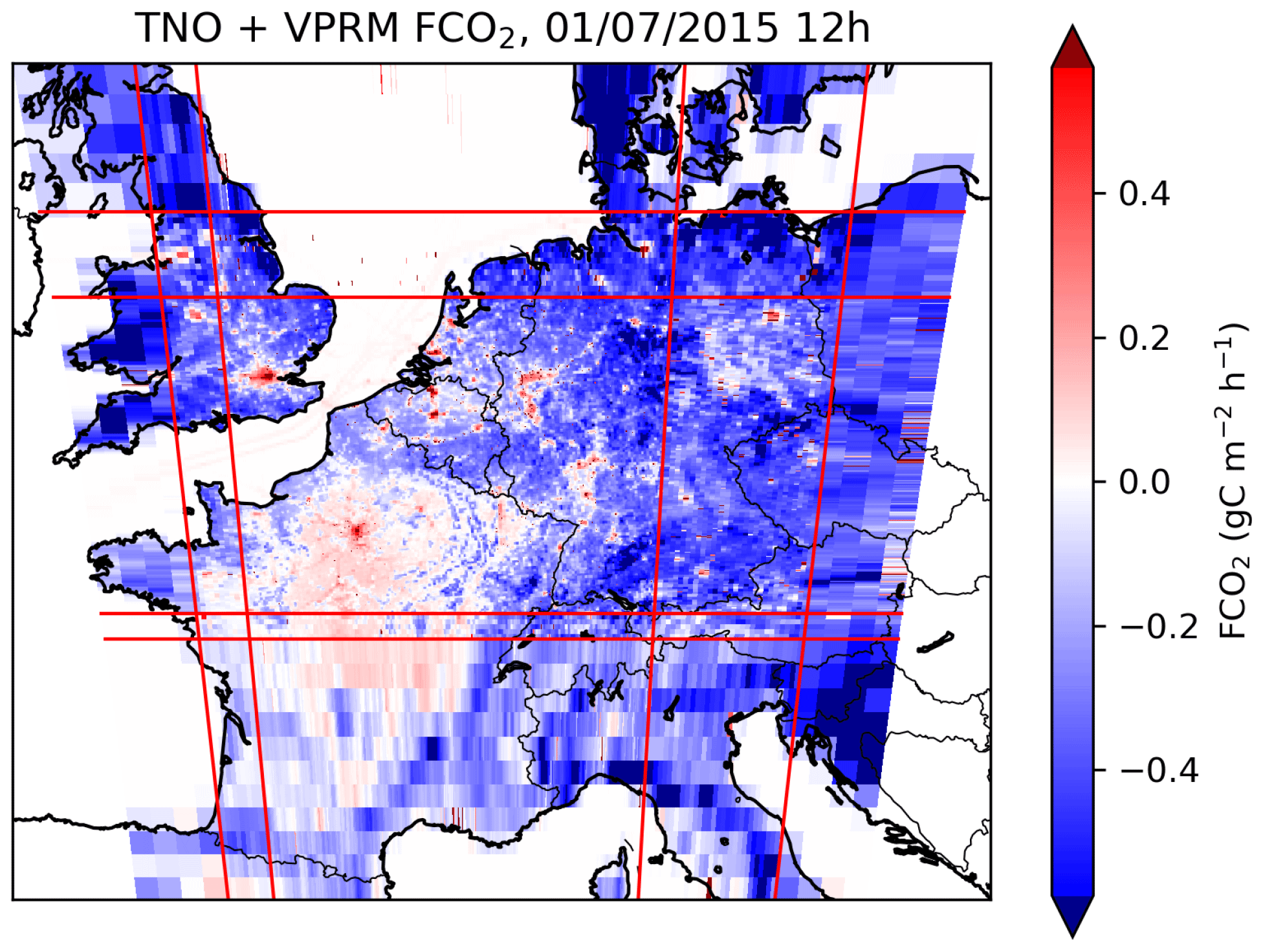
Figure 1 CO₂ flux map (based on values from the TNO inventory and VPRM simulations for 1 July 2015 at 12:00 UTC) over the atmospheric transport modelling grid. The red lines delimit the spatial resolution changes within the domain (from 2 to 10 km and then 50 km from the middle to the edges of the domain).

Our configuration of CHIMERE ignores chemistry since CO₂ and ¹⁴CO₂ are inert species at the timescale considered in this study (24 h). The actual transport of passive tracers is linear, but non-linearities arise in the models due to their inherent discretization of the transport. However, these non-linearities are small, and this explains why the resulting atmospheric transport operator is assumed to be well emulated via the building of the H matrix. CHIMERE is forced by meteorological variables provided by the European Centre for Medium-Range Weather Forecasts (ECMWF) for the CHE project at 9 km resolution (Agusti-Panareda, 2018). Figure 2 provides indications on the typical horizontal transport conditions during the day of inversions over the area of interest: on 1 July 2015, a southeast wind over the northeast part of the domain spreads the atmospheric signature of FF emissions in the northwest direction.

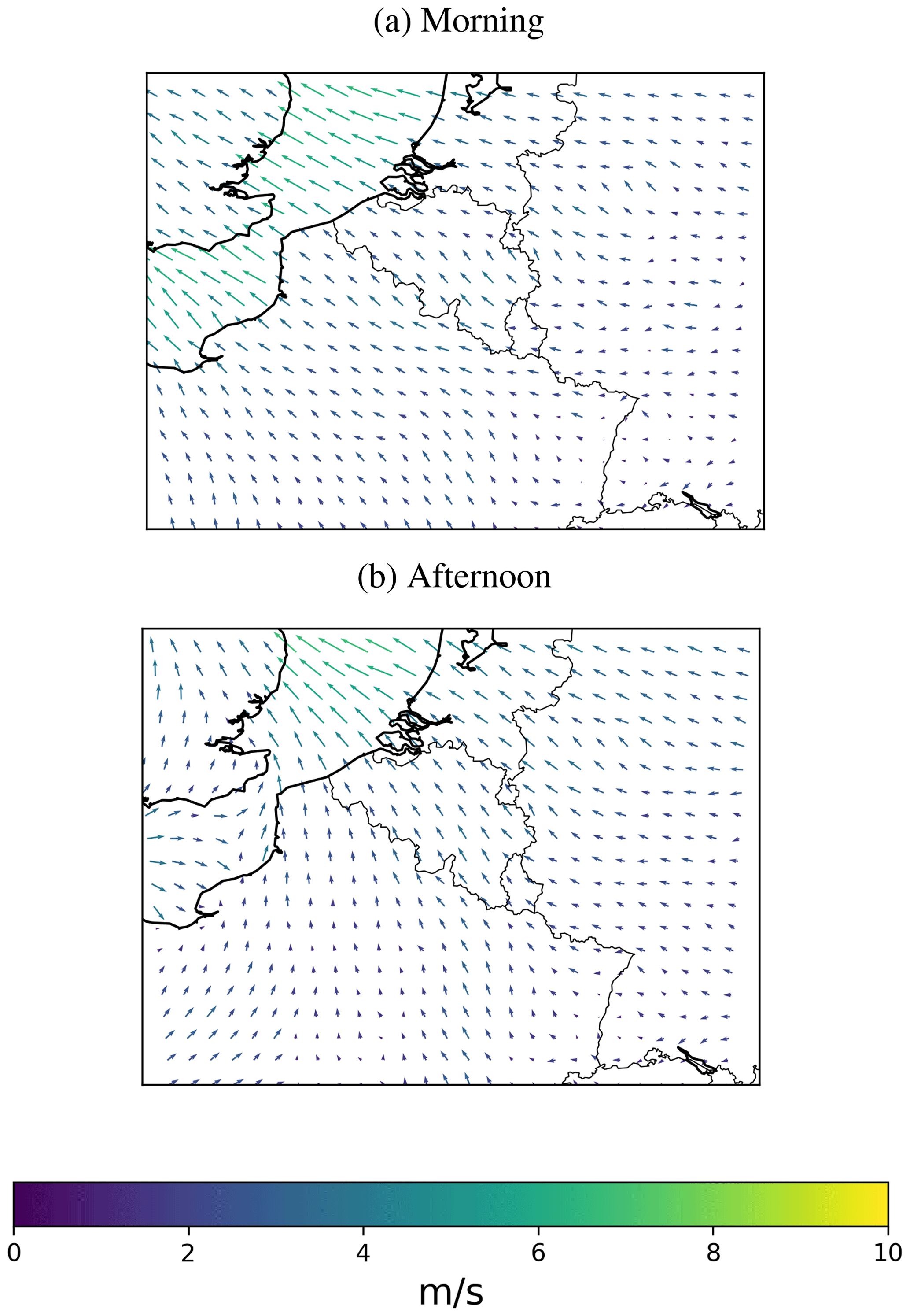
Figure 2 Morning (a) and afternoon (b) wind averaged in the first two vertical layers of the CHIMERE grid (i.e. heights between 0 and 28 m above the ground).

2.2.2 Simulation of CO₂ and ¹⁴CO₂ transport

In this section, we present a formal decomposition of the CO₂ and ¹⁴CO₂ transport in order to introduce the notation and assumptions used in the inversion framework. The decomposition of the ¹⁴CO₂ transport and its formulation in a specific unit (parts per million per mil, ppm ‰) follow that of Wang (2016).

$$\begin{array}{}\text{(3)}& {\displaystyle }{C}_{\mathrm{a}}={\mathbf{\text{H}}}_{\mathrm{transp}}{\displaystyle }\left[F_{\mathrm{FF}}+F_{\mathrm{BF}}+F_{\mathrm{NPP}}+F_{\mathrm{HR}}\right]+{\mathbf{\text{H}}}_{\mathrm{bc}}\left[C_{\mathrm{bc}}\right]\end{array}$$

$$\begin{array}{}\text{(4)}& \begin{array}{rl}{\displaystyle }{C}_{\mathrm{a}}\cdot {\mathit{\delta }}_{\mathrm{a}}={\mathbf{\text{H}}}_{\mathrm{transp}}& {\displaystyle }\left[{\mathit{\delta }}_{\mathrm{FF}}\cdot F_{\mathrm{FF}}+{\mathit{\delta }}_{\mathrm{BF}}\cdot F_{\mathrm{BF}}+\right.\\ {\displaystyle }& {\displaystyle }{\mathit{\delta }}_{\mathrm{NPP}}\cdot F_{\mathrm{NPP}}+{\mathit{\delta }}_{\mathrm{HR}}\cdot F_{\mathrm{HR}}+\\ {\displaystyle }& {\displaystyle }\left.\mathrm{1}/R_{\mathrm{std}}\cdot F_{\mathrm{Nucl}}\right]+\\ {\displaystyle }& {\displaystyle }{\mathbf{\text{H}}}_{\mathrm{bc}}\left[C_{\mathrm{bc}}\cdot {\mathit{\delta }}_{\mathrm{bc}}\right]\end{array}\end{array}$$

• C_a is the CO₂ atmospheric mole fraction.

• F_x terms correspond to different types x of CO₂ fluxes within the transport modelling domain: FF emissions, BF emissions, NPP, and HR. Of note is that the sign of fluxes in this equation corresponds to the atmosphere point of view: they are positive when CO₂ is emitted to the atmosphere and negative when it is absorbed from the atmosphere. In particular, F_NPP is positive when the NPP is negative.

• C_bc represents the boundary (top and lateral) and initial conditions of CO₂ mole fraction and H_bc their transport within the modelling domain, but they are ignored in this inversion study (see Sect. 2.3.3).

• δ_a represents the ${}^{\mathrm{14}}{\mathrm{CO}}_{\mathrm{2}}{/}^{\mathrm{12}}{\mathrm{CO}}_{\mathrm{2}}$ ratios in the atmosphere (R), normalized by the ${}^{\mathrm{14}}\mathrm{C}{/}^{\mathrm{12}}\mathrm{C}$ ratio in the modern standard ($(R/R_{\mathrm{std}}-\mathrm{1})$; $R_{\mathrm{std}}=\mathrm{1.176}\times {\mathrm{10}}^{-\mathrm{12}}$). Similarly, in the following, all δ values are also normalized ratios.

• δ_x represents the ¹⁴CO₂ isotopic signatures of the fluxes listed above.

• F_Nucl corresponds to ¹⁴CO₂ fluxes from nuclear power plants.

2.3 Flux maps

2.3.1 CO₂ flux maps

The anthropogenic CO₂ emissions, from both FF and BF combustion, are derived from two inventories of the annual emissions produced by the Netherlands Organisation for Applied Scientific Research (TNO) over Europe for the year 2015 (Denier van der Gon et al., 2017; Super et al., 2020). These inventories provide emission maps for 15 activity sectors following the Gridded Nomenclature For Reporting (GNFR) of the United Nations Framework Convention on Climate Change (UNFCCC). The emissions in the 2 km resolution area of the domain are interpolated from a ∼1 km (1/60^∘×1/120^∘) resolution inventory (TNO_GHGco_1×1km_v1_1), which entirely covers this area but not the whole CHIMERE domain (its extent being −2 to 19^∘ in longitude and 47 to 56^∘ in latitude). The emissions in the rest of the CHIMERE domain are interpolated from a ∼ 6 km (1/10^∘×1/20^∘) resolution inventory (TNO_GHGco_v1_1, covering −30 to 60^∘ in longitude and 30 to 72^∘ in latitude). These data are projected on the CHIMERE horizontal grid ensuring mass conservation. The temporal disaggregation at an hourly scale is based on coefficients provided with the TNO inventories for each sector of activity and as a function of the time zones provided in the CHE project (Marshall et al., 2019). Emissions from point sources are projected on the CHIMERE vertical grid with coefficients depending on the activity sectors (Bieser et al., 2011), also provided with the TNO inventories, while emissions from diffused sectors of activity (traffic, heating, etc.) are emitted from the ground in the model.

No distinctions between CO₂ BF emissions from woods and crops are made in the TNO inventories. However this split is needed to derive ¹⁴CO₂ fluxes (see below). Consequently, assumptions are made based on emission categories used in the TNO inventory. In this study, we consider that BF from woods is burned in power plants and in the industry and residential sectors only, i.e. in categories A to C. BF from crops is burned in categories F and L only, which correspond to road transport and agriculture. We assume that the BF emissions from the other sectors are negligible since they represent less than 2 % of the total BF emissions in the vast majority of countries.

The CO₂ biogenic fluxes are interpolated from simulations at 1 h and 5 km resolution with the VPRM model (Vegetation Photosynthesis and Respiration Model, Mahadevan et al., 2008) for the year 2015, provided by MPI-Jena over Europe (over latitude 31 to 68.7^∘, longitude −35.5 to 60.5^∘). The VPRM simulations provide estimates of gross primary production (GPP) and total respiration. However, we need to split the biogenic fluxes into NPP and HR since they bear different isotopic signatures. Therefore, we recombine GPP and respiration from VPRM into NPP and HR fluxes, using daily partition coefficients (α_HR) that are derived from ORCHIDEE-MICT simulations at 0.5^∘ resolution over Europe in 2015 (Guimberteau et al., 2018). The total biogenic fluxes correspond to the net ecosystem exchange (F_NEE=F_NPP + F_HR=F_GPP + F_Resp).

The total CO₂ fluxes for 1 July 2015 at 12:00 UTC are presented in Fig. 1.

2.3.2 Isotopic signatures and ¹⁴CO₂ flux maps

To produce ¹⁴CO₂ fluxes, corresponding isotopic signatures are applied to the CO₂ fluxes.

${\mathit{\delta }}_{\mathrm{FF}}=-\mathrm{1000}\mathrm{‰}$ was applied to F_FF for the whole year and domain.

We distinguish δ_BF,wood from δ_BF,crop because crops and wood have a different age at harvest, resulting in different ¹⁴C abundance. In a first approximation, we determined these δ_BF values as a spatial and temporal average of ¹⁴CO₂ content in vegetation, δ_biomass, simulated with the emulator of the ORCHIDEE-MICT model (Guimberteau et al., 2018; Naipal et al., 2018; Wang, 2016) over the whole ORCHIDEE-MICT Europe domain in 2015, selecting the relevant plant functional types (PFTs): non-tropical trees for δ_BF,wood and crops for δ_BF,crop. Such a computation of δ_BF relies on the hypothesis that the wood or crop fuel burnt in Europe comes from European (European Commission et al., 2017) and recently cut vegetation. As a result, ${\mathit{\delta }}_{\mathrm{BF},\mathrm{wood}}=\mathrm{95}$ ‰ and ${\mathit{\delta }}_{\mathrm{BF},\mathrm{crop}}=\mathrm{19}$ ‰.

δ_NPP monthly maps at 5 km spatial resolution were derived for application to the VPRM biogenic fluxes:

$$\begin{array}{}\text{(5)}& {\mathit{\delta }}_{\mathrm{NPP}}={\mathit{\delta }}_{\mathrm{a},\mathrm{surf}}-\mathit{ϵ},\end{array}$$

where δ_a,surf is the radiocarbon signature in the surface atmospheric layer and ϵ is the sum of kinetic and enzymatic ¹⁴CO₂ fractionation with respect to ¹²CO₂ depending on the C₃ or C₄ photosynthesis pathway of the vegetation.

Monthly background measurements of the radiocarbon ratio in the conventional definition (Δ¹⁴C, Stuiver and Polach, 1977) are available, in 2015, at Schauinsland in Germany (Hammer and Levin, 2017). The conversion to the normalized ratio, δ_a,surf, is done following Stuiver and Polach (1977), with ${\mathit{\delta }}_{{}^{\mathrm{13}}\mathrm{C}}$ from Graven et al. (2017). The resulting δ_a,surf varies between 46 ‰ and 49 ‰. Here, we neglect the impact of variations in this δ_a,surf at high spatial and temporal resolution on the ¹⁴CO₂ NPP fluxes themselves. Accounting for such variations for a precise computation of the δ_NPP, and so ¹⁴CO₂ NPP fluxes, would have required a dynamical computation with δ_a,surf depending on ¹⁴CO₂ mole fractions calculated by the transport model and would have introduced non-linearities. Accounting for such non-linearities in the observation operator would have required a complex inversion framework including the use of synthetic data and the iterative linearization of the observation operator into an evolving H matrix (Wang, 2016). However, over 1 d, these variabilities within each region and month are assumed to be negligible as was found by Wang (2016).

The value of ϵ is 36 ‰ for C₃ vegetation and 8 ‰ for C₄ vegetation as described by Wang (2016) from Farquhar et al. (1989) and Degens (1969). We derive the C₃–C₄ distribution on the VPRM grid and per month, from the combination of three land cover maps: the VPRM and ORCHIDEE land cover maps and monthly MIRCA2000 crop map (Portmann et al., 2010). This combination allows us to capitalize on the high spatial resolution of the VPRM land cover map at 5 km derived from SYNMAP at 1 km resolution (Jung et al., 2006) and a more precise PFT information in ORCHIDEE land cover maps at 0.5^∘ resolution to determine the C₃ or C₄ photosynthesis type. In the case of the crop PFT, the MIRCA2000 crop map at ∼ 0.08^∘resolution indicates the surface area covered by each crop type, and thus the relevant photosynthesis type, with a finer resolution than in ORCHIDEE and with the monthly variability of the year 2000. The resulting δ_NPP varies between 10 ‰ and 41 ‰.

δ_HR daily maps for the year 2015 are derived from simulations with the above-mentioned ORCHIDEE-MICT emulator. For each grid cell, the daily CO₂ and the corresponding ¹⁴CO₂ emissions from litter respiration and three types of soil respiration were aggregated. Their ratio, δ_HR, is then interpolated from the ORCHIDEE-MICT grid to the VPRM grid. The resulting δ_HR varies between 22 ‰ and 177 ‰.

Nuclear ¹⁴CO₂ emissions are calculated following Graven and Gruber (2011) based on the annual activity of each reactor, in 2015, reported in Zazzeri et al. (2018). For each reactor, activity data A in TBq yr⁻¹ is converted into ¹⁴C production in kg¹⁴C yr⁻¹:

$$\begin{array}{}\text{(6)}& F_{\mathrm{Nucl}}=A\times \mathit{\alpha }\times {\mathrm{10}}^{\mathrm{9}},\end{array}$$

with $\mathit{\alpha }=R_{\mathrm{std}}/\mathrm{0.226}$, where 0.226 Bq gC⁻¹ is the conversion factor from activity to carbon production.

2.3.3 Ignoring ocean fluxes, cosmogenic production, biomass burning emissions, and the regional boundary conditions

This study is focused on the analysis of uncertainties and of their propagation between the control and observation space. Therefore, the components that have to be taken into account in the transport simulation are those which bear uncertainties whose impact is accounted for or those which interfere with the transport of the components which bear uncertainties.

The impact of the uncertainties in the initial condition (at 00:00 UTC on 1 July 2015) and in the boundary conditions (at the lateral and top boundaries of the CHIMERE domain) are assumed to be negligible. The analysis by Santaren et al. (2021) suggests that the large-scale uncertainties should not have a large impact on the results, due to the good distinction between smooth background signal from the initial and boundary conditions and the imprints of the local and regional fluxes. Furthermore, the fine-scale uncertainties should have a limited impact at the observation times due to the 10 h time lag between the initial conditions and the first observations (see Sect. 2.6.2) and since the model boundaries are quite far from the area of interest. These conditions are thus ignored in the definition of our inversion problem and in the atmospheric transport operator.

Regarding the CO₂ (and thus ¹⁴CO₂) ocean fluxes, we also assume that they can be neglected here because the CHIMERE domain is mostly continental.

The cosmogenic production of ¹⁴C becomes significant above ∼ 700 hPa, well above the planetary boundary layer (Turnbull et al., 2009), while we are interested in simulating ¹⁴CO₂ mole fractions near the ground. Even though we use some high-altitude stations, we can assume that most of the influence from the cosmogenic production at these surface stations comes from the model lateral boundaries and that the cosmogenic production within the modelling domain can be neglected.

CO₂ and ¹⁴CO₂ biomass burning emissions are also neglected since they are generally relatively weak in our modelling domain (especially in the 2 km resolution part of the modelling grid on which the analysis focuses).

2.4 Resulting CO₂ and ¹⁴CO₂ fields

Figure 3 illustrates the resulting signals simulated with CHIMERE at 12:00 UTC, on 1 July 2015, after 12 h of simulation. The CO₂ (Fig. 3a) and ¹⁴CO₂ (Fig. 3b) mole fraction surface fields and the XCO₂ 2D field (Fig. 3c; as computed from the CHIMERE 3D fields; see Sect. 2.6.1) reveal the fine-scale patterns associated with the anthropogenic emissions (with a strong negative amplitude up to −10 ppm ‰ in the ¹⁴CO₂ field) and larger-scale variations associated with biogenic fluxes and diffuse emissions. The ¹⁴CO₂ field also shows the positive signature from the nuclear emissions and, in particular, the plume from the La Hague nuclear reprocessing plant with large values, which can exceed 80 ppm ‰.

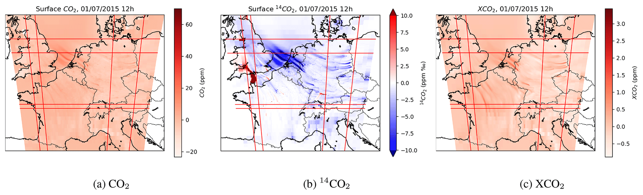
Figure 3 CO₂ (ppm) and ¹⁴CO₂ (ppm ‰) mole fractions at the surface and XCO₂ (ppm) at 12:00 UTC, on 1 July 2015: simulations from 00:00 to 12:00 UTC , without initial and boundary conditions.

2.5 Control vector

2.5.1 Definition of the control vector

The control vector is spatialized based on a decomposition of the flux maps into large or administrative regions, large urban areas, and large industrial plants.

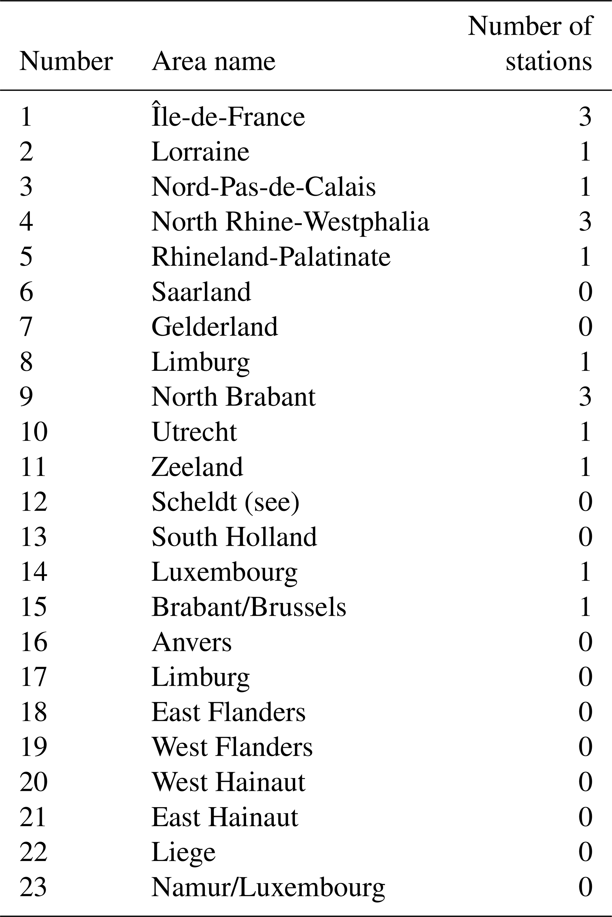
The study focuses on a set of 23 regions, called “the main area of interest” hereafter: the nine administrative regions of Belgium, Luxembourg, seven administrative regions of the southern Netherlands, three administrative regions in northern France, and three administrative regions in western Germany (all comprised in the 2 km × 2 km resolution zoom of the CHIMERE grid; see Fig. 4).

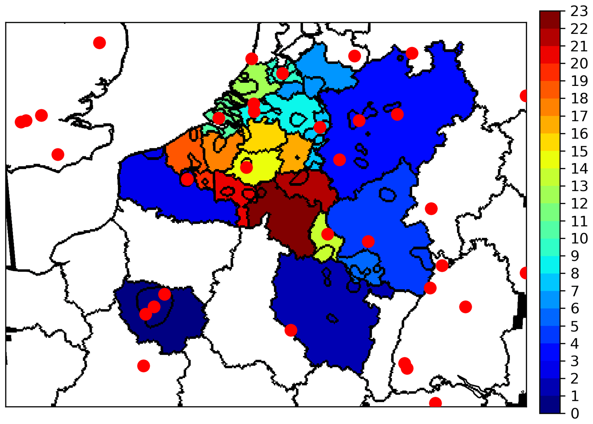
Figure 4 Main area of interest, i.e. the 23 administrative regions where major urban areas (contours of the urban areas also represented here) and point source emissions are controlled separately for anthropogenic emissions in the 2 km × 2 km resolution zoom of the CHIMERE transport model. The names of these administrative regions are listed in Table 1. Ground-based ¹⁴CO₂ and CO₂ observation sites are also shown (red dots; see Fig. 7, for the network on the whole domain).

Table 1 List of areas of control in the main area of interest and corresponding number of stations in these areas.

In this main area of interest, the CO₂ FF emission budgets from major industrial plants (22 plants for which the annual emissions exceed 1 MtC for CO₂, FF_PS; see the dots in Fig. 8a) and the FF, BF_wood, and BF_crop CO₂ emission budgets from the large urban areas (the 42 urban areas represented in Fig. 4) are controlled separately. In each of these 23 regions, the budget of the rest of the FF, BF_wood, and BF_crop CO₂ emissions is controlled separately. Outside this main area of interest, the FF, BF_wood, and BF_crop CO₂ emission budgets of 43 administrative or larger regions are controlled (Fig. 5).

Figure 5 Administrative regions and coarser areas for which the biogenic flux budgets and the anthropogenic emission budgets (with more details for regions highlighted in Fig. 4) are controlled. The red line delimits the 2 km × 2 km resolution zoom of the CHIMERE transport model.

Single ¹⁴C signatures of the BF_wood and BF_crop fluxes are controlled assuming that they apply over the whole modelling domain. The ¹⁴C fluxes from 47 nuclear power plants, across the whole modelling domain, are separately controlled.

Biogenic fluxes and isotopic signatures (NPP, HR, and δ_HR) are only controlled at the resolution of the 66 administrative regions and larger areas (23 in the main area of interest and 42 outside, Fig. 5); i.e. the spatial resolution of the control vector is nearly the same as for anthropogenic emissions, but it does not isolate urban areas and major point sources.

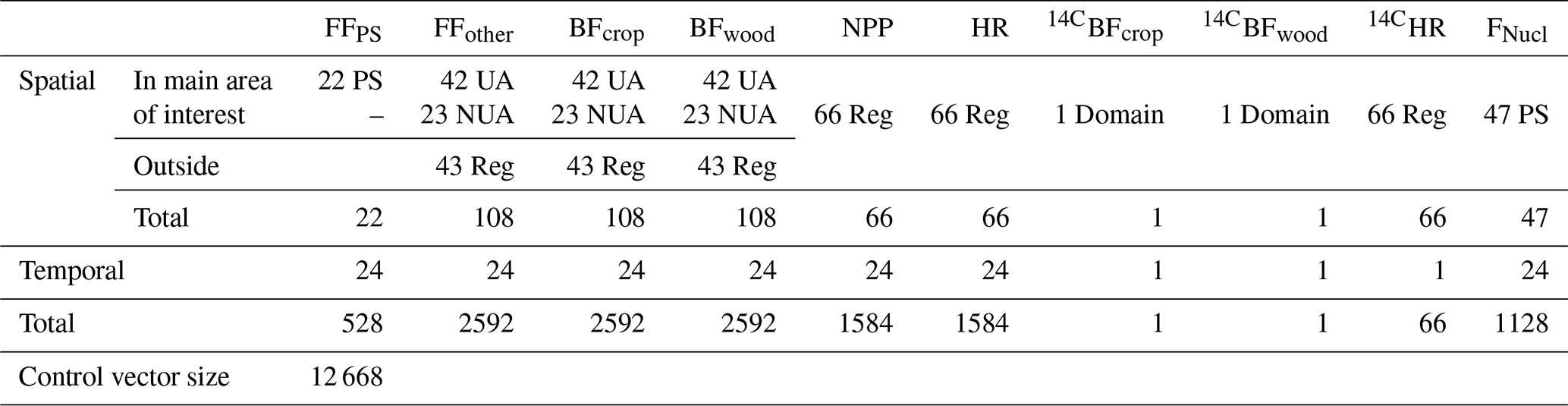
The control vector is actually composed of scaling factors to be applied to maps of local (from plant and urban area) and regional fluxes from the products presented in Sect. 2.3 over these spatial control areas at a 1 h temporal resolution except for the ¹⁴C signature of the HR, of wood burning, and of crops BF emissions which are controlled at the daily scale. Indeed, anthropogenic emissions and biogenic fluxes of CO₂ can have a high temporal variability at the hourly scale. While the product used to define the component of H_distr corresponding to nuclear emissions is based on annual values (see Sect. 2.3), the actual nuclear emissions can vary a lot at fine temporal scales (studies such as that of Cany et al., 2018, show large variations in the nuclear production of individual sites, and the emissions may actually be primarily driven by maintenance processes). The composition of the control vector is summarized in Table 2.

Table 2 Number of parameters in the control vector. The control vector is composed of scaling factors to be applied to budgets and maps of local and regional fluxes from the products presented in Sect. 2.3 (FF_PS, FF_other, BF_crop, BF_wood, NPP, HR, ^14CBF_crop, ^14CBF_wood, ^14CHR, and Nucl). This table gives number and type of areas in the control vector: 66 administrative or coarser regions (Reg) defined in Fig. 5 and more detailed areas in the main area of interest. PS: point source emissions, UA: large urban area emissions, NUA: non-urban area i.e. the rest of the region when excluding the UA and domain: whole domain budget. In a 24 h inversion window, 24 temporal parameters correspond to 1 h temporal resolution and one parameter corresponds to daily resolution.

2.5.2 Prior error covariance matrix B

B is built assuming a 3 h temporal auto-correlation of the prior uncertainty in hourly budgets for each type of controlled flux. An exponentially decaying function is used to model these temporal correlations: $e^{-d/\mathrm{3}}$, where d is the time lag, expressed in hours, between two hourly fluxes. We also assume that there is no correlation of the prior uncertainties in space (between different point sources, urban areas, and regions) or between different types of fluxes or isotopic signatures. The standard deviations of the prior uncertainties in control parameters for individual spatial areas at a daily scale are set to 30 % for FF and BF emissions, to 100 % for ¹⁴C signatures, and to 60 % for biogenic fluxes (Table 3). The resulting standard deviations of prior uncertainty in regional 24 h, morning, and afternoon budgets of FF emissions in the main area of interest range from 10 % to 45 % (Table 4). Hereafter, when analysing uncertainties in temporal budgets of fluxes, “morning” and “afternoon” are used to designate the time windows 06:00–13:00 and 13:00–19:00 UTC, respectively.

Table 3 Standard deviations of the prior uncertainties in 24 h budgets of controlled fluxes or in controlled isotopic signatures for each control area.

Table 4 Range of standard deviations of the prior uncertainty in regional 24 h, morning, and afternoon budgets of FF emissions in the main area of interest. These budgets include the urban areas and point sources within the regions

2.6 Observation vector and corresponding sets of experiments

2.6.1 Satellite observations from an XCO₂ spectral imager similar to CO2M

Some of the experiments assimilate pseudo-retrievals of XCO₂ from a single orbit of a CO2M-like satellite passing over western Europe at 12:00 UTC. The simulation of these XCO₂ satellite observations is based on the simulations of the CO2M 2 km resolution sampling, with a ∼ 300 km swath, and L2 error statistics in the surface and atmospheric conditions for the year 2014 from the ESA-PMIF project (Wang et al., 2020; Lespinas et al., 2020). These simulations account for cloud cover, which is moderate for the selected orbit (Fig. 6). The observation vector is defined by the individual cloud-free pixels of the satellite. The extraction of this observation vector from the model outputs is made by selecting the model grid cells in which the centres of these pixels are located. The spatial resolution of our transport model in the area of interest is similar to that of the satellite observation. However, since the satellite ground pixels do not perfectly correspond to the model grid cells in this area, some model grid cells can correspond to several observations. In the coarser part of the model grid, model grid cells correspond to several observations.

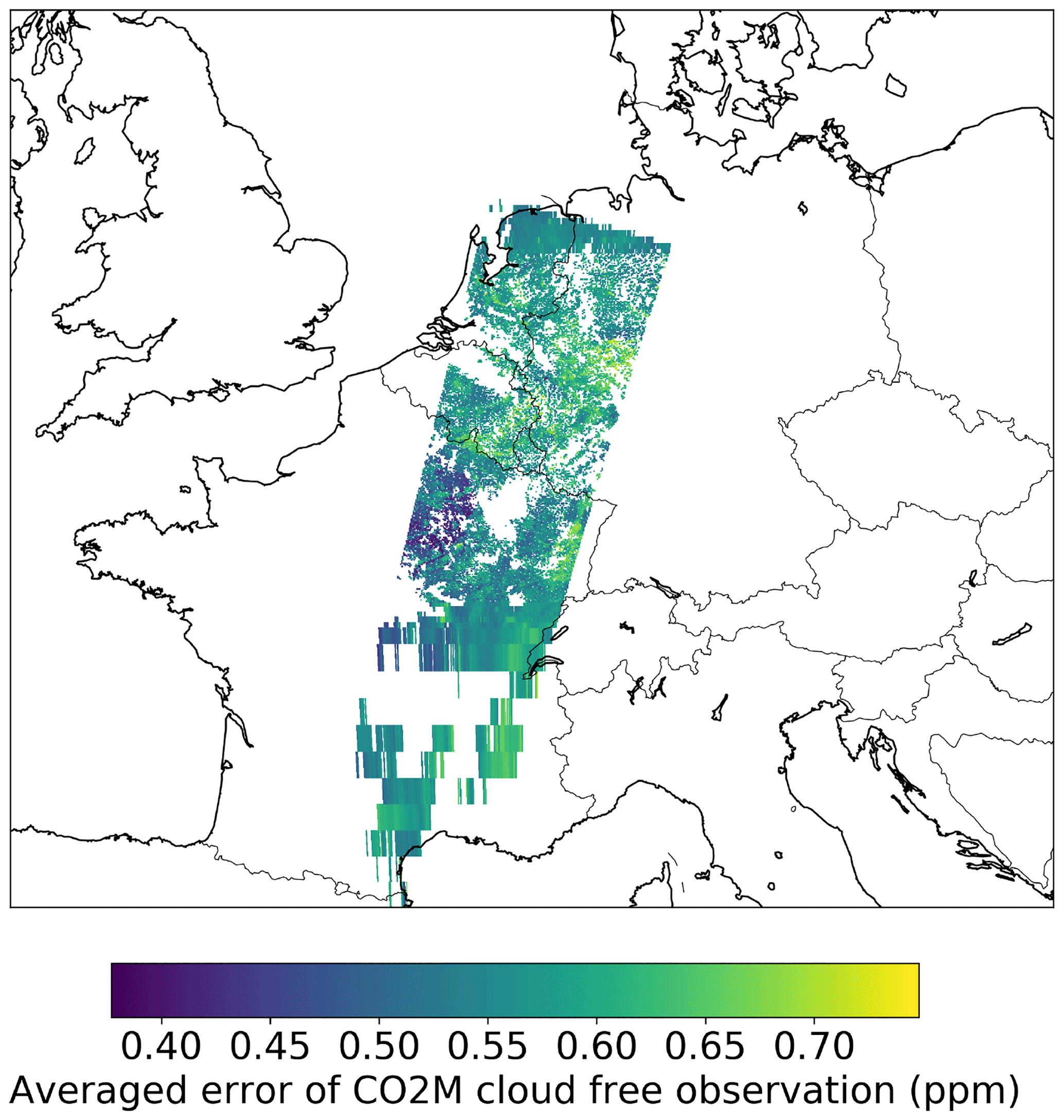
Figure 6 Simulation of the XCO₂ sampling and observation error standard deviation (by IUPB in the ESA-PMIF project) for a selected orbit of the spectral imaging satellite, in parts per million (ppm).

XCO₂ is computed from the CHIMERE 3D fields of CO₂ following the rationale of Santaren et al. (2021), notably assuming a constant vertical weighting function:

$$\begin{array}{}\text{(7)}& \begin{array}{rl}& X_{{\mathrm{CO}}_{\mathrm{2}}}(\mathrm{lat},\mathrm{lon})\\ & ={\displaystyle \frac{\stackrel{\mathrm{‾}}{{\mathrm{CO}}_{\mathrm{2}}\left(P_{\mathrm{top}}\right)}\times P_{\mathrm{top}}+{\int }_{P_{\mathrm{top}}}^{P_{\mathrm{surf}}(\mathrm{lat},\mathrm{lon})}\left({\mathrm{CO}}_{\mathrm{2}}\right(\mathrm{lat},\mathrm{lon},P)\times \mathrm{d}P)}{P_{\mathrm{surf}}(\mathrm{lat},\mathrm{lon})}},\end{array}\end{array}$$

where “lat” and “lon” are the latitude and the longitude, respectively, and P is the atmospheric pressure. P_surf is the surface pressure, and P_top (300 hPa) is the pressure at the top boundary of the model. For pressures lower than P_top, we assume that the CO₂ mole fractions equal the horizontal average of the top-level mixing ratios in CHIMERE ($\stackrel{\mathrm{‾}}{{\mathrm{CO}}_{\mathrm{2}}\left(P_{\mathrm{top}}\right)}$).

2.6.2 Ground-based network

We use a surface network (Fig. 7) of 113 stations in our modelling domain that are located following the scenario proposed by Marshall et al. (2019). This scenario is based on existing continuous CO₂ measurement sites of the Integrated Carbon Observation System (ICOS, https://www.icos-cp.eu/, last access: 25 August 2022), other air sampling stations of the National Oceanic and Atmospheric Administration (NOAA), and the Global Atmosphere Watch Programme of World Meteorological Organization (GAW, https://community.wmo.int/activity-areas/gaw, last access: 25 August 2022), but also local meteorological or air quality sampling stations and local science and engineering faculties. We assume that these stations have appropriate infrastructures and locations to observe atmospheric CO₂ and ¹⁴CO₂.

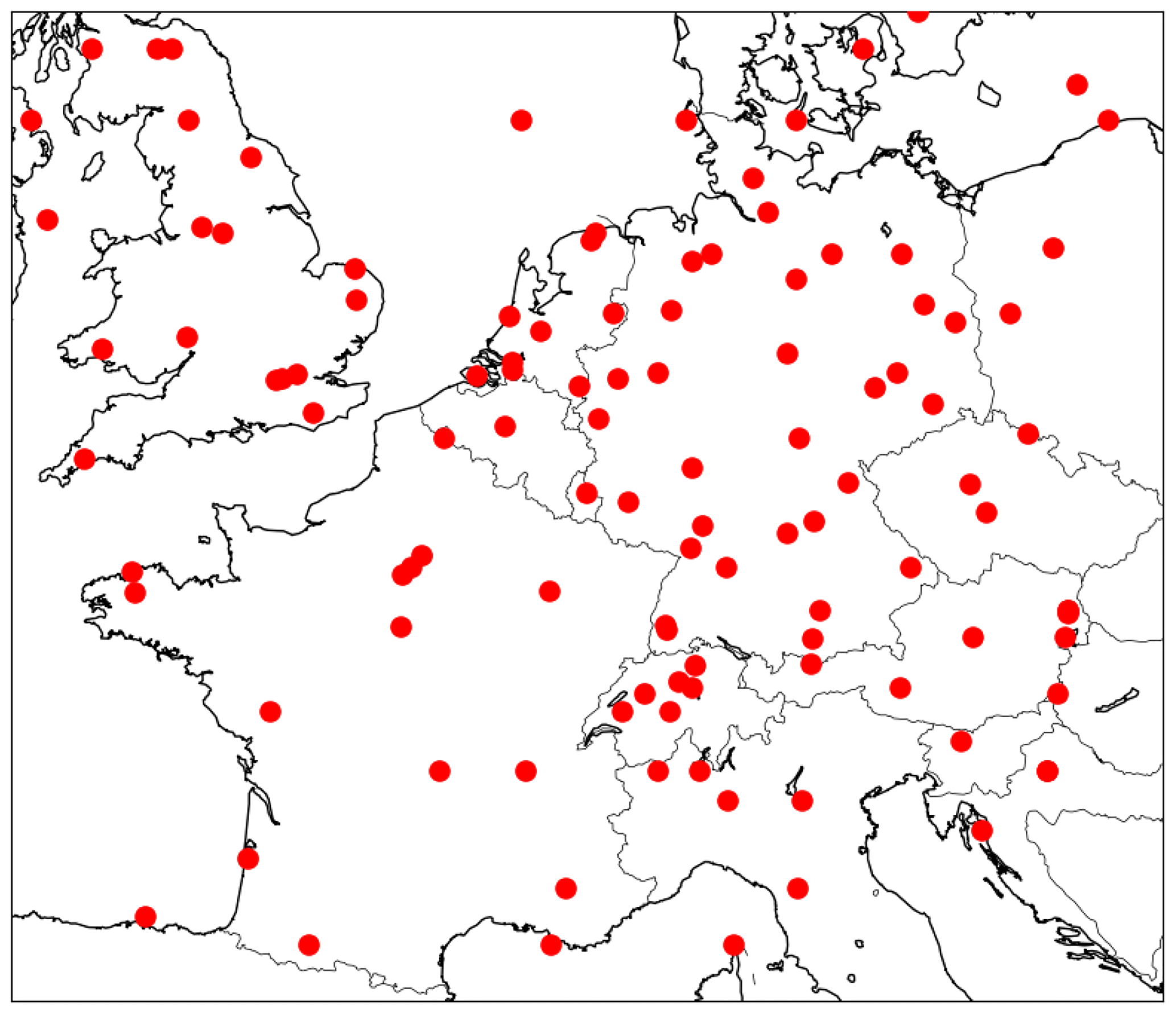
Figure 7 Ground-based ¹⁴CO₂ and CO₂ observation networks. A total of 113 stations located following the scenario proposed by Marshall et al. (2019), based on real or potential observation networks (ICOS, NOAA, GAW, more details in Sect. 2.6.2).

The sampling height at these stations ranges between 10 and 344 m above the ground level. We assume that all stations of this network simultaneously measure CO₂ and/or ¹⁴CO₂. In order to simplify the pseudo-data framework and since the main area of interest has a relatively low and flat topography, each virtual site is assumed to provide hourly CO₂ data that are suitably assimilated between 10:00 and 17:00 UTC and/or a 7 h average sample of ¹⁴CO₂ over 10:00–17:00 UTC, following the common practice of assimilating data from low-altitude stations only when the planetary boundary layer (PBL) is well developed (Broquet et al., 2011; Monteil et al., 2020; Munassar et al., 2022). The availability of CO₂ 7 h averages when deriving ¹⁴CO₂ 7 h averages from air samples is ignored.

2.6.3 Observation error covariance matrix R

The matrix R combines the uncertainty in the data that are assimilated and the corresponding uncertainty from the observation operator. Here we assume that the uncertainty in the observation operator is dominated by that of the transport model and we ignore temporal and spatial auto-correlations in these uncertainties. The representation and aggregation errors associated with the spatial and temporal resolutions of the transport model and control vector (Kaminski et al., 2001; Wang et al., 2017) are assumed to be small in the main area of interest since these resolutions are relatively high for this area in our inverse modelling framework. They are neglected over the whole domain. For individual data, the standard deviation of the observation error is therefore

$$\begin{array}{}\text{(8)}& {\mathit{\sigma }}_{\mathrm{obs}}=\sqrt{{\mathit{\sigma }}_{\mathrm{meas}}^{\mathrm{2}}+{\mathit{\sigma }}_{\mathrm{mod}}^{\mathrm{2}}}.\end{array}$$

For satellite observations, σ_meas is the uncertainty in the CO2M XCO₂ data as simulated by IUPB. These values are represented in Fig. 6. σ_mod is taken as 1 ppm for individual data (Basu et al., 2018; Marshall et al., 2019). As described in Sect. 2.6, since the satellite ground pixels do not perfectly correspond to the model grid cells, some model grid cells can correspond to several observations. We assume that the observation errors are uncorrelated: the aggregation of N observations results in decreasing errors by a factor $\mathrm{1}/\sqrt{N}$.

For the near-surface CO₂ and ¹⁴CO₂ observations, the configuration of σ_meas follows the guidelines of Marshall et al. (2019, Tables 5-1 to 5-3).

• The uncertainty in CO₂ hourly measurements is taken as the target measurement uncertainty, ${\mathit{\sigma }}_{{\mathrm{CO}}_{\mathrm{2}},\mathrm{meas}}=\mathrm{0.05}$ ppm.

• The 1σ uncertainty on ¹⁴CO₂ 7 h data is taken as 200 ppm ‰, based on the following uncertainty propagation:

  $$\begin{array}{}\text{(9)}& \begin{array}{rl}& {\mathit{\sigma }}_{{}^{\mathrm{14}}{\mathrm{CO}}_{\mathrm{2}},\mathrm{meas}}\\ & =\sqrt{{\left({\mathrm{CO}}_{\mathrm{2}}\times {\mathit{\sigma }}_{{\mathit{\delta }}^{\mathrm{14}}\mathrm{C},\mathrm{meas}}\right)}^{\mathrm{2}}+{\left({\mathit{\delta }}_{{}^{\mathrm{14}}\mathrm{C},\mathrm{a}}\times {\mathit{\sigma }}_{{\mathrm{CO}}_{\mathrm{2}},\mathrm{meas}}/\sqrt{\mathrm{7}}\right)}^{\mathrm{2}}},\end{array}\end{array}$$

  with

  • CO₂ the atmospheric mole fraction set to 400 ppm,

  • the atmospheric ${\mathit{\delta }}_{{}^{\mathrm{14}}\mathrm{C},\mathrm{a}}$ set to 40 ‰,

  • ${\mathit{\sigma }}_{{\mathrm{CO}}_{\mathrm{2}},\mathrm{meas}}/\sqrt{\mathrm{7}}$, the CO₂ measurement uncertainty at the 7 h scale, assuming that there is no autocorrelation in the CO₂ measurement errors at the hourly scale,

  • ${\mathit{\sigma }}_{{\mathit{\delta }}^{\mathrm{14}}\mathrm{C},\mathrm{meas}}=\mathrm{0.5}$ ‰ the ${\mathit{\delta }}_{{}^{\mathrm{14}}\mathrm{C}}$ measurement uncertainty at the 7 h scale.

We use the estimate of the model error from Marshall et al. (2019, Tables 5-2 and 5-3 ): ${\mathit{\sigma }}_{{\mathrm{CO}}_{\mathrm{2}},\mathrm{model}}=$1 ppm and ${\mathit{\sigma }}_{{}^{\mathrm{14}}{\mathrm{CO}}_{\mathrm{2}},\mathrm{model}}=\mathrm{1.26}\times {\mathrm{10}}^{-\mathrm{12}}$ ppm multiplied by a coefficient ranging between 1 and 5. This coefficient corresponds to the amplitude of the variability of the signal and to the level of complexity for the transport simulation at the different types of stations: 1.0 for tall towers, 1.5 for mountain sites, 3.0 for continental low-altitude stations, and 5.0 for sites within urban areas or close to strong sources. For ¹⁴CO₂, the conversion was done from ppm to ppm ‰ by multiplying by $\mathrm{1000}/R_{\mathrm{std}}$. Ignoring autocorrelations in the model error at the hourly scale, the model error for 7 h ¹⁴CO₂ mean mole fraction data is taken as $\mathrm{1}/\sqrt{\mathrm{7}}$ times the model error derived at the 1 h scale.

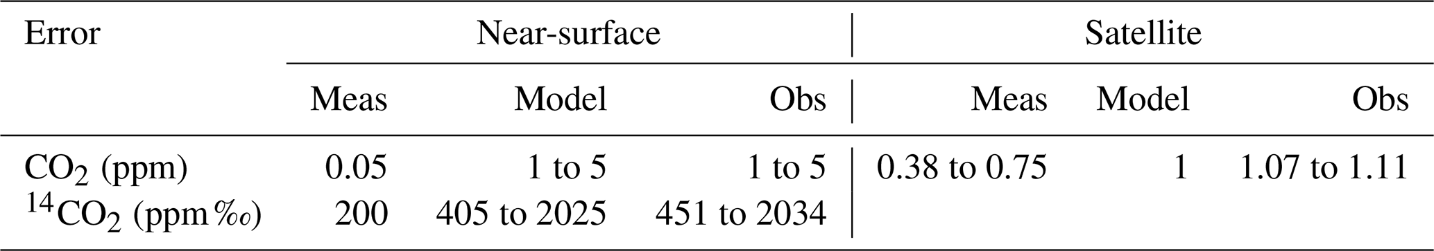
The range of the resulting error statistics on the different types of data and from the model are reported in Table 5.

Table 5 Data, model, and observation operator 1σ uncertainty.

2.6.4 List of experiments

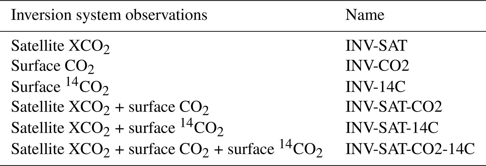
Table 6 provides labels for the different sets of experiments as a function of the sets of pseudo-observations that are assimilated, using or combining the satellite data, the surface CO₂ data, and/or the surface ¹⁴CO₂ data. The problem of the attribution of inferred fluxes to FF or BF emissions, to NEE, or to nuclear emissions is investigated by conducting sensitivity tests in which the NEE, the BF emissions, or the nuclear emissions are ignored, i.e. assuming no uncertainty in these fluxes. For the sake of simplicity, we do not define specific labels for this, and the text will clarify whenever diagnostics refer to these tests “without BF emissions, NEE, or nuclear emissions”.

Table 6 List of performed experiments.

2.7 Diagnostics

When analysing the results from the inversions and assessing the potential of the different types of observation networks, we focus on the standard deviation of the prior and posterior uncertainties in flux budgets, and on their relative difference (called uncertainty reduction or UR hereafter):

$$\begin{array}{}\text{(10)}& \mathrm{UR}=\mathrm{1}-{\displaystyle \frac{{\mathit{\sigma }}_{\mathrm{post}}}{{\mathit{\sigma }}_{\mathrm{prior}}}}.\end{array}$$

Our analyses are focused on budgets for regions in the 2 km resolution area and more particularly in the main area of interest as defined in Fig. 4.

To evaluate the impact of ground-based networks, we also define ΔUR${}_{\mathrm{Test}}^{\mathrm{Ref}}$ as the difference between UR for 24 h FF regional budgets, with a test configuration and UR with a reference configuration: ΔUR${}_{\mathrm{Test}}^{\mathrm{Ref}}$=UR_test−UR_Ref. In these cases the reference configurations are the ones when assimilating the data from the satellite track, either alone or with CO₂ data from the ground network (INV-SAT and INV-SAT-CO2; see Table 6).

3 Results

3.1 Potential of the satellite observations as a standalone observation system

This section describes results when assimilating the data from the satellite track only, i.e. results from the INV-SAT inversion.

3.1.1 General results in the morning

This section focuses on results on morning budgets for which the constraint in the inversion from the satellite observation is the highest. Indeed, the maximum UR for regional morning budgets reaches 32 % against 3 % for afternoon budgets (Table 7).

Table 7 Best score statistics of the uncertainty reductions (UR max for the highest UR) and the posterior uncertainty (Post min for the smallest posterior uncertainty) in inversions with and without NEE, for regional 24 h, morning, and afternoon FF emission regional budgets. In the main area of interest, these budgets combine emissions from urban areas, large plants, and the more diffuse regional sources.

Figure 8 shows the example of a panel of URs from INV-SAT, for the morning budget of CO₂ fluxes, at the scale of point sources to that of regions. The URs for the morning budgets of large industrial plant emissions (FF_PS) are significant in the satellite field of view (FOV, corresponding to the vertical projection of the satellite image on the ground), with values larger than 50 % (Fig. 8a), but are marginal outside this FOV. The northwest direction of the wind on the day of analysis (see Sect. 2.2) explains that the observation footprint appears to be slightly extended out of this FOV, in the east, with, for example, significant UR in the region of Essen. URs are also significant for other fossil fuel emission budgets (FF_other) and HR (heterotrophic respiration, as defined above) in the satellite FOV, with URs up to 50 % and more. The UR for NPP is much larger than for the other fluxes. This can be explained by the fact that the level of UR for a given flux is strongly driven by the ratio in the observation space between the imprint of the uncertainty in this flux and that of the uncertainty in the other fluxes added to the observation and transport model errors. The NPP is relatively large in July and thus bears a large absolute uncertainty with a widespread imprint, so that this ratio is high for this flux. The UR for BF emissions is generally much smaller than for the FF emissions. The much weaker level of emissions related to BF combustion explains the lack of UR for this type of fluxes.

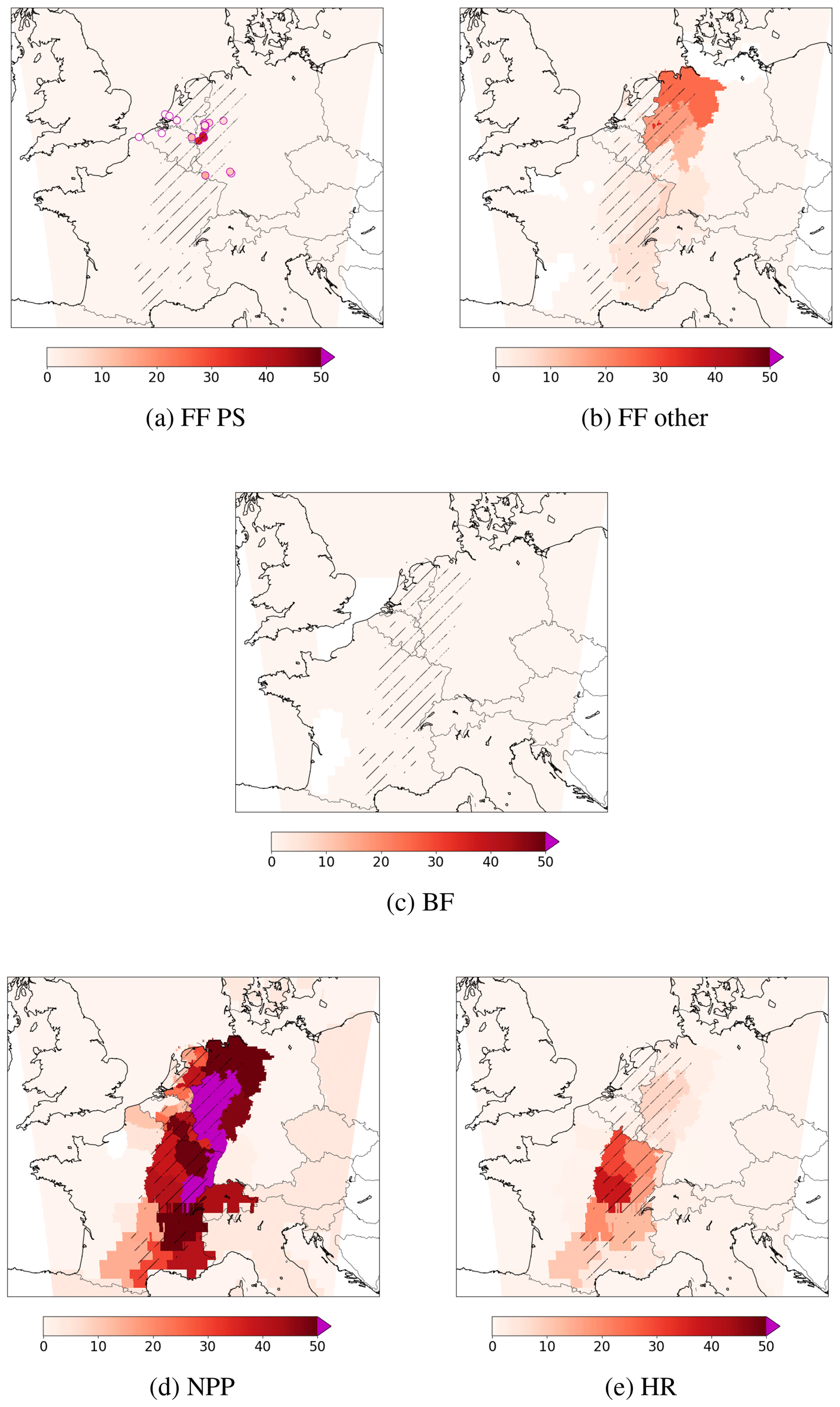
Figure 8 Uncertainty reduction in INV-Sat inversions: for morning budgets of large plants (a, FF_PS, magenta circled dots), other FF (b) and BF (c, crop and wood) emissions (urban area and rest of the region budgets), net primary production (d, NPP), and heterotrophic respiration (e, HR) (regional budgets). Stripes are indicative of the satellite field of view (see Fig. 6 for the full track).

3.1.2 Uncertainties in FF emissions

The uncertainty reductions for the 24 h regional budgets of FF emissions (regional budget aggregate emissions from urban areas, point source, and the rest of the regions hereafter) range from 0 % to 18 % in the main area of interest (Fig. 10a, Table 7). The URs are similar or rise in a range from 0 % to 32 % for the regional morning budget (Fig. 9a and Table 7). Larger emission budgets generally lead to larger URs. However, for similar or lower emission budgets (median 8 vs. 14 kTCO₂ d⁻¹, respectively), URs are significantly higher for emissions from urban areas than for the other regional emissions (max 18 % vs. 10 %, respectively) since dense emissions areas generate atmospheric signatures with large amplitudes that are easier to filter from other signatures and from the observation noise than more extended but more diffuse emissions areas (Santaren et al., 2021). URs for the afternoon emissions entirely rely on the specification of 3 h temporal auto-correlation in the prior uncertainties in the emissions since these afternoon emissions are not directly seen by the satellite in our regional inverse problem with a satellite overpass at 12:00 UTC. Consequently, URs are low for all types of sources. Figure 9b and Table 7 show URs for afternoon regional budgets ranging from 0 % to 3 %. Overall, the results show contrasting capacities for the monitoring of the FF emissions. The scores of URs result in various levels of precision on the emission estimates, with 8 % to 30 % posterior uncertainties in 24 h and regional budgets of FF emissions in the main area of interest (Table 7). The lack of constraint outside the satellite FOV and during periods other than the morning confirms the need for complementary data to extrapolate the information derived from the satellite observations in space and time.

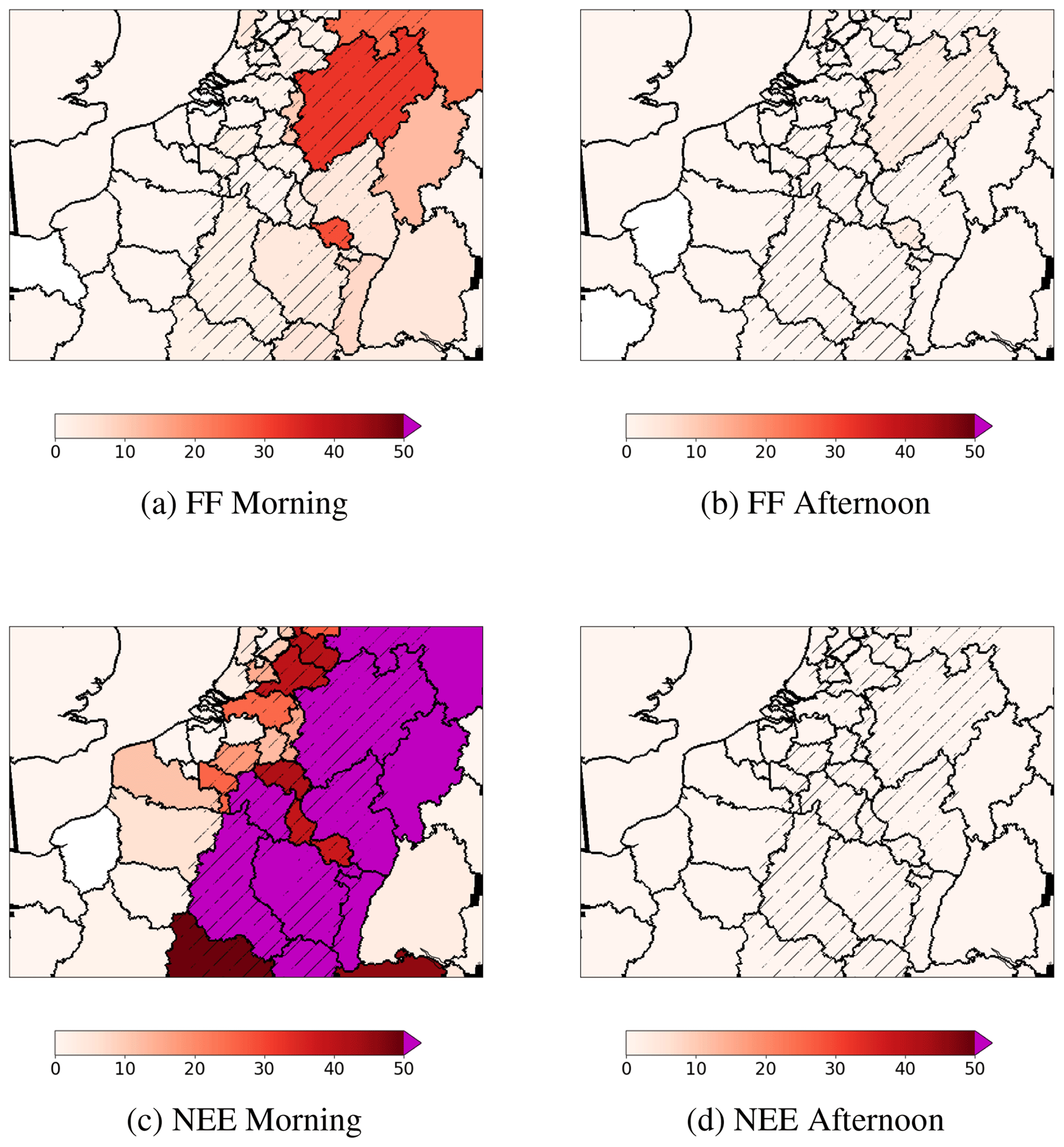
Figure 9 Uncertainty reduction in INV-Sat inversion: for morning (a, c) or afternoon (b, d) budgets of FF and biogenic fluxes (NEE). Stripes are indicative of the satellite field of view (see Fig. 6 for the full track).

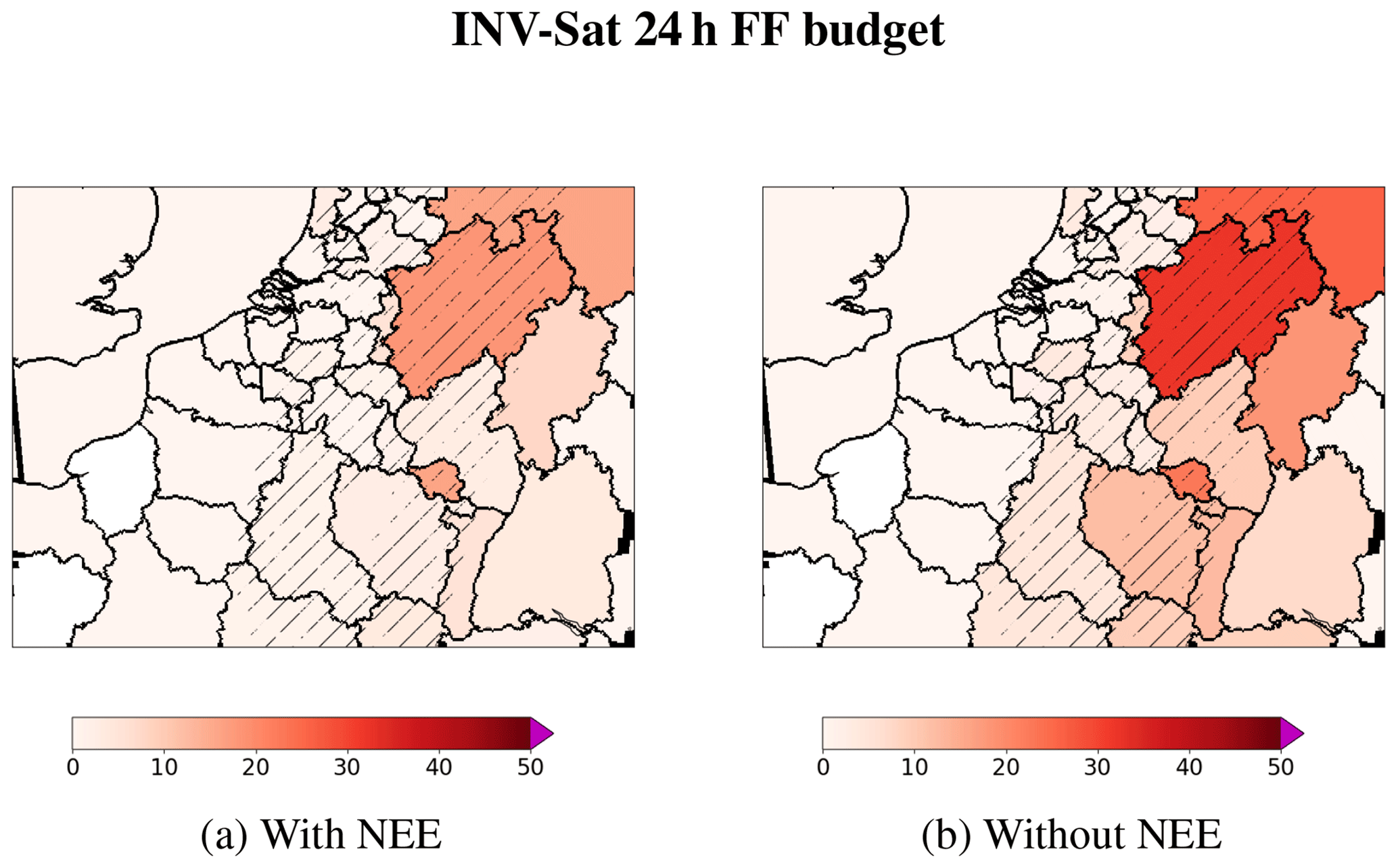
Figure 10 Uncertainty reduction in INV-Sat inversion with (a) and without (b) NEE, for 24 h budgets of FF emissions. Stripes are indicative of the satellite field of view (see Fig. 6 for the full track).

3.1.3 Impact of NEE and BF emissions on FF emissions uncertainties

The UR for NEE is much larger than for the FF emissions (Fig. 9b and c) while the UR for BF emissions is generally much smaller than for the FF emissions (Fig. 8). The problem of the attribution of inferred fluxes to FF emissions, NEE, or BF emissions is investigated with the sensitivity tests in which the NEE or BF emissions are ignored (results when ignoring BF emissions are not shown in the figures and tables for the reasons given below). The INV-SAT experiment ignoring the NEE shows significantly larger URs for the FF regional 24 h budgets (Fig. 10), up to 60 % in the satellite FOV, for the FF regional morning budget (Table 7, without NEE). This increase in the URs yields posterior uncertainties in 24 h regional budgets which can reach values as low as 6.7% in the satellite FOV (Table 7).

The sensitivity of the INV-SAT experiment to the inclusion of BF emissions shows a very weak impact of BF emissions on the UR for FF emissions (not shown) even though the spatial distribution of these two types of emissions is strongly correlated. This is directly attributed to the weak amplitude of BF emissions compared to FF emissions. Typically, the posterior uncertainty in the FF emissions (6 % to 30 % of the 24 h BF + FF emission budget) is much larger than the prior uncertainty in BF emissions (0 % to 7 % of the 24 h BF + FF emission budget).

3.2 Potential of the ground-based hourly CO₂ network

This section evaluates the impact of co-assimilating data from the ground-based hourly CO₂ network and the potential complementarity between the satellite and the CO₂ ground-based hourly observations. This evaluation is based on the analysis of INV-CO2 and INV-SAT-CO2 and comparisons with the results from INV-SAT.

3.2.1 General results for the FF emissions

INV-CO2 (Fig. 11) reveals the limited role of the horizontal atmospheric transport near the surface to propagate URs from regions with several measurement stations to other regions. URs of more than 4 %, median at 12 %, and maximum at 13 %, for 24 h budgets can be achieved in regions with three stations, like Île-de-France (Reg. 1, 12 %) and North Rhine-Westphalia (Reg. 4, 13 %) in the main area of interest (see also Fig. A1), or in regions with more stations outside this area like southeast England (10 %) and Baden-Württemberg (26 %), which have five stations. However, the UR can also be much lower in regions with many stations, e.g. for Lower Saxony and Bremen, which have five stations but a 4 % UR. UR in regions with one or two stations ranges between 0 % and 6 %. The URs are generally below 1 % for other regions. These URs reach lower or comparable values than in the INV-SAT experiment in the main area of interest (Fig. A1, Table 7). However, outside the main area of interest, Baden-Württemberg reaches a higher value than the largest one with the INV-SAT experiment (Rhineland-Palatinate, Reg. 5, 18 %).

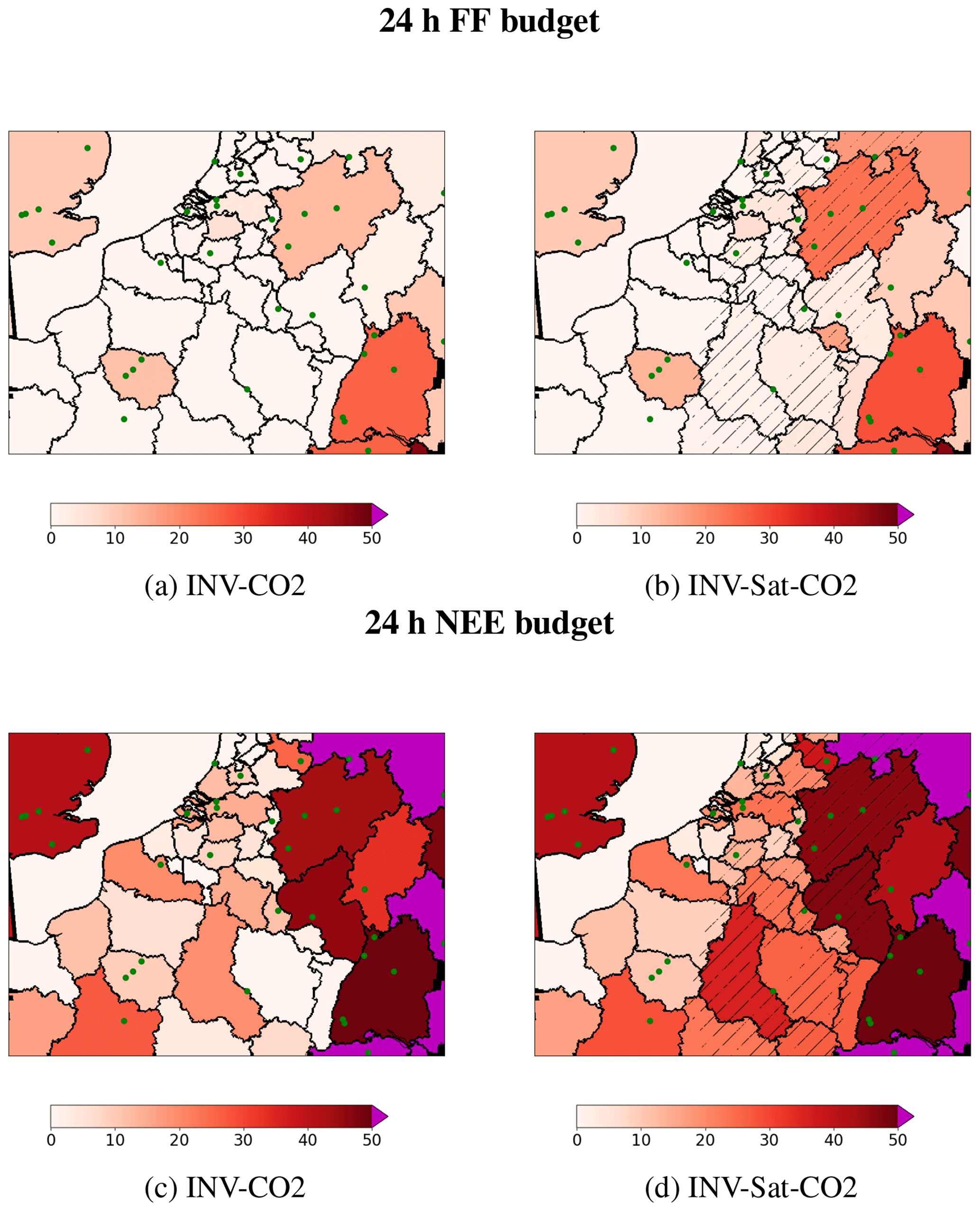
Figure 11 Uncertainty reduction in INV-CO2 (a, c) and INV-Sat-CO2 (b, d) inversions: for 24 h budgets of FF emissions and biogenic fluxes (NEE). Stripes are indicative of the satellite field of view. Green dots indicate the ground stations.

Of note is that the highest UR in the whole inversion domain (47 % for 24 h budgets and 56 % for morning budgets) corresponds to large regions of the coarse-resolution area of the transport model (not represented in Fig. 11). This result is primarily driven by the extrapolation of information from the sites to the coarse model grid cells and further to the whole extent of the control areas in which they stand, which is suitable here because of the optimistic lack of account for the representation and aggregation errors that impact observations in the coarse-resolution part of the transport and inverse modelling domains (see Sect. 2.6). This optimistic bias from the inversion configuration would actually result in representation and aggregation errors when conducting experiments with real data. The difficulty to characterize these errors (Wang et al., 2017) justifies and supports the use of the finer-resolution control vector in the main area of interest and the focus of our analysis on the 2 km resolution model subdomain. Unlike satellite data alone in INV-SAT, the ground-based CO₂ data constrain both afternoon and morning emission estimates, with URs of 4 % to 18 % and 4 % to 15 %, respectively, for morning and afternoon regional budgets of FF emissions in the regions with three or more stations (Figs. A3 and A4).

3.2.2 Co-assimilation of the satellite observations

Only one region of the 2 km resolution model subdomain with three stations is located in the satellite FOV: North Rhine-Westphalia. When comparing the URs for the 24 h regional budgets of FF emissions from INV-SAT-CO2 to that from INV-SAT and INV-CO2 (Table 8, Fig. A1) two significant changes can be seen. The first one is the decrease of 5 % in the posterior uncertainty for this region, i.e. less than the UR for this region in INV-CO2 (12 %). The second one is the increase in UR for the regions outside the satellite FOV with more than three ground-based stations from nearly 0 % to values that are nearly the same as in INV-CO2. The URs at a 24 h scale in INV-SAT-CO2 are smaller than the addition of URs in the INV-SAT and INV-CO2 experiments (Figs. 12 and A1)

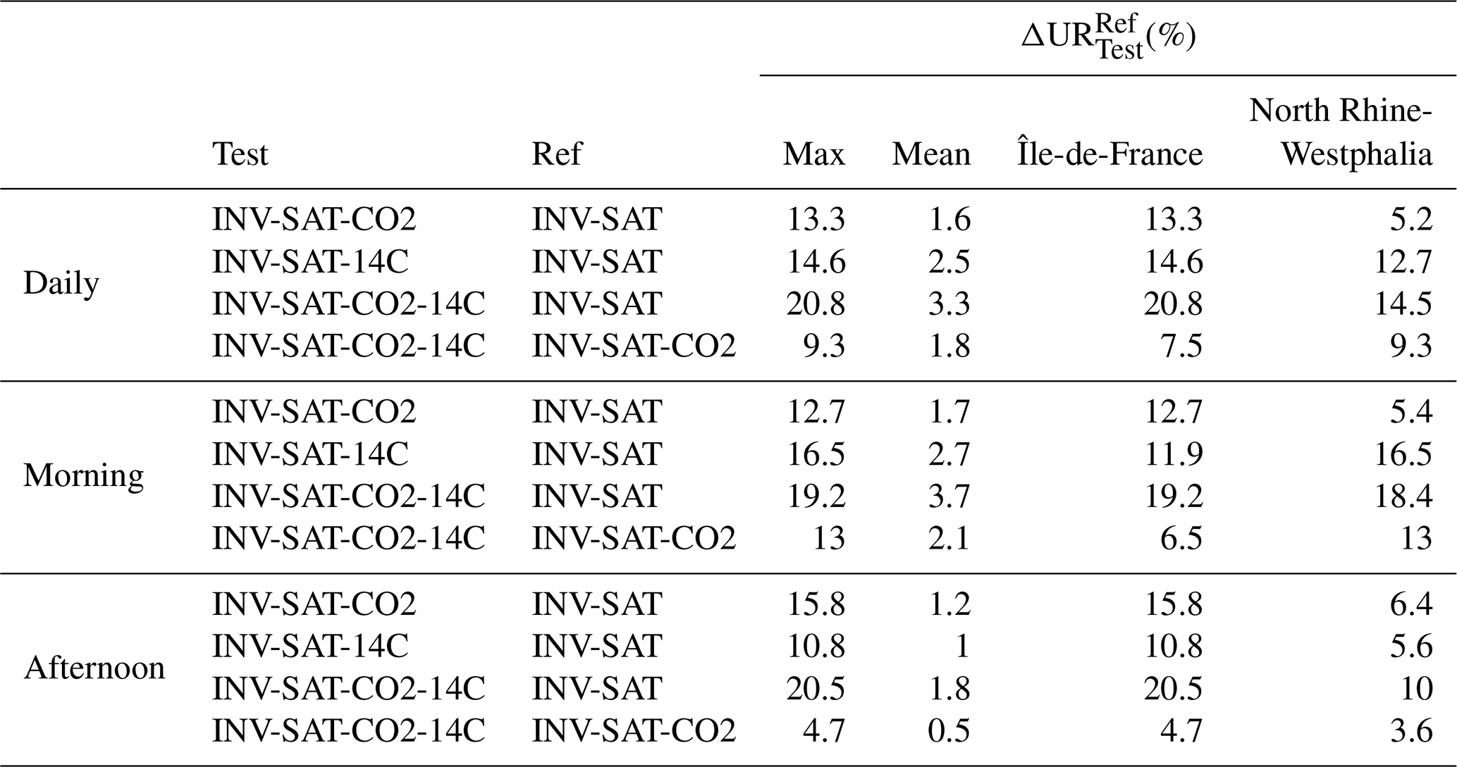
Table 8 CO₂ and/or ¹⁴CO₂ ground network impact in addition to satellite observation: ΔUR${}_{\mathrm{Test}}^{\mathrm{Ref}}$ on 24 h, morning, and afternoon FF regional budgets, maximal value on the AOI (column Max), and value of the two most impacted areas (Île-de-France and North Rhine-Westphalia columns).

The ground-based CO₂ data constrain both afternoon and morning emission estimates, with URs of 3 % to 30 % and of 1 % to 27 %, respectively, for morning and afternoon regional budgets of FF emissions in the regions with three or more stations (data not shown). The comparison between results for afternoon budgets of the FF emissions from INV-SAT-CO2 and INV-SAT shows again, in INV-SAT-CO2, an increased UR that is smaller than the sum of the URs obtained in INV-SAT and INV-CO2 (Table 7). Combining the satellite data with the afternoon data from the ground network does not increase the ability to extrapolate the spatially widely spread information from these satellite data to the afternoon.

3.2.3 Impact of NEE and BF emissions on FF emissions uncertainty

INV-CO2 and the results of INV-SAT-CO2 outside the FOV of the satellite show different situations regarding the comparison between UR for NEE and FF emissions (Fig. 11). In regions with large cities and industrial plants (like the Paris area and Baden-Württemberg), the URs for NEE are smaller than for FF as in INV-SAT. However, in other regions, the signal at the surface stations is dominated by the signature of the biogenic fluxes, and URs for NEE are larger than for FF emissions. Due to the relatively weak signal from BF emissions, the URs for these emissions are much smaller than for FF emissions (less than 3 %, less than 0.1 % on average) in INV-CO2.

The impact of the attribution problem when using the surface CO₂ network is quantified, here again, by conducting sensitivity tests in which NEE is ignored (Fig. 12 and Table 7). As the surface network has many stations mostly sensitive to the NEE signal, it is expected to support the distinction between NEE and FF emissions in the inversion, even if the stations measure CO₂ only. In inversion INV-CO2, the UR for FF emissions is higher when ignoring the NEE, reaching a range between 18 % and 46 % for 24 h budgets in the regions with more than three stations. However, the comparison between results from INV-SAT-CO2 and INV-SAT when ignoring these fluxes hardly demonstrates a potential of the surface CO₂ network to reduce the problem of attribution between FF emissions and other fluxes (Figs. 12 and 13). Figure 12 shows ΔUR${}_{\mathrm{SAT}-\mathrm{CO}\mathrm{2},\mathrm{NoNEE}}^{\mathrm{SAT}}$ larger than ΔUR${}_{\mathrm{SAT}-\mathrm{CO}\mathrm{2}}^{\mathrm{SAT}}$ on average; i.e. adding the CO₂ network when ignoring the NEE yields a larger increase in the UR than when accounting for NEE. This is linked to the smaller UR associated with CO₂ data when accounting for NEE. There is a lack of indirect feedback on the UR for FF emissions from the lowering of uncertainties in NEE when complementing the satellite data with CO₂ data.

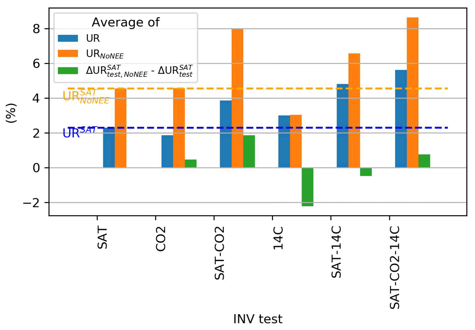
Figure 12 Average on the main area of interest of the UR on 24 h FF regional budgets in a set of inversion configurations, with (blue) and without (orange) NEE and average of the difference between ΔUR${}_{\mathrm{test}}^{\mathrm{SAT}}$ with and without NEE (green). Negative values highlight an increase in the additional observation network potential when NEE is taken into account. Positive values highlight a decrease in the additional observation network potential when NEE is taken into account. High absolute values highlight strong NEE impact.

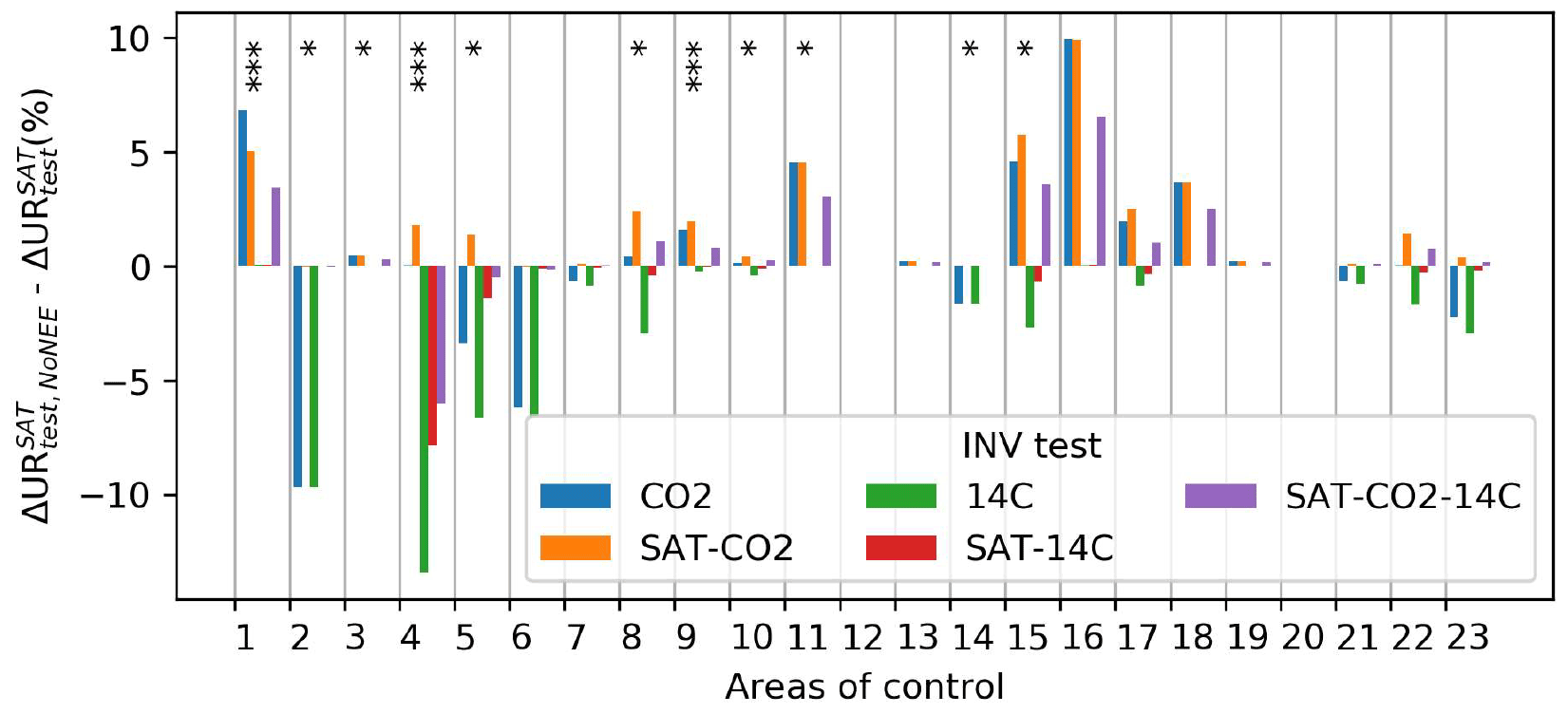
Figure 13 Impact of the NEE on the ground network capability at the top of the satellite observations for each area of control in the main area of interest: differences between ΔUR${}_{\mathrm{test}}^{\mathrm{SAT}}$ on 24 h FF regional budgets, with and without NEE. Negative values highlight an increase in the additional observation network potential when NEE is taken into account. Positive values highlight a decrease in the additional observation network potential when NEE is taken into account. High absolute values highlight strong NEE impact. The number of stars indicates the number of stations in each controlled area. The areas are listed in Table 1.

Regarding BF emissions, the results are similar to those described in Sect. 3.1, i.e. a very weak impact of BF emissions on the UR for FF emissions. With INV-SAT-CO2 the posterior uncertainties in FF emissions (7 % to 30 % of the 24 h BF + FF emission budget) are much larger than the prior uncertainty in BF emissions (0 % to 7 % of the 24 h BF + FF emission budget).

3.3 Potential of the ground-based ¹⁴CO₂ network

This section evaluates the impact of co-assimilating data from the ground-based 7 h average ¹⁴CO₂ network and the potential complementarities between the satellite and hourly CO₂ 7 h average ¹⁴CO₂ ground-based observations. This evaluation is based on the analysis of INV-14C and INV-SAT-CO2-14C and comparisons with the results from INV-CO2 and INV-SAT-CO2.

3.3.1 General results for the FF emissions

The spatial distribution of the regional URs for 24 h, morning, or afternoon budgets when using surface 7 h average ¹⁴CO₂ data alone is similar to that when using hourly CO₂ surface data only (Fig. 14). These URs are very low for regions with fewer than two stations (<7 %) and range between 12 % and 34 % for the morning budgets and between 4 % and 14 % for the afternoon budgets for regions with more than three sites. The URs on daily and morning budgets are larger in INV-14C (Table 7, Figs. A2 and A5), i.e. when using the sampling of ¹⁴CO₂ representative of 7 h averages of the mole fractions, than in INV-CO2 (Table 7, Figs. A1 and A3), when using 7-hourly CO₂ data at each site. However, the URs on afternoon budgets are smaller in INV-14C than in INV-CO2. In most regions these differences remain relatively small except in Region 4, North Rhine-Westphalia, with up to 15 percentage points in difference from the morning budget. The higher potential of ¹⁴CO₂ data (7 h averages) than hourly CO₂ data to filter the signal from FF emissions, if both were measured at the same temporal resolution, is balanced by the finer temporal resolution of the continuous hourly CO₂ measurements. The hourly CO₂ data's finer temporal resolution helps capture the high-frequency patterns of the signal from FF emissions.

Figure 14 Uncertainty reduction in INV-14C (a, c) and INV-Sat-CO2-14C (b, d) inversions: for 24 h budgets of FF emissions (a, b) and biogenic fluxes (NEE, c, d). Stripes are indicative of the satellite field of view (see Fig. 6 for the full track). Green dots indicate the ground stations.

3.3.2 Co-assimilation of the satellite and surface hourly CO₂ observations

The fact that the URs when combining two networks are smaller than the sum of the URs when using each of these networks shown when comparing INV-SAT, INV-CO2, and INV-SAT-CO2 also applies when adding the surface network, i.e. when comparing INV-SAT-14C to INV-SAT and INV-14C or INV-SAT-CO2-14C to INV-SAT-CO2 and INV-14C. The combination of 7 h average ¹⁴CO₂ data with other types of data does not lead to further synergies of the advantages for each network: the spatial extent of the satellite observation, the temporal coverage of the ground-based networks, the temporal resolution of the hourly CO₂ surface network, and the higher sensitivity to FF emissions of the 7 h average ¹⁴CO₂ network. In North Rhine-Westphalia, where the configuration is favourable, with three stations in the satellite FOV, the UR for the daily budget increases from 18 % with INV-SAT to 33 % with INV-SAT-CO2-14C (Fig. 14, Reg. 4). This configuration leads to 6.6 % posterior uncertainty. In Île-de-France (Reg. 1) outside the satellite FOV and with three stations, the UR reaches 21 % in INV-SAT-CO2-14C, reaching 18% posterior uncertainty. In Saarland (Reg. 6), in the satellite FOV and without stations, the UR remains similar in INV-SAT-CO2-14C to in INV-SAT, 17 %, corresponding to 15 % posterior uncertainty.

3.3.3 Impact of ¹⁴CO₂ sources: nuclear emissions, NEE, and BF emissions

The impact of nuclear emissions in the inversions assimilating ¹⁴CO₂ data is analysed by conducting experiments where these emissions are ignored. The comparison of INV-14C experiments with and without nuclear emissions shows a decrease in the URs, in the range of 0–1.7 percentage points (Fig. A7a), when these ¹⁴C emissions are taken into account. In the main area of interest, the most impacted areas are the Zeeland, Brabant/Brussels, Anvers, and Flanders regions where the stations are close to nuclear power plants (Fig. A7b). Outside the main area of interest, Baden-Württemberg is also strongly impacted, with up to 9 % difference.

Concerning the impact of NEE, in INV-14C, the URs for FF emissions in the regions with more than three stations are higher when ignoring the NEE, reaching a range between 15 % and 33 % for 24 h budgets. The comparison of the experiments INV-14C with and without NEE shows a much smaller impact of NEE on the URs for FF emissions than in experiments INV-CO2 or INV-SAT, which confirms the much smaller sensitivity of ¹⁴CO₂ data to NEE than CO₂ data. An interesting consequence is that, on average, ΔUR${}_{\mathrm{14}\mathrm{C}}^{\mathrm{SAT}}$, ΔUR${}_{\mathrm{SAT}-\mathrm{14}\mathrm{C}}^{\mathrm{SAT}}$ (Fig. 12), or ΔUR${}_{\mathrm{SAT}-\mathrm{CO}\mathrm{2}-\mathrm{14}\mathrm{C}}^{\mathrm{SAT}-\mathrm{CO}\mathrm{2}}$ (not shown) is slightly larger when accounting for the NEE than when ignoring them. The potential of the ¹⁴CO₂ network to complement the satellite observation is higher when NEE is accounted for, while Sect. 3.2 showed the opposite results for the surface CO₂ network. This increase in the impact of the ¹⁴CO₂ network when accounting for NEE is however relatively small, reaching its maximum in the region of North Rhine-Westphalia, which has three stations, and where the posterior uncertainty decrease for the 24 h regional budgets of FF emissions from INV-SAT to INV-SAT-14C is 15 %.

4 Discussion and conclusions

4.1 Configuration of the inversion

Several caveats should be raised for the interpretation of these results. Part of the lack of amplification of the impact from the different observation subsystems when combining them could be due to our set-up of the prior uncertainties in which we ignore spatial correlations and assume that the temporal correlations are relatively low. These assumptions are conservative and, we believe, safer, in a context where the correlations of uncertainties in current inventories are still poorly characterized and, since they are probably highly complex and far from isotropic, homogeneous, decreasing with distance or time. For instance, distant plants or cities can have more similar processes than emitters that are spatially near each other, and the emissions and their underlying processes can vary rapidly depending on the time, weather, or socio-economic drivers. Inversions assuming large temporal and spatial correlations in the prior uncertainties in inventories would indicate a stronger ability to extrapolate the information from atmospheric data but would be overly optimistic.

The control of the diffuse anthropogenic emissions and natural fluxes at the regional scale, rather than at the spatial resolution of the transport model, allowed for solving for Eq. (1) analytically, but its impact on the results could be questioned. However, the size of the control regions is quite small. Furthermore, the control of such diffuse fluxes is traditionally handled by assigning isotropic spatial correlations to the prior uncertainty in these fluxes. When considering the fluxes at high spatial resolution, this can hardly better correspond to actual errors than the partition among administrative regions, at least for the anthropogenic emissions (as highlighted above).

The study focuses on the assessment of the potential and limitation of the observation samplings, but random transport model error statistics are assigned in order to reflect the respective weight of these errors on in situ and satellite data. The specific values attributed to these statistics would directly impact the scores of posterior uncertainty and of URs. However, we assume that the ratio of transport model error statistics between the different types of observations appropriately reflects modelling skills to simulate in situ or satellite data (Marshall et al., 2019) so that the comparison of the scores of URs from the assimilation of different subsets of observations is meaningful. Furthermore, the specific values given to the error statistics, within a realistic range, should not impact the more qualitative insights brought by our analysis, regarding the spatial and temporal coverage of the information on the fluxes provided by the different types of observation networks and regarding the attribution problem.

When using real data, the actual precision of the flux estimates would be strongly impacted by atmospheric radiative transfer and transport modelling uncertainties (Schuh et al., 2019; Crowell et al., 2019). Our model of the uncertainty in the atmospheric transport is relatively simple here: a Gaussian distribution without any spatial and temporal correlation in the observation space of the inversion problem, as traditionally done in atmospheric inversions (Peiro et al., 2022; Crowell et al., 2019). Complex modelling errors could actually shift or modify the patterns of the atmospheric signature of the FF emissions, which could increase the weight of the attribution problem and thus the potential of the combination between satellite and surface data. However, very dense surface networks would be needed to support the identification and adjustment of transport errors. Uncertainties in the radiative transfer inverse modelling, which underlies the retrieval of XCO₂, yield systematic errors in the XCO₂ data, i.e. errors with spatial correlations. These errors are a major component of the observation errors. Their impact on the inversions highly depends on their structure and on the ability, in the inversion systems, to anticipate for such a complex error component (Santaren et al., 2021). We deliberately avoided accounting for such error components resulting from numerical models because they can hardly be characterized appropriately by the type of OSSEs conducted here and because they consist in unknown time-evolving residuals, for which existing studies hardly provide more than qualitative insights or case-specific values. They tend to diminish along with model and remote sensing progress, in contrast to random errors, which explains the focus of this study on the potential and limitation of the observation systems.

Other types of errors may have been ignored in our inversion configuration while potentially having a significant impact. Our reasoning pushed for neglecting the uncertainty in the large- and fine-scale patterns of the initial and boundary conditions. Santaren et al. (2021) showed a low impact of uncertainties in a single scaling factor for the whole initial and boundary conditions of the modelling window and domain at the 6 h scale, and the fine-scale patterns are assumed to vanish quickly in time. However uncertainties in the gradients along the boundaries and in synoptic patterns might actually have a large amplitude which persists across the modelling domain and perturbs the identification of atmospheric imprints of the local and regional fluxes. Results have shown that the representation and aggregation errors should be accounted for at the ground observation stations outside the main area of interest, where the spatial transport and inversion resolutions are coarse. These errors might also need to be re-assessed in the high-resolution part of the domain, but Bréon et al. (2015) used similar transport and control resolutions, and they showed that there errors should be low, even at stations at the edge of urban areas. In a more general way, the quantitative results from our experiments, like those from all OSSEs, can suffer from the lack of account for specific sources of errors or for the lack of ability to properly characterize complex ones. However, they support a good understanding of the inversion processes and of the potential of the observation networks.

The use of XCO₂ sampling and error simulations for a day in 2014 while the flux and transport modelling framework corresponds to another day in 2015 raises an inconsistency between the cloud patterns and the meteorological forcing of the atmospheric transport. However, the cloud cover in the selected satellite track is moderate, the gaps due to this cover are spread relatively homogeneously along the track, and a redistribution of these gaps with similar fraction of cloudy scenes should not impact the general results. Similarly, the potential inconsistency between the variations in space of the XCO₂ errors (which are limited, in the range 0.4 to 0.7 ppm) and the atmospheric conditions is assumed to be negligible.

The results, in particular those of the sensitivity tests with and without NEE or nuclear emissions, demonstrate the need for a complex simulation of the CO₂ and ¹⁴CO₂ transport, taking into account the diversity of ¹⁴CO₂ sources and sinks, and are more realistic than the common simplification which consists of representing only the dilution of radiocarbon-free FF CO₂ emissions. This and an inversion system at high resolution are more suitable for assessing the real ability to extrapolate information from the ¹⁴CO₂ atmospheric data. However, given its high spatial and temporal resolution, the analytical inversion framework used here can hardly be run over several days, because the size of the matrices to be inverted would become too large. Therefore, inversions have been run for 1 d only, on 1 July 2015, i.e. for very specific atmospheric conditions and biogenic fluxes. In summer the biogenic fluxes are relatively high. Tests over different days, e.g. in winter, could bring a more precise characterization of the complementarity of in situ networks with satellite data, but the primary focus of this study was to investigate the problem of the separation between the biogenic fluxes and FF emissions. By limiting the inversion window to a single day, we avoid analysing to which extent the temporal correlations of the uncertainties in the FF CO₂ emission inventories allow for cross-referencing the information of data from different days. This assessment should rely on a strong knowledge on the structures of uncertainties in the FF emissions, which is still incomplete, as illustrated above, even though efforts have been conducted to improve this issue (Wang et al., 2020; Super et al., 2020).

Finally our study tested a surface network roughly corresponding to the extension of a continental network like ICOS for the monitoring of regional FF emission budgets. The deployment of networks dedicated to specific cities with stations around and within the urban areas (Wu et al., 2016) would correspond to a different strategy and could result in different conclusions for the monitoring of city emissions.

4.2 Insights from the results

The results presented here raise contrasting conclusions regarding the potential of the combination between the satellite observation and the surface networks. The satellite observation, as a stand-alone system, can yield estimates of the regional budgets of FF emissions in the morning corresponding to its days of overpass with uncertainties down to 10 % (prior 15 %, UR 32 %) in its FOV. However, it does not provide direct information on emissions during the afternoon or during the night, and it hardly provides information on plants, cities, and regions outside its FOV. Furthermore, previous publications (Broquet et al., 2018; Wang et al., 2020; Lespinas et al., 2020; Kuhlmann et al., 2019) have shown that, even with a CO2M constellation of three or more satellites, the number of overpasses producing local images with low cloud cover is limited each year. The data gaps are not random over time and hamper the estimation of annual budgets or their anomalies, as illustrated in the case of the “great lockdown” (Chevallier et al., 2020). The need for complementary sources of information to derive daily to annual budgets is thus critical.

The problem of attributing the inferred CO₂ fluxes to specific emission and absorption types appears to be nearly secondary compared to that of the satellite observation precision, but our results confirm that there is a significant impact of the uncertainty in the NEE for the estimate of FF emissions. The uncertainty in BF emissions does not appear to have a large impact on the estimate of FF emissions, but this is related to the fact that the posterior uncertainty in FF emissions remains larger than the prior uncertainty in BF emissions, i.e. to the relatively low level of BF emissions compared to the typical uncertainties in FF emissions at regional to local scales. If the goal is to achieve higher-precision estimates of the FF emissions than those obtained with the present configuration, for example with higher-precision spaceborne instruments, and if the share of BF emissions increases in the future, the uncertainty in BF emissions would probably become a major problem due to the strong correlation between the spatial distributions of FF and BF emissions. The problem of attribution to NEE fluxes would also increase with this goal of higher-precision estimates of the FF emissions in the future.

Surface ${\mathrm{CO}}_{\mathrm{2}}{/}^{\mathrm{14}}{\mathrm{CO}}_{\mathrm{2}}$ networks can help further decrease the uncertainty in the FF emissions estimates when combined with satellite observations. In North Rhine-Westphalia, the addition of CO₂ and ¹⁴CO₂ stations decreases the posterior uncertainty in daily regional emissions from 8 % with the satellite alone to 6.6 %. However, relatively dense networks close to highly emitting areas are needed to support such a decrease. The isolated stations far from the urban areas do not provide a direct strong constraint for the estimate of the FF emissions nor a significant indirect constraint for this estimate by solving for the attribution problem. Our results suggest that surface CO₂ and/or ¹⁴CO₂ measurements in support of the FF emission monitoring should be targeting FF emission areas directly and located close to these areas rather than in the more remote countryside dominated by signals from the NEE. Both hourly CO₂ and daily ¹⁴CO₂ data can provide useful information on the FF emissions, the former catching the signature of these emissions at high frequency and the latter being much less sensitive to the uncertainty in the NEE.

Overall, the results illustrate a decrease in the potential of each observation subsystem rather than an amplification of these potentials when combining them together into a large observation system with satellite and surface data. This is the natural consequence of the asymptotic convergence of the precision of inversions towards some low value when adding observations. In our experiments, crossing the spatial extent of the satellite observation, the temporal coverage (with observations between 10:00 and 17:00 UTC and a wider temporal representativity) of the ground-based networks, the temporal resolution (hourly) of the CO₂ surface network, and the higher sensitivity to FF emissions of the ¹⁴CO₂ network do not lead to the expected synergy with wide spatio-temporal coverage of the FF emissions at high resolution. There is a lack of new extrapolation of information from the combination of observation subsystems. This may be due to the specificities of the attribution and extrapolation problems in our inversion case.

Therefore, these results support the deployment of very dense CO₂–¹⁴CO₂ surface networks to support the satellite observation, with at least three sites per European administrative region. The large-scale deployment of such dense networks is probably unaffordable in the coming decade, but some regions are now equipped with many stations, and in some locations, the complementarity between satellite and surface networks could thus be demonstrated. Frequent (up to daily) samplings of ¹⁴CO₂ would be needed to ensure ¹⁴CO₂ data can bring information on FF emissions more precise than that of hourly CO₂ measurements.

Appendix A

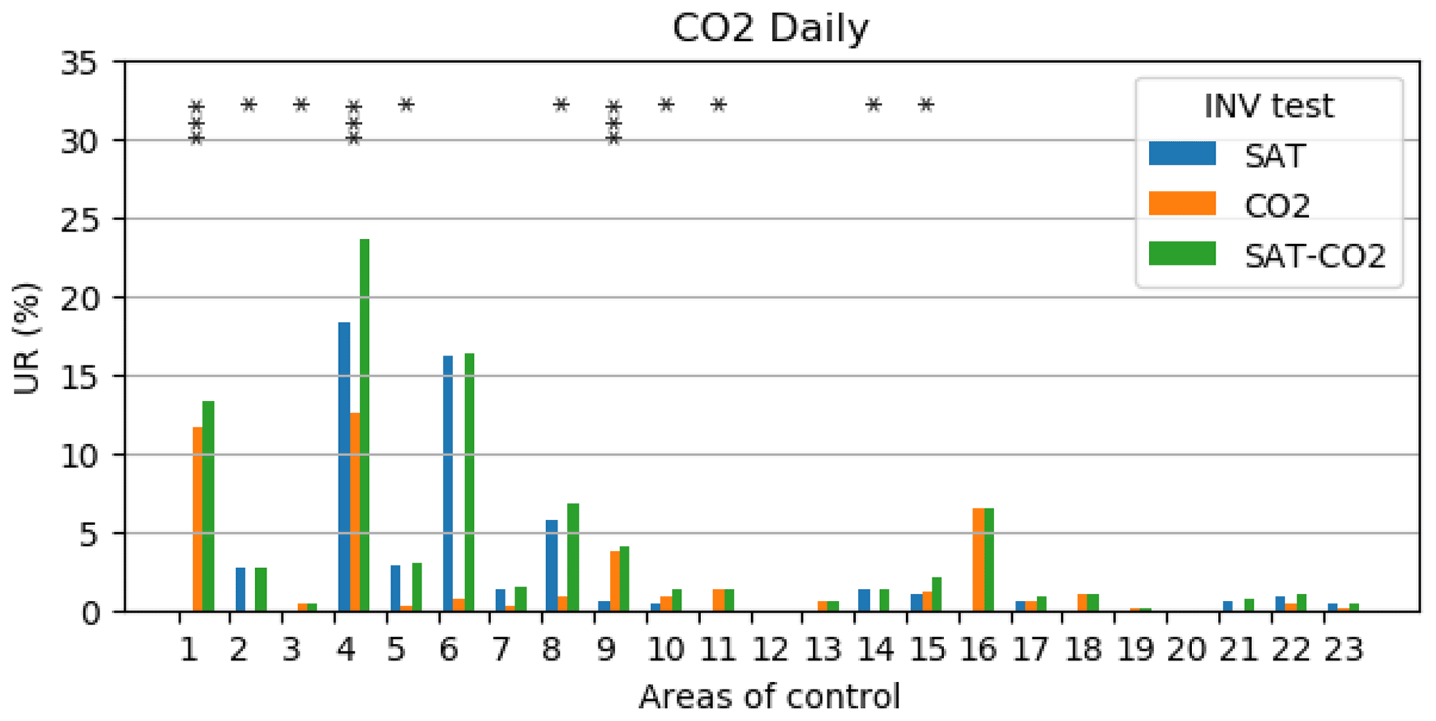
Figure A1 Uncertainty reduction in INV-SAT, INV-CO2, and INV-SAT-CO2 inversions for 24 h budgets of FF emissions of each controlled area in the main area of interest. The number of stars indicates the number of stations in each controlled area. The areas are listed in Table 1.

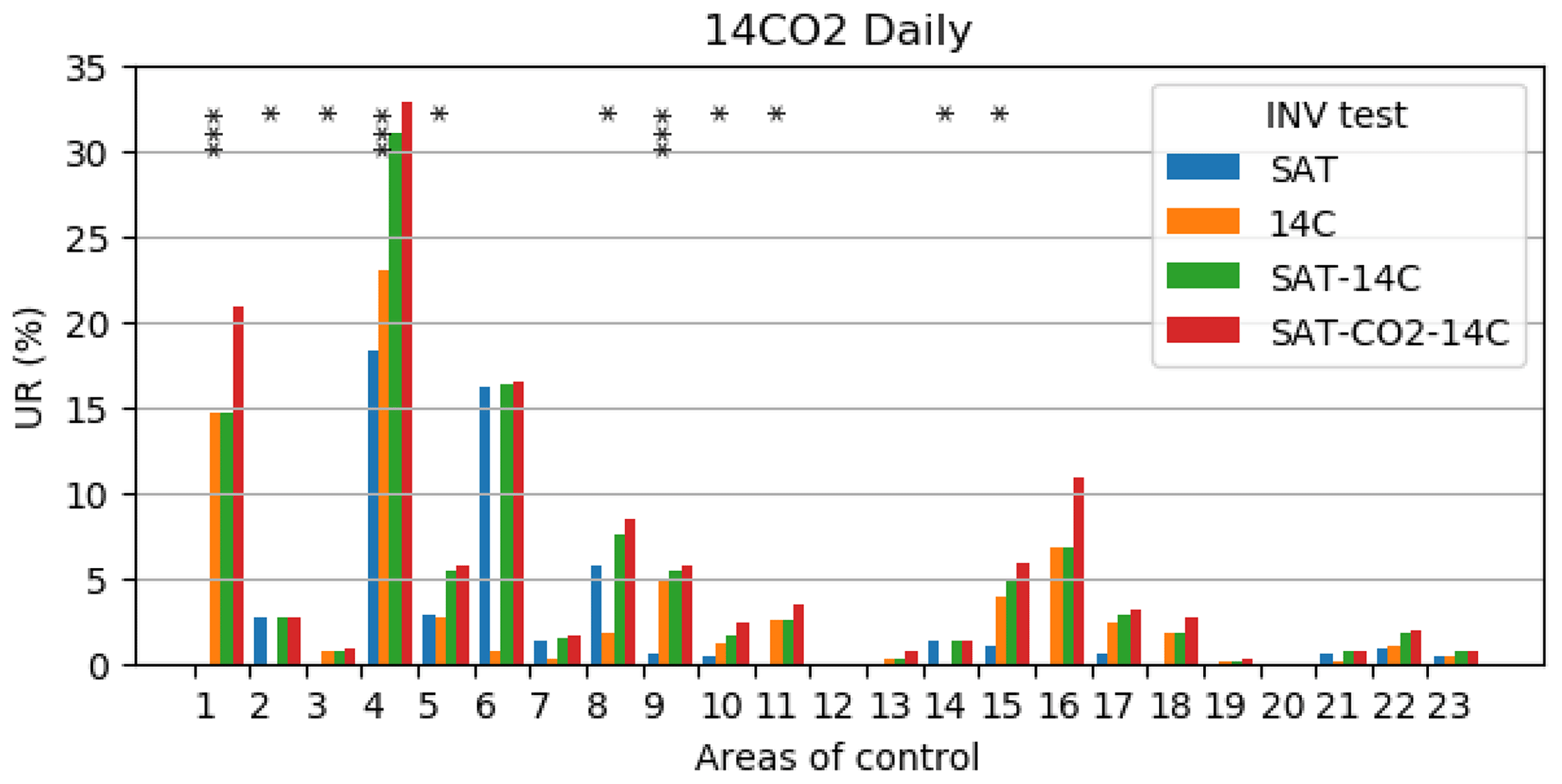
Figure A2 Uncertainty reduction in INV-SAT, INV-14C, INV-SAT-14C, and INV-SAT-CO2-14C inversions for 24 h budgets of FF emissions of each controlled area in the main area of interest. The number of stars indicates the number of stations in each controlled area. The areas are listed in Table 1.

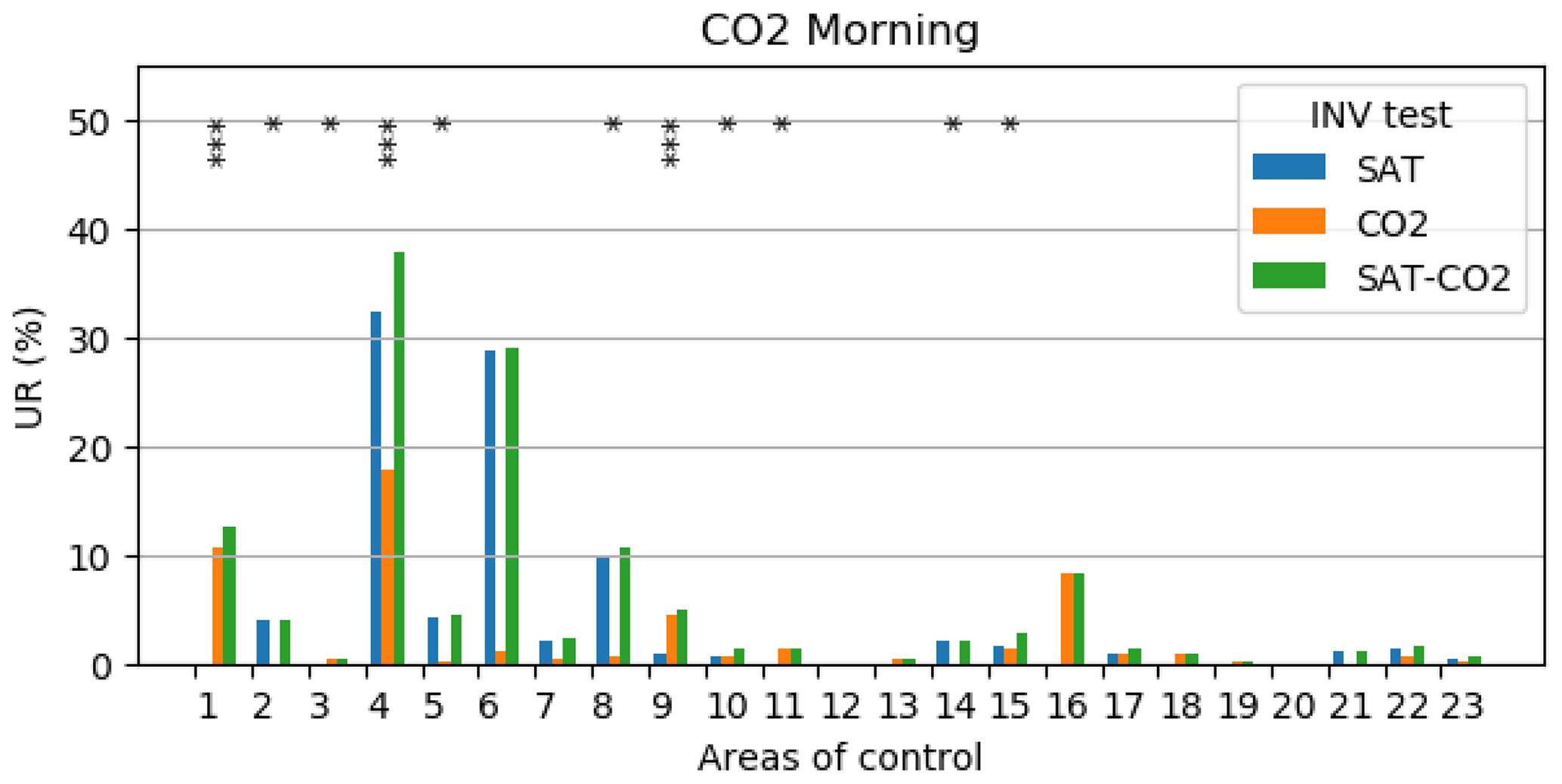
Figure A3 Uncertainty reduction in INV-SAT, INV-CO2, and INV-SAT-CO2 inversions for morning budgets of FF emissions of each controlled area in the main area of interest. The number of stars indicates the number of stations in each controlled area. The controlled areas are listed in Table 1.

Figure A4 Uncertainty reduction in INV-SAT, INV-CO2, and INV-SAT-CO2 inversions for afternoon budgets of FF emissions of each controlled area in the main area of interest. The number of stars indicates the number of stations in each controlled area. The names of the controlled areas are listed in Table 1.

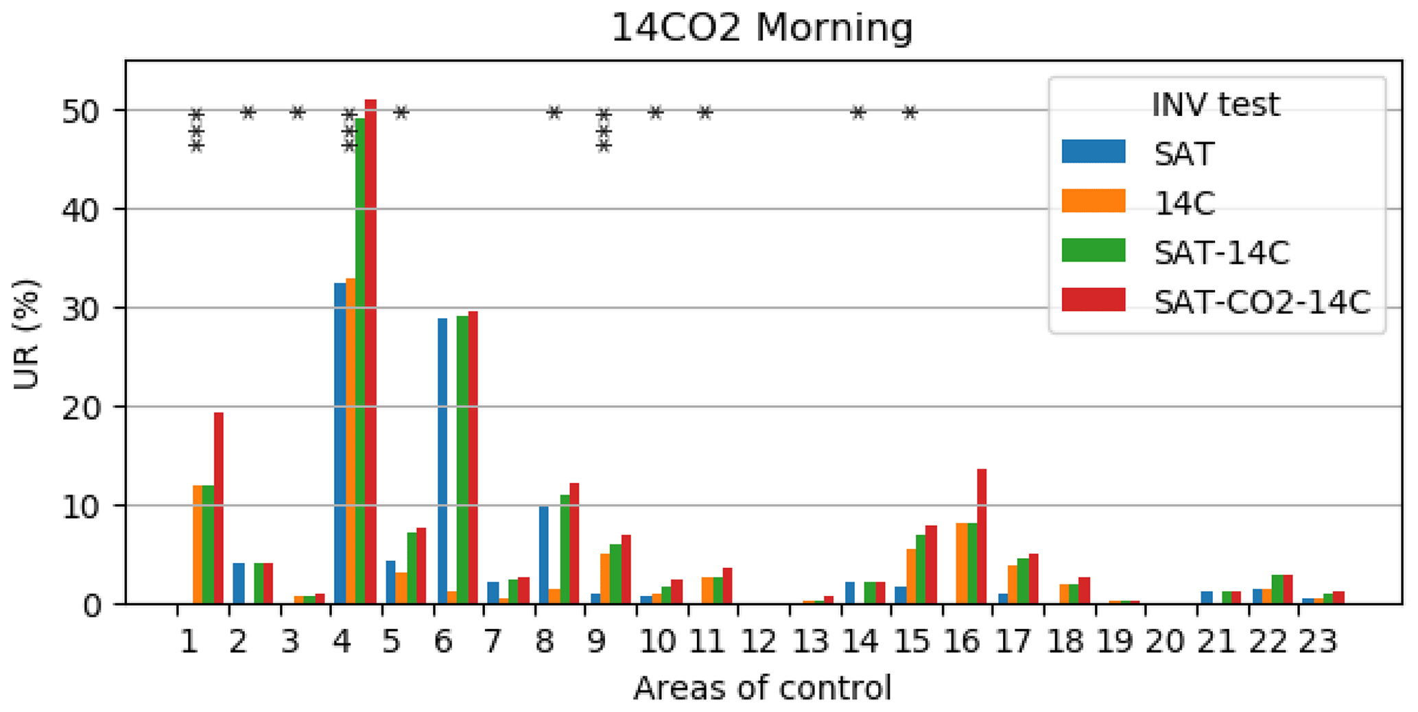
Figure A5 Uncertainty reduction in INV-SAT, INV-14C, INV-SAT-14C, and INV-SAT-CO2-14C inversions for morning budgets of FF emissions of each controlled area in the main area of interest. The number of stars indicates the number of stations in each controlled area. The names of the controlled areas are listed in Table 1.

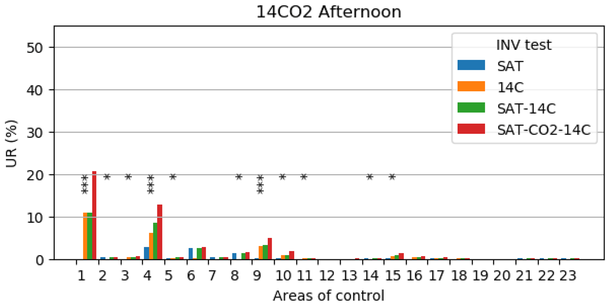
Figure A6 Uncertainty reduction in INV-SAT, INV-14C, INV-SAT-14C, and INV-SAT-CO2-14C inversions for afternoon budgets of FF emissions of each controlled area in the main area of interest. The number of stars indicates the number of stations in each controlled area. The names of the controlled areas are listed in Table 1.

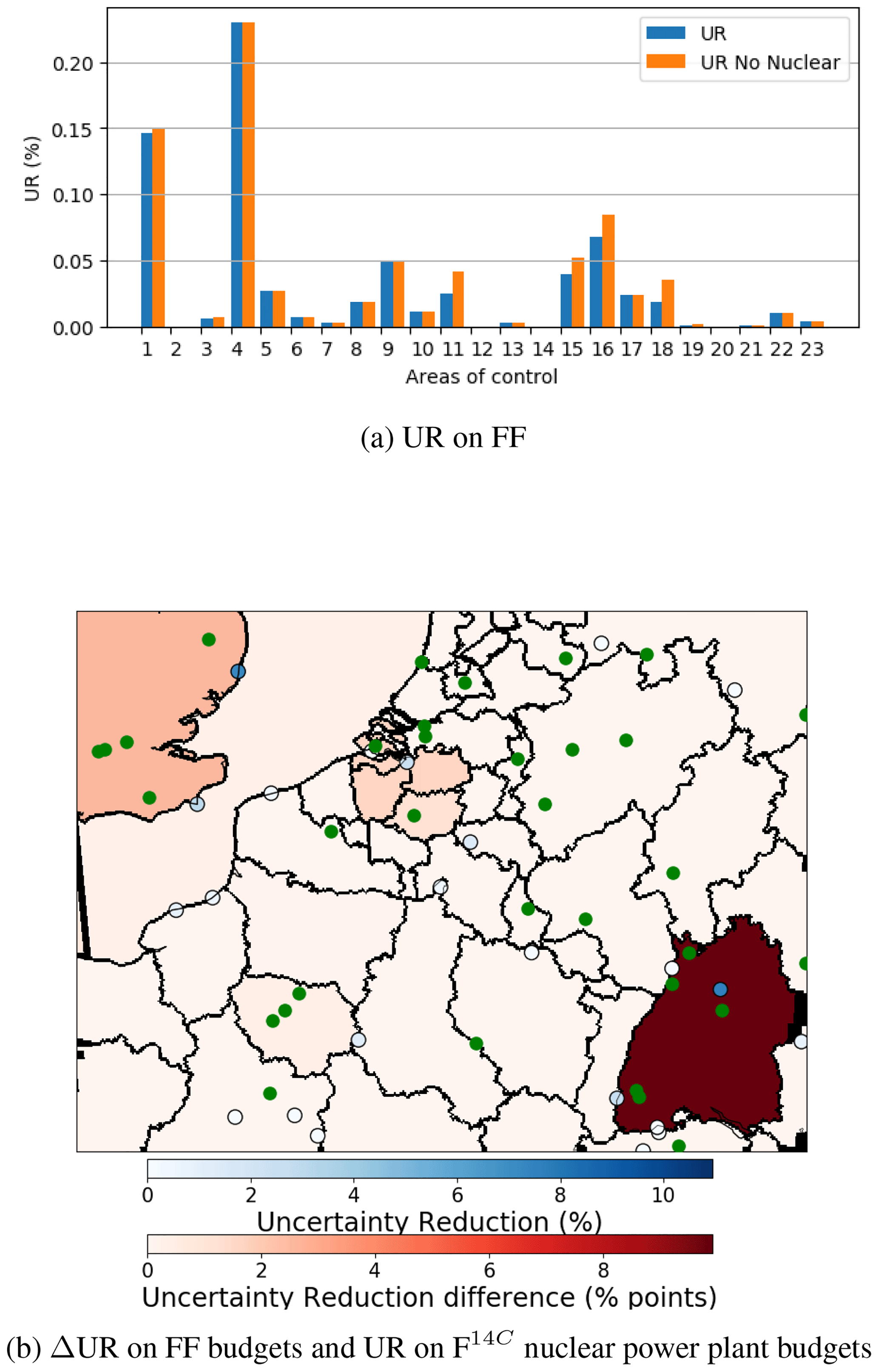
Figure A7 (a) Uncertainty reductions, on 24 h FF budgets, with and without nuclear emissions in INV-14C inversion, for each controlled area in the main area of interest. The names of the controlled areas are listed in Table 1. (b) Maps of the 2 km resolution area of the differences between uncertainty reductions with and without nuclear emissions (shades of red) in INV-14C inversions and uncertainty reductions on $F^{{}^{\mathrm{14}}\mathrm{C}}$ nuclear power plant budgets (F_Nucl in the main text) (dots, shades of blue). Green dots indicate the ground stations.