Extended validation and evaluation of the OLCI–SLSTR SYNERGY aerosol product (SY_2_AOD) on Sentinel-3

We present the first extended validation of a new SYNERGY global aerosol product (SY_2_AOD), which is based on synergistic use of data from the Ocean and Land Color Instrument (OLCI) and the Sea and Land Surface Temperature Radiometer (SLSTR) sensors aboard the Copernicus Sentinel-3A (S3A) and Sentinel-3B (S3B) satellites. Validation covers period from 14 January 2020 to 30 September 2021. Several approaches, including statistical analysis, time series analysis, and comparison with similar aerosol products from the other spaceborne sensor, the Moderate Resolution Imaging Spectroradiometer (MODIS), were applied for validation and evaluation of S3A and S3B SY_2 aerosol products, including aerosol optical depth (AOD) provided at different wavelengths, AOD pixel-level uncertainties, fine-mode AOD, and Angström exponent.

Over ocean, the performance of SY_2 AOD (syAOD) retrieved at 550 nm is good: for S3A and S3B, Pearson correlation coefficients with the Maritime Aerosol Network (MAN) component of the AErosol RObotic NETwork (AERONET) are 0.88 and 0.85, respectively; 88.6 % and 89.5 % of pixels fit into the MODIS error envelope (EE) of ±0.05 ± 0.2 × AOD.

Over land, correlation coefficients with AERONET AOD (aAOD) are 0.60 and 0.63 for S3A and S3B, respectively; 51.4 % and 57.9 % of pixels fit into MODIS EE. Reduced performance over land is expected since the surface reflectance and angular distribution of scattering are higher and more difficult to predict over land than over ocean. The results are affected by a large number of outliers.

Evaluation of the per-retrieval uncertainty with the χ2 test indicates that syAOD prognostic uncertainties (PU) are slightly underestimated (χ2 = 3.1); if outliers are removed, PU describes the syAOD error well (χ2 = 1.6).

The regional analysis of the Angström exponent, which relates to the aerosol size distribution, shows spatial correlation with expected sources. For 40 % of the matchups with AERONET in the Northern Hemisphere (NH) and for 60 % of the matchups in the Southern Hemisphere (SH), which fit into the AE size range of [1, 1.8], an offset between SY_2 AE (syAE) and AERONET AE (aAE) is within ±0.25. General overestimation of low (< 0.5) syAE and underestimation of high (> 1.8) syAE results in high (0.94, globally) overall bias.

Good agreement (bias < 0.03) was observed between Sy_2 fine-mode AOD (syFMAOD) and AERONET fine-mode AOD (aFMAOD) for aFMAOD < 1. At aFMAOD > 1, syFMAOD is considerably underestimated (by 0.3–0.5 in different aFMAOD ranges) in the NH. In the SH, only a few aFMAOD values above 1 are measured. The fine-mode fraction (FMF) in the SY_2 AOD product (syFMF) in the range of [0, 0.7] is overestimated; the positive offset of 0.3–0.5 for low (< 0.25) FMF gradually decreases.

Differences between the annual and seasonal AOD values from SY_2 and MODIS (mod) Dark Target and Deep Blue products are within 0.02 for the study area (30^∘ S–60^∘ N, 80^∘ W–45^∘ E). The agreement is better over ocean; however, a difference up to 0.6 exists between syFMF and modFMF. Over bright land surface (Saharan desert) the difference in AOD between the two products is highest (up to 0.11); the sign of the difference varies over time and space.

For both S3A and S3B AOD products, validation statistics are often slightly better in the Southern Hemisphere. In general, the performance of S3B is slightly better.

1 Introduction

The concern about climate change (e.g. Bergquist and Warshaw, 2019) along with a willingness to reduce its effects (e.g. Leiserowitz et al., 2020; Hoffmann et al., 2022) have been of growing interest during the past decades. Global models introduce different scenarios for climate change (Arbor et al., 2021; Meehl et al., 2007), which are often based on the historical records and trends. Satellite data, including aerosols, provide unique global data on the Earth's surface and atmosphere; they are assimilated into global and regional models (Khaki et al., 2020; Eyre et al., 2022) and used for model evaluation (Gliß et al., 2021).

Product quality depends on instrument specifications and applicability of the retrieval approaches. Despite having an advantage in coverage over ground-based products, satellite products often have lower quality compared with ground-based measurements. However, with the fast development of spaceborne instruments, including improved quality of onboard instruments and increased temporal and spatial coverage (CEOS, 2017; Dubovik et al., 2021), as well as with improved access to satellite products (Borowitz, 2018) following open-access policy (Harris and Bauman, 2015; Olbrich, 2018) and standardisation of satellite data (Loew et al., 2017), the contribution of the spaceborne measurements to climate studies is gradually increasing.

Calibration and validation (cal/val) are essential to characterise the quality of the performance of a mission (https://earth.esa.int/eogateway/documents/20142/1564943/Sentinel-3-Calibration-and-Validation-Plan.pdf, last access: 14 February 2022). Calibration tasks include pre-launch and in-flight calibrations and characterisation, as well as comprehensive verification of Level-1 data processors. For optical missions, radiometric, spectral, and geometric stability are subjects for investigation.

Validation is a part of a cal/val activity. In the context of remote sensing, validation refers to the process of quantifying the accuracy of satellite-retrieved products by assessing the uncertainty of the derived products by analytical comparison to reference data, which is presumed to represent the true value of an attribute. Validation shows the maturity of the satellite-derived product and thus provides a conclusion on the mission success. Besides providing information about the product quality, validation may reveal a degradation of the instrument or potential drift (Julien and Sobrino, 2021). Validation results should be used in quality assurance reporting together with product details, calibration characterisation, retrieval algorithm description, and uncertainty characterisation.

Validation is a comparison against in situ measurements, both systematic and from campaigns, and intercomparison against other satellite data sources and/or models. Validation requires reference data with high reliability. Since the performance of a retrieval algorithm may vary in different conditions, validation also requires well-sampled coverage of useful ranges of measured values. Possible uncertainties of the product used as the “truth” must be considered. Since other satellite products and models may have their own biases, the intercomparison against models and other satellite products is called evaluation.

Changes in sensors and algorithms may be revealed if similar validation approaches are employed for different versions of products. Thus, common validation principles and approaches should be followed to allow the intercomparison. General validation is product-specific, while detailed validation is instrument-specific. Validation requires expertise on instrument, processing, and application, as well as a good understanding of limitations; thus, general validation approaches have to be adapted considering specifications of particular products (e.g. temporal, spatial, radiometric resolutions).

An independent verification processing system is important. The purpose of validation is not only to show how good or bad the product is; issues explaining differences between the product and reference data should be identified. Based on validation and evaluation results, recommendations on the product improvements can be provided to the product developers. Recommendations are important as they will help to identify conditions in which an algorithm performance should be improved. Iterations on the product validation results with product developers, such as the round robin approach (Holzer-Popp et al., 2013), are a good example of how communication between the validation team and product developers should be organised to better utilise validation results for improvement of product quality.

In this paper we introduce global validation and evaluation results for the SYNERGY (SNY) aerosol optical depth (AOD) product, SY_2_AOD (North and Heckel, 2019), for the period from 14 January 2020 to 30 September 2021. The SY_2_AOD product is retrieved from spatially and temporally collocated data measured with two instruments: the Sea and Land Surface Temperature Radiometer (SLSTR) and the Ocean and Land Color Instrument (OLCI) aboard Sentinel-3 (S3A and S3B) satellites. The SYNERGY retrieval algorithm was originally developed for the retrieval of AOD from the Advanced Along-Track scanning Radiometer (AATSR) and MEdium-spectral Resolution Imaging Spectrometer (MERIS) (North et al., 2008) and further developed for the S3 instruments. The SY_2_AOD product is available from both S3A and S3B satellites. Extensive and systematic AOD validation against ground-based measurements and intercomparison with the Moderate Resolution Imaging Spectroradiometer (MODIS) AOD product were performed in the framework of the European Space Agency (ESA) Copernicus Space Component Validation for Land Surface Temperature, Aerosol Optical Depth and Water Vapour Sentinel-3 Products (LAW, https://law.acri-st.fr/home, last access: 10 January 2022).

The paper is structured as follows. The SY_2 retrieval algorithm and SY_2_AOD product are introduced in Sect. 2. In Sect. 3 we introduce a validation approach applied in the current study. An algorithm developed for extracting satellite and ground-based measurement matchups is explained in Sect. 4. Reference validation products are introduced in Sect. 5​​​​​​​. AOD, AOD uncertainties, fine-mode AOD (FMAOD), fine-mode fraction (FMF), and Angström exponent (AE) validation results with AERONET are shown in Sect. 6. AOD₅₅₀ validation results with SURFRAD and SKYNET are shown in the Supplement (Sects. S1 and S2, respectively). Validation results over ocean are presented in Sect. 7. Intercomparison of daily, monthly, seasonal, and annual SY-2 AOD and MODIS AOD products is shown in Sect. 8. Validation results are summarised in Sect. 9.

2 SY_2 AOD product

2.1 Instrument description

OLCI and SLSTR L1b top-of-the-atmosphere (TOA) radiances were utilised in the SYNERGY algorithm for the retrieval of aerosol properties.

The Sentinel-3 OLCI (https://sentinels.copernicus.eu/web/sentinel/technical-guides/sentinel-3-olci/olci-instrument, last access: 16 March 2022) is a push-broom imaging spectrometer with a swath width of 1270 km. It provides spatial sampling at 300 m with five cameras in 21 bands in the spectrum range of 0.4–1.2 µm.

The SLSTR instrument (https://sentinels.copernicus.eu/web/sentinel/technical-guides/sentinel-3-slstr/instrument, last access: 16 March 2022) is a conical scanning imaging radiometer employing the along-track scanning dual-view technique. With the dual-view scan (at near nadir and 55^∘ oblique), measurements are taken at nine bands in the range of 0.55–12 µm covering the visible, shortwave infrared, and thermal infrared areas of the spectrum. The SLSTR spatial resolution is 500 m at nadir for visible and shortwave infrared bands and 1km at thermal infrared.

2.2 Algorithm description

The aim of the SYNERGY aerosol algorithm is to provide global aerosol optical depth and related aerosol properties for all cloud and ice-free regions of the Sentinel-3 combined OLCI–SLSTR swaths. The SLSTR retrieval (ESA climate office, 2022, https://climate.esa.int/en/projects/aerosol/key-documents/, Algorithm Theoretical Basis Document, last access: 25 February 2022) is of variable quality, with higher uncertainty in retrievals in the oblique backscattering direction. The motivation of combining the SLSTR with OLCI is to improve the SLSTR retrieval using additional spectral information from OLCI. The algorithm was originally derived from the aerosol retrieval algorithm developed by Swansea University under the ESA Aerosol CCI programme for the (A)ATSR and SLSTR instruments (North, 2002; Bevan et al., 2012; Popp et al., 2016) but with further development to exploit the increased spectral sampling available from the OLCI. This allows a more robust retrieval but also provides aerosol estimates over the full Sentinel-3 swath, whereas for the original algorithms using only SLSTR imagery, retrieval over land is only attempted for the regions where both nadir and oblique views are available. The key features of the algorithm are given here and are summarised in detail in the SYN AOD Algorithm Theoretical Basis Document (North and Heckel, 2019).

2.2.1 Pre-processing

The algorithm uses the L1c co-registered OLCI and SLSTR data product as input, projected on the OLCI grid. Co-registration is made based on the common 865 nm radiometric band. Over selected ground-control points, radiometric images of the SLSTR 865 nm band are extracted and compared to the OLCI 865 nm acquisitions. The OLCI image is moved around according to shift vectors and the cross-correlation with the fixed SLSTR window is calculated. The elements of the shift vectors at which a maximum in cross-correlation is reached determine the pixel deregistration between the OLCI and SLSTR reference channel.

Over ocean, AOD is returned using the full swath of the Level 1c (L1c) product (1400 km), while over land the region covered by both nadir and oblique view (750 km) is used for the best-quality retrieval, and aerosol retrieval is also made outside this region where both nadir-only SLSTR and OLCI are available (∼ 1200 km). Beginning with the L1c product, pixels are flagged to screen cloud, snow ice, or sunglint areas. In addition, all neighbouring pixels to cloud pixels are flagged to avoid edge effects. Pixels are grouped into “super-pixels” formed by blocks of 15 × 15 pixels of the L1c SYN pixels at 300 m spatial resolution. Thus, a super-pixel represents a resolution of about 4.5 km × 4.5 km. The result is a super-pixel giving aggregated cloud-free TOA radiance for the nadir and oblique view (if present) of the same surface location. The inversion is carried out for all land and ocean super-pixels which are at least 50 % free of cloud, ice, and snow. Over-ocean retrieval proceeds if either nadir or oblique super-pixels are valid, while over land both nadir and oblique must be valid for dual-view retrieval or nadir only for single-view (spectral) retrieval.

2.2.2 Inversion to derive aerosol parameters

The basis of the algorithm is iterative non-linear optimisation to jointly retrieve aerosol optical depth at a reference wavelength of 550 nm, referred to as AOD₅₅₀, and the fine-mode fraction (FMF) of AOD₅₅₀. Atmospheric radiative transfer is approximated as a look-up table (LUT) to relate top-of-atmosphere to surface reflectance for a given estimate of aerosol parameters, water vapour, ozone, and surface pressure. Over both land and ocean, the retrieval requires optimisation of a cost function expressing the fit of derived surface reflectance to ocean or land models of reflectance. Several additional parameters are provided, which are derived from these properties, to provide information on spectral variation of AOD and surface reflectance values intended as diagnostics (see Sect. 2.3 for details). When a single viewing direction is used, the inversion is made over spectral bands in that direction only. This is normally the case outside the oblique view swath for which nadir only is used, but use of the oblique view alone also occurs over ocean where the nadir view is obscured by glint or cloud. Over ocean, only SLSTR channels (five spectral bands corresponding to S1 – 554 nm, S2 – 659 nm, S3 – 865 nm, S5 – 1613 nm, and S6 – 2255 nm) are taken into account in the aerosol retrieval. Over land, both sensors (including OLCI 442.5 nm spectral band) are considered.

A climatology of aerosol composition (Kinne et al., 2013; de Leeuw et al., 2015) is used to provide further information on the fine and coarse components (non-spherical vs. spherical, single-scattering albedo) and a prior estimate of the fine-mode fraction. We fit parameters for both AOD and FMF, which controls the spectral variation of AOD. Although AOD is parameterised by a single nominal wavelength (550 nm), all wavelengths of SLSTR, and additionally the 442.5 nm OLCI channel over land, are used in this fitting. The single-scattering albedo (SSA) is constrained by climatology for the coarse- and fine-mode extremes separately and as a priori information. The retrieval of FMF results in SSA by interpolation between these extremes; however, this should be seen as a potential diagnostic for retrieval performance rather than a user product. Further constraints prevent unfeasible retrieval (e.g. negative AOD or surface reflectance). An estimate of the 1 standard deviation (SD) error in AOD at 550 nm is derived from the second derivative (curvature) of the error surface near the optimal value.

Over ocean, a surface reflectance model gives a reflectance estimate determined from the wind speed and direction and using the models of Cox and Munk (1954) for glint, Monahan and O'Muircheartaigh (1980) and Koepke (1984) for foam fraction and spectral reflectance, and Morel's case I water reflectance model dependent on pigment concentration (Morel, 1988). The ocean inversion uses bands from SLSTR only, using both views to invert if both are available or a single view (either nadir or oblique) if one view is either obscured by cloud, contaminated by glint, or in a swath region where only a single view is present. For land, the reflectance constraint is the result of fitting to separate angular and spectral parameterised models (North, 2002; North et al., 2008; Davies and North, 2015; North and Heckel, 2019). When the oblique SLSTR view is not available, only the spectral constraint is used, allowing AOD estimation over the full L1c swath over both land and ocean.

2.2.3 Post-processing

A final step is used to filter residual cloud contamination or other sources of poor retrieval. This is based on thresholding of local image standard deviation, as discussed in Sogacheva et al. (2017). Over ocean, a final screening is also made on the quality of model fit. Any AOD value outside the AOD valid range of [0, 4] is replaced by a “fill” value of 6.53. A “clean-air” test is performed to recognise cases when an extensive rejection of low AOD values occurs in the case of a clean atmosphere, which often happens over dark surfaces. In the case that this test is positive, which is indicated by quality flags, a value of 0.04 is used.

During post-processing, further aerosol outputs are derived from the retrieved AOD₅₅₀ and FM AOD. This includes spectral variation of AOD, which is given using a pre-computed look-up table from the retrieved FM AOD and aerosol mixture. The Angström exponent is computed based on a pair of spectral AOD values. Here we choose 865 and 550 nm. A full set of quality flags is provided.

2.3 SY_2 AOD product description

Derived aerosol outputs include AOD, AOD uncertainty and single-scattering albedo (each at 440, 550, 670, 865, 1610 nm), aerosol absorption optical depth, fine-mode AOD, dust AOD (each at 550 nm), and the Angström exponent (between 550 and 865 nm). The full list of derived aerosol outputs, which are recorded in gridded NetCDF format at 4.5 km resolution, is shown in Table S1. Additionally for each super-pixel, information is provided giving time and location, solar–view geometry, cloud fraction, AOD retrieval quality flags, and retrieved surface reflectance for each waveband. Quality flags indicate which retrieval method was used, for example nadir-only or dual-view, land–ocean algorithm, and further indicators such as retrieval failure through negative AOD estimation or glint contamination.

3 Validation approach

The validation approach suggested for the European Space Agency (ESA) Climate Change Initiative (CCI) AOD product validation (ESA climate office, 2022, https://climate.esa.int/en/projects/aerosol/key-documents/, last access: 25 February 2022, Product Validation and Intercomparison Report; de Leeuw et al., 2015) that is currently being used in ESA Aerosol CCI and Copernicus Climate Change Service C3S_312b_Lot2 projects was followed. A similar validation approach has been applied and further developed in Sogacheva et al. (2018a, b, 2020) for validation of the AATSR, MODIS, and merged AOD products. The approach includes three main steps: (i) matchup between satellite-retrieved AOD and ground-based measurements (Sect. 4), (ii) statistical tool application to the set of matchups to reveal the agreement between two products (Sect. 6), and (iii) analysis of the statistics. Different aspects of the validation and evaluation of various AOD products (Chu et al., 2002; Ichoku et al., 2002; Remer et al., 2005; Levy et al., 2013; Shi et al., 2013; Sayer et al., 2012a, b, 2013, 2018, 2019) have been considered. Analysis of the provided AOD pixel-level uncertainties was performed based on the recommendations by Sayer et al. (2020) and considering best practices from the ESA Aerosol CCI.

Annual and seasonal validation was performed globally for all data. Furthermore, respective validations were made over selected areas, which represent different surface and aerosol types.

In the NH, the SLSTR oblique scan generally samples backscattered radiance, which has a weaker aerosol contribution than the corresponding forward-scattering sampled in the SH (e.g. https://www-cdn.eumetsat.int/files/2021-09/SARP_Report_Option_1_final.pdf, last access: 25 February 2022). This leads to reduced quality in AOD in the NH compared with SH for the SLSTR products, which was revealed earlier (https://climate.esa.int/media/documents/Aerosol_cci_PVIR_v1.2_final.pdf, last access: 25 February 2022). For this reason, SY_2 AOD products from the NH and SH were validated separately.

syAOD₅₅₀ validation was performed for all available matchups and separately for groups of the matchups sorted based on prevailing aerosol types. Aerosol types were defined with AERONET AOD (aAOD) and AERONET AE (aAE) thresholds. Although these thresholds are subjective, we consider “background” aerosol to be cases in which aAOD₅₅₀ ≤ 0.2, “fine-dominated” with aAOD₅₅₀ > 0.2 and aAE ≤ 1, and “coarse-dominated” with aAOD₅₅₀ > 0.2 and aAE < 1 (e.g. Eck et al., 1999). This classification has also been used by e.g. Sayer et al. (2018) and Sogacheva et al. (2018a, b, 2020).

Another specification of the SY_2 AOD product is that the AOD retrieval has been performed with different retrieval approaches, depending on SLSTR and OLCI coverage as well as L1B data availability in different viewing angles (for details, see Sect. 2). The dual-view processor was applied when SLSTR measurements from both views (nadir and oblique) were available. If measurements were available from one view only, the single-view processor was applied to either nadir (over either land or ocean) or oblique view (over ocean or inland waters only). This specification of the product was considered in the current validation exercise.

4 Matchup extraction

A matchup is defined as the combination of simultaneous and spatially collocated satellite and ground-based measurements.

Following Ichoku et al. (2002), a macro-pixel of 11 × 11 SY_2 AOD pixels (a surface of ca. 50 km × 50 km) around each station was extracted at each overpass over a ground-based measurement station. All ground-based measurements acquired in a time window of ±30 min around the satellite crossing time were considered. Statistics such as number of measurements, mean, median, minimum, maximum, and standard deviation computed over this timeframe were included in the matchup files.

All ground-based measurements were extracted from well-qualified networks introduced in Sect. 5.1 (AERONET), Sect. 5.2 (MAN), and the Supplement (SURFRAD, SKYNET); no additional quality control check has been performed for the reference data. On the contrary, all satellite extractions included all quality flags and contextual parameters present in the Sentinel-3 operational products. Satellite extractions were created automatically for each station, at each overpass, and centred on the station location. They were then associated with relevant ground-based measurements when these data were available and validated.

“Empty” matchups, i.e. when the whole satellite extraction is associated with a fill value for AOD, were not filtered out from the database, except in the case of operational issues with the Sentinel-3 instruments. As these fill values were mainly due to cloud contamination or aerosol retrieval failure, they may provide information about the performance of e.g. cloud screening in the SY_2 algorithm and were therefore relevant to validation objective.

Free access (upon subscription) to this matchup database has been provided on the ESA LAW web portal (https://law.acri-st.fr/home, last access: 10 January 2022).

To explore the performance of different processors, four separate datasets were created and validated separately. The first dataset (called “all” in the following) consists of all available data, regardless of which processor was used. The second dataset (“dual”) contains data retrieved with the dual-view processor. The third (“singleN”) and fourth (“singleO”) datasets are created using the single-view processors applied to nadir or oblique views, respectively. The total number of matchups from dual, singleN, and singleO groups is higher than the total number of all matchups because in the 11 × 11 pixel area around the reference ground-based measurement there could have been pixels retrieved with different processors (e.g. dual and singleN). In that case we have two matchups (one for the dual group and one for the single group) for the same spatial–temporal window. If the group is not mentioned specifically (dual, singleN, or singleO in the text and in the figure), results are shown and discussed for the group labelled all.

5 Reference datasets

5.1 AERONET

The AERONET is a federation of ground-based remote sensing aerosol networks (https://aeronet.gsfc.nasa.gov/, last access: 25 February 2022). For more than 25 years, AERONET has provided a long-term, continuous, and readily accessible public domain database of aerosol optical, microphysical, and radiative properties for aerosol research and characterisation, validation of satellite retrievals, and synergism with other databases. An extensive description of the AERONET sites, procedures, and data provided is available from the AERONET website and in Holben et al. (1988) and Giles et al. (2019).

Ground-based sun photometers directly observe the attenuation of solar radiation without interference from land surface reflections. They provide accurate measurements of AOD with uncertainty ∼ 0.01–0.02 (Eck et al., 1999) in the spectral range of 340–1640 nm.

For the AOD validation, AERONET version 3 data (Giles et al., 2019) – automated near-real-time quality control algorithm with improved cloud screening for sun photometer aerosol optical depth (AOD) measurements – have been utilised. Version 3 AOD data are computed for three data quality levels: Level 1.0 (unscreened), Level 1.5 (cloud-screened and quality controlled), and Level 2.0 (quality-assured). The Level 2.0 AOD quality-assured dataset is now available within a month after post-field calibration, reducing the lag time from up to several months.

Since AERONET is a network of ground-based sun photometers, and while some of the AERONET stations are in coastal land areas and on islands, the open ocean is poorly covered with AERONET. Thus, another available network (see Sect. 5.2) is used for validation of AOD retrieved over open ocean.

5.2 MAN

The Maritime Aerosol Network (MAN) component of AERONET provides ship-borne AOD measurements from Microtops II sun photometers (Smirnov et al., 2009). These data provide an alternative to observations from islands and establish validation points for satellite and aerosol transport models. Since 2004, these instruments have been deployed periodically on ships, providing an opportunity for monitoring aerosol properties over the world oceans.

The Microtops II sun photometer is a handheld device specifically designed to measure columnar optical depth and water vapour content (Morys et al., 2001). Direct sun measurements are acquired in five spectral channels within the spectral range 340–1020 nm. The bandwidths of the interference filters vary from 2–4 nm (UV channels) to 10 nm for visible and near-infrared channels. The MAN instruments are calibrated against the same reference instruments as utilised in AERONET. The estimated uncertainty of the optical depth in each channel does not exceed ±0.02, which is slightly higher than the uncertainty of the AERONET field (not master) instruments as shown by Smirnov et al. (2006).

Comparison of MAN and AERONET AOD data does not show any particular bias for AERONET and MAN, although a visible cluster of points above the 1 : 1 line was acquired in highly variable dust outbreak conditions west of Africa in the North Atlantic (Smirnov et al., 2011).

5.3 MODIS

The Moderate Resolution Imaging Spectroradiometer (MODIS) was launched aboard Terra in 1999. It has a wide spectral range from 0.41 to 14.5 µm, broad swath of 2330 km, and relatively fine spatial resolution of 250 m to 1 km (Levy et al., 2013). The local Equator crossing time for MODIS aboard Terra is 10:30.

In this study, the Level 2 combined Dark Target and Deep Blue (DT&DB) AOD product (MOD04_L2) from MODIS Terra collection C6.1 was utilised, which is characterised by good quality and better coverage than Dark Target or Deep Blue alone (Wei et al., 2019).

6 Validation with AERONET

The AERONET does not cover the globe evenly. The location of AERONET stations and number of S3A collocations per AERONET station utilised in the validation exercise are shown in Fig. 1. For S3B, the number of matchups is similar (slightly higher).

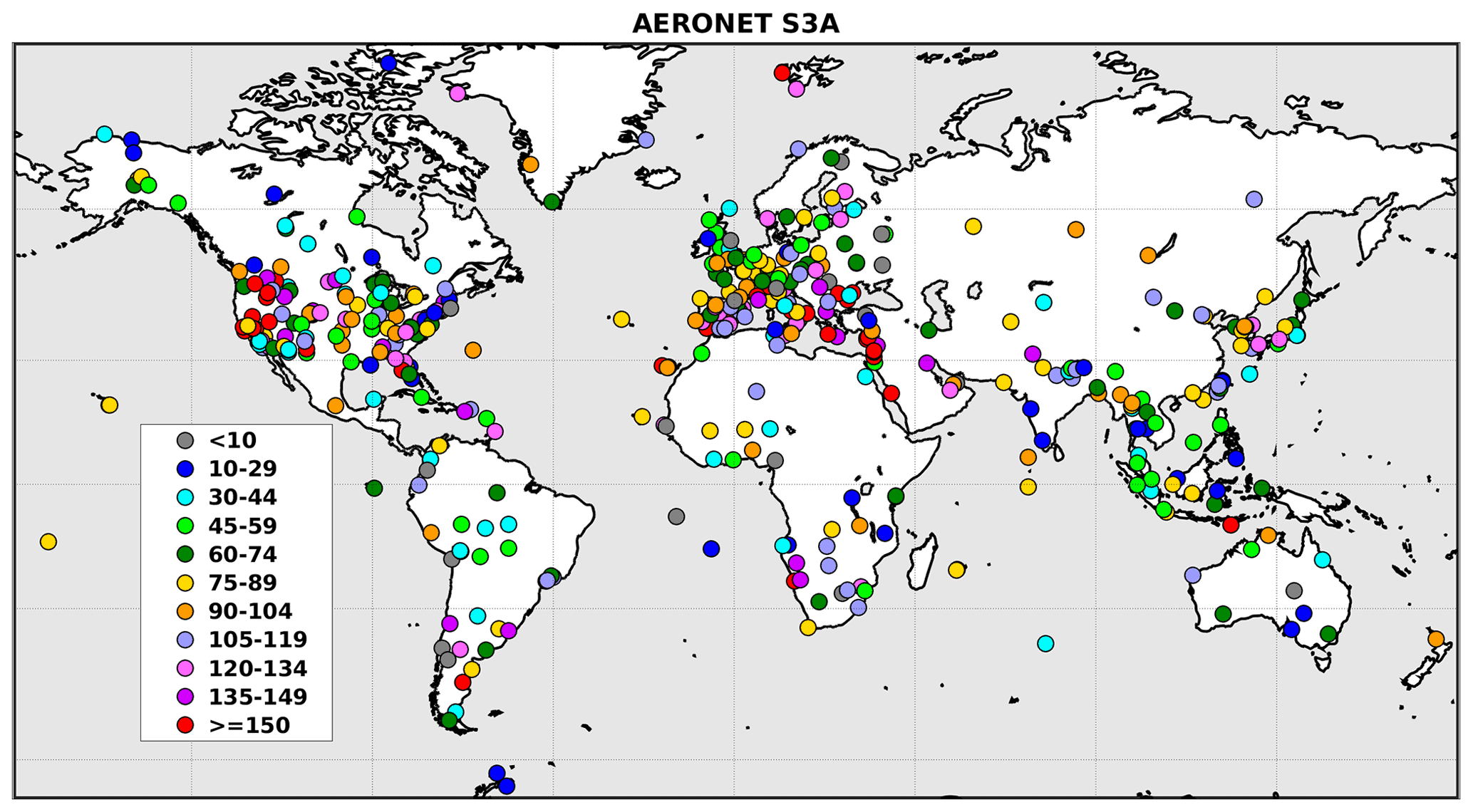
Figure 1 Location of the AERONET stations and number of matchups with S3A per station (see legend) for the period 14 January 2020 to 30 September 2021.

In the exercise it was found that the validation results for S3A and S3B are, in general, similar (difference between results for S3A and S3B is less than 10 % of S3A AOD). In this paper, validation results for S3A are shown in figures, while validation statistics for both S3A and S3B (shown as S3A/S3B) are summarised in tables and discussed.

6.1 AOD at 550 nm

AERONET does not provide AOD at 550 nm (this dataset will be referred to in the following as aAOD₅₅₀). AERONET AOD₄₄₀ (aAOD₄₄₀) and the AERONET Angström exponent for 440 and 870 nm (aAE_440–870) are used to calculate aAOD₅₅₀ following the AOD spectral dependence feature (a power-law relationship; Angström, 1929). However, aAOD₄₄₀ is not measured at all AERONET stations. For those stations, aAOD for another wavelength (400 nm or 500 nm) has been used to interpolate aAOD to 550 nm.

As shown in Fig. 1, AERONET stations are not evenly distributed globally. For the study period, more than 85 % of the matchups were from the NH. Thus, most global results were strongly influenced by the results obtained for the NH. In the case that validation results are similar for the globe and the NH, results for the globe are not visualised. In the case of a significant difference between the results for the globe and the NH, we show figures and discuss results for both. Validation statistics summarised in tables include results for the globe, NH, and SH.

6.1.1 Annual results

Scatter density plots for S3A SY_2 AOD₅₅₀ (syAOD₅₅₀, or syAOD) and corresponding AERONET AOD₅₅₀ (aAOD₅₅₀, or aAOD) for all matchups available for the NH and SH, including binned AOD offsets, are shown in Fig. 2. For most of the matchups (91 %), syAOD is small (< 0.4).

Figure 2 Scatter density plots for S3A syAOD₅₅₀ and corresponding aAOD₅₅₀ for all, dual, singleN, and singleO groups of matchups (panels top-down) available over the NH (left panels) and SH (right panels). The filled magenta circles are the averaged syAOD binned in 0.1 aAOD intervals, and the vertical lines on each circle represent the 1σ standard deviation of the fits.

Table 1 Validation statistics (number of points, N; percentage of matchups which fit into MODIS AOD error envelope, EE, defined as ±0.05 ± 0.2 × AOD; percentage of matchups which satisfy GCOS requirements of 0.03 or 10 % of AOD; correlation coefficient, R; root mean square, rms; standard deviation, σ; bias and slope defined with linear regression applied to all available matchups) for S3A and S3B syAOD₅₅₀ products for the globe, NH, and SH for the whole period for all matchups and for three groups of matchups, defined with the processor applied (dual, singleN, singleO).

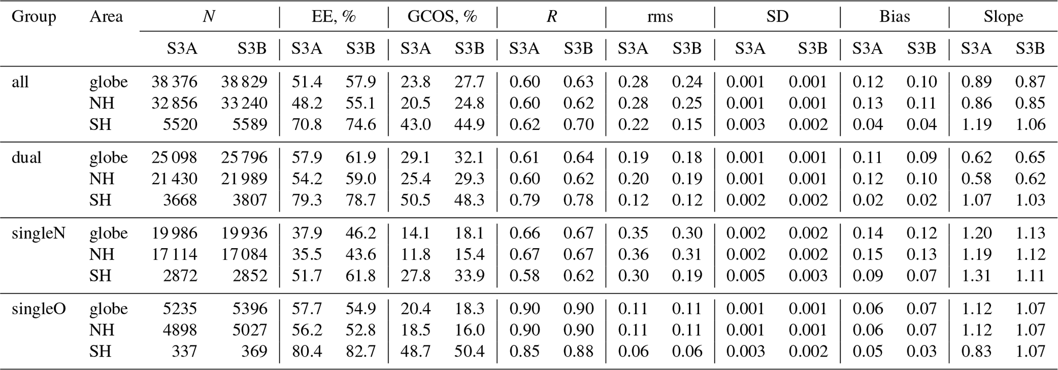
Validation statistics for S3A and S3B products are shown in Table 1. These include the number of points (N), the percentage of matchups which fit into the MODIS AOD error envelope (EE) defined as ±0.05 ± 0.2 × AOD (Remer et al., 2013), the percentage of matchups which satisfy Global Climate Observing System (GCOS) requirements of 0.03 or 10 % of AOD (GCOS, 2016), the Pearson correlation coefficient (R), root mean square (rms), standard deviation (SD), and bias and slope defined with linear regression (polynomial fit) applied to all available matchups.

A difference in the algorithm performance in the NH and SH is clear. For S3A, the fraction of matchups in the EE (70.8 %) and the fraction of matchups which satisfy GCOS requirements (43.0 %) are considerably higher in the SH (in the NH, 48.2 % and 20.5 %, respectively), but R (0.62) and rms (0.22) are only slightly better (in the NH, 0.6 and 0.28, respectively). For all matchups, validation statistics are better for S3B: in the SH, more matchups fit the EE (74.6 %) and GCOS (44.9 %); R (0.70) is higher and rms (0.15) is lower. In the NH, the difference between S3A and S3B is smaller.

In addition to the statistics shown in Table 1, we performed a respective analysis for limited AOD ranges. For aAOD < 1.5, syAOD validation statistics are slightly better than statistics for all aAOD ranges: bias is close to 0.1, and slope is close to 1 for both S3A and S3B AOD products in the NH. For aAOD > 1.5, bias is ca. 1.3 in the NH (where N is 127 and 125 for S3A and S3B, respectively). In the SH matchups available for the S3B product are located close to the 1 : 1 line; however, the number of matchups with aAOD > 1.5 is too small (N is $\mathrm{3}/\mathrm{2}$) to calculate validation statistics.

Group (dual, singleN, singleO) analysis reveals that most of the low-biased syAOD outliers were retrieved with the dual processor (Fig. 2), while most of the high-biased syAOD outliers were retrieved with the singleN processor. Total bias is smaller for the dual group globally and in both the NH and SH (Table 1). For aAOD < 1.5, syAOD bias is close to 0 for the dual group; for the singleN group bias is higher than for all matchups and increases with aAOD. Validation statistics are, in general, better in the SH (except for R for all the single groups). As for all matchups, validation statistics are slightly better for S3B.

Figure 3 For S3A, binned in 0.1 aAOD intervals, syAOD offsets (dAOD) for the globe (a), the NH (b), and SH (c) for all matchups, as well as the dual, singleN, and singleO groups of matchups (yellow rhombus, red, green, and blue dots, respectively; see legend).

Analysis of the binned (based on aAOD, bin size of 0.1) syAOD offsets to aAOD was carried out. For S3A (Fig. 3), the dual group shows better performance. In this group, the positive offset at low (< 0.2) AOD vanishes towards higher AOD and turns to negative at AOD > 0.4. About 91 % of matchups fit the AOD range of [0, 0.4]. In this AOD range, an offset is 0.03-0.05 higher in the NH compared with the SH. Offsets for the S3B in the same AOD range are lower (up to 0.03). Offsets for singleN and singleO groups are positive in the AOD range of [0, 1.2]. For high AOD, offsets are in general higher; however, less than 1.4 % of the matchups fit the range of aAOD > 1.

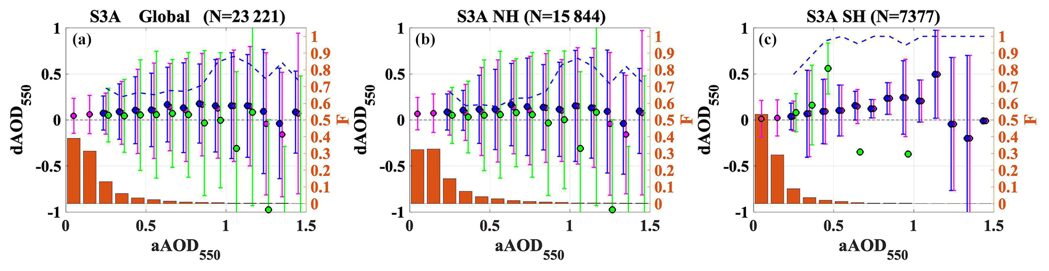
Figure 4 Global difference (a) as well as the NH (b) and SH (c) difference (dAOD₅₅₀) between syAOD and aAOD for aAOD binned in 0.2 intervals: median bias (circles) and bias standard deviation (error bars) for all and background (aAOD ≤ 0.2) AOD types (purple), as well as aerosol fine-dominated AOD (blue) and coarse-dominated AOD (green). The fraction (F) of points in each bin from the total number of matchups is represented by orange bars. The fraction of fine-dominated matchups in each bin is shown as the blue dashed line.

For the aAOD binned in 0.1 intervals, the global difference (dAOD) between syAOD and aAOD represented with the median bias and dAOD standard deviation is shown in Fig. 4 for all aerosol types including background (aAOD ≤ 0.2) AOD as well as fine-dominated and coarse-dominated AOD. Globally, background AOD (64 % from all matchups) is overestimated by 0.04–0.06. Overestimation of fine-dominated matchups increases from 0.07 to 0.15 in the AOD range of 0.2–1.2 (34 % of matchups). Overestimation for coarse-dominated matchups is about 0.05 for aAOD < 0.7; for aAOD of 0.7–0.9, an overestimation for coarse-dominated matchups is within the GCOS requirements of ± 0.03 dAOD. For aAOD > 1.2, dAOD varies in sign and amplitude; however, the number of matchups in this size range is low (< 1 %) and results are thus unstable. Fractions of the fine-dominated matchups per bin are 60 %–70 % for aAOD in the range of 0.2–0.9 and more than 70 % for aAOD > 0.9. Thus, binned offsets for all matchups closely follow offsets for fine-dominated matchups.

In the NH, the syAOD offset for the background matchups is ∼ 0.07; in the SH the offset is lower (< 0.02). Binned offsets for the fine-dominated and coarse-dominated matchups in the NH are similar to those for the globe. In the SH, offsets of syAOD are higher for aAOD > 0.4, where the number of the matchups per bin is low (< 50).

6.1.2 Monthly and seasonal results

Monthly (January, February, March, etc.), seasonal (DJF, MAM, JJA, SON), and annual (year) variations of the validation results for S3A and S3B syAOD₅₅₀ for the globe, NH, and SH are shown in Fig. 5.

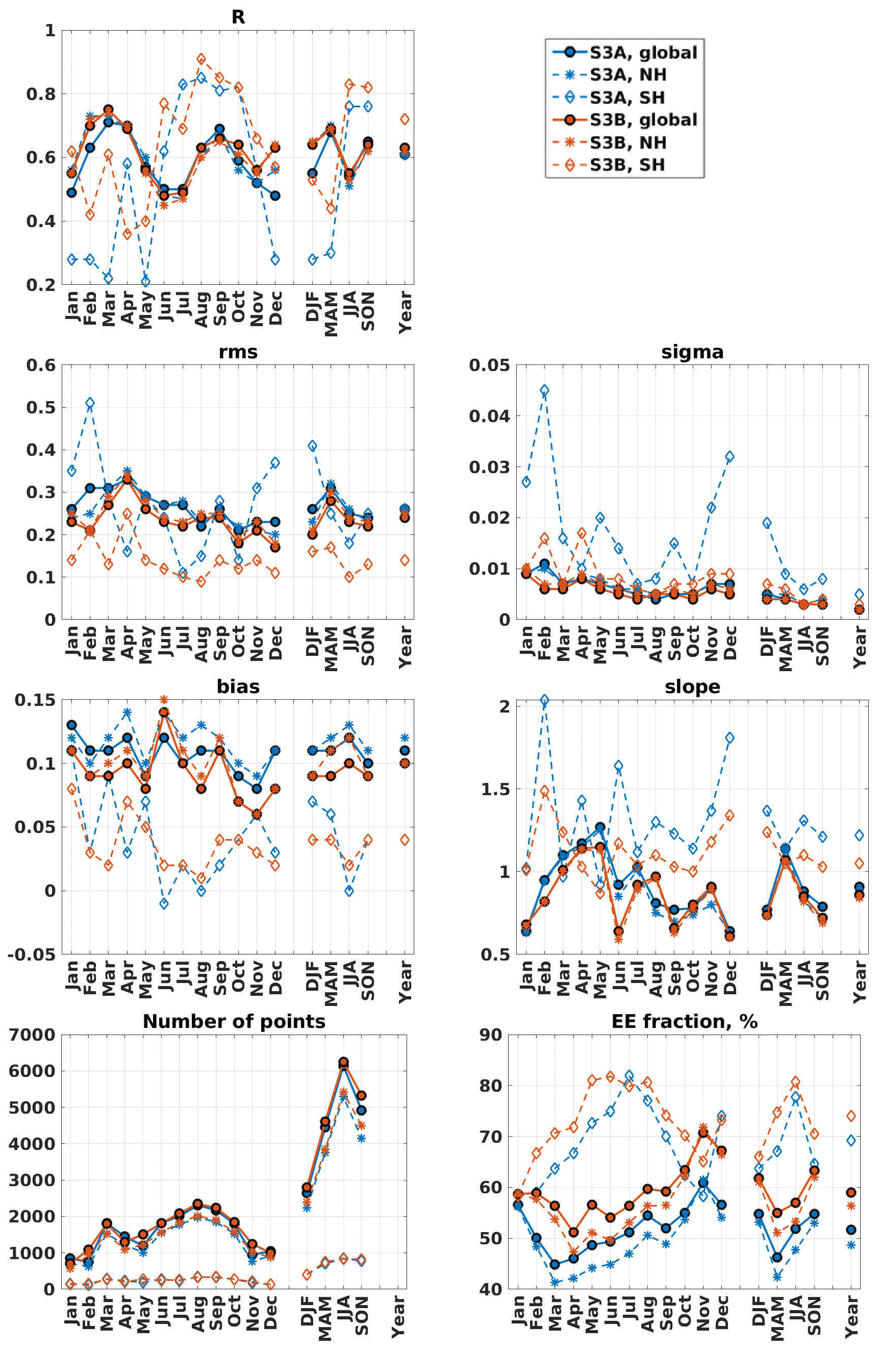
Figure 5 Validation statistics for syAOD₅₅₀ aggregated monthly (January, February, and so on), seasonally (DJF, MAM, JJA, SON), and yearly (Year) shown as time series for S3A and S3B for the globe, NH, and SH.

The correlation coefficient R is of sinusoidal shape for monthly statistics with two maxima for both S3A and S3B in the NH. In the SH, the correlation coefficient varies strongly along the year. A clear peak (0.8–0.9) for both S3A and S3B is observed in June–October. The rms in the NH is within 0.25–0.32 for both S3A and S3B, with a minimum in October–January and a maximum in March–May. In the SH, rms for S3B is 0.15–0.2 in December–May and 0.09–0.14 in the other months.

Bias varies from 0.06 to 0.14 in monthly statistics in the NH. In the SH, bias is lower; it varies from 0.01 to 0.08 in monthly statistics. For S3B, bias is 0.01–0.35 lower than for S3A in all months, except April.

The fraction of matchups in the EE reflects the difference between the NH and SH and between S3A and S3B well. EE is, in general, higher for S3B with the offset up to 15 % in the NH.

As a short summary, syAOD₅₅₀ validation results are slightly better for S3B; the retrieval algorithm produces better results in the SH. Obtained validation results confirm that backscatter contribution to the radiance measured at the top of the atmosphere is less critical in the SH.

6.1.3 Regional performance

There are noticeable regional differences in the performance of the retrieval algorithm, which depend on e.g. AOD load and AOD types (composition and optical properties), as well as on the properties of underlying surfaces. Retrieval quality (accuracy, precision, and coverage) varies considerably as a function of these conditions, as well as whether a retrieval is performed over land or over ocean.

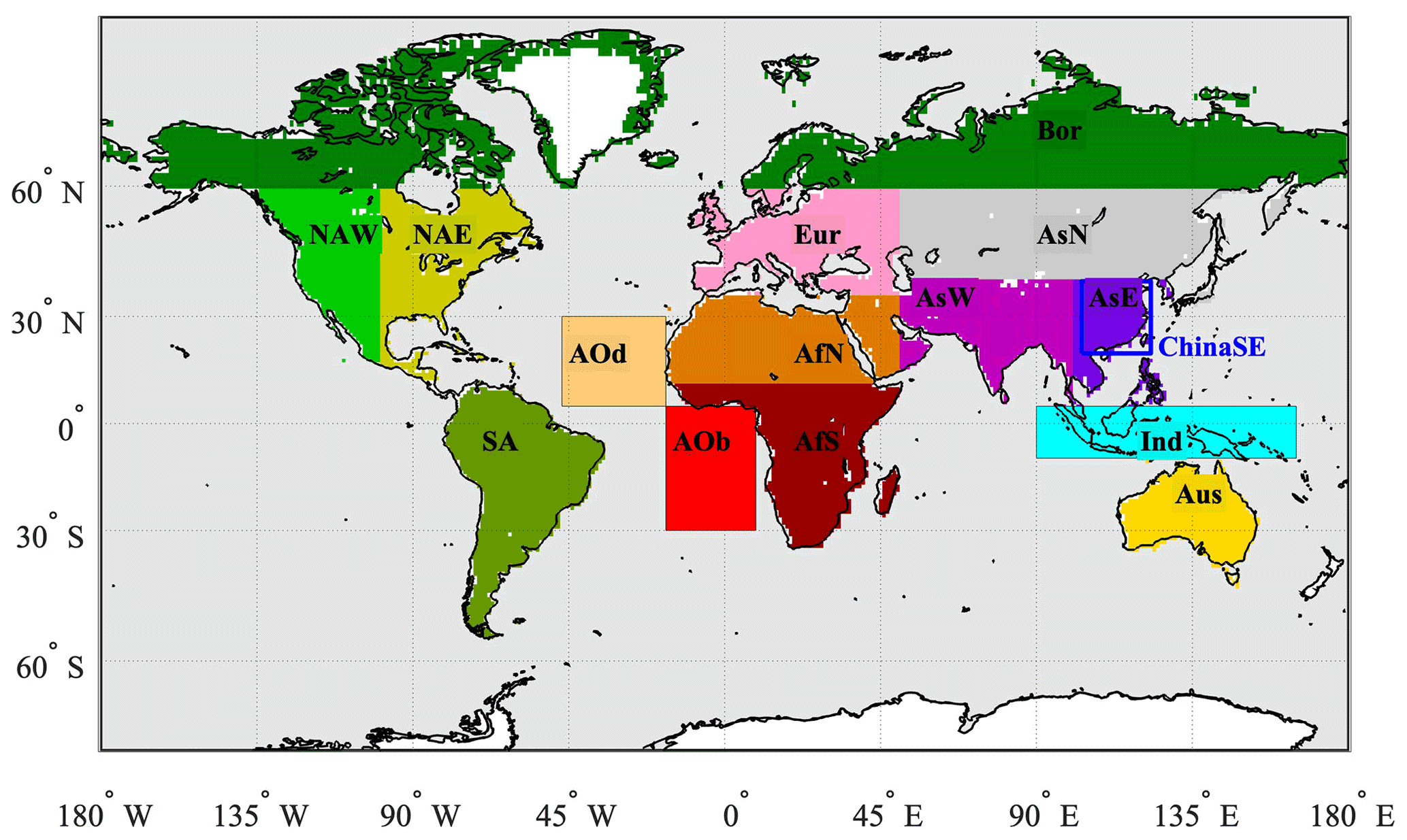
Figure 6 Land and ocean regions defined for this study (as in Sogacheva et al., 2020): Europe (Eur), boreal (Bor), northern Asia (AsN), eastern Asia (AsE), western Asia (AsW), Australia (Aus), northern Africa (AfN), southern Africa (AfS), South America (SA), eastern North America (NAE), western North America (NAW), Indonesia (Ind), Atlantic Ocean dust outbreak (AOd), and Atlantic Ocean biomass burning outbreak (AOb). In addition, southeastern China (ChinaSE), which is part of the AsE region marked with a blue frame, is considered separately. Land, ocean, and global AOD was also considered.

Following Sogacheva et al. (2020), we intercompare validation results over 15 regions (as defined in Fig. 6) that seem likely to represent a sufficient variety of aerosol and surface conditions. These and include 11 land regions, two ocean regions, and one heavily mixed region. The land regions represent Europe (denoted by Eur), boreal (Bor), northern, eastern, and western Asia (AsN, AsE, and AsW, respectively), Australia (Aus), northern and southern Africa (AfN and AfS), South America (SA), and eastern and western North America (NAE and NAW). Southeastern China (ChinaSE), which is part of the AsE, is considered separately. The Atlantic Ocean is represented as two ocean regions, one characterised by Saharan dust outflow over the central Atlantic (AOd) and a second that includes burning outflow over the southern Atlantic (AOb). The mixed region over Indonesia (Ind) includes both land and ocean. For exact locations, see Table S2 in the Supplement.

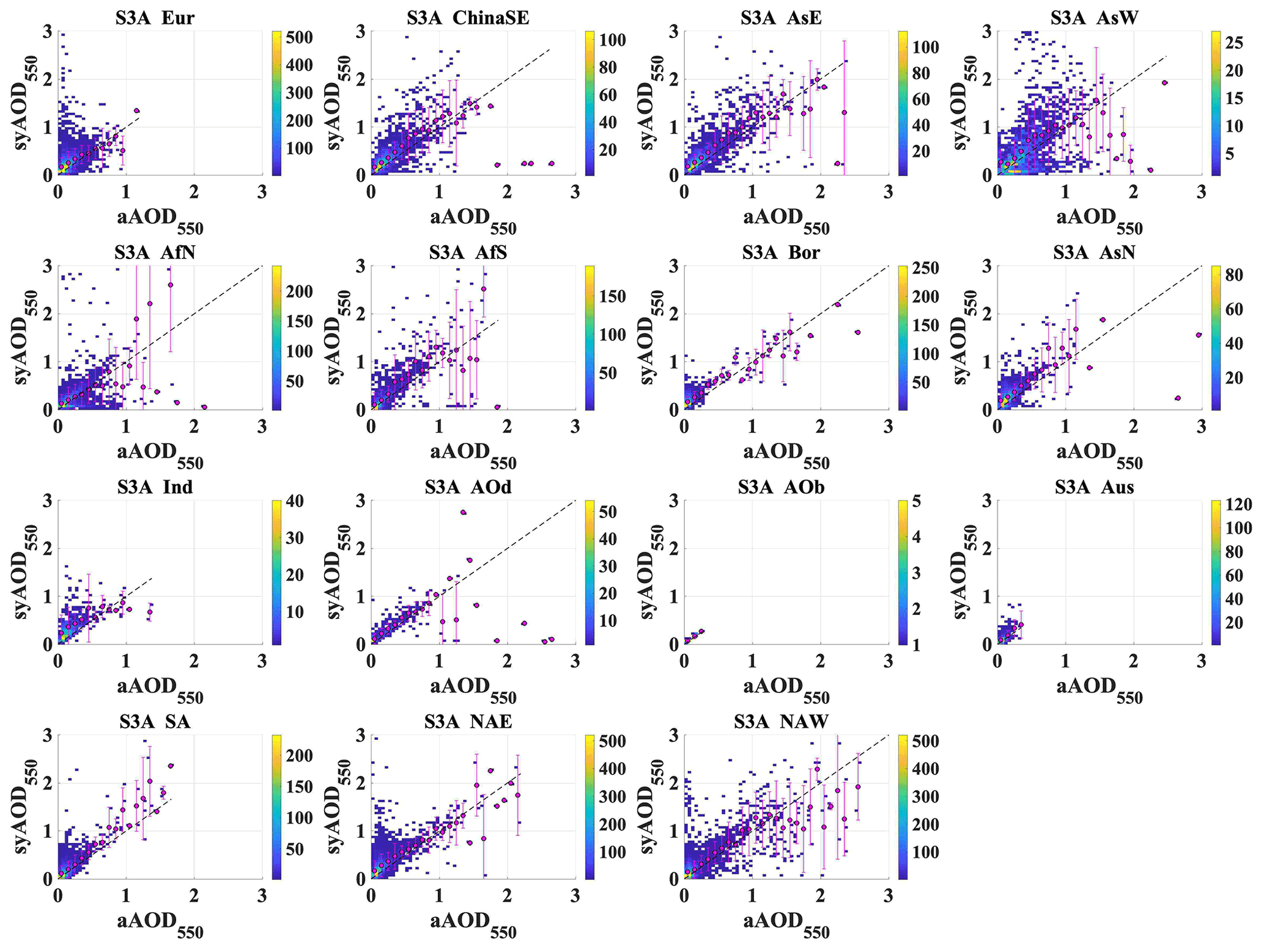
Figure 7 For S3A, syAOD and aAOD scatter density plots for selected regions (as defined in Fig. 6).

High diversity in the validation results was observed between the selected regions (Fig. 7; Table S2 in the Supplement). The highest correlation (0.94) was found in AOb region (the number of matchups is low in this region at 22). For ChinaSE, AsN, AsE, AOd, Aus, and NAE, the correlation coefficient R was in the range 0.6–0.8, which was higher than that for the globe. For Eur and Ind, R < 0.4. For the above-mentioned regions, bias between binned syAOD and aAOD does not change much. Bias is positive in Asia, Bor, and SA regions for aAOD ≲ 1.2; bias calculated with linear regression was higher for those regions. The number of syAOD outliers, defined as |syAOD − ​​​​​​​aAOD| > 0.5, varied among the regions. In Eur, positive syAOD outliers were observed for aAOD < 0.3. For Asian and Bor regions, syAOD outliers were observed mostly for aAOD in the range of [0.2, 1.2]. More negative syAOD outliers were observed in the NAW region.

Among the land regions, the fraction of the pixels in EE was highest in Aus (81.6 %) and lowest in Bor and SA (< 30 %); for other land regions the fraction of the pixels in EE was in the 30 %–60 % interval. Over ocean, in AOb and AOd areas, the fraction of the pixels in EE was high (67.8 % and 95.5 %, respectively).

The fraction of syAOD pixels which satisfy GCOS requirements was low (< 31 %) for all regions, except for Aus (54.5 %) and AOb (68.2 %), where matchups cover low-AOD (< 0.3) conditions only.

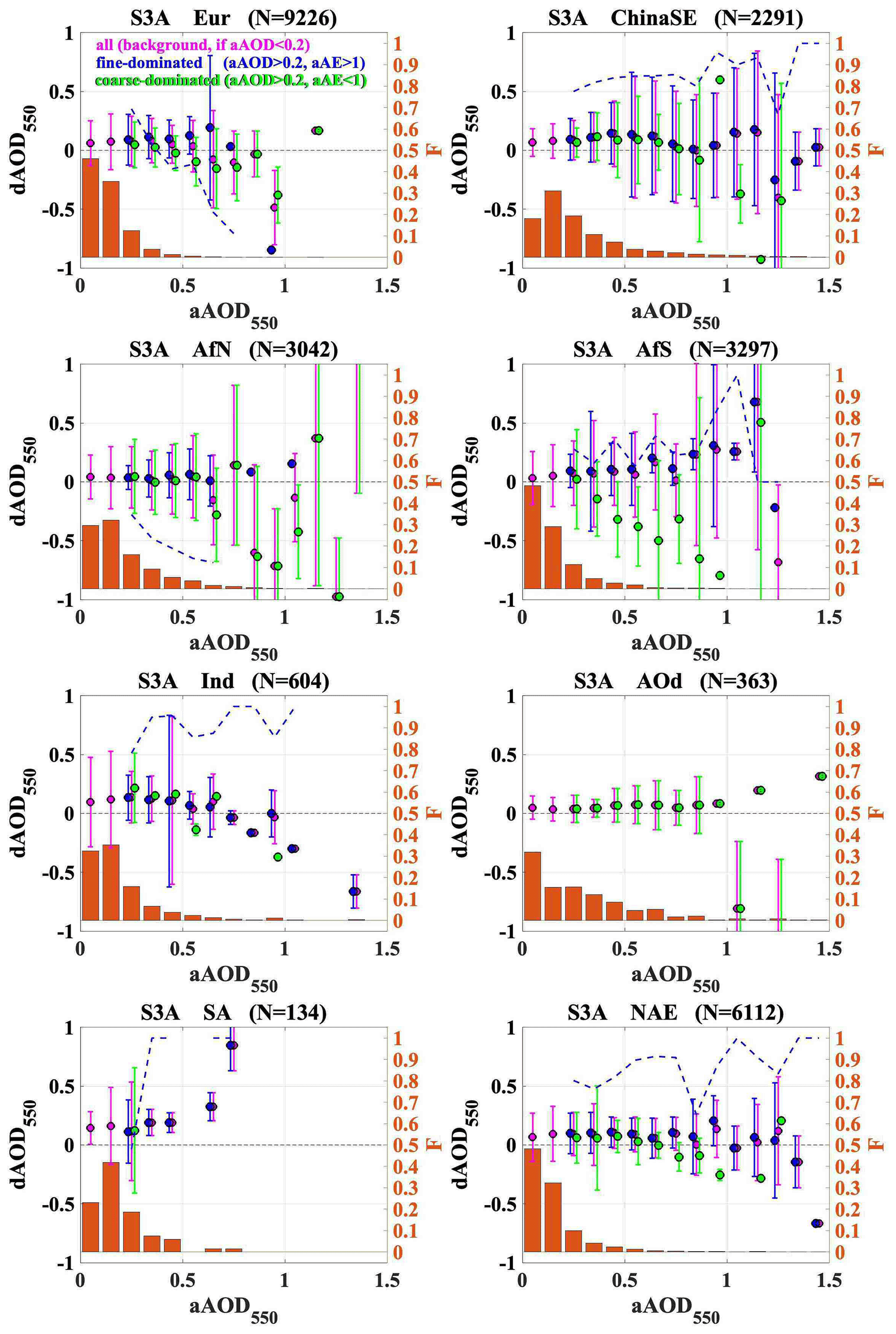
Figure 8 Regional (for Eur, ChinaSE, AfN, AfS, Ind, AOd, SA, NAE) difference (dAOD₅₅₀) between syAOD and aAOD for aAOD binned in 0.1 intervals: median bias (circles) and bias standard deviation (error bars) for all and background (aAOD ≤ 0.2) AOD types (purple), as well as aerosol fine-dominated AOD (blue) and coarse-dominated AOD (green). The fraction (F) of points in each bin from the total number of matchups is represented by orange bars. The fraction of fine-dominated matchups in each bin is shown as a blue dashed line. Results for other regions are in the Supplement (Fig. S7).

Regional differences between syAOD and aAOD for all aerosol types including background (aAOD ≤ 0.2) AOD as well as fine-dominated and coarse-dominated AOD for selected aAOD bins are shown in Fig. 8. For most of the regions, a general tendency towards positive SY_2 AOD offsets is observed under the background conditions. Offsets are higher (up to 0.15) in Ind and SA and lower (< 0.04) in AfN, AfS, and AOd. The behaviour of the fine-dominated offset is similar for most of the regions (ChinaSE, AfN, AfS, Ind) with a gradual increase in the aAOD range of ca. 0.7–1.1. The coarse-dominated offset over Eur is underestimated by up to 0.18 for aAOD of 0.6–0.8. Over China, the coarse-dominated offset is slightly overestimated at aAOD < 0.7 and underestimated at aAOD > 1. Over bright surface with a contribution of dust aerosols (AfN), all groups show good agreement with aAOD for aAOD < 0.7. For aAOD > 0.7, syAOD for coarse-contaminated matchups is considerably underestimated. Similar offsets are observed in the NAE region, where 70 %–90 % of matchups are characterised by fine-dominated aerosols. In the possible biomass burning region (AfS), an underestimation of syAOD for coarse-dominated matchups gradually increases for aAOD > 0.3, reaching −0.9 at aAOD close to 1. Over Ind, dAOD is positive for aAOD < 0.5. Over ocean, with possible contamination of Saharan dust (AOd), offsets are constantly positive (up to 0.1) for all groups at aAOD < 1.

6.1.4 Analysis of syAOD relative offsets

The syAOD offset analysis was performed for matchups which did not satisfy the GCOS requirements of |syAOD − aAOD| < 0.03 or |syAOD − aAOD| < 0.1 × aAOD (GCOS, 2016).

The syAOD relative offset, or dAOD,rel, was defined as in Eq. (1).

$$\begin{array}{}\text{(1)}& \text{dAODrel}={\displaystyle \frac{\text{syAOD}-\text{aAOD}}{\text{aAOD}}}\end{array}$$

Latitude dependence of the syAOD relative offset

In Fig. 9 we show a density scatter plot for the latitude dependence of the relative offset of the syAOD for all, dual, singleN, and singleO groups of pixels for S3A. Colour indicates the fraction of the points with corresponding dAOD,rel from the total number of points within the 10^∘ latitude bin. As an example, for the latitude 20–30^∘ S, dAOD,rel was between −0.5 and −1 for ∼ 38 % of matchups. The magenta line shows the number of matchups in the x-axis bin.

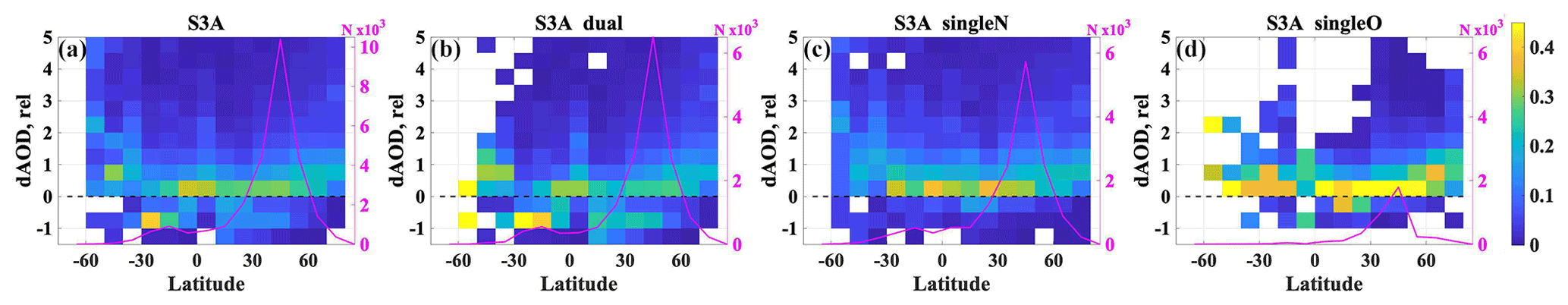
Figure 9 For S3A, density scatter plot for the latitude (in degrees) dependence of the syAOD relative offset for all (a), dual (b), and singleN (c) groups of pixels. Colour indicates the fraction of the points with a corresponding dAOD,rel interval from the total number of points within the latitude bin. The magenta line shows the total number of matchups in the corresponding latitude bin.

In the NH, dAODrel was mostly positive (syAOD was higher than aAOD). In the SH, dAOD,rel is mostly positive at 30–60^∘ S and mostly negative at 10–30^∘ S, except for the singleN group, for which dAOD,rel is mostly positive. In both NH and SH, dAOD,rel increases towards the poles. This increase is more pronounced for the singleO group of pixels but also visible in the dual group.

Dependence of syAOD relative offset on surface reflectance

The directional surface reflectance (SR) retrieved with the SYNERGY algorithm is provided in the SY_2_AOD product.

Figure 10 For S3A syAOD matchups with AERONET which do not satisfy GCOS requirements, scatter density plot for the dependence of the syAOD relative offset of retrieved surface reflectance for all (a), dual (b), and singleN (c) groups of pixels. Colour indicates the fraction of the points with a corresponding dAOD,rel interval from the total number of points within the surface reflectance bin. The magenta line shows the total number of matchups in the corresponding surface reflectance bin.

In Fig. 10 we show a density scatter plot for the dependence of the relative offset of the AOD on the retrieved SR for the dual, singleN, and singleO groups of matchups. Colour indicates the fraction of the points with corresponding dAOD,rel from the total number of points within the surface reflectance bin.

For all matchups (not shown here), as well as for the dual group (globally, as well as over the NH and SH), footprints for the dAODrel dependence on the SR are similar. For SR < 0.05 and SR > 0.35, dAOD,rel indicates that syAOD is mostly overestimated. In specified ranges, dAOD,rel increases towards outer edges. For the SR in the range of 0.05–0.35, syAOD is mostly underestimated. Underestimation is more pronounced when syAOD is retrieved with the dual processor. For the singleO group, syAOD is mostly overestimated in all SR ranges.

Dependence of the AOD relative offset on solar and satellite geometry

In Fig. 11 we show the dependence of the syAOD relative offsets on the OLCI geometry (relative azimuth (Raz), satellite zenith angle (SatZA), and sun (or solar) zenith angle (SunZA) provided in the SY_2_AOD product (North and Heckel, 2019) for the NH and SH. Colour indicates the fraction of the points with a corresponding dAOD,rel interval in the Raz, SatZA, or SunZA bins.

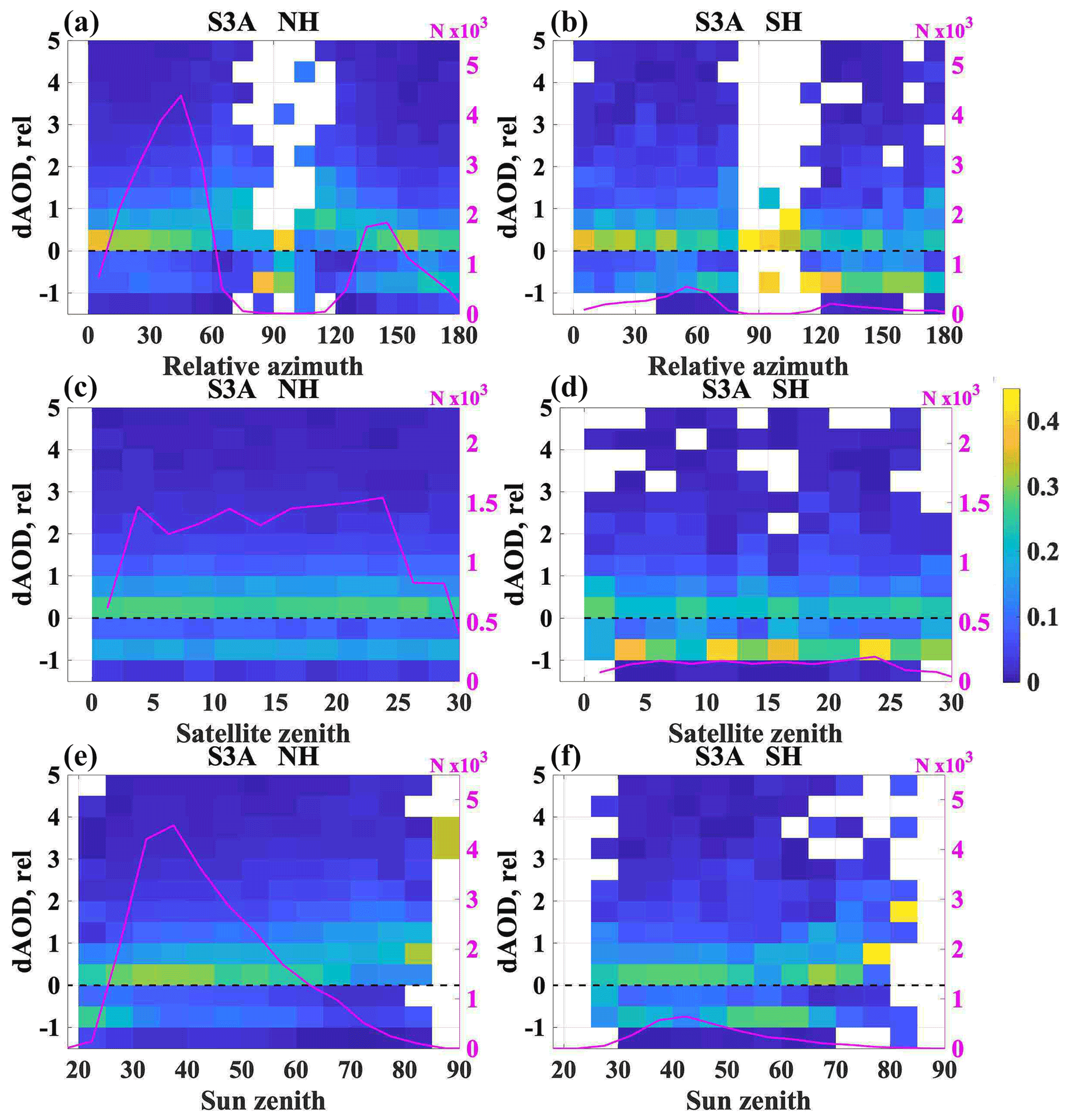
Figure 11 For S3A syAOD matchups with AERONET which do not satisfy GCOS requirements, the dependence of the AOD relative offsets on relative azimuth (a, b), satellite zenith angle (c, d), and sun zenith angle (e, f) for the NH (a, c, e) and SH (b, d, f) for all pixels. Colour indicates the fraction of the points with corresponding dAOD,rel from the total number of points within the x-axis bin. The magenta line shows the total number of matchups in the corresponding x-axis bin.

In the NH, positive dAOD,rel increases with Raz increasing from 50 to 80^∘ and decreases with Raz increasing from 100 to 140^∘. In the SH, we see a similar dependence of dAOD,rel for Raz at 50–80^∘. For Raz > 90^∘, positive dAOD,rel increases with a Raz increase from 150 to 180^∘; a negative dAOD,rel of [−1, −0.5] is observed more often than positive [0, 0.5] dAOD,rel.

No significant dependence of dAOD,rel on the SatZA was observed. However, a greater number of negative dAOD,rel values is clearly seen in the SH.

In the NH, dAODrel is slightly positive (0–0.5) in all ranges of SunZA, except for the most extreme values. For SunZA > 80^∘, the percentage of higher positive dAOD,rel (0.5–1) increases, while for SunZA < 30^∘ the percentage of higher negative dAOD,rel rises. In the SH, a similar dependence was observed, except for SunZA in the range of 50–65^∘, where dAOD,rel is mainly negative.

6.1.5 Linear regression considering provided syAOD uncertainties

Linear fitting for combinations of syAOD₅₅₀ and aAOD₅₅₀ collocations has been performed with a consideration of the syAOD₅₅₀ and aAOD₅₅₀ uncertainties (https://se.mathworks.com/help/stats/linearmodel.predict.html, last access: 8 March 2022). For syAOD₅₅₀, pixel-level uncertainties are provided in the SY_2_AOD product. For aAOD₅₅₀, uncertainty of 0.01 has been considered (Eck et al., 1999). For both S3A and S3B, for all groups of matchups, bias and slope for the linear regression fits applied to the whole AOD range were improved when the syAOD and aAOD uncertainties were considered. Bias was lowered by roughly 50 %. Slope was improved by 10 %–15 %. Improvements were smaller for the singleO group of matchups (retrievals over ocean), for which the syAOD uncertainties are smallest (Sect. 6.2).

For more details, see Fig. S8 and Table S3, which are both in the Supplement.

6.1.6 AOD at wavelengths other than 550 nm

Scatter plots for SY_2 AOD₄₄₀, AOD₆₇₀, AOD₈₆₅, and AOD₁₆₀₀ are shown in Fig. 12. Clear tendencies in validation statistics were observed when comparing validation results from shorter (440 nm) to longer (1600 nm) wavelengths. Though the correlation coefficient decreases (0.65, 0.55, 0.50, and 0.40 for 440, 670, 865, and 1600 nm, respectively), the offset (0.15, 0.1, 0.07, 0.05) and rms (0.33, 0.23, 0.18, 0.16) also decrease. Note that AOD decreases significantly (except for dust aerosols) as wavelength increases.

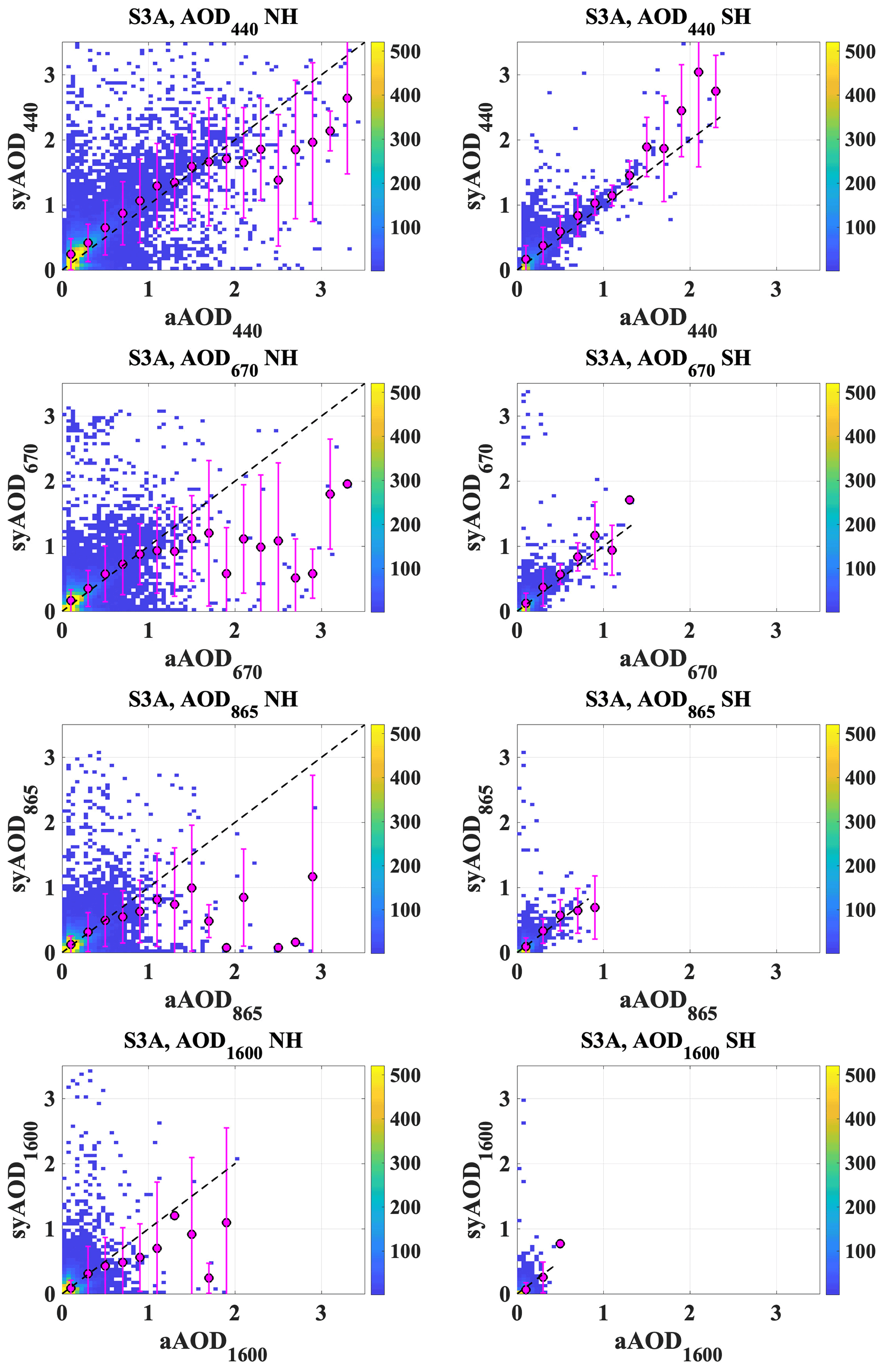
Figure 12 Scatter plots for SY_2 AOD₄₄₀, AOD₆₇₀, AOD₈₇₀, and AOD₁₆₀₀ (panels top down) for the NH and SH (left and right panels, respectively).

Validation statistics for all wavelengths are slightly worse for the NH than global validation statistics (Table S4, Supplement); validation statistics for the SH are considerably better than for the NH (except for R for 1600 nm wavelength).

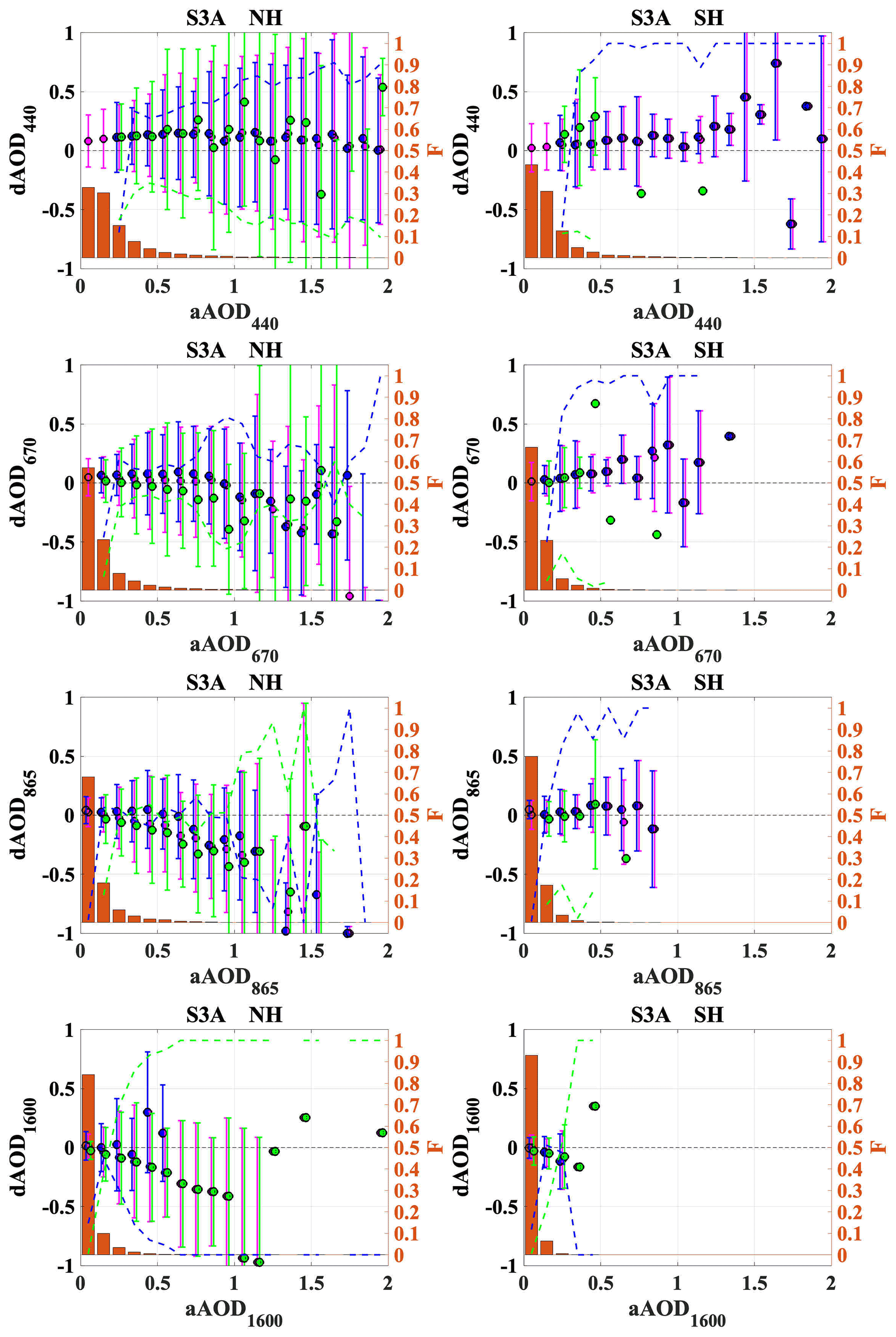
Figure 13 For​​​​​​​ the NH (left) and SH (right) for different wavelengths (top down: 440, 670, 865, 1600 nm), the difference (dAOD₅₅₀) between syAOD and aAOD for selected aAOD bins: median bias (circles) and bias standard deviation (error bars) for all (incl. background, aAOD₅₅₀ ≤ 0.2) AOD types (purple), as well as aerosol fine-dominated AOD (blue) and coarse-dominated (green) AOD. The fraction (F) of fine-dominated matchups from the total number of matchups in each bin is represented by orange bars. The fractions of fine- and coarse-dominated matchups in each bin are shown as blue and green dashed lines, respectively.

The syAOD₄₄₀ is overestimated for all aerosol types (Fig. 13). The syAOD₆₇₀ for fine-dominated matchups is in good agreement with aAOD₆₇₀ for aAOD₆₇₀ < 1. A similar tendency, though for narrower aAOD ranges (aAOD₈₇₀ < 0.5 and aAOD₁₆₀₀ < 0.3), is observed for syAOD₈₆₅ and syAOD₁₆₀₀. For all wavelengths, coarse-dominated syAOD is retrieved accurately for aAOD below ca. 0.4; above 0.4 syAOD is underestimated, and the offset between syAOD and aAOD increases with increasing aAOD.

6.2 AOD uncertainties

The concept for validation of the AOD uncertainties applied in the current study follows the validation strategy suggested by Sayer et al. (2013, 2020) with consideration of the validation practice further developed in the ESA Aerosol_cci+ project (Product Validation and Intercomparison Report, https://climate.esa.int/media/documents/Aerosol_cci_PVIR_v1.2_final.pdf, last access: 25 February 2022).

Definitions for uncertainties in the current evaluation of uncertainties are as follows.

• Prognostic (per-retrieval) uncertainties (PUs) for the AOD product are provided at 440, 550, 670, 865, 1600, and 2250 nm wavelengths.

• Expected discrepancy (ED) is an uncertainty variable which accounts for the PU and the accuracy of the ground-based (AERONET) data (AU), as defined by Sayer et al. (2020) in Eq. (2):

  $$\begin{array}{}\text{(2)}& \mathrm{ED}=\sqrt{{\mathrm{PU}}^{\mathrm{2}}+{\mathrm{AU}}^{\mathrm{2}}}\end{array}$$

  According to Giles et al. (2019), AU = 0.01.

• AOD error (AODerror) is the difference between a satellite product AOD (syAOD) and AERONET AOD (aAOD); AOD absolute error (absAODerror) is an absolute value for AOD error.

Mean bias correction has been performed for the error distributions in some of the subsequent analysis, since the concept of standard uncertainties requires bias-free error distributions which can be interpreted as an absence of remaining systematic and quantifiable biases (https://climate.esa.int/media/documents/Aerosol_cci_PVIR_v1.2_final.pdf, last access: 25 February 2022).

If wavelength is not specifically mentioned, all variables in Sect. 6.2 refer to the wavelength of 550 nm.

Analysis of the distribution of the uncertainties has been performed for the whole S3A and S3B SY_2_AOD product, as well as for groups of pixels retrieved with different retrieval approaches (dual, singleN, singleO). Results for S3A and S3B are similar; only results for S3A are shown and discussed.

6.2.1 χ2 test for evaluation of the prognostic uncertainties

The goodness of the predicted uncertainties was estimated with the χ2 test, as in Eq. (3)

$$\begin{array}{}\text{(3)}& \mathit{\chi }\mathrm{2}={\displaystyle \frac{\mathrm{1}}{N-\mathrm{1}}}\sum _{i=\mathrm{1}}^N{\stackrel{\mathrm{‾}}{\mathit{\delta }}}_i,\end{array}$$

with individual weighted deviation ${\stackrel{\mathrm{‾}}{\mathit{\delta }}}_i$ described in Eq. (4).

$$\begin{array}{}\text{(4)}& {\stackrel{\mathrm{‾}}{\mathit{\delta }}}_i={\displaystyle \frac{{\left({\text{syAOD}}_i-{\text{aAOD}}_i-\text{mean}(\text{syAOD}-\text{aAOD})\right)}^{\mathrm{2}}}{{\text{PU}}_i^{\mathrm{2}}+{\text{AU}}^{\mathrm{2}}}}\end{array}$$

If χ2 ∼ 1, prognostic uncertainties describe the AOD error well. If χ2 ≫ 1, PUs are strongly underestimated; if χ2 ≪ 1, PUs are strongly overestimated. χ2 was calculated for the whole dataset and for different AOD bins to reveal if the goodness of the PU uncertainties is AOD-dependent.

For the whole dataset, χ2 = 3.1, which means that PUs are slightly underestimated. For the binned AOD, χ2 varies strongly (Fig. 14). For aAOD < 0.4, which is ca. 90 % of all values, χ2 fits into the interval [1.8, 3.2]. Thus, for most of the matchups, PU is only slightly underestimated. For AOD > 0.4 PU underestimation is more pronounced.

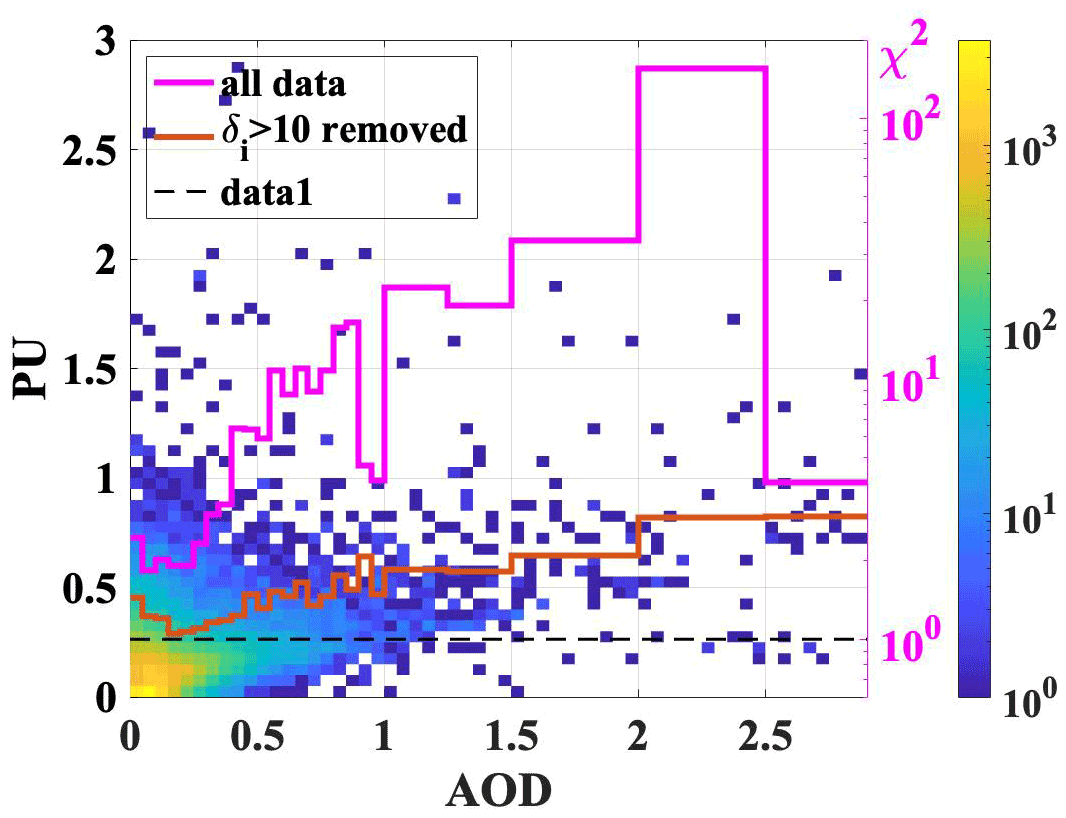
Figure 14 χ2 for binned aAOD for all available matchups (magenta line) and after the outliers of the individual weighted deviations (${\stackrel{\mathrm{‾}}{\mathit{\delta }}}_i$ > 10) are removed (red line). Density scatter plot for PU and syAOD.

No significant dependence of ${\stackrel{\mathrm{‾}}{\mathit{\delta }}}_i$ on AOD error or surface reflectance provided in the SY_2_AOD product has been revealed (Fig. S9, Supplement).

Though the number of matchups in the whole dataset is high (which provides confidence in χ2 test results), it was noticed that high ${\stackrel{\mathrm{‾}}{\mathit{\delta }}}_i$ (up to 155) exists, which may bias the evaluation of the PU with χ2. To remove possible contribution of the outliers to the χ2 test results, cases with ${\stackrel{\mathrm{‾}}{\mathit{\delta }}}_i>\mathrm{10}$ (which make up less than 5 % of the total number of matchups) were removed from the analysis.

For the dataset with the removed outliers, χ2 = 1.2, which means that PUs describe the AOD error well.

The influence of ${\stackrel{\mathrm{‾}}{\mathit{\delta }}}_i$ outliers is more pronounced for AOD bins, in which number of matchups per bin is lower and thus the contribution of the outliers to the results is more expected. If ${\stackrel{\mathrm{‾}}{\mathit{\delta }}}_i$ outliers are removed from the binned analysis, χ2 fits the range [1, 1.45] for AOD < 0.4 (Fig. 14).

6.2.2 Evaluation of prognostic uncertainties with absolute AOD error

To qualitatively illustrate the accuracy of prognostic uncertainties, we show in Fig. 15 the comparison between the PU, AOD error distribution, and theoretical Gaussian distribution (with a mean of 0 and standard deviation of the syAODerror). PU distribution shows a double peak (the first peak is at ca. 0.02–0.04 for all groups; the second peak is in a range of 0.12–0.18 for different groups). For singleN, two peaks are located close to each other. Mean PU for the dual group is higher; SD is higher for the singleN group. AOD error distributions are Gauss-like with some asymmetry in the positive AOD error direction.

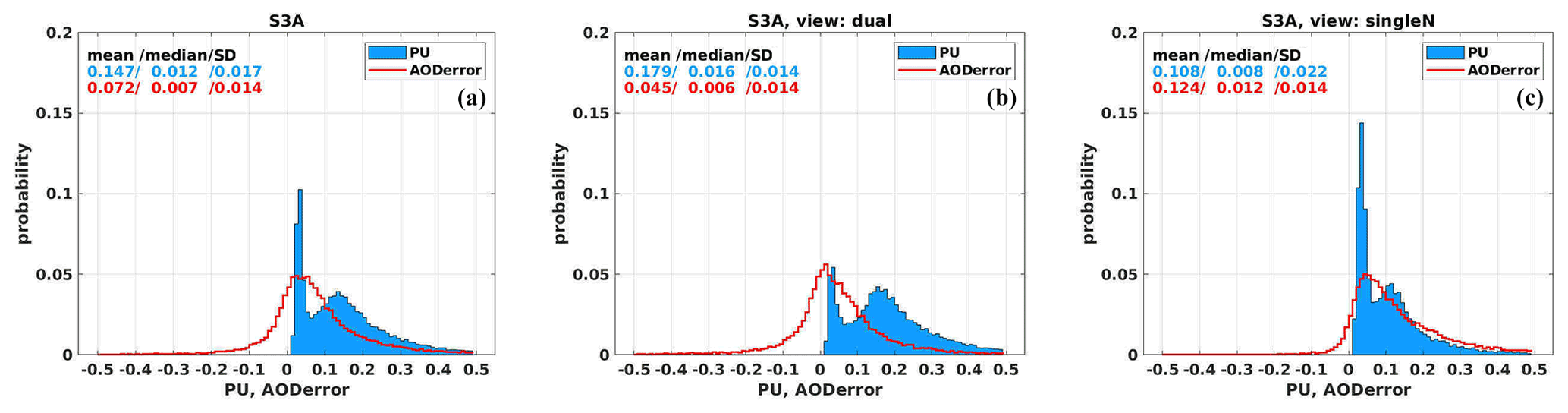
Figure 15 Comparison between PU, AOD error distribution, and theoretical Gaussian distribution for the whole product (a) as well as dual (b) and singleN (c) groups of matchups.

6.2.3 Evaluation of expected discrepancy and absolute AOD error

ED is calculated for each pixel by combining PU and AERONET uncertainties, as in Eq. (2).

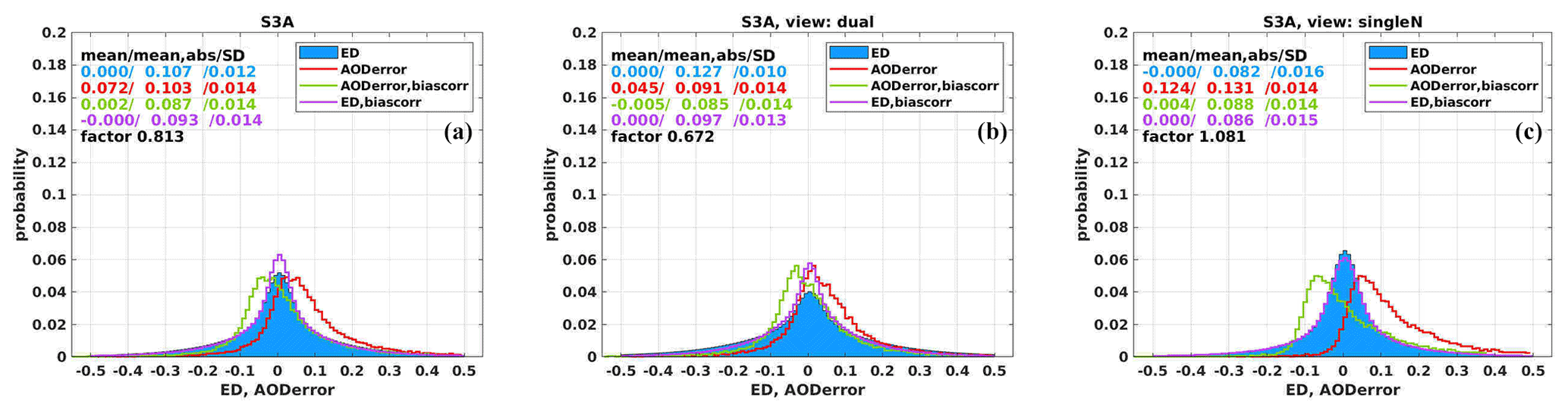
Figure 16 Histograms of the ED (blue filled bars), AOD errors (red; with bias correction: green), and ED calculated from uncertainties (purple; scaled to best fit the mean-bias-corrected error distribution) for all matchups (a) as well as dual (b) and singleN (c) groups of matchups. The statistics of mean, mean,abs, and SD are means over “real” values, means over “absolute” values, and standard deviation, respectively, for histograms of the corresponding colour.

For a quantitative validation, we follow (with some modifications) a new approach developed by ESA Aerosol CCI (https://climate.esa.int/media/documents/Aerosol_cci_PVIR_v1.2_final.pdf, last access: 25 February 2022). A synthetic cumulative distribution of ED is calculated assuming a Gaussian error distribution (normalised to a total integral of 1) with standard deviation of ED. In the next step, this synthetic error frequency distribution is compared with the AOD error. We calculate and subtract the mean bias from the AOD error distribution to make it more symmetric for direct comparison to the synthetic distribution (which by definition is always symmetric). Bias correction results for S3A all, dual, and singleN (0.07, 0.04, and 0.12, respectively) are shown in Fig. 16.

Finally, we calculate an average correction factor for the synthetic distribution (and thus the prognostic uncertainties) in relation to the mean-bias-corrected error distributions as the ratio of the absolute means of both distributions. Correction factors are different for all matchups and for the dual and singleN groups. A small correction is needed for all and singleN (0.80 and 1.1, respectively). For the dual group, the correction is stronger (0.67); ED should be lowered.

However, the correction method applied here does not equally improve ED in all ranges. The correction factor is biased by the number of pixels with small (< 0.2) absAODerror. Thus, for those cases the correction works well; overestimated ED is lowered by 0.8 and 0.65 for the all and dual groups. For absAODerror ≳ ​​​​​0.3, where ED is underestimated, correction degrades ED and increases disagreement between ED and AOD error. A possible solution can be to perform correction separately for different absAODerror ranges, but setting specific relations for different groups between ED and absAODerror makes the analysis very complicated.

6.2.4 Potential of the expected discrepancy

Sayer et al. (2020) suggested the analysis of the potential of the PU to discriminate between (“good” and “bad”) pixels with likely small or large errors. Instead of PU, we perform analysis of the ED, which, besides PU, includes uncertainties of the ground-based measurements.

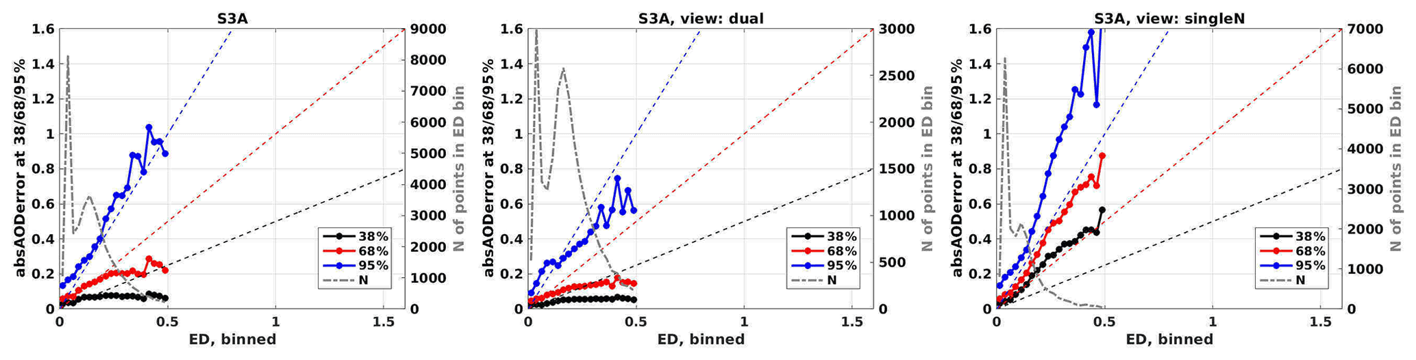
Figure 17 Percentile plots of absolute AOD errors at 38 % (black), 68 % (red), and 95 % (blue) as a function of binned expected discrepancy.

To estimate the potential of ED, we plot the absolute errors, which 38 % of all pixels are below, as a function of binned ED (Fig. 17). We then repeat this for the fractions 68 % and 95 %. These percentages relate to 0.5σ, 1σ, and 2σ (where σ is a standard width) for normal error distributions in each bin (along the vertical axis). Theoretically, expected values are shown as dashed lines in black, red, and blue. The number of pixels per ED bin is shown as a grey dashed line.

The percentile plots show reasonable agreement (within statistical noise) with the theoretical lines of 38 % and 68 % for the majority of the validation points in the lower range of ED (up to 0.05–0.2) for all groups, with underestimation of the true error at higher values of ED for the 38 % and 68 % lines. For the dual-view case, ED overestimates the true error, while for the single-view case the true error is higher than the ED prediction, especially at higher values of ED (ED ≳ 0.2).

6.3 Fine-mode AOD and fine-mode fraction

Fine-mode AOD in the SY_2 product (syFMAOD) is provided at 550nm, while AERONET fine-mode AOD (aFMAOD) is provided at 500 nm. As for aAOD₅₀₀ (Sect. 6.1), AOD spectral dependence (https://aeronet.gsfc.nasa.gov/new_web/man_data.html, last access: 25 February 2022; O'Neill et al., 2003) and the AERONET AE were considered to convert aFMAOD₅₀₀ into aFMAOD₅₅₀.

Table 2 For S3A and S3B, annual (for the globe, NH, and SH) and seasonal (for the globe) validation statistics for syFMAOD.

Density scatter plots for the relation between syFMAOD and aFMAOD in the NH and SH are shown in Fig. 18 for S3A; validation statistics are summarised in Table 2 for both S3A and S3B. The dispersion of points is higher in the NH. Validation results are considerably better in the SH: R is higher (0.67 vs. 0.63 for the SH and NH, respectively), rms (0.15 vs. 0.23) and bias (0.06 vs. 0.14) are lower, and slope (0.93 vs. 0.70) is closer to 1. Analysis of the binned FMAOD shows that in both NH and SH, good agreement was observed between syFMAOD and aFMAOD for aFMAOD < 1. At aFMAOD > 1, syFMAOD is considerably underestimated in the NH. In the SH, only a few aFMAOD values above 1 are measured. Validation statistics for S3B are slightly better.

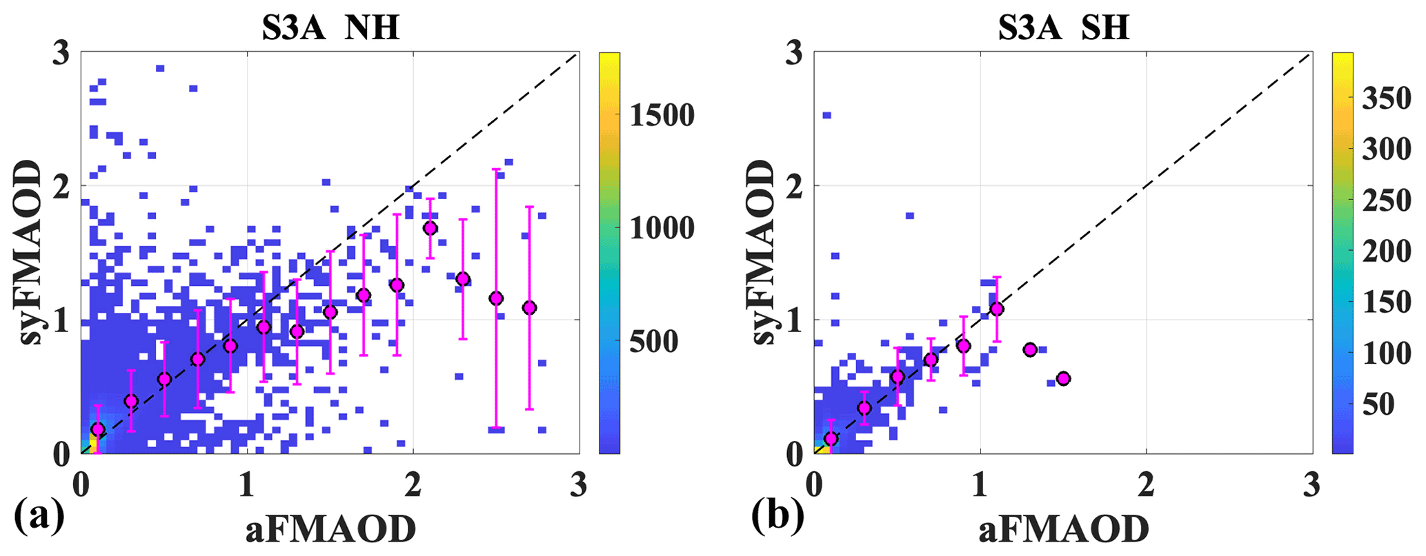
Figure 18 Density scatter plots for S3A syFMAOD and corresponding aFMAOD for collocations available over the NH (a) and SH (b).

Looking at the seasonal validation results, for both S3A and S3B, the correlation coefficient is slightly higher in MAM (0.65 and 0.67 for S3A and S3B, respectively) and JJA (0.67 and 0.69) and lower (0.56 and 0.59) in DJF (Table 2; Fig. S10, Supplement). Bias is ca. 0.1–0.12 and slightly higher (0.15 and 0.12) in JJA. The binned mean syFMAOD values are close to the 1 : 1 line for aFMAOD < 0.6–1 but fall below the line for higher aFMAOD.

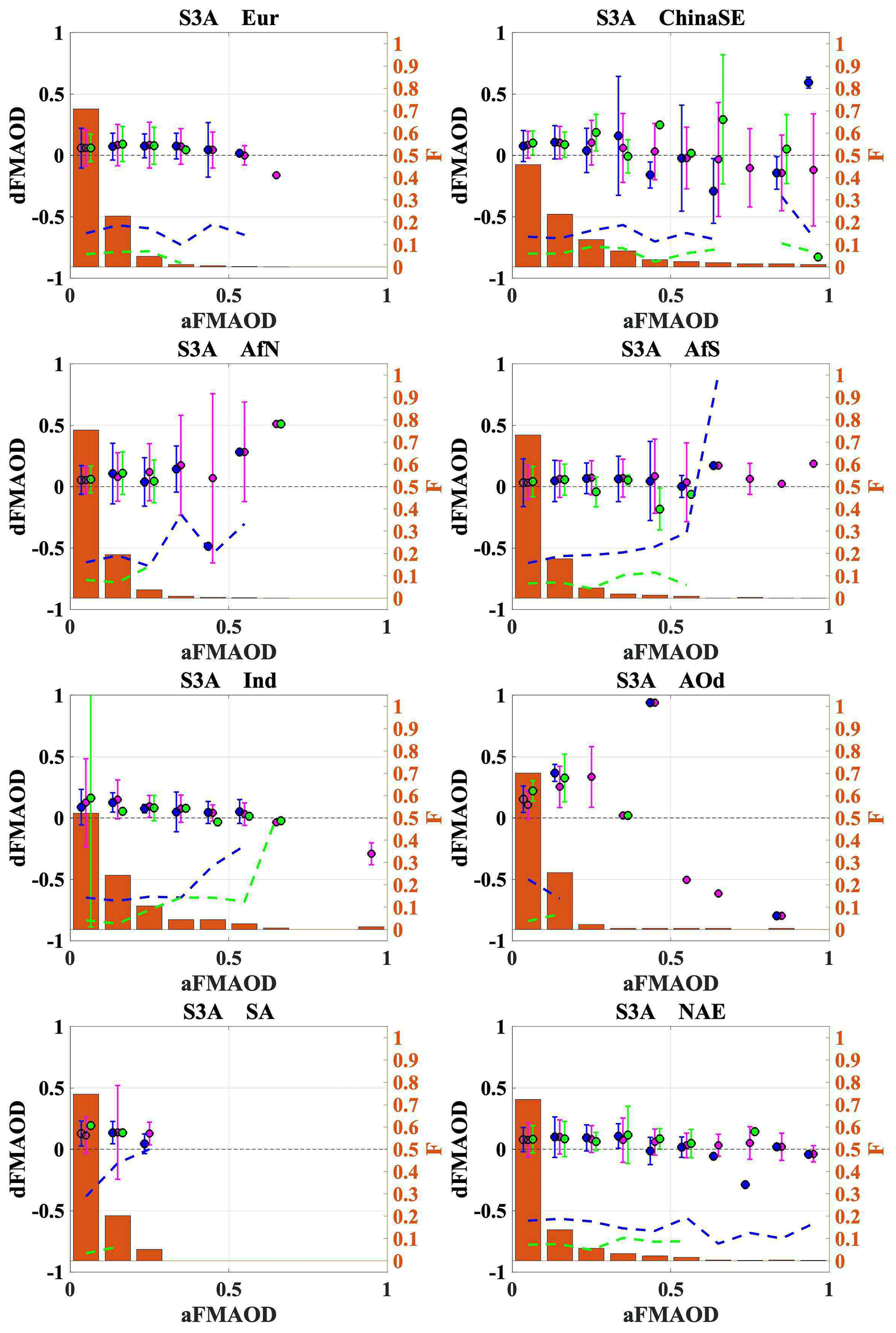
Figure 19 Regional (for Eur, ChinaSE, AfN, AfS, Ind, AOd, SA, NAE) difference (dFMAOD) between syFMAOD and aFMAOD for selected aFMAOD bins: median bias (circles) and bias standard deviation (error bars) for all AOD types (purple), aerosol fine-dominated AOD (blue) and coarse-dominated AOD (green). The fraction (F) of points in each bin from the total number of matchups is represented by orange bars. The fraction of fine-dominated matchups in each bin is shown as orange dashed-line. Results for other regions are in the Supplement (Fig. S11).

Among selected regions, offset for all aerosol types is negligible (slightly positive) in Eur, Ind, and NAW (Fig. 19). In ChinaSE and AfN, an offset increases with increasing aFMAOD over 0.5 and becomes more unstable (takes both positive and negative values).

The SY_2 fine-mode fraction (syFMF), which is a fraction of syFMAOD from the total syAOD, was validated against the AERONET fine-mode fraction (aFMF). Since syFMAOD is slightly overestimated, we expect that syFMF is overestimated as well. Density scatter plots for the relation between syFMF and aFMF in the NH and SH are shown in Fig. 20 for S3A. In both hemispheres, and thus globally, syFMF is overestimated in the aFMF range of 0–0.7; a positive offset of 0.3–0.5 at low (< 0.25) aFMF gradually decreases. At aFMF > 0.9, syFMF is slightly underestimated. Offset between syFMF and aFMF is slightly lower in the SH. For the NH and SH, R is 0.34 and 0.42, bias is 0.56 and 0.49, and slope is 0.28 and 0.37, respectively,

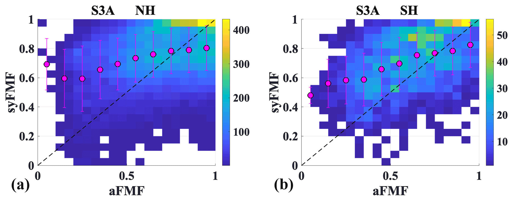
Figure 20 Density scatter plots for S3A syFMF and corresponding aFM for collocations available over the NH (a) and SH (b).

Figure 21 Density scatter plot for the difference (dFMF) between syFMF and aFMF as a function of aAOD₅₅₀. Fractions of positive (dFMF > 0.05, red line) and negative (dFMF < −0.05, blue line) overestimations per aAOD bin are shown.

A scatter density plot between dFMF (which is defined as the difference between syFMF and aFMF) and aAOD is shown in Fig. 21 for the NH and SH. In general, offset is higher at low AOD and decreases towards high AOD. The fraction of high (> 0.05) overestimates decreases towards high AOD, while the fraction of high underestimates increases.

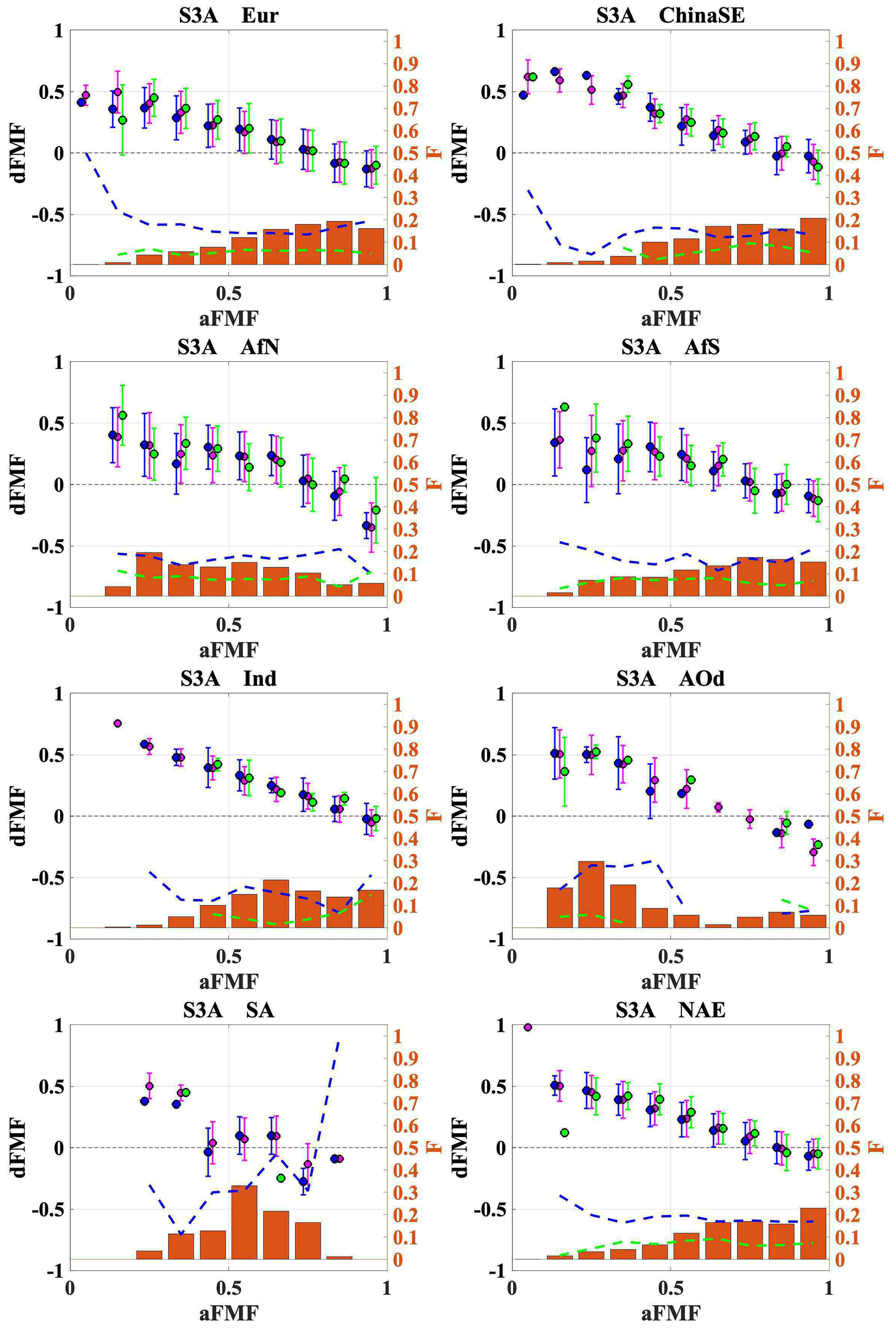
Figure 22 Regional (for Eur, ChinaSE, AfN, AfS, Ind, AOd, SA, NAE) difference (dFMF) between syFMF and aFMF for selected aFMF bins: median bias (circles) and bias standard deviation (error bars) for all AOD types (purple), as well as aerosol fine-dominated AOD (blue) and coarse-dominated AOD (green). The fraction (F) of points in each bin from the total number of matchups is represented by orange bars. The fraction of fine-dominated matchups in each bin is shown as an orange dashed line. Results for other regions are in the Supplement (Fig. S12).

Regional dFMF (Fig. 22) is positive (0.3–0.7) for low (< 0.2) aFMF and decreases gradually towards higher aFMF. At aFMF above 0.5–0.7, aFMF turns to negative (syFMF is underestimated). A similar tendency is observed for all chosen regions.

6.4 Ångström exponent

The Ångström exponent, AE, is often used as a qualitative indicator of aerosol particle size. SYNERGY AE (syAE) is calculated in the spectral interval 550–865 nm, while AERONET AE (aAE) is provided for 500–870 nm. The difference between AE_550–865 and AE_500–870 depends on the aerosol type and may be as high as 5 %–10 % of AE (personal estimations). This difference must be considered for the interpretation of the evaluation results.

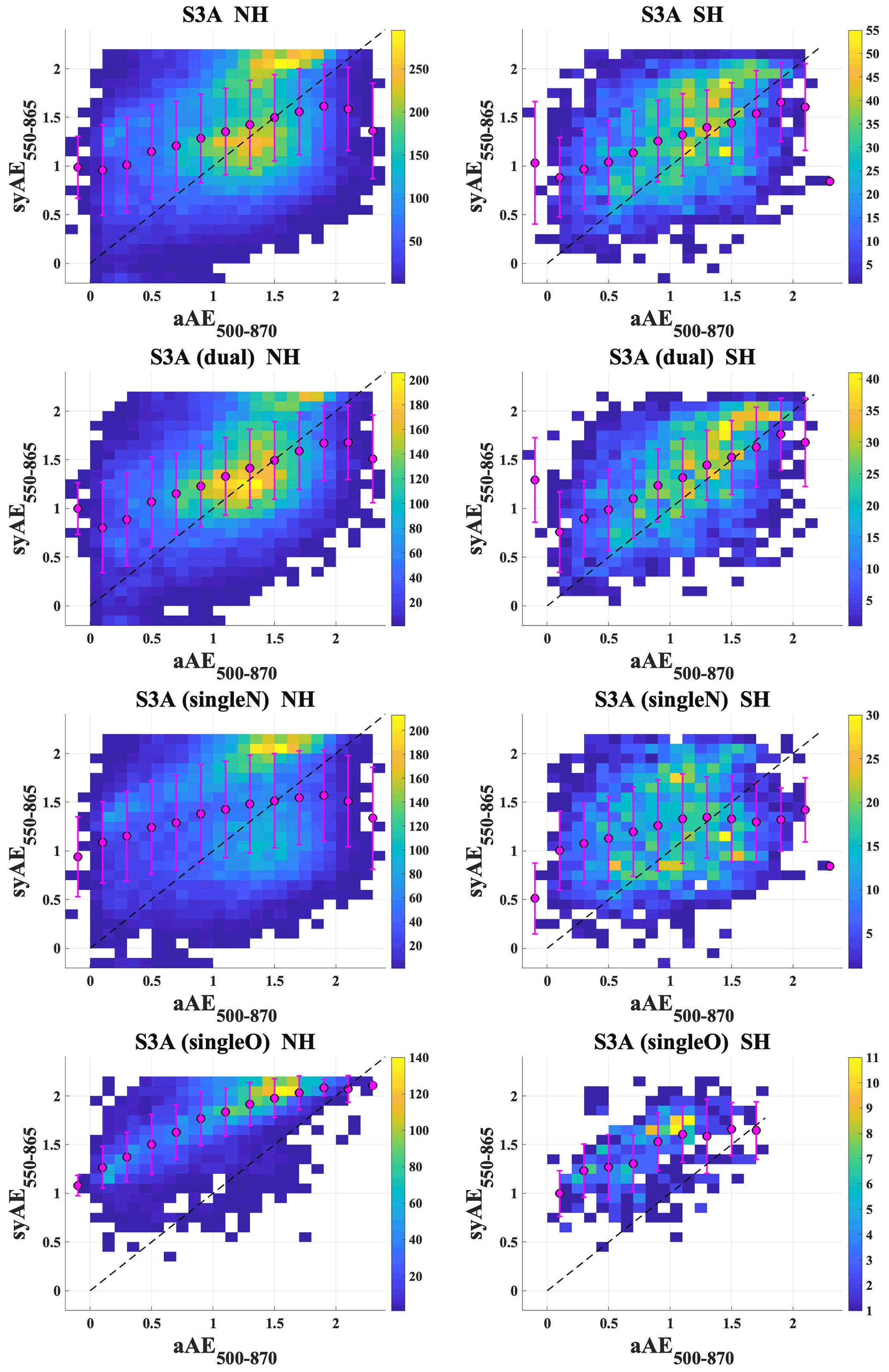
Figure 23 Scatter plots between syAE_550–865 and aAE_500–870 for S3A for the NH and SH (panels left and right, respectively) for different groups of products (top-down: all, dual, singleN, and singleO).

Scatter plots between syAE_550–865 and aAE_500–870 for S3A for all matchups and different groups of matchups are shown in Fig. 23, corresponding validation statistics are shown in Table S5 in the Supplement. Two “clouds” of satellite–AERONET AE matchups are clearly observed. The first cloud is in the aAE interval of [1, 1.6] and syAE around 1.2. In that interval, the cloud of pixels is located around the 1 : 1 line, which means that the agreement between syAE and aAE is quite good. Dual matchups contribute most to this cloud. The second cloud, formed mostly from the singleN and singleO groups of matchups, is in the aAE interval of [1.4, 1.9] and syAE around 2. In that interval, syAE is overestimated by 0.3–0.6.

For 40 % of the matchups with AERONET in the NH and for 60 % of the matchups in the SH, which fit into the aAE interval of [1, 1.8], an offset between syAE and aAE is within ±0.25. General overestimation of low (< 0.5) syAE and underestimation of high (> 1.8) syAE results in high (0.94 globally) overall bias.

For the whole global product, correlation coefficients between syAE_550–865 and aAE_500–870 are quite low at 0.35 and 0.34, and rms is high at 0.57 and 0.58 for S3A and S3B, respectively. Validation statistics are slightly better for the dual product. The singleO product shows better correlation but worse rms and SD. Validation statistics are better in the NH for all matchups and the dual product. For the single-view groups (singleN and singleO), no difference in validation results was revealed between the NH and SH.

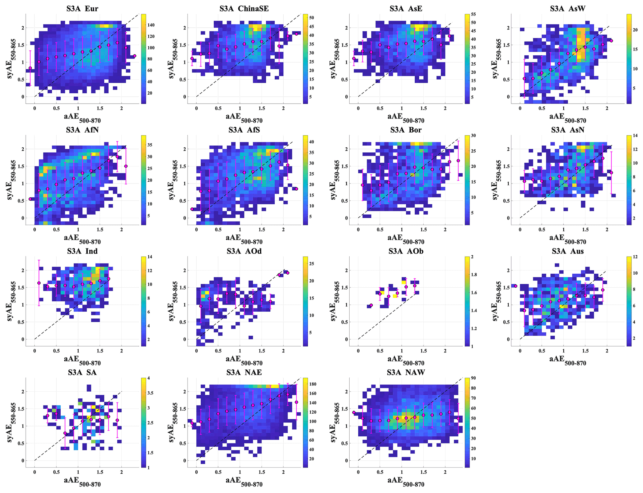
Figure 24 Regional scatter density plots between syAE_550–865 and aAE_500–870. Regions are defined in Fig. 6.

Regional analysis (Fig. 24, Table S6) reveals considerable differences in syAE evaluation results for regions with different surface type and aerosol properties. Footprints for the frequency of matchups at certain AE ranges (density value on the scatter plot) follow the “cloudy” shape in regional scatter density plots. The location of the clouds along the x axis (aAE) is specified by prevailing aerosol types in those regions. The cloudy shape of the footprint often ruins validation statistics, which should be interpreted with consideration of the matchup's footprint; see Fig. 24.

The syAE is often overestimated in the aAE range [1.3, 1.7], except for AsW, for which the fraction of good (close to the 1 : 1 line) pixels is as high as the fraction of overestimated syAOD. In AfN, low AE, which is typical for that region characterised by a high fraction of dust particles, is often highly overestimated. A dense cloud of good matchups is located near the 1 : 1 line in NAW. However, R (Table S6 in the Supplement) is low in that region because, as mentioned above, the good pixels have the shape of a cloud and statistics are defined by outliers, which are distributed evenly in all directions from the cloud. In oceanic regions with possible transport of dust aerosols, syAE is often underestimated. The low number of matchups in the AOb region (N = 22) does not allow making a solid conclusion on the syAE quality in this region.

7 Validation over ocean

Being performed aboard ships, MAN AOD measurements are irregular. S3A and S3B collocations with MAN for the period January 2020–September 2021 are shown in Fig. 25. Altogether, 105 matchups have been found for S3A and 95 matchups for S3B. Note that about half of the collocations are observed near coastal zones. Since the number of validation points is low, we show in Fig. 26 scatter plots and validation statistics for both S3A and S3B.

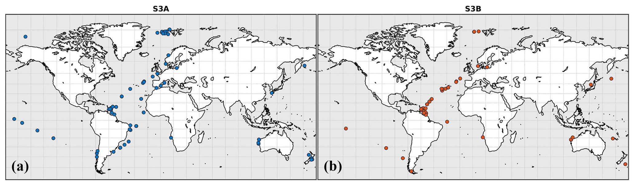
Figure 25 Collocations of S3A (a) and S3B (b) with MAN for January 2020–September 2021.

Figure 26 Scatter plots between S3A and S3B syAOD as well as MAN AOD (mAOD) with validation statistics.

Results for both instruments confirm a good performance of the retrieval algorithm over ocean. For S3A and S3B, correlation coefficients are 0.88 and 0.85, and fractions of pixels in the EE are 88.6 % and 89.5 %. An offset with MAN AOD (mAOD) is slightly higher for S3A (0.02 and 0.01), while rms is slightly higher for S3B (0.06 and 0.1).

One value from each product, S3A and S3B, can be considered a clear outlier: S3A AOD over the Baltic is underestimated, and S3B AOD over the Caribbean Sea is overestimated. The removal of these outliers from the validation exercise improves validation statistics: correlation increases to 0.95 and 0.97, rms decreases to 0.04 and 0.03, and fractions of pixels in the EE increase to 89.4 % and 92.4 % for S3A and S3B, respectively.

8 SY_2 AOD spatial performance relative to MODIS Terra DT&DB AOD product

8.1 Methods

The coverage of ground-based reference data is limited. To better evaluate the spatial distribution of the satellite-retrieved AOD, an intercomparison with other satellite products is necessary. The satellite product chosen as a “reference” must fulfil several criteria, e.g.

• i.

  overpass time as close as possible to Sentinel-3 to avoid possible different aerosol and cloud conditions;

• ii.

  wider swath (for the reference product), which allows considering most of the pixels from the tested product in the analysis;

• iii.

  similar resolution, which allows pixel-to-pixel intercomparison.

Considering these criteria, the MODIS Terra DT&DB AOD product has been chosen as a reference for evaluation of the SY_2 AOD₅₅₀ product.

The MODIS Terra DT&DB AOD product fulfils two out of the three criteria mentioned above.

• i.

  The Sentinel-3 orbit is a near-polar sun-synchronous orbit with a descending node equatorial crossing at 10:00 mean local solar time. The MODIS Terra satellite crosses the Equator on descending passes at 10:30–10:45 mean local solar time.

• ii.

  The SLSTR dual-view swath centred on the sub-satellite track is 740 km wide, with a single-view swath width of 1470 km. OLCI covers a swath width of 1270 km. MODIS Terra has a viewing swath width of 2330 km.

The third criterion is not fulfilled since MODIS and SY AOD products are provided at different resolutions. The resolution of the SY_2 product is 4.5 × 4.5 km², while the MODIS AOD daily product is available at 3 km, 10 km, and 1^∘ resolution, the MODIS monthly product is available at 1^∘ resolution. Thus, to fulfil the third criterion, we re-gridded the daily SY_2_AOD product to 1^∘ resolution for an area of interest (AOI; 30^∘ S–60^∘ N, 80^∘ W–45^∘ E) and calculated monthly aggregates. A 1^∘ grid resolution was chosen to mitigate collocation uncertainties, smooth the data, and minimise the processing time.

Two different approaches exist for evaluation and intercomparison of satellite monthly AOD. For algorithm performance intercomparison, only the spatio-temporally collocated pixels from the two products were considered (used in monthly aggregates). For climate studies (for e.g. model evaluation, trend analysis) for which existing monthly products are utilised, an intercomparison should be performed for the products built on all points available for each instrument.

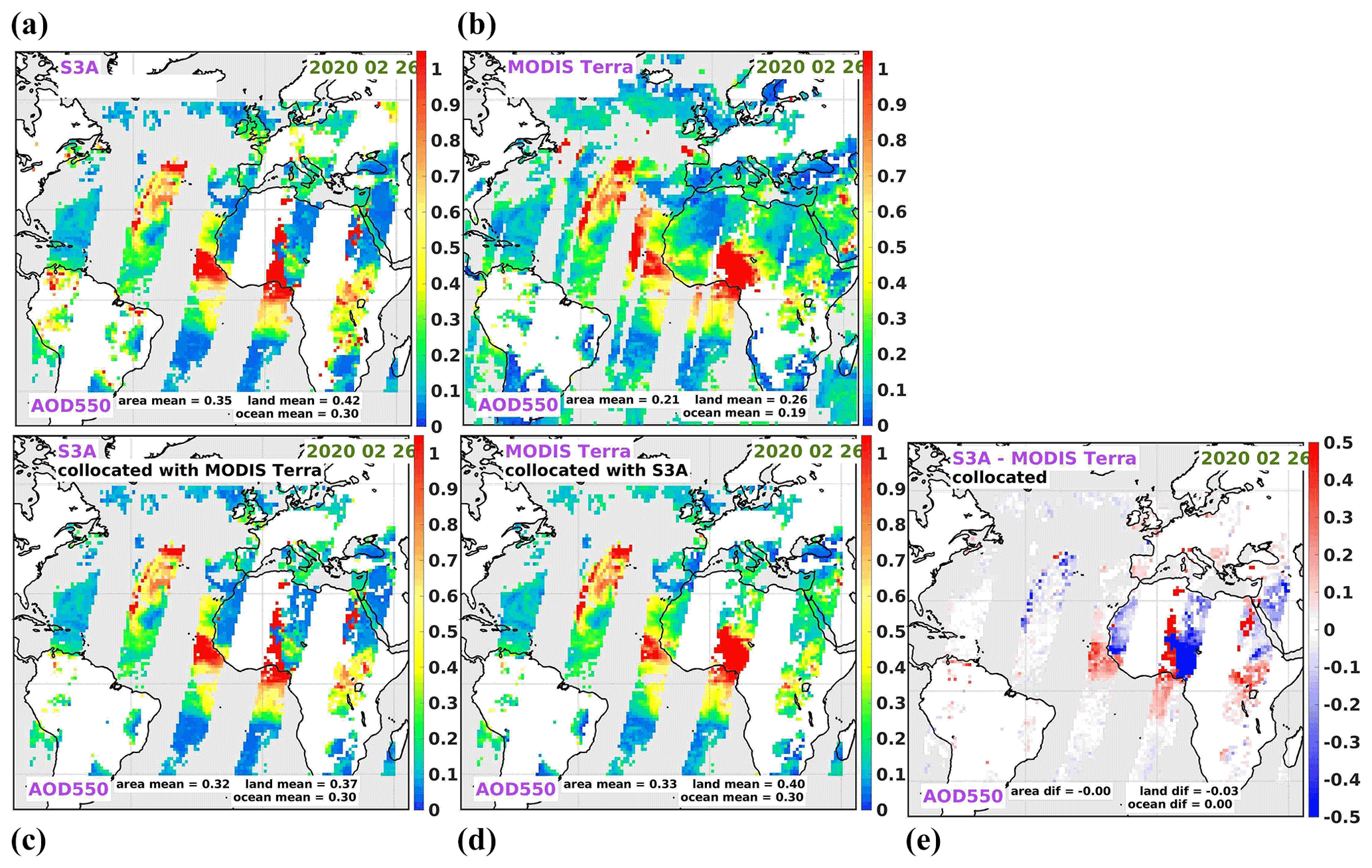
Figure 27 For 26 February 2020, all pixels available in S3A syAOD₅₅₀ (a) and MODIS modAOD₅₅₀ (b) products. Pixels existing in both products (collocated products), syAOD₅₅₀ (c) and modAOD₅₅₀ (d), as well as the difference between syAOD₅₅₀ and modAOD₅₅₀ (e). For each sub-plot, statistics (mean AOD for the whole area and separately for land and ocean) are shown.

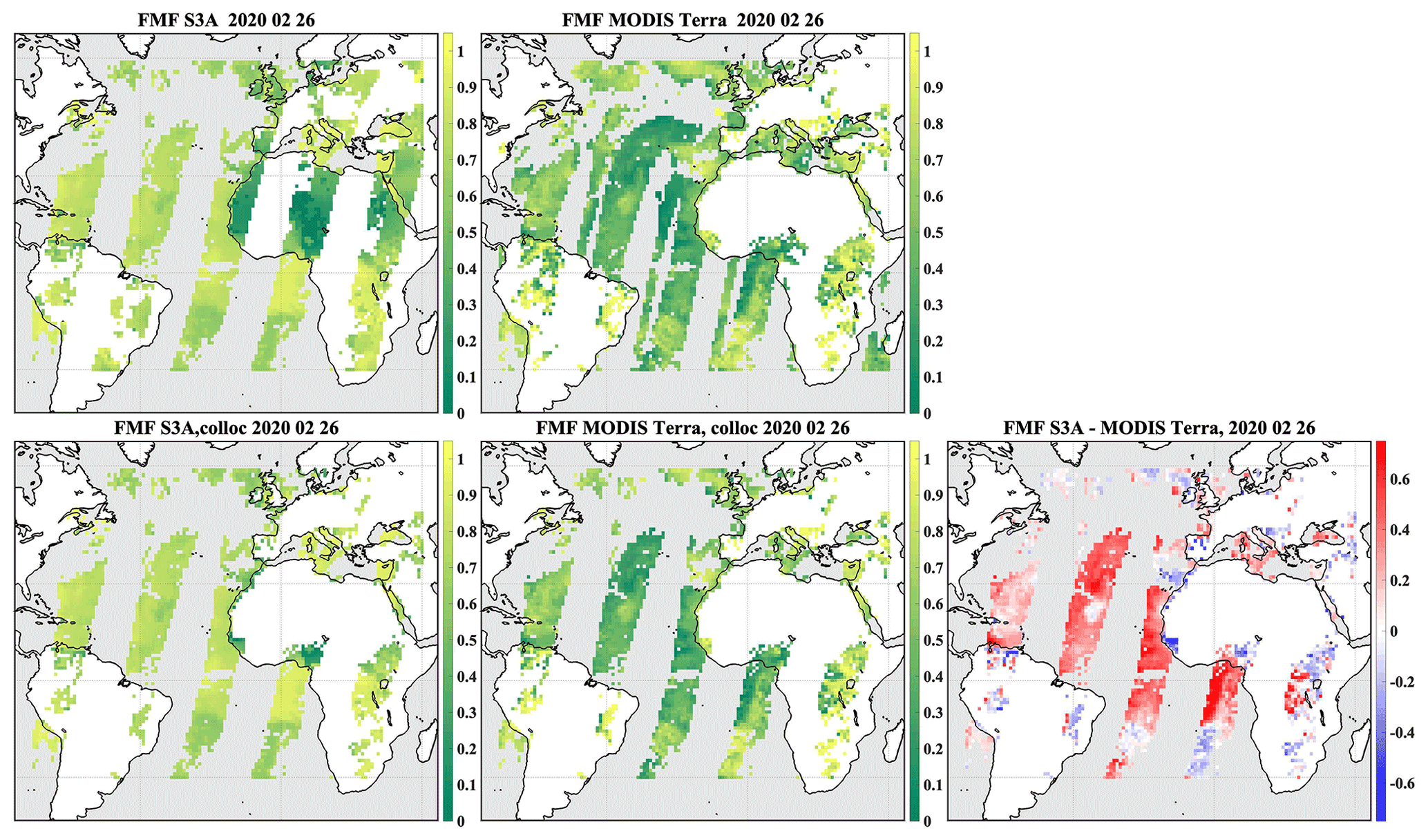
Figure 28 Same as Fig. 27 for syFMF; all pixels available in S3A FMF (a) and MODIS FMF (b) products. Pixels existing in both products (collocated products), S3A FMF (c) and MODIS FMF (d), as well as the difference between S3A and MODIS FMF (e).

SY_2 and MODIS Terra AOD products were intercompared over the area shown in Figs. 27 and 28. To evaluate and intercompare AOD products (and thus algorithm performance) in different environments (e.g. surface type, aerosol type, aerosol loading), subregions shown in Fig. 29 (top right) were chosen (see Table S7 for details).

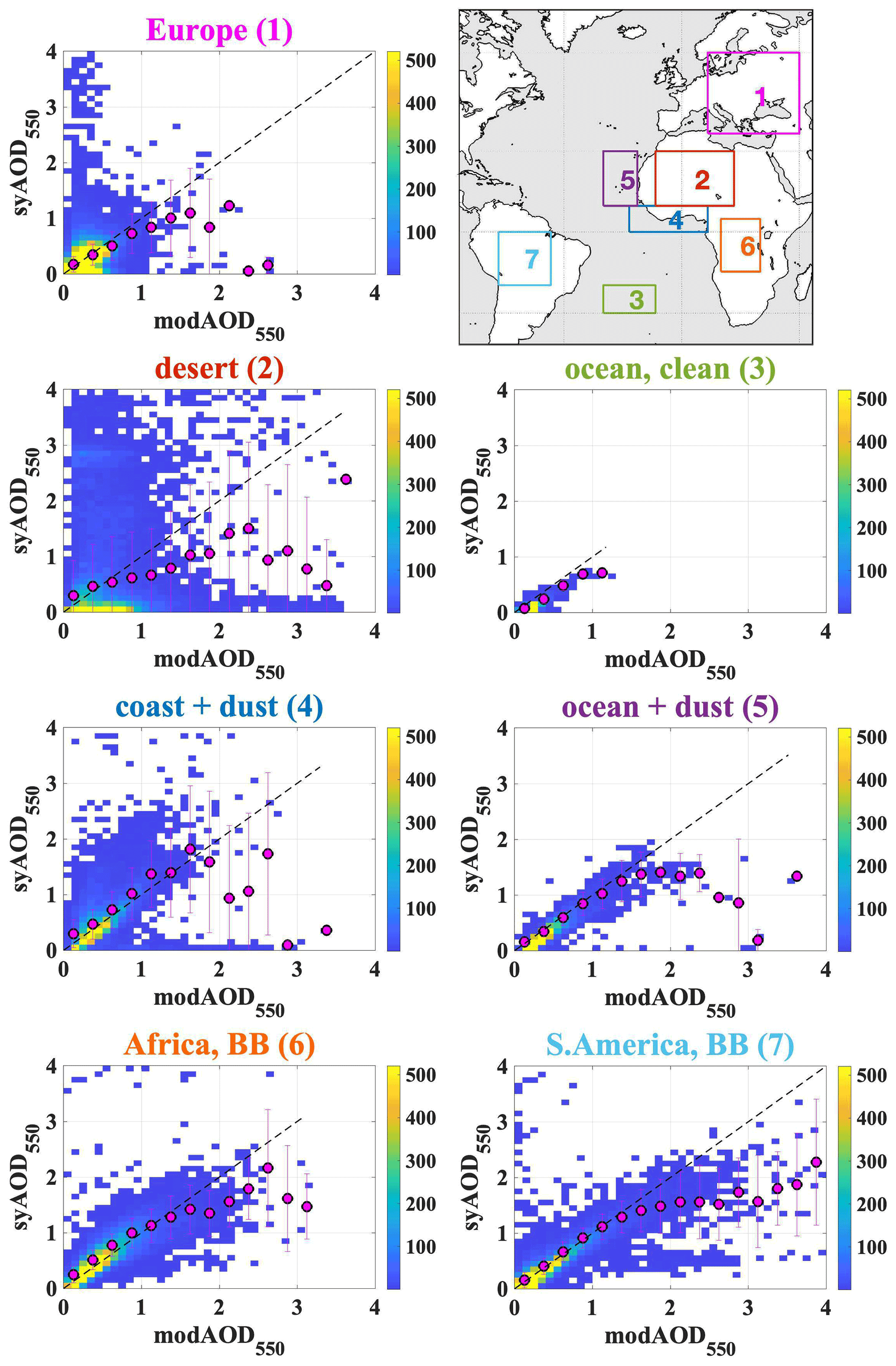
Figure 29 Density scatter plots for MODIS Terra and S3A SY_2_AOD L3 daily collocated products for 2020 for the subregions shown in the top right corner. Statistics are summarised in the Supplement (Table S9).

8.2 Intercomparison of daily AOD products

All pixels available in S3A SY_2_AOD and MODIS Terra L3 daily AOD550 products, collocated products, and differences between collocated products are shown for the whole AOI for 26 February 2020 (Fig. 27). Because of the wider swath, MODIS has larger coverage than S3A. Thus, when collocating two products for closer intercomparison, more pixels from the MODIS product are removed.

For the products containing all original pixels for each instrument, the SY_2 AOD mean over the AOI is higher than MODIS Terra AOD (0.35 and 0.21 for S3A and MODIS, respectively). Mean AOD over land and over ocean are also higher for S3A. For collocated products, mean (over the AOI) AOD for S3A and MODIS as well as AOD over ocean come very close to each other. However, SY_2 FMF (syFMF) over ocean (Fig. 28) is lower than MODIS FMF (modFMF). Also, there are regional differences mainly over a possible dust overflow over the Atlantic. MODIS provides higher AOD over the dust plume. Lower modAOD on the west of the plume may be explained by the offset between MODIS Terra and S3A overpass time. Over land, mean AOD is slightly lower for S3A for collocated pixels, and modFMF over bright surface (Sahara) is missing; over other regions the difference between syFMF and modFMF is lower compared to ocean.

For the chosen day, for S3A, a sharp transition between AOD retrieved over land and ocean at the west coast of Africa is revealed. This feature is clearly seen in the S3A and MODIS AOD difference plot. This can be explained by the land–surface gradient in the syFMF (Fig. 28). A large AOD gradient in S3A data is observed over Nigeria; the inconsistency with MODIS data reaches above ±0.5 AOD in this area. MODIS FMF is not provided in this area.

For the whole year of 2020, S3A SY_2 and MODIS AOD₅₅₀ pixel-level intercomparisons of 1^∘ × 1^∘ daily products for chosen subregions are shown as density scatter plots in Fig. 29.

In the Europe region, which includes parts of eastern and southern Europe and the Middle East, AOD is low (< 0.4) in both products in general. However, several outliers are observed in the SY_2 product (SY_2 AOD is in the range 1–4, while MODIS AOD is below 0.5). A possible reason for disagreement can be that SY_2 AOD was retrieved in cloud edge, while MODIS has been retrieving AOD in clear-sky conditions (given ca. 30 min difference between overpasses). If this is true, SY_2 cloud screening should be improved to better distinguish between aerosol and clouds in cloud edge areas. The outlier cases should be studied separately to better understand the reason for disagreement.

In the desert area the disagreement between the two products is most significant. For MODIS AOD in the range 0–0.8 most of the SY_2 pixels have AOD < 0.2, while there are also a considerable number of SY_2 pixels with AOD in the range 1–4. For MODIS AOD above 0.8, SY_2 AOD is often low, which is confirmed by bin results averaged over MODIS AOD (magenta dots in Fig. 29). The high surface reflectance typical of this area is challenging for aerosol retrieval. The large variance observed in the AOD comparison indicates that a more detailed intercomparison including the surface reflectance values retrieved by each algorithm should be performed. Over clean ocean and ocean+dust subregions, agreement between SY_2 and MODIS AOD is quite good for modAOD < 1 and modAOD < 1.8, respectively; for higher AOD, syAOD is lower than MODIS AOD.

In the coast+dust area (over which biomass burning aerosols can be transported occasionally), AOD averaged over bins is biased slightly positive for AOD < 1.2, which results from SY_2 positive outliers, while for AOD > 1.2 SY_2 AOD is often much lower than MODIS AOD, and thus binned averaged AOD is biased negative.

The footprints for SY_2 and MODIS AOD look similar in the two areas with a seasonal contribution of biomass burning aerosols (Africa,BB and S.America,BB). Agreement between SY_2 and MODIS is good for MODIS AOD below 1.2. Above that threshold, SY_2 AOD is on average lower.

Overall, the majority of data are in the low AOD range, in which agreement is decent (with SY_2 slightly high biased), but at higher AOD there is much more variance (partly due to the scarcity of data) and in general a slight low bias for SY_2.

Seasonal comparison is shown in Fig. S13 in the Supplement. Annual and seasonal statistics for SY_2 and MODIS Terra for all daily pixel AOD intercomparisons are summarised in the Supplement (Table S8).

8.3 Spatial intercomparison of seasonal and annual S3A and MODIS Terra AOD products

Two types of monthly datasets have been created from SY_2_AOD and MODIS Terra daily data to study the differences at the monthly, seasonal, and annual (MSA) level.

In the first monthly dataset, all pixels available in the SY_2_AOD and MODIS Terra daily products have been used to build a monthly aggregate for each instrument. Intercomparison of these “all-pixel” monthly aggregates (which are similar to the official monthly products provided for users) is important because it will help in e.g. understanding the difference in climate data records built from the provided monthly AOD products which include all available data.

A second monthly dataset, the “collocated” product, has been aggregated using only collocated daily pixels. Intercomparison of collocated monthly aggregates shows the difference in monthly AOD based on differences in retrieval approaches.

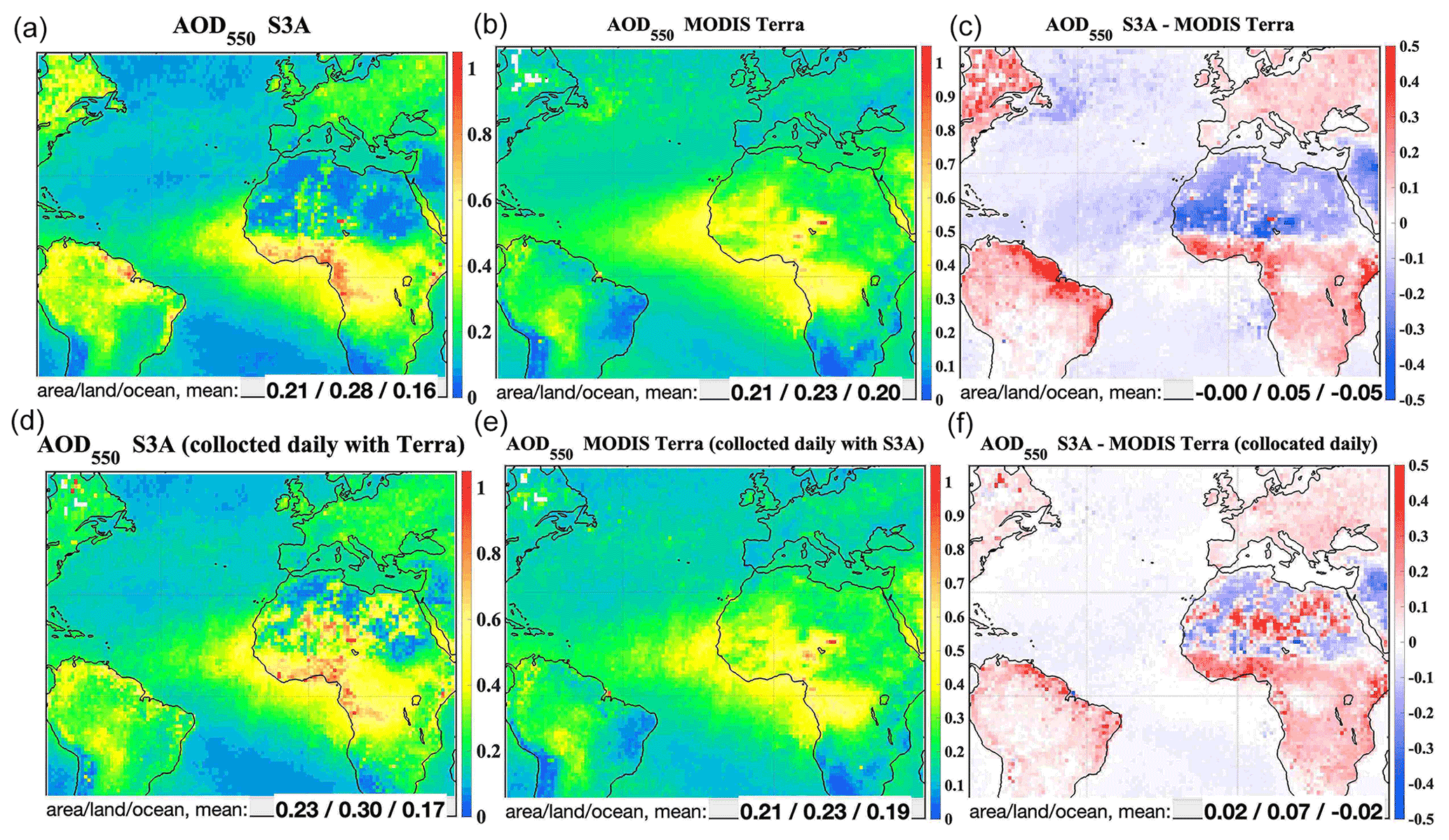
Figure 30 For the year 2020, annual S3A SY_2_AOD (a, d), MODIS Terra (b, e) AOD, and the difference between S3A and MODIS Terra (c, f) AOD. Annual means are calculated from monthly aggregates combined from all data available in each product (a–c) and pixels of collocated daily AOD (d–f). AOD mean and the difference between SY_2 and MODIS AOD for the whole area, as well as separately for land and ocean, are shown on the maps.

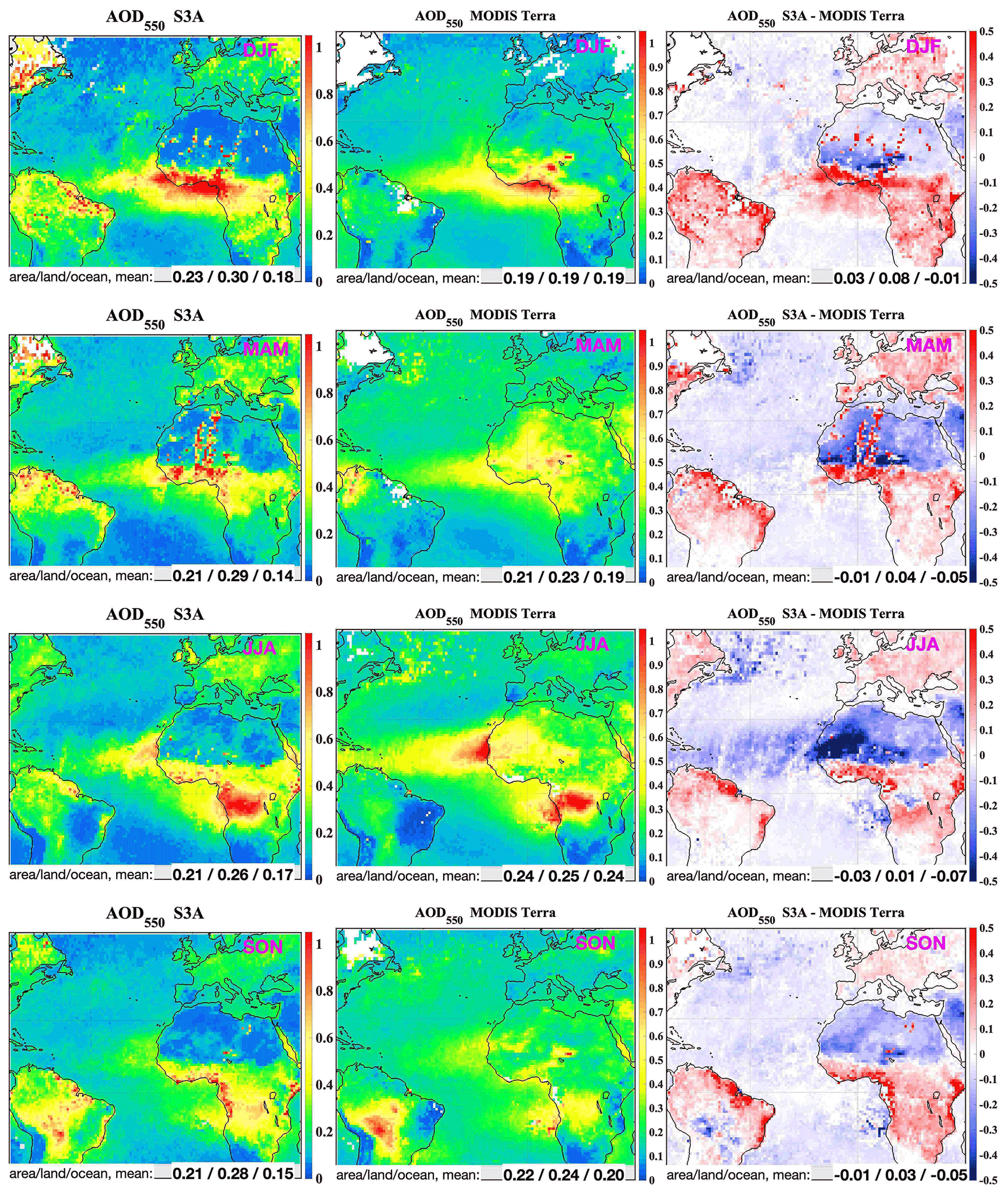
Figure 31 Seasonal (top down: DJF, MAM, JJA, SON) S3A (left panel), MODIS Terra (middle panel) AOD₅₅₀, and the difference in AOD₅₅₀ between S3A and MODIS Terra (right panel); from monthly aggregates created from collocated daily S3A and MODIS Terra AOD products.

Annual AOD from all-pixel and collocated monthly datasets for SY_2_AOD and MODIS Terra, respectively, as well as the corresponding differences are shown in Fig. 30. Seasonal plots for collocated aggregates and the difference between them are shown in Fig. 31. Statistics for difference plots (area, land, and ocean means) have been calculated from pixel-to-pixel difference, but not as the difference between the AOD averaged over AOI, land, and ocean.

Differences between SY_2_AOD and MODIS Terra MSA AOD exist in both the all-pixel and collocated datasets. For both datasets, SY_2 AOD averaged over AOI is higher for the whole area, as well as for land and ocean. The difference is smoother for the all-pixel datasets. Even though difference plots show that regional offset between the two datasets is often within GCOS requirements for AOD quality (0.03) over ocean (SY_2 AOD is in general lower) and the whole AOI, the difference in AOD over land is often higher (up to 0.11 as averaged over AOI in DJF, all-pixel dataset).

Regional differences in seasonal AOD from the collocated dataset are considerably higher (Fig. 31). For all land subregions (except for “desert”, JJA), S3A AOD is higher than MODIS AOD. The offset is highest for the “coast+dust” region in DJF and for the “Africa,BB” region in SON (0.18 and 0.15, respectively). A general tendency of decreasing offset towards JJA months has been observed. However, though the offset is often high, time series for both products are within an overlap (grey area) of the standard deviations for individual products. The highest negative offset (between 0.05 and 0.1) is observed in JJA in the desert region. Regional differences in seasonal AOD from the all-pixel dataset are less scattered (Fig. S14, Supplement).

For the open-ocean regions (“ocean, clean”, and “ocean+dust”), S3A AOD is in general lower than MODIS AOD for all MSA; the exceptions are January and February in the ocean+dust region (Figures not shown). On the annual scale, the offset between S3A and MODIS AOD is −0.02 for ocean+dust and −0.03 for ocean and clean. AOD in the collocated dataset is higher compared to the all-pixel dataset for both S3A SY_2 and MODIS Terra. Comparing with all pixels and collocated, the SY_2 AOD product looks less smooth over northern Africa in DJF and MAM.

9 Conclusions and recommendations for future evolution

We have presented the first validation of a new SYNERGY global aerosol product, derived from the data from the OLCI and SLSTR sensors aboard the Sentinel-3A and Sentinel-3B satellites. Combined, the two satellites provide close to daily global coverage and provide aerosol measurements with a latency of 2–3 d. In this study we have compared the aerosol product with ground-based photometer data from four networks: AERONET, SKYNET, SURFRAD, and MAN, as well as with MODIS combined Dark Target and Deep Blue algorithms. The aim of this study was to provide global characterisation of the current aerosol retrieval and to guide future algorithm development.

Over ocean, the performance of SYNERGY-retrieved AOD is good and consistent with the reference MAN dataset (rms ∼ 0.05), although the MAN validation has a limited set of higher-AOD examples. Against MODIS, agreement is good, although SYNERGY AOD shows lower values at high AOD (> 1.5) in dust regions, potentially indicating that cloud screening improvement is needed to correctly detect high dust levels.

Over land, overall performance has a much higher rms error of approximately 0.25 when compared to AERONET. Overall AERONET correlation is ∼ 0.6. Reduced performance over land is expected since the surface reflectance and angular distribution of scattering are higher, and they are more difficult to treat over land than over ocean. However, the results show that these statistics are affected by a large number of outliers. Inspection of these outliers and patterns of disagreement with MODIS indicate possible reasons and targets for future algorithm evolution. The main causes are (i) poor screening of snow- and/or ice-covered surfaces and (ii) inadequate cloud screening in some regions. For example, in tropical forest areas, care needs to be taken to fully exclude any pixels containing clouds, including sub-pixel clouds in either nadir or oblique view. In addition, removal of cloud edge pixels (cloud-free pixels next to cloud-masked pixels) should be considered. Bright desert surfaces also have less stable retrieval, with land–ocean contrast suggesting that high values in dust plumes are underestimated over land. Further uncertainty is introduced by an error in a priori estimates of aerosol properties not retrieved, principally single-scattering albedo (SSA).

It is clear that retrievals using dual view give higher quality by making use of more information to allow less reliance on surface spectral assumptions. Retrieval over land surface in the Northern Hemisphere shows generally higher retrieval error, including regions of boreal forest where we would expect higher-quality retrieval due to the low surface signal. In some cases, this will be due to weak masking of snow and ice cover as well as the presence of retrievals made at high solar zenith angles (over 70^∘) often excluded in other aerosol datasets. In addition, since the land retrieval relies on use of the oblique SLSTR view we expect to see higher-quality retrievals in the SH compared to NH. This is due mainly to sampling of backscattered light by the SLSTR oblique view in NH, where aerosol has a weak signal and the surface signal is higher, while in SH the geometry is reversed. Over ocean this is not the case, as the retrieval is not reliant on the oblique view, and indeed the geometry results in less sunglint in NH ocean.

The retrieval of the Angström exponent, related to aerosol size distribution, shows spatial correlation with expected sources but generally overestimates AE for cases in which AERONET Angström is low, resulting in overall high bias. This is dependent on the retrieval of the fine-mode fraction in the algorithm, which needs to be investigated further and improved. Evaluation of the per-retrieval uncertainty indicated good correlation with measured error distributions, with overprediction of expected error in the dual-view case and underprediction in the single-view case. Evaluation of the uncertainty propagation is difficult in the presence of outliers which do not fit the algorithm assumptions, for which we see a tail of higher errors, for example related to undetected cloud in the input data.