the Creative Commons Attribution 4.0 License.
the Creative Commons Attribution 4.0 License.
 | 26 Sep 2022
Ozone reactivity measurement of biogenic volatile organic compound emissions
Detlev Helmig
Alex Guenther
Jacques Hueber
Ryan Daly
Jeong-Hoo Park
Anssi Liikanen
Arnaud P. Praplan
Previous research on atmospheric chemistry in the forest environment has shown that the total reactivity from biogenic volatile organic compound (BVOC) emissions is not well considered in forest chemistry models. One possible explanation for this discrepancy is the unawareness and neglect of reactive biogenic emissions that have eluded common monitoring methods. This question motivated the development of a total ozone reactivity monitor (TORM) for the direct determination of the reactivity of foliage emissions. Emission samples drawn from a vegetation branch enclosure experiment are mixed with a known and controlled amount of ozone (resulting in, e.g., 100 ppb of ozone) and directed through a temperature-controlled glass flow reactor to allow reactive biogenic emissions to react with ozone during the approximately 2 min residence time in the reactor. The ozone reactivity is determined from the difference in the ozone mole fraction before and after the reaction vessel. An inherent challenge of the experiment is the influence of changing water vapor in the sample air on the ozone signal. Sample air was drawn through Nafion dryers to mitigate the water vapor interference, and a commercial UV absorption ozone monitor was modified to directly determine the ozone differential with one instrument. These two modifications significantly reduced interferences from water vapor and errors associated with the determination of the reacted ozone as the difference from two individual measurements, resulting in a much improved and sensitive determination of the ozone reactivity. This paper provides a detailed description of the measurement design, the instrument apparatus, and its characterization. Examples and results from field deployments demonstrate the applicability and usefulness of the TORM.
- Article
(1633 KB) - Full-text XML
-
Supplement
(1111 KB) - BibTeX
- EndNote


Recent field research on the atmospheric chemistry in forest environments has yielded a series of results that cannot be explained with our current comprehension of biogenic emissions, deposition processes, and chemical reactions. These findings date back to the pivotal paper by Di Carlo et al. (2004) that stimulated new interest and research in the question of unaccounted for biogenic volatile organic compound (BVOC) emissions. These researchers compared the directly measured hydroxyl radical (OH) reactivity in ambient air at the University of Michigan Biological Station (UMBS) PROPHET forest research site with the OH reactivity calculated from a comprehensive set of measured atmospheric gas-phase species. The important conclusion of this study was that identified compounds could only account for about of the directly measured OH reactivity. Interestingly, the difference between the two measurements, often called “missing OH reactivity”, showed a temperature dependence similar to that found for monoterpene (MT) compounds. This similarity led the authors to hypothesize that the missing OH reactivity is due to non-identified BVOC emissions from tree foliage at this site.
While these findings were surprising at the time of publication, several other subsequent studies have come to similar conclusions. OH reactivity measurements in ambient air have consistently shown higher OH reactivity values than what can be accounted for by quantified chemical species, and notably, the review of available measurements shows a tendency towards a higher discrepancy at sites that are subjected to a relatively high influence from BVOC emissions (Lou et al., 2010).
The other line of research that has pointed towards the current underestimation of BVOC emissions relies on ozone flux observation over forest canopies. Kurpius and Goldstein (2003) segregated ozone deposition fluxes over a ponderosa pine plantation into stomatal uptake, non-stomatal surface deposition, and gas-phase chemistry contributions. They found that during summer, the ozone flux was dominated by gas-phase chemistry and that the ozone loss showed an exponential increase with temperature, with similar behavior as BVOC emissions. However, identified BVOCs could only account for a small fraction of this reactivity. Consequently, these researchers postulated that there is a “large unrecognized source of reactive compounds in forested environments”. A follow-up study (Goldstein et al., 2004), based on measurements during a forest-thinning experiment, went even further and claimed that “unmeasured BVOC emissions are approximately 10 times the measured monoterpene flux”. These hypotheses have been supported by findings from a series of other subsequent studies (Altimir et al., 2004, 2006; Holzinger et al., 2005; Hogg et al., 2007; Fares et al., 2010a, b, c; Wolfe et al., 2011).
There has been considerable progress in identifying and characterizing hitherto unrecognized BVOC emissions. The most significant ones are light-dependent MT emissions (Ortega et al., 2007; McKinney et al., 2011) and sesquiterpenes (SQT) (Duhl et al., 2008). Furthermore, it has been recognized that methyl chavicol can be a significant emission (Bouvier-Brown et al., 2009a, b; Misztal et al., 2010). However, inclusion of these emissions only contributes a minor fraction to closing the gap between identified and inferred BVOC concentrations. In a study at the PROPHET site, using the comparative reactivity method, Kim et al. (2011) directly determined the OH reactivity in emission samples drawn from branch enclosures. OH reactivity was also calculated based on BVOC emissions identified by proton transfer reaction mass spectrometry (PTR-MS) and gas chromatography mass spectrometry (GC-MS). A red oak, white pine, beech, and maple tree were investigated. Their results indicated a high range of total OH reactivity from the emissions of these species, with red oak emissions showing the highest OH reactivity overall. Identified isoprene and MT emissions could explain the directly measured OH reactivity from red oak, white pine, and beech. However, isoprene and monoterpene emissions from red maple could only explain a fraction of the measured OH reactivity. The OH reactivity from maple was dominated by emission of the SQT α-farnesene, which is a compound that had not been identified in earlier studies of ambient BVOCs at this site. These findings show that the chemical reactivity in emissions from different tree species can vary substantially in their overall magnitude and attribution to the emitted BVOC species. This indicates that there is the potential that ecosystems with different plant species composition could have substantial unaccounted for emissions that contribute to OH reactivity. This suggests that there must be BVOCs or compound classes emitted from foliage that current measurements do not capture, which is not unexpected given the major analytical challenges associated with analysis of some organic compounds.
In this work, we are describing a monitoring approach that addresses this dilemma by constraining the total ozone reactivity of BVOC emissions with a direct measurement. These observations can be contrasted with the reactivity that is calculated from the sum of the reactivities of individual BVOCs and their OH reaction rates to assess the fraction of the identified and missing compounds that contribute to the total reactivity. The instrument relies on a flow reactor. Sample air containing BVOCs is mixed with a small flow containing a high mole fraction of ozone. The loss of ozone is monitored with a differential ozone measurement. The total ozone reactivity monitor (TORM) that was previously presented (Helmig et al., 2010; Park et al., 2013) has since undergone further testing and development. The calculation of ozone reactivity is explained in Supplement Sect. A, and the modeled decay of a few typically measured BVOCs and ozone in the reactor is available in Supplement Sect. B.
Two other instruments relying on different types of reactors and detection methodologies have been reported since (Matsumoto, 2014; Sommariva et al., 2020). These publications have also provided the principle and reaction kinetics consideration for this measurement. A linear double-tube Pyrex glass tube flow reactor with ozone detection upstream and downstream of the reactor by two modified commercial (ECO PHYSICS, CLD770) chemiluminescence detectors (CLDs) was used in the work by Matsumoto (2014). The ozone reactivity was determined from the difference of the two analyzers' signal. A 1 m long, 2.4 L volume polytetrafluoroethylene (PTFE) linear reactor was used by Sommariva et al. (2020). These authors used two commercial Thermo Scientific model 49i UV absorption monitors for the ozone determination, with the ozone reactivity again determined from the difference of the two monitor signals.
We particularly emphasize the necessity of properly characterizing the interference from water vapor with the ozone determination and the advantage of the measurement of the amount of reacted ozone through differential ozone determination with a single monitor. Thirdly, using readily available instrument components facilitates relatively easy, low-expense instrument assembly.
Rigid chambers or flexible bag enclosures are the common approaches for studying biogenic emissions by dynamic or static vegetation enclosures (Ortega and Helmig, 2008; Ortega et al., 2008). Enclosure experiments allow the selective identification of emissions from individual plant species. Depending on the operational parameters, emissions can build up to many times, even order of magnitudes, higher levels than in ambient air. Higher temperatures (than in ambient air) are often encountered inside enclosures from the greenhouse warming effect, which enhances emissions and facilitates higher sensitivity of emissions determination. An inherent disadvantage and analytical challenge, however, is the evaporative water flux from the transpiring enclosed foliage. Under the most extreme and not too uncommon conditions, water vapor saturation can be achieved inside the chamber, causing liquid water condensation on the chamber inside walls and within sampling tubing. The water flux is sensitive to the stomatal conductance, responding to conditions of light and temperature. In an ambient setting, these often change dynamically, causing similarly fast changes in water vapor concentration inside the enclosure and sample air. At 30 ∘C and water saturation, the water vapor mole fraction is approximately 4.2 %. A mere 10 % fluctuation equates to 4.2 parts per thousand (‰) or 4 200 000 ppb of a water vapor change. The signals that have been achieved in ozone reactivity monitoring instruments system are usually in the single parts per billion range for Δ[O3]. Consequently, for the ozone monitoring to be selective, the ozone detection needs to be insensitive to water vapor changes that can be on the order of 106–107 times larger in mole fraction than the ozone signal. This is an enormous challenge for this measurement, as both the ozone CLD and UV absorption measurements are sensitive to water vapor.
Interference with an instrument signal response in the range of tens to hundreds of parts per billion has been reported for different types of UV absorption monitors from rapid changes in water vapor (Wilson and Birks, 2006; Spicer et al., 2010). This interference was traced to humidity effects on the transmission of light, i.e., reflectivity of light on the cell walls, through the optical cell (Wilson and Birks, 2006). The study identified the instrument's ozone scrubber as amplifying this effect, acting as a water reservoir by adding or removing water to the airflow depending on the sample air moisture content. A 10 % change in the recorded ozone was observed from a 30 % to 80 % relative humidity (RH) increase for a UV absorption monitor in other studies (Kim et al., 2019, 2020). Inserting a Nafion dryer into the sampling path can reduce the water interference, in the best scenario equal to or better than ± 2 ppb (Wilson and Birks, 2006; Spicer et al., 2010; Kim et al., 2020). Sommariva et al. (2020) found that the ozone wall losses were dependent on the relative humidity in their PTFE flow reactor.
While CLD analyzers for ozone determination are more expensive to acquire and operate, they are popular for fast ozone measurements such as for aircraft (Ridley et al., 1992) and eddy covariance flux measurements (Lenschow et al., 1981, 1982). Similarly to UV monitors, CLD instruments suffer from interference by water vapor, which in this case is caused by the quenching of the chemiluminescence signal in the reaction chamber (Matthews et al., 1977; Boylan et al., 2014). A correction factor of 4–5 × 10⁻³ has been proposed, to be multiplied by the water vapor mole fraction in nmol mol−1 (Boylan et al., 2014). Under moist ambient air conditions, this correction can account for up to 15 % of the ozone signal. Consequently, following the enclosure system water vapor estimates above, CLD in an ozone reactivity system may be susceptible to several percent of interference from changing water vapor, which is on the same order of magnitude as the ozone reactivity observed in the flow chamber system.
Both Matsumoto (2014) and Sommariva et al. (2020) used two ozone monitors for determination of the ozone upstream and downstream of the reactor, with the reacted ozone then determined as the difference of the recordings from both instruments. One objective of this configuration in the Matsumoto (2014) work was to achieve a reduction of the quenching interference based on the assumption that both monitors would have similar responses to the water interferences, with these errors then mostly canceling out in the differential ozone reactivity signal calculation. From a measurement and signal perspective, this is a rather disadvantageous measurement approach for several reasons: (1) the two monitors need to be carefully synced and calibrated against each other to make sure the instrument offset is characterized and corrected for so that their readings are consistent; (2) drifts of any of the two monitors, or of both, will directly transfer to a measurement error in Δ[O3]; and, (3) statistically, the calculation of the ozone reactivity will be subject to a relatively large error, as the differential signal is a relatively small value resulting from the difference between two larger numbers. Any absolute errors in the directly measured values will therefore transfer into a relatively large error of the smaller differential. For these reasons, it would be preferable to measure the ozone differential through a direct measurement with one monitor. Furthermore, a one-monitor measurement would be advantageous in terms of instrument maintenance and cost.
Our experiment presented here overcomes this predicament by modifying a commercial UV absorption ozone monitor for the direct measurement of the ozone differential. Further, sample drying was implemented to reduce the aforementioned interference from fluctuations in the sample water vapor mole fraction. The experiments were conducted on two similar systems. The first instrument was developed at the University of Colorado, Boulder (CU). Colleagues from the Finnish Meteorological Institute (FMI) in Helsinki visited CU for collaborative research on the experiment and then constructed a similar instrument to be used for their research at FMI. Both groups subsequently collaborated on further characterization and improvements of the TORM and on an Arctic field deployment. In this paper, unless otherwise noted, we report experimental results from the CU instrument. In cases in which results from the FMI instrument are reported, those are identified as FMI data. Experimental results from the CU and FMI instruments were compared throughout the instrument development. The comparison of results and the consistency in performance between the two instruments can be considered further evidence for the reproducibility of the TORM performance.
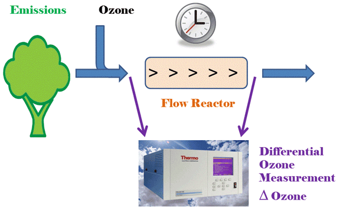
Figure 1Principle of the ozone reactivity measurement of biogenic emissions with one monitor that is configured for differential ozone signal recording.
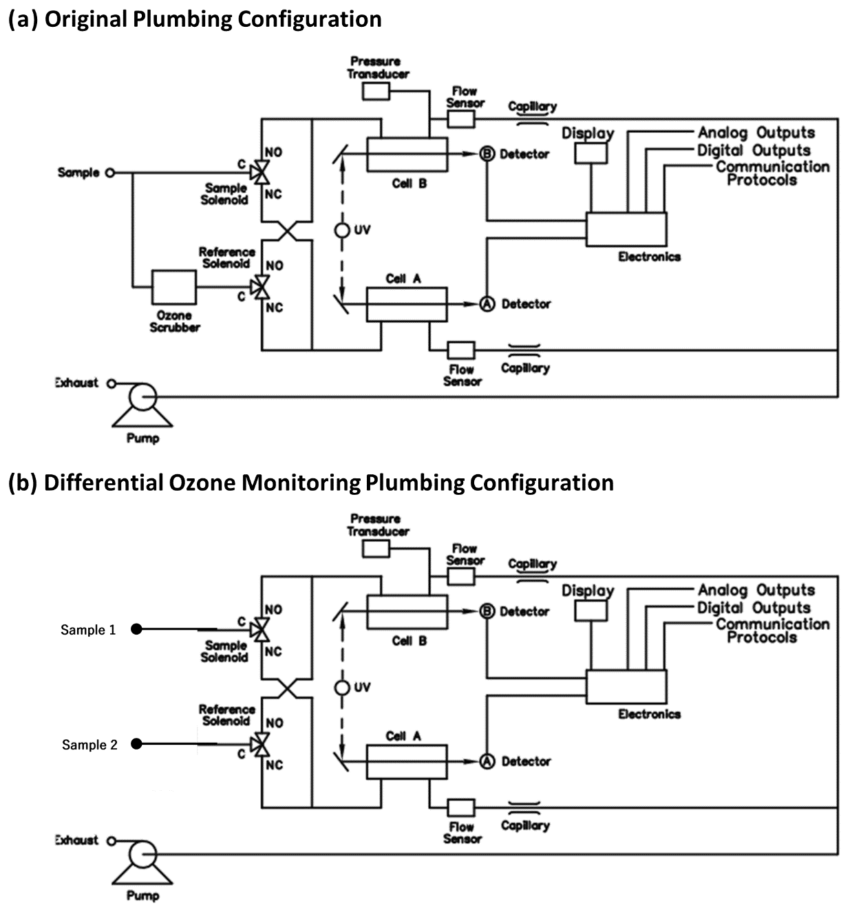
Figure 2Plumbing of a Thermo Scientific Instruments model 49 ozone UV absorption monitor in its original configuration (a) and in the modified configuration (b) for the direct monitoring of ozone differentials.
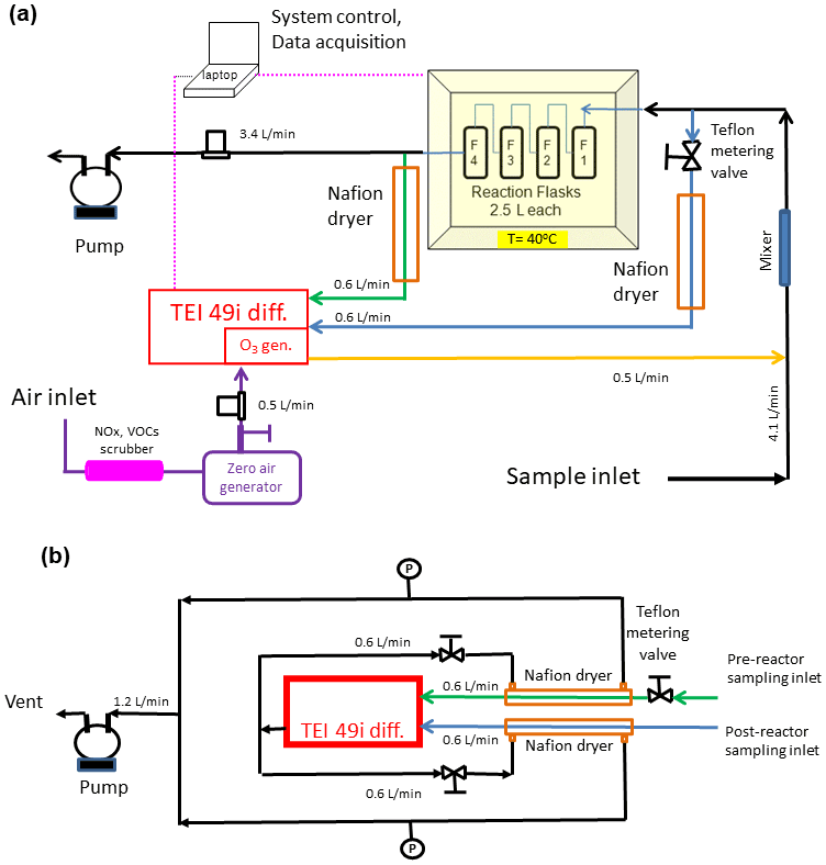
Figure 3(a) Final configuration of the total ozone reactivity analyzer (TORM) using one Thermo Scientific (TEI) 49i PS monitor plumbed for the direct differential ozone measurement (Fig. 2) as well as with the Nafion dryers and metering valve included. Flow rates are indicated in the figure. Total flow through the reactor is 4 L min−1. Please note that for simplicity this drawing does not show a second ozone monitor that was used for sampling the inflowing air between the mixer and the reactor to measure the ozone going into the reactor and setting the proper ozone output of the TEI 49i ozone generator. (b) Detail of the Nafion dryer plumbing including the external pump that was added to the system to provide the purge flow for the Nafion dryers.
The basic principle of the ozone reactivity determination of biogenic emissions is illustrated in Fig. 1. Emissions from vegetation are combined with a flow of ozone-enriched air and allowed to react in a flow reactor. Ozone is measured upstream and downstream of the reactor with a single instrument. In the standard configuration of a UV absorption ozone monitor, ozone-containing air and scrubbed air (ozone-free air) are either measured sequentially (one optical cell) or in parallel (two cell instruments), with the ozone mole fraction then determined following the Beer–Lambert law. The ozone mole fraction is proportional to the natural logarithm of the light intensity I divided from the sample air (flow 1) by the light intensity in the scrubbed air Io (flow 2). By replacing the scrubbed airflow path with a second sampling inlet line, the resulting signal no longer reflects the difference in ozone between the sample (1) and scrubbed air (2, zero ozone) but instead becomes the difference in ozone between the two sample flows (2–1). The required instrument modification is rather simple and is illustrated in Fig. 2 for a Thermo Scientific Model 49i instrument. It requires removal of the ozone scrubber (MoO scrubber in most cases) and the separation of the scrubbed and sample airflows into two separate inlets. In the standard configuration, the 49i samples air at ≈ 1.2 L min−1 through one inlet. In the modified configuration, this flow is split in half to ≈ 0.6 L min−1 each for the Sample 1 and Sample 2 inlets. An early configuration of the experiment to illustrate how the differential ozone monitoring was evaluated against the monitoring of ozone upstream and downstream of the reactor with two instruments is presented in Supplement Sect. C; the final one-monitor TORM configuration is shown in Fig. 3a. The direct differential ozone measurement was always conducted with a Thermo Scientific model 49i monitor. During the evaluation experiments, several different UV absorption ozone monitors were used for comparing the direct measurement with a result from two individual instruments. Those included Thermo Scientific model 49i and model 49C instruments, as well as a MonitorLabs model 8810 monitor. The ozone that was added upstream of the reactor was generated by the Thermo Scientific 49i instrument (with ozone generator option) to yield a target ozone mole fraction of 100 ppb. To determine the proper ozone output from the generator, an additional ozone monitor temporarily sampled the air downstream of the mixer. The ozone monitor was removed after dialling the ozone output to the target level, monitoring it for several days, and ensuring its constant output.

Figure 4(a) Photograph of one of the glass flasks that were used for the University of Colorado flow reactor. (b) The ozone reactor with four of the flasks plumbed in series contained in an insulated and temperature-controlled field-deployable enclosure. Four flasks were plumbed in series for a total flow reactor volume of 10 L. (c) The 2 L bottles (borosilicate glass 3.3) used in the flow reactor system from FMI.
While other studies (Matsumoto, 2014; Sommariva et al., 2020) utilized linear flow reactors, this experiment relied on using four glass flasks that were plumbed in series. The glass flask reactor design was chosen because it was deemed more compact and robust for field deployment applications. The 2.5 L borosilicate flasks that were used are air sampling flasks that are routinely deployed in the NOAA Cooperate Sampling Network for the global sampling of greenhouse gases. These glass flasks have been developed and extensively tested for their inertness and purity towards atmospheric trace gases (https://gml.noaa.gov/ccgg/flask.html, last access: 5 August 2022; flasks are fabricated by Allen Scientific, Boulder, CO). Flasks are covered with shrink tubing as a protective film (polyolefin shrink wrap, https://buyheatshrink.com, last access: 5 August 2022) and have two ports with stopcock Teflon vales. The valve in the center of the flask (Fig. 4) connects to a dip tube that leads to the inside and the opposite end of the flask. This configuration allows efficient purging and replacement of the air volume inside the flasks with minimal mixing. The flasks were plumbed such that the inflowing air was always introduced through the dip tube. The four flasks in series add up to a total ≈ 10 L reactor volume so that the resulting residence time in the reactor causes a sufficiently large differential signal (see also Sect. 3.4). The flasks are contained in a 45 cm × 45 cm × 45 cm (inside dimension) Pelican model 0340 cube case (Torrance, CA) that was fitted with 5 cm foam insulation on the inside. A rope heater, temperature probe, and temperature controller allow thermostatically controlling the temperature, typically to 40 ∘C. With this heating, losses of VOCs in the reactor's flasks are less likely in comparison to the surfaces of the branch enclosure and the tubing of the sampling line, which are all at ambient temperature. The ozone reactant gas was provided from the Thermo Scientific 49i monitor using its integrated ozone generator. The output was set to provide ≈1000 ppb so that the dilution with the sample airflow resulted in a 100 ppb ozone mole fraction entering the reactor. All experiments described in this paper were conducted at this 100 ppb ozone mole fraction unless stated otherwise. A mixer made of Teflon material (7.50 mm OD, with 30 mixing elements, 22.5 cm length, Stamixco AG, Wollerau, Switzerland) was inserted downstream of the introduction of the ozone gas flow for providing turbulent mixing between the sample air and ozone-enriched air. All tubing was made of 6.4 mm o.d. and 4.7 mm i.d. PFA tubing. The volume of the mixer and the tubing where the sample is mixed with ozone is only of about 15 mL so that any ozone loss occurring in the tubing within the few milliseconds of residence time is negligible compared to the much longer residence time (in minutes) in the much larger reactor volume. The instrument operation and signal acquisition were controlled via a National Instruments digital input interface and custom-written LabView software.
In the experiments presented here, no OH scavenger (i.e., cyclohexane) (Matsumoto, 2014; Sommariva et al., 2020) was added. Sommariva et al. (2020) estimated a < 6 % difference in ozone reactivity for BVOC ozonolysis reactions based on modeling, but could not identify differences with and without cyclohexane added in their experiments. It is therefore unlikely that addition of an OH scavenger will make a notable difference in the ozone reactivity monitoring results.
During field deployments, branch enclosures were set up on sweetgum (Liquidambar styraciflua L.), white oak (Quercus alba), and loblolly pine (Pinus taeda) tree branches following our previously described protocol (Ortega and Helmig, 2008). A Tedlar bag ( cm) was wrapped around a tree branch; the branch was situated in the middle of the bag with minimum touching of the wall. Scrubbed ambient air free of NOx, ozone, and BVOCs (Purafil and activated charcoal scrubbers) was delivered to the enclosure at 25 L min−1. Most of the moisture in the purge air was also removed by condensing it in a set of coils placed inside a refrigerator. The scrubber system did not remove carbon dioxide. Air samples from the enclosure were taken through the ports affixed to the Tedlar bag, drawn at flow rates that are suitable for the sampling apparatus and instruments. The rest of the purge air escaped the enclosure mainly through the gap between the bag and the main stem of the branch.
3.1 System conditioning
A newly assembled system exhibited a significant ozone sink with a loss of zone (at 100 ppb entering the reactor) on the order of 20–30 ppb at a 4 L min−1 reactor flow. The slow decline of the ozone loss signal over time indicated a gradual equilibration of the system to the ozone in the sample air. This ozone loss was most likely due to reaction of ozone with impurities and active sites on interior surfaces of the tubing and reactor vessel. Therefore, we chose to label it as ozone wall loss (OWL). The OWL and its signal drift could almost entirely be eliminated thorough conditioning of all tubing and the reactor with an airflow enriched in ozone. For this conditioning, the system was purged for 24 h with 500 ppb of ozone. After this treatment, the OWL associated with the sample flow through the reactor in the absence of chemical gas reactants, i.e., the reactor background signal, was, depending on the particular system condition and operational variables, on the order of 1 %–2 % of the supplied ozone mole fraction; i.e., at 100 ppb ozone, the loss was reduced to 1–2 ppb and no longer showed any drifts in the signal. The OWL recorded after system conditioning (i.e., wall losses) can be different if the system is run in a different configuration (e.g., different flow through the reactor, different temperature or relative humidity).
The limit of detection (LOD) for the ozone differential signal was determined from the stability of the differential signal with the FMI instrument. The experiment was conducted over a full day, with the reactor located outside and sampling from an empty enclosure that was purged with clean, BVOC-free air and subjected to a full daily cycle of changing ambient conditions in temperature, humidity, and light. There was no notable drift in the Δ[O3] signal over the measurement period despite the changes in the environmental conditions (Supplement Sect. D). After warmup, the 1 min averaged Δ[O3] signal displayed a standard deviation (σ) of 0.075–0.096 ppb (over 1 h, n = 60), which corresponds to (3σ) LOD of 0.23–0.29 ppb.
Using Eq. (S6) in the Supplement Sect. A and taking into account the dilution of sampled air with the added O3 flow, the LOD for the ozone reactivity determination can be calculated from this (3σ) signal. It results in a value of 1.8–2.3 × 10⁻⁵ s−1. The calculation assumes an ozone mole fraction of 100 ppb before the reactor and a residence time of 150 s. Other systems to measure the ozone reactivity using two separate monitors before and after the reactor reported slightly higher (i.e., less sensitive) limits of detection, i.e., 4 × 10⁻⁵ (Matsumoto, 2014) and 4.5–9 × 10⁻⁵ s−1 (Sommariva et al., 2020).
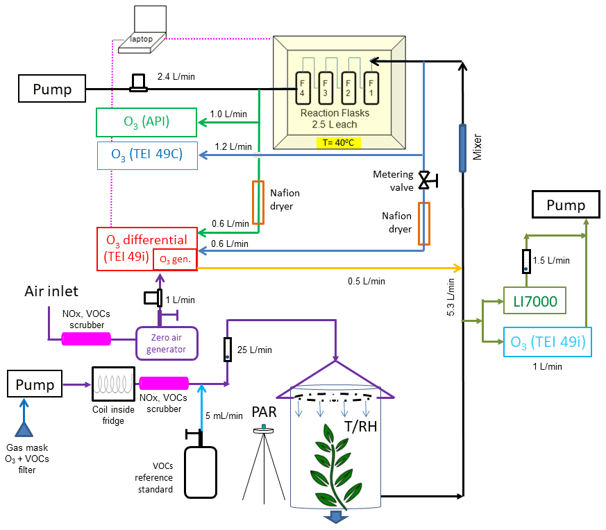
Figure 5Total ozone reactivity monitor experiment as used in the field study (results shown in Fig. 6) with the differential ozone monitor, the sampling line pressure balancing valve, and the Nafion dryers. Note that this schematic does not include the purge flows for the Nafion dryers. These are described in Fig. 3b. Additional instrumentation for the monitoring of O3 (TEI 419i), H2O, and CO2 (LI7000) in the air drawn from enclosure is shown on the right.
3.2 Balancing of the ozone monitor inlet pressures
The readings from the differential ozone monitor are sensitive to the difference in the pressure in the two sampling lines that connect upstream and downstream of the reactor (Supplement Sect. E). The pressure differential results from the vacuum generated by the sampling pump for providing flow through the reactor. The 49i diagnostics menu allows monitoring of the pressures of the two optical cells. In the original configuration, it was found that there was a pressure difference of, depending of the flow rate, i.e., 20–30 torr between the two cells at a 4 L min−1 reactor flow, with the lower pressure recorded in the line downstream of the reactor. This pressure differential alternates between negative and positive values as the monitor alternates air from the two inlets through the two optical cells. This pressure difference results in an artificial ozone signal offset between the two sampling paths. An increase in the flow rate through the reactor causes a change in the pressure difference and the ozone differential reported by the monitor: increasing the flow rate from 2 to 9 L min−1 corresponded to an increase from 2 to 7 ppb in the differential ozone signal. This behavior is clearly a measurement artifact and counter to the expected ozone loss, as the actual chemical ozone loss decreases with decreasing residence time of the air inside the reactor (i.e., increasing flow rate). This measurement artifact was mitigated by inserting a 0.64 cm Teflon metering valve into the ozone monitor sampling line that pulled air from upstream of the reactor (Fig. 3a). By closing the valve slightly, the flow was restricted to where both cell pressure readings from the reactor were equal (within ≈ 1 torr). This resulted in an ozone differential signal of ≈ 1.7 ppb that was insensitive to the reactor flow rate (Supplement Sect. E). The integration of the TORM into a vegetation enclosure experiment is shown in Fig. 5.
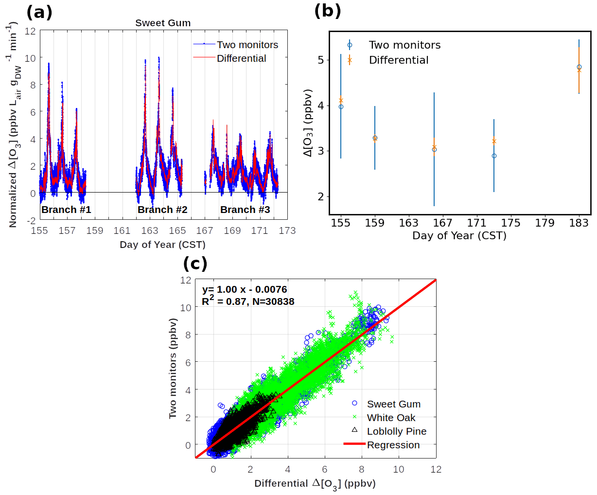
Figure 6Results from comparisons of monitoring the ozone loss in the reactor with two monitors versus measuring the ozone differential directly with the configuration shown in Fig. 5. (a) Three multi-day experiments of Δ[O3] monitoring from an enclosure of sweetgum branches. Data are also corrected for the empty bag OWL data shown in panel (b) and normalized for flow through the enclosure and dried weight of leaf biomass. (b) Δ[O3] determinations from blank experiments on an empty enclosure. (c) Summary results of experiments on a total of three different vegetation species. All field experiment results are from the Southern Oxidant and Aerosol Study (SOAS) campaign between June and July 2013 at a field site in Perry County, western central Alabama (Praplan et al., 2022).
3.3 Evaluation of the direct differential ozone reactivity measurement
Results from the parallel operation of two ozone monitors measuring the actual ozone before and after the reactor, with Δ[O3] calculated from the difference of the two readings, compared to the direct ozone differential measurement by TORM are summarized in Fig. 6. Field data, collected during the Southern Oxidant and Aerosol Study (SOAS) (CU Boulder system), constitute a total of 10 d of measurements collected using branch enclosures on three different branches of sweetgum trees. The OWL to the TORM was determined on five occasions by sampling from an empty bag. In these field conditions, the background differential signal (3–5 ppb, Fig. 6b) was somewhat higher than in the laboratory experiments described in the previous section. The OWL results bracketing the vegetation enclosure experiments were averaged and subtracted from the recordings of the enclosure experiments in between. The ozone differential was normalized to the airflow through the chamber and to the dried weight of leaf biomass that was sampled from the vegetation in the branch enclosure. These time series data show a clear diurnal cycle with the ozone differential increasing steeply during daytime hours. Results are reasonably consistent between days and the three different enclosures, considering that the BVOC emissions that determine this signal are highly sensitive to light and the enclosure temperature, which varied during the experiment. There is high agreement between the Δ[O3] results from both configurations across these experiments. A linear regression between results from the two monitoring methods from the SOAS yields a slope value of 0.996. The graphed data also show the substantial improvement in the noise of the measurement with the direct differential monitoring (Fig. 6a and b). After the system equilibration, the 1σ standard deviation of the differential ozone measurement for 1 min averaged readings was generally in the range of 0.1–0.2 ppb, which was 2–3 times lower than the calculated ozone difference from the two-monitor measurement. These results clearly indicate the benefits of the single-monitor measurement: (1) the accuracy of the differential signal is consistent with the differential two-monitor determination, (2) there is a significant improvement in the measurement precision from using a single monitor, and (3) the operation of a single monitor is less tedious and labor-intensive as it does not require regular intercomparison for determination of offsets and drifts or correction algorithms for calibrating the response of two individual monitors (Bocquet et al., 2011; Sommariva et al., 2020).
3.4 Sample residence time in the reactor
The desired operation of a flow reactor system is for air to move through the reactor as a narrow plug, with minimal turbulence and mixing. Most flow reactors are tubular and linear and are used in laboratory settings. Depending on their operational variables, they achieve seconds to a few minutes of residence time. The residence time and peak broadening during transport through the reactor were studied by installing a syringe injection port upstream of the reactor, injection of a small volume of a 1 ppm standard of nitric oxide (NO), and monitoring the ozone loss from the ozone + NO reaction downstream of the reactor with a fast-response (5 Hz) nitric oxide chemiluminescence instrument. Experiments were conducted in two different configurations: (1) in the normal plumbing configuration, with the incoming air introduced to each flask through the dip tube. (2) To test the effect of the dip tube, the plumbing was also reversed. The flow through the reactor was set to 4 L min−1, which for an ideal flow reactor at 10 L volume should result in a 150 s residence time. Results of these tests are shown in Fig. 7. For both configurations, the peak signal was observed earlier than the theoretical time, i.e., ≈ 18 s earlier for the normal configuration and ≈ 50 s earlier for the reversed configuration. The peak widths (at half of peak maximum) were ≈ 90 and 120 s for the normal and reversed configuration, respectively. The behavior in these data shows that there is a considerable amount of mixing inside the reactor glass flasks, causing deviation from an ideal flow reactor. Nonetheless, the residence time of ≈ 120 s for the normal plumbing configuration is sufficient to allow ozone to react with the sample so that a large enough differential signal can be measured. The findings from this experiment were confirmed at a higher 6 L min−1 flow rate (Supplement Sect. F). Both experiments show the advantage of the air introduction through the dip tube, resulting in a narrower peak, i.e., narrower defined residence time. For this configuration of the reactor, the mean residence time is about 90 % of the theoretical residence time.
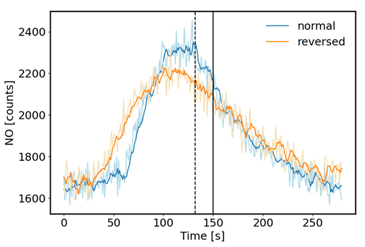
Figure 7Test of sample air residence time in the flow reactor. A small volume of a 1 ppm NO standard was injected through a port upstream of the reactor, and NO was monitored downstream with a fast-response chemiluminescence analyzer (1 s time resolution). 5 s running averages are presented here. The normal configuration was with the flow entering each flask through the dip tube. The reversed configuration was with the airflow exiting each flask through the dip tube. The vertical black line indicates the theoretical residence time (150 s) based on the total flow rate (4 L min−1) and total volume (10 L) of the reactor, assuming that there was no mixing inside the flasks. The dotted line depicts the mean of the distribution at 132 s for the normal configuration.
3.5 Evaluation and mitigation of humidity effects
As elucidated on in the Introduction, changes in humidity can severely interfere with the ozone determination (Wilson and Birks, 2006; Spicer et al., 2010). Ozone monitors have been found to be less sensitive, i.e., to report ozone below its actual value at high humidity, and to exhibit large artificial signal fluctuations from rapid changes in the sample water vapor. Characterization and mediation of the sensitivity of the ozone reactivity measurement to water vapor were a main emphasis of our experiments. Earlier experiments, wherein the sampling flow was subjected to variable water vapor, such as by injecting small volumes of water through an injection port upstream of the reactor in the configuration shown in Supplement Sect. C, confirmed the findings from prior literature: despite a constant ozone mole fraction that was fed into the reactor, both the two-monitor determination and the single monitor ozone differential determination showed instantaneous changes in the ozone signal, reaching on the order of 10 ppb. This bias in the ozone recording lasted significantly longer (≈ 10 times) than the residence time that was determined in the above-described experiment using nitric oxide, demonstrating that the retention of water, likely from reversible uptake to walls and tubing inner surfaces in the reactor, is longer, and flushing water vapor out of the reactor takes a higher purge volume than for less polar and/or more volatile gases. These water vapor effects on the ozone signal were mitigated by two modifications to the TORM. (1) The glass flask reactor was insulated, and a heater, regulated by a temperature controller, was added to control the temperature of the reactor to 40 ∘C. This heating significantly reduced the residence and interference time from the water injection, likely due to a reduction of the adherence of the water vapor to the walls of the glass flasks and other reactor components. Our observations agree with the findings reported by Wilson and Birks (2006), who found a reduction of the water interference for their 2B Technologies ozone monitor when the glass optical cell was slightly heated. (2) Nafion dryers (0.64 cm o.d. × 180 cm length; MD-110-72739 gas dryer, Perma Pure LLC, New Jersey, USA) were inserted into both ozone monitor inlet flows (sampling air before and after the reactor). We installed the two Nafion dryers there, rather than one Nafion dryer for the sample flow path going into the reactor, to prevent possible losses of polar and unsaturated compounds from the sample flow passing through a Nafion dryer, as has been reported in other prior research. The purge flow for the Nafion dryers was provided by the vent flow from the TEI 49i. The analyzer vent flow was split into two approximately equal fractions, resulting in 0.6 L min−1 flow for each Nafion dryer (Fig. 3b). Throttle valves were installed in both lines as flow restrictors and adjusted such that the pressure in the exterior chamber of the Nafion dryers was ≈ 10 % below the interior section of the dryer (cell pressure readings from the differential 49i monitor). The Nafion dryers were conditioned using the same protocol as for the reactor (see above), after which there was no notable ozone loss from sampling the ozone-enriched airflow through the Nafion tubing, in agreement with other previous studies that have reported negligible ozone loss in ozone-conditioned Nafion tubing materials (Wilson and Birks, 2006; Boylan et al., 2014; Kim et al., 2020).
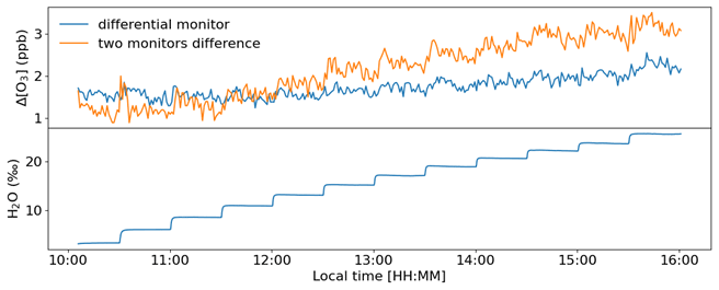
Figure 8Experiment with increasing humidity in the air supplied to the TORM. The humidity content of the sample air is displayed in the lower graph in units of parts per thousand (‰). A total of 12 levels were administered from ≈ 3 ‰–26 ‰, which at room temperature conditions (25 ∘C) is approximately equivalent to an RH range of 10 %–84 %.
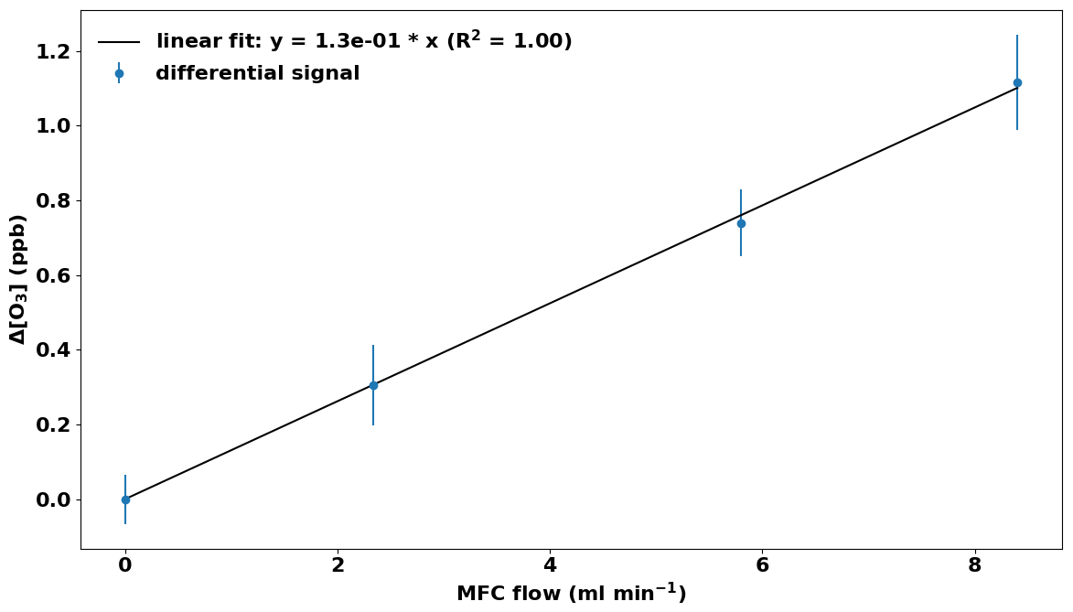
Figure 9Laboratory test of the TORM. A small flow of a high-mole-fraction limonene standard was fed into the system upstream of the reactor. Error bars represent the standard deviation for the monitoring data at each level.
Results from an experiment with the Nafion dryers in use and where water vapor was increased in multiple steps are shown in Fig. 8. The same humidification system as described by Boylan et al. (2014) was used to moisturize a zero air dilution gas fed to the TORM. The resulting humidity was recorded with a LI-COR model 7000 CO2–H2O gas analyzer downstream of the mixer, but upstream of the reactor. Each humidity level was maintained for 30 min before subjecting the system to the next higher moisture level by a rapid change in the humidity generator set point. The differential signal was monitored with the differential 49i monitor, as well as by recording the absolute ozone upstream and downstream of the reactor with two individual monitors. Both ozone monitoring systems sampled through the Nafion tubing. Results of the experiment (Fig. 8) show a residual differential signal response of ≈ 0.5 ppb over an approximately 10 % to 84 % RH span for the differential monitor. The two-monitor Δ[O3] response is approximately 6 times as large. The spikes during the moisture transition periods seen in earlier experiments disappeared completely for the differential monitor. If background measurements are performed at a different RH than the ozone reactivity measurements, this residual differential signal needs to be taken into account on a case-by-case basis.
Similar order of magnitude results were obtained in a series of experiments wherein liquid water (20 to 100 µL) was injected into the sampling flow through a septum port upstream of the reactor. The Nafion dryer removed ≈ of the water interference, and the differential monitor response to the water injection was approximately half compared to the calculated difference from the two-monitor configuration (Supplement Sect. G).
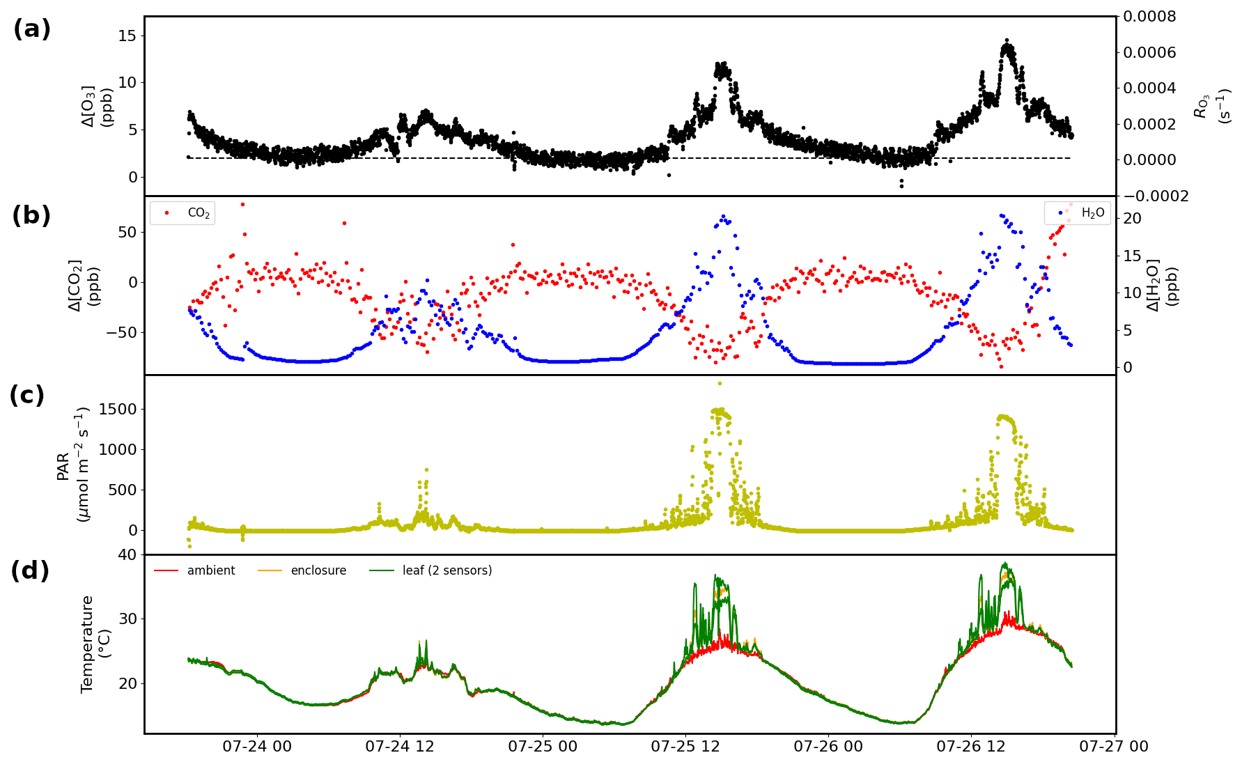
Figure 10Results obtained over 3 d from a branch enclosure experiment on a red oak tree at the University of Michigan Biological Station: (a) results for the Δ[O3] measurement, with the dashed black line indicating the value of the wall losses and/or background (left) and the corresponding RO3 (right). (b) Respiration and photosynthesis expressed as the difference in the water (right) and CO2 (left) mole fractions in the airstream going into and out of the enclosure. (c) Solar photosynthetically active radiation (PAR). (d) Leaf, inside enclosure, and ambient temperature.
3.6 Application examples
Ozone reactivity values of test mixtures and samples from vegetation enclosures were investigated. Results from a laboratory experiment using a flow of limonene test gas are presented in Fig. 9. The purpose of the experiment was to demonstrate the linearity of the TORM. The test gas was prepared in-house for a target mole fraction of 20 ppm, but the actual mole fraction could not be independently verified at the time of the experiment. The TORM determination shows good linearity, with an R2 result of the linear regression of 1.00. At the highest limonene level, the TORM signal recorded with the differential ozone monitor was 1.1 ppb (after subtraction of the 1.7 ppb Δ[O3] OWL that was determined for this particular application), which corresponds to a total O3 reactivity of 7.3 e−5 s−1, considering [O3]0 to be 100 ppb and the residence time 150 s (3.6 L min−1 flow through the 10 L reactor, scaled with a factor of 0.9). This indicates that the limonene mixing ratio entering the reactor was 13.6 ppb, which is reasonable considering the dilution from the gas standard (8.4 mL min−1 standard flow in a 5.1 L min−1 total flow) and its target mole fraction.
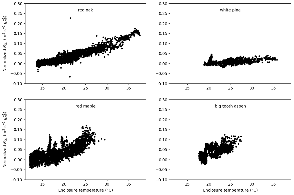
Figure 11Total O3 reactivity from the emissions results from experiments on red oak, red maple, white pine, and big tooth aspen at the University of Michigan Biological Station normalized to the amount of leaf dry mass and flow rate as a function of enclosure temperature.
The TORM has been deployed in field settings at several research sites in the USA and in Finland. Figure 10 displays more results from one of these field experiments, i.e., a 3 d branch enclosure experiment on a red oak tree at the University of Michigan Biological Station (UMBS) in 2010. The experiment was conducted on relatively warm and sunny days as can be seen in the radiation and temperature data. Besides the differential signal and the calculated total ozone reactivity, both shown in Fig. 10a (differential signal scale on the left and total ozone reactivity scale on the right), there were concurrent measurements of respiration, photosynthesis, photochemical active radiation (PAR), and ambient, leaf, and enclosure temperature. The change in humidity, reaching a maximum of the order of 25 ‰ as the midday maximum when foliage respiration peaks, confirms our estimate presented in the Introduction for the humidity changes during vegetation enclosure experiments. Emission samples collected from this enclosure and analyzed by gas chromatography showed that emissions from this branch were dominated by isoprene, with further substantial emissions of MT and SQT compounds. On both days, the TORM recorded a midday maximum differential ozone signal of 12–14 ppb, dropping to 2–3 ppb at night, which is close to the system background signal (OWL). The differential signal clearly follows a daily cycle, with low values during nighttime hours and daytime maxima during the early afternoon. The ozone reactivity signal maxima coincide with the peak in diurnal radiation, respiration, and photosynthesis, which suggests that the ozone-reactive emissions are modulated by light availability. Similar diurnal cycles of ozone reactivity were observed for sweetgum in the Southern Oxidant and Aerosol Study (Park et al., 2013), as can be seen in the 10 d of measurements shown in Fig. 6. Please note that the data in Fig. 6 were normalized to the leaf dry mass of the enclosure foliage. A detailed discussion comparing the observed total ozone reactivity with the ozone reactivity calculated from identified BVOC species in the emissions is the subject of an upcoming publication (Praplan et al., 2022).
Furthermore, a presentation of the ozone reactivity results normalized to the leaf dry mass and flow through the branch chamber as a function of leaf temperature for experiments performed at UMBS is shown in Fig. 11. All four species show an increase in reactivity with increasing temperature. This feature indicates that all species emit reactive volatiles at increasing rates as temperature increases. Interestingly, the normalized reactivity for the various tree species is quite different, varying by at least a factor of 3. It also appears that the temperature dependencies are different, with red maple showing a more dynamic increase than other species. Remarkably, white pine, a high MT emitter, gave the lowest reactivity results. Furthermore, the ozone reactivity temperature response for red maple appears to be higher than for red oak, despite the fact that red oak was found to emit higher amounts of BVOCs than maple, but with most of the emissions made up by isoprene. The relatively high levels of ozone reactivity are also noteworthy in light of the independent OH reactivity study by Kim et al. (2011), who found that red maple emissions exhibited the highest missing OH reactivity associated with SQT in comparison with these other three species. Consequently, red maple is a prime candidate for having reactive BVOC emissions that hitherto have not been chemically identified.
A total ozone reactivity monitor, TORM, was developed for the study of the ozone reactivity of biogenic emissions. TORM builds on standard laboratory equipment and can be assembled with moderately technically skilled personnel at a relatively moderate cost. The instrument was thoroughly characterized, and a number of ameliorations were implemented that significantly improved the measurement sensitivity and reduced the interference from absolute and changing water vapor in the sample air. Critical improvements over previously reported measurement approaches were the adaptation of a commercial ozone UV absorption monitor for direct measurement of the reacted ozone (ozone differential), heating and temperature control of the reactor, and the drying of the sample flows with Nafion dryers. Specific challenges arose with this setup that could be overcome, such as balancing the pressure difference for each cell in the differential ozone monitor (one cell measuring ozone in air sampled before the reactor and the other cell measuring after).
TORM has been used in a number of field settings and proven the feasibility and value of this new measurement. Differential ozone signals (Δ[O3]) on the order of 0–10 ppb have been obtained in enclosure experiments with high-BVOC-emitting species. These signals are 20–50 times above the noise level of the measurement. Chemical identification of BVOC emissions from the enclosure and estimation of the total reactivity of identified emissions have been able to only account for a fraction of the directly measured ozone reactivity. A detailed description of these field studies and discussion of the results, including the attribution of the directly measured ozone reactivity to identified BVOC emissions, will be presented in a forthcoming publication (Praplan et al., 2022).
All data that the work builds on are presented in the paper and the Supplement.
The supplement related to this article is available online at: https://doi.org/10.5194/amt-15-5439-2022-supplement.
DH was the principal investigator of the US study. DH advised student researchers, managed research grants, oversaw the study, and prepared and approved the paper. AG was the co-principal investigator of the US study. AG reviewed and approved the paper. JH constructed instrumentation and conducted experiments, developed control and data acquisition software, and approved the paper. RD constructed instrumentation and conducted experiments, participated in field studies, and reviewed and approved the paper. WW constructed instrumentation, conducted experiments, and prepared, reviewed, and approved the paper. JHP constructed instrumentation, developed instrument control software, conducted lab and field experiments, and reviewed and approved the paper. AL constructed instrumentation, conducted lab and field experiments, and approved the paper. APP was the principal investigator of the Finnish study. APP conducted field as well as lab experiments and prepared and approved the paper.
The contact author has declared that none of the authors has any competing interests.
This study does not necessarily reflect the views of the funding agencies, and no official endorsements should be inferred.
Publisher's note: Copernicus Publications remains neutral with regard to jurisdictional claims in published maps and institutional affiliations.
The development and testing of the TORM system has been made possible through funding from the US National Science Foundation under grants AGS 0904139, ATM-1140571, and AGS-1561755, as well as funding from the Academy of Finland (decisions nos. 307797 and 314099).
This paper was edited by Anna Novelli and reviewed by two anonymous referees.
Altimir, N., Tuovinen, J. P., Vesala, T., Kulmala, M., and Hari, P.: Measurements of ozone removal by Scots pine shoots: calibration of a stomatal uptake model including the non-stomatal component, Atmos. Environ., 38, 2387–2398, https://doi.org/10.1016/j.atmosenv.2003.09.077, 2004.
Altimir, N., Kolari, P., Tuovinen, J.-P., Vesala, T., Bäck, J., Suni, T., Kulmala, M., and Hari, P.: Foliage surface ozone deposition: a role for surface moisture?, Biogeosciences, 3, 209–228, https://doi.org/10.5194/bg-3-209-2006, 2006.
Bocquet, F., Helmig, D., Van Dam, B. A., and Fairall, C. W.: Evaluation of the flux gradient technique for measurement of ozone surface fluxes over snowpack at Summit, Greenland, Atmos. Meas. Tech., 4, 2305–2321, https://doi.org/10.5194/amt-4-2305-2011, 2011.
Bouvier-Brown, N. C., Goldstein, A. H., Worton, D. R., Matross, D. M., Gilman, J. B., Kuster, W. C., Welsh-Bon, D., Warneke, C., de Gouw, J. A., Cahill, T. M., and Holzinger, R.: Methyl chavicol: characterization of its biogenic emission rate, abundance, and oxidation products in the atmosphere, Atmos. Chem. Phys., 9, 2061–2074, https://doi.org/10.5194/acp-9-2061-2009, 2009a.
Bouvier-Brown, N. C., Holzinger, R., Palitzsch, K., and Goldstein, A. H.: Large emissions of sesquiterpenes and methyl chavicol quantified from branch enclosure measurements, Atmos. Environ., 43, 389–401, https://doi.org/10.1016/j.atmosenv.2008.08.039, 2009b.
Boylan, P., Helmig, D., and Park, J.-H.: Characterization and mitigation of water vapor effects in the measurement of ozone by chemiluminescence with nitric oxide, Atmos. Meas. Tech., 7, 1231–1244, https://doi.org/10.5194/amt-7-1231-2014, 2014.
Di Carlo, P., Brune, W. H., Martinez, M., Harder, H., Lesher, R., Ren, X. R., Thornberry, T., Carroll, M. A., Young, V., Shepson, P. B., Riemer, D., Apel, E., and Campbell, C.: Missing OH reactivity in a forest: Evidence for unknown reactive biogenic VOCs, Science, 304, 722–725, 2004.
Duhl, T. R., Helmig, D., and Guenther, A.: Sesquiterpene emissions from vegetation: a review, Biogeosciences, 5, 761–777, https://doi.org/10.5194/bg-5-761-2008, 2008.
Fares, S., Goldstein, A., and Loreto, F.: Determinants of ozone fluxes and metrics for ozone risk assessment in plants, J. Exp. Bot., 61, 629–633, https://doi.org/10.1093/jxb/erp336, 2010a.
Fares, S., McKay, M., Holzinger, R., and Goldstein, A. H.: Ozone fluxes in a Pinus ponderosa ecosystem are dominated by non-stomatal processes: Evidence from long-term continuous measurements, Agr. Forest Meteorol., 150, 420–431, 2010b.
Fares, S., Park, J. H., Ormeno, E., Gentner, D. R., McKay, M., Loreto, F., Karlik, J., and Goldstein, A. H.: Ozone uptake by citrus trees exposed to a range of ozone concentrations, Atmos. Environ., 44, 3404–3412, https://doi.org/10.1016/j.atmosenv.2010.06.010, 2010c.
Goldstein, A. H., McKay, M., Kurpius, M. R., Schade, G. W., Lee, A., Holzinger, R., and Rasmussen, R. A.: Forest thinning experiment confirms ozone deposition to forest canopy is dominated by reaction with biogenic VOCs, Geophys. Res. Lett., 31, L22106, https://doi.org/10.1029/2004gl021259, 2004.
Helmig, D., Daly, R., and Bertman, S. B.: Ozone reactivity of biogenic volatile organic compounds from four dominant tree species at PROPHET-CABINEX, 2010 Fall Meeting, AGU, San Francisco, Calif., 13–17 December 2010, Abstract A53C-0240, 2010.
Hogg, A., Uddling, J., Ellsworth, D., Carroll, M. A., Pressley, S., Lamb, B., and Vogel, C.: Stomatal and non-stomatal fluxes of ozone to a northern mixed hardwood forest, Tellus B, 59, 514–525, https://doi.org/10.1111/j.1600-0889.2007.00269.x, 2007.
Holzinger, R., Lee, A., Paw, K. T., and Goldstein, U. A. H.: Observations of oxidation products above a forest imply biogenic emissions of very reactive compounds, Atmos. Chem. Phys., 5, 67–75, https://doi.org/10.5194/acp-5-67-2005, 2005.
Kim, D. J., Dinh, T. V., Lee, J. Y., Choi, I. Y., Son, D. J., Kim, I. Y., Sunwoo, Y., and Kim, J. C.: Effects of water removal devices on ambient inorganic air pollutant measurements, Int. J. Env. Res. Public He., 16, 1–9, https://doi.org/10.3390/ijerph16183446, 2019.
Kim, D. J., Dinh, T. V., Lee, J. Y., Son, D. J., and Kim, J. C.: Effect of nafion dryer and cooler on ambient air pollutant (O3, SO2, CO) Measurement, Asian J. Atmos. Environ., 14, 28–34, https://doi.org/10.5572/ajae.2020.14.1.028, 2020.
Kim, S., Guenther, A., Karl, T., and Greenberg, J.: Contributions of primary and secondary biogenic VOC tototal OH reactivity during the CABINEX (Community Atmosphere-Biosphere INteractions Experiments)-09 field campaign, Atmos. Chem. Phys., 11, 8613–8623, https://doi.org/10.5194/acp-11-8613-2011, 2011.
Kurpius, M. R., and Goldstein, A. H.: Gas-phase chemistry dominates O3 loss to a forest, implying a source of aerosols and hydroxyl radicals to the atmosphere, Geophys. Res. Lett., 30, https://doi.org/10.1029/2002gl016785, 2003.
Lenschow, D. H., Pearson, R., and Stankov, B. B.: Estimating the ozone budget in the boundary-layer by use of aircraft measurements of ozoneeddy flux and mean concentration, J. Geophys. Res.-Oceans, 86, 7291–7297, https://doi.org/10.1029/JC086iC08p07291, 1981.
Lenschow, D. H., Pearson, R., and Stankov, B. B.: Measurements of ozone vertical flux to ocean and forest, J. Geophys. Res.-Oceans, 87, 8833–8837, https://doi.org/10.1029/JC087iC11p08833, 1982.
Lou, S., Holland, F., Rohrer, F., Lu, K., Bohn, B., Brauers, T., Chang, C. C., Fuchs, H., Häseler, R., Kita, K., Kondo, Y., Li, X., Shao, M., Zeng, L., Wahner, A., Zhang, Y., Wang, W., and Hofzumahaus, A.: Atmospheric OH reactivities in the Pearl River Delta – China in summer 2006: measurement and model results, Atmos. Chem. Phys., 10, 11243–11260, https://doi.org/10.5194/acp-10-11243-2010, 2010.
Matsumoto, J.: Measuring Biogenic Volatile Organic Compounds (BVOCs) from Vegetation in Terms of Ozone Reactivity, Aerosol Air Qual. Res., 14, 197–206, https://doi.org/10.4209/aaqr.2012.10.0275, 2014.
Matthews, R. D., Sawyer, R. F., and Schefer, R. W.: Interferences in chemiluminescence measurement of NO and NO2 emissions from combustion systems, Environ. Sci. Technol., 11, 1092–1096, 1977.
McKinney, K. A., Lee, B. H., Vasta, A., Pho, T. V., and Munger, J. W.: Emissions of isoprenoids and oxygenated biogenic volatile organic compounds from a New England mixed forest, Atmos. Chem. Phys., 11, 4807–4831, https://doi.org/10.5194/acp-11-4807-2011, 2011.
Misztal, P. K., Owen, S. M., Guenther, A. B., Rasmussen, R., Geron, C., Harley, P., Phillips, G. J., Ryan, A., Edwards, D. P., Hewitt, C. N., Nemitz, E., Siong, J., Heal, M. R., and Cape, J. N.: Large estragole fluxes from oil palms in Borneo, Atmos. Chem. Phys., 10, 4343–4358, https://doi.org/10.5194/acp-10-4343-2010, 2010.
Ortega, J. and Helmig, D.: Approaches for quantifying reactive and low-volatility biogenic organic compound emissions by vegetation enclosure techniques – Part A, Chemosphere, 72, 343–364, https://doi.org/10.1016/j.chemosphere.2007.11.020, 2008.
Ortega, J., Helmig, D., Guenther, A., Harley, P., Pressley, S., and Vogel, C.: Flux estimates and OH reaction potential of reactive biogenic volatile organic compounds (BVOCs) from a mixed northern hardwood forest, Atmos. Environ., 41, 5479–5495, https://doi.org/10.1016/j.atmosenv.2006.12.033, 2007.
Ortega, J., Helmig, D., Daly, R. W., Tanner, D. M., Guenther, A. B., and Herrick, J. D.: Approaches for quantifying reactive and low-volatility biogenic organic compound emissions by vegetation enclosure techniques – Part B: Applications, Chemosphere, 72, 365–380, https://doi.org/10.1016/j.chemosphere.2008.02.054, 2008.
Park, J., Guenther, A. B., and Helmig, D.: Ozone reactivity of biogenic volatile organic compound (BVOC) emissions during the Southeast Oxidant and Aerosol Study (SOAS), in: American Geophysical Union, Fall Meeting 2013 , abstract #A13A-0172, https://ui.adsabs.harvard.edu/abs/2013AGUFM.A13A0172P/abstract (last access: 5 August 2022), 2013.
Praplan, A. P., Daly, R. W., Park, J.-H., Liikanen, A., Angot, H., Huber, J., Bertman, S. B., Guenther, A., and Helmig, D.: Applications for the total ozone reactivity monitor (TORM), in preparation, 2022.
Ridley, B. A., Grahek, F. E., and Walega, J. G.: A small, high-sensitivity, medium-response ozone detector suitable for measurements from light aircraft, J. Atmos. Ocean. Tech., 9, 142–148, https://doi.org/10.1175/1520-0426(1992)009<0142:ashsmr>2.0.co;2, 1992.
Sommariva, R., Kramer, L. J., Crilley, L. R., Alam, M. S., and Bloss, W. J.: An instrument for in situ measurement of total ozone reactivity, Atmos. Meas. Tech., 13, 1655–1670, https://doi.org/10.5194/amt-13-1655-2020, 2020.
Spicer, C. W., Joseph, D. W., and Ollison, W. M.: A Re-Examination of Ambient Air Ozone Monitor Interferences, J. Air Waste Manage., 60, 1353–1364, https://doi.org/10.3155/1047-3289.60.11.1353, 2010.
Wilson, K. L. and Birks, J. W.: Mechanism and elimination of a water vapor interference in the measurement of ozone by UV absorbance, Environ. Sci. Technol., 40, 6361–6367, https://doi.org/10.1021/es052590c, 2006.
Wolfe, G. M., Thornton, J. A., McKay, M., and Goldstein, A. H.: Forest-atmosphere exchange of ozone: sensitivity to very reactive biogenic VOC emissions and implications for in-canopy photochemistry, Atmos. Chem. Phys., 11, 7875–7891, https://doi.org/10.5194/acp-11-7875-2011, 2011.