the Creative Commons Attribution 4.0 License.
the Creative Commons Attribution 4.0 License.
 | 27 Sep 2022
Towards vertical wind and turbulent flux estimation with multicopter uncrewed aircraft systems
Tamino Wetz
Vertical wind velocity and its fluctuations are essential parameters in the atmospheric boundary layer (ABL) to determine turbulent fluxes and scaling parameters for ABL processes. The typical instrument to measure fluxes of momentum and heat in the surface layer are sonic anemometers. Without the infrastructure of meteorological masts and above the typical heights of these masts, in situ point measurements of the three-dimensional wind vector are hardly available. We present a method to obtain the three-dimensional wind vector from avionic data of small multicopter uncrewed aircraft systems (UAS). To achieve a good accuracy in both average and fluctuating parts of the wind components, calibrated motor thrusts and measured accelerations by the UAS are used. In a validation campaign, in comparison to sonic anemometers on a 99 m mast, accuracies below 0.2 m s−1 are achieved for the mean wind components and below 0.2 m2 s−2 for their variances. The spectra of variances and covariances show good agreement with the sonic anemometer up to 1 Hz temporal resolution. A case study of continuous measurements in a morning transition of a convective boundary layer with five UAS illustrates the potential of such measurements for ABL research.
- Article
(4461 KB) - Full-text XML
- BibTeX
- EndNote


The nature of turbulence in the atmospheric boundary layer (ABL) is multifaceted and depends on internal and external parameters such as thermal stratification and shear, surface heat fluxes, and surface roughness. Turbulent fluxes of momentum and heat are the main driver for mixing in the ABL and thus determine its diurnal cycle. Determining turbulent fluxes requires measuring the three-dimensional wind vector and temperature with a temporal resolution that covers all turbulent scales that contribute significantly to the process. The eddy covariance (EC) method is a way to determine the momentum fluxes from the covariances of the wind components , , and the heat flux from the covariance between potential temperature and vertical wind (Aubinet et al., 2012). From the fluxes, scaling parameters for the ABL such as shear stress u*, convective velocity scale w*, Obukhov length L, and Richardson number Ri can be derived (Stull, 1988), which are essential for a profound understanding of boundary layer processes. It is thus evident that the measurement of vertical wind velocity and its fluctuations is crucial.
In practice, the most prominent instrument to measure turbulent fluxes in the ABL is the three-dimensional sonic anemometer (Kaimal and Businger, 1963) which has undergone extensive development and commercialization since the 1990s and is nowadays the essential part of every surface energy balance station (Mauder and Zeeman, 2018). Operating sonic anemometers is mostly limited to the surface layer (Baldocchi et al., 2001) or requires meteorological masts to reach heights up to 300 m above ground, which involves significant costs and infrastructure (Wolfe and Lataitis, 2018). To obtain representative quantities for a certain area with single point measurements, assumptions of homogeneity and ergodicity need to be made. It has recently been shown that coherent structures such as secondary circulations can violate the ergodicity assumption and lead to errors in the EC method (Mauder et al., 2020; Morrison et al., 2022). Only few experiments exist where multiple sonic anemometers have been installed over a wide area and heights above the surface layer, due to the large logistical effort. Some examples are the Great Belt Coherence experiment over water (Mann et al., 1991) and the Perdigão 2017 experiment in complex terrain (Fernando et al., 2019).
One possibility to obtain area-averaged fluxes are airborne measurements with research aircraft incorporating flow probes and fast temperature sensors. Such measurements can cover many square kilometers in a relatively short amount of time but also require assumptions of stationarity throughout the flight which can lead to sampling errors (Mahrt, 1998). To overcome limitations of crewed aircraft when flying at low altitudes and at lower costs, fixed-wing uncrewed aircraft systems (UAS) have been deployed in the past to measure turbulent fluxes (van den Kroonenberg et al., 2008; Wildmann et al., 2015).
To combine the benefits of the flexible deployment of UAS and allow point measurements instead of area-averaged measurements, multicopter UAS are a possible solution. Wetz et al. (2021) showed that such systems can be deployed in small fleets and obtain distributed horizontal wind measurements with a good accuracy. They become increasingly popular for vertical profiling of the ABL when temperature and humidity sensors are carried (Koch et al., 2018; Segales et al., 2020). The measurement of vertical velocity with such systems is, however, challenging due to the obvious distortion of the flow by the thrust of the rotors. Thielicke et al. (2021) showed that with a sonic anemometer installed on a multicopter in sufficient distance to the rotors, measurements of vertical wind are feasible. However, such a design increases the complexity of the flight system, its weight, and its cost. In order to operate a fleet of small and lightweight multicopter UAS, we propose a method to obtain the three-dimensional wind vector with avionic data alone, including calibrated motor thrust measurement. This is the first method that allows vertical wind and turbulent flux measurement with multicopter UAS without an external sensor.
In Sect. 2, we describe the UAS and the methodology to filter sensor data, calculate the forces that act on the UAS and calibrate the vertical velocity measurements. Section 3 describes the setting of the calibration and validation campaign at the boundary layer field site (Grenzschichtmessfeld, GM) Falkenberg of the German Meteorological Service (DWD). Section 4 contains the results of three-dimensional wind measurements, second-order statistics, and the derivation of momentum fluxes in comparison to measurements of sonic anemometers on a 99 m mast. A case study with measurements during a morning transition of a convective boundary layer illustrates the potential of the method. We conclude and give an outlook on future research in Sect. 5.
2.1 System description
We operate a fleet of 35 UAS of type Holybro QAV250 within the SWUF-3D project (Simultaneous Wind measurements with Unmanned Flight Systems in 3D). The main characteristics are described in Wetz et al. (2021). With a weight below 1 kg and a frame size of 0.25 m, the UAS are small enough to be operated in the open category of the European Regulation 2019/947. Operation in a fleet with fewer pilots than the UAS requires special permission from the flight authorities. A Pixhawk® 4 Mini autopilot is used as the flight controller and allows access to all avionic data, which are stored at high sampling rates on an internal SD card. The sampling rate depends on the type of data and is presented in more detail in Sect. 2.5. In the current configuration, flight times up to 17 min can be achieved. The UAS are operated in a weather vane mode, which means that a controller will minimize the roll angle so that the front side of the UAS will always face the wind in the main wind direction. Figure 1 shows two UAS in flight.
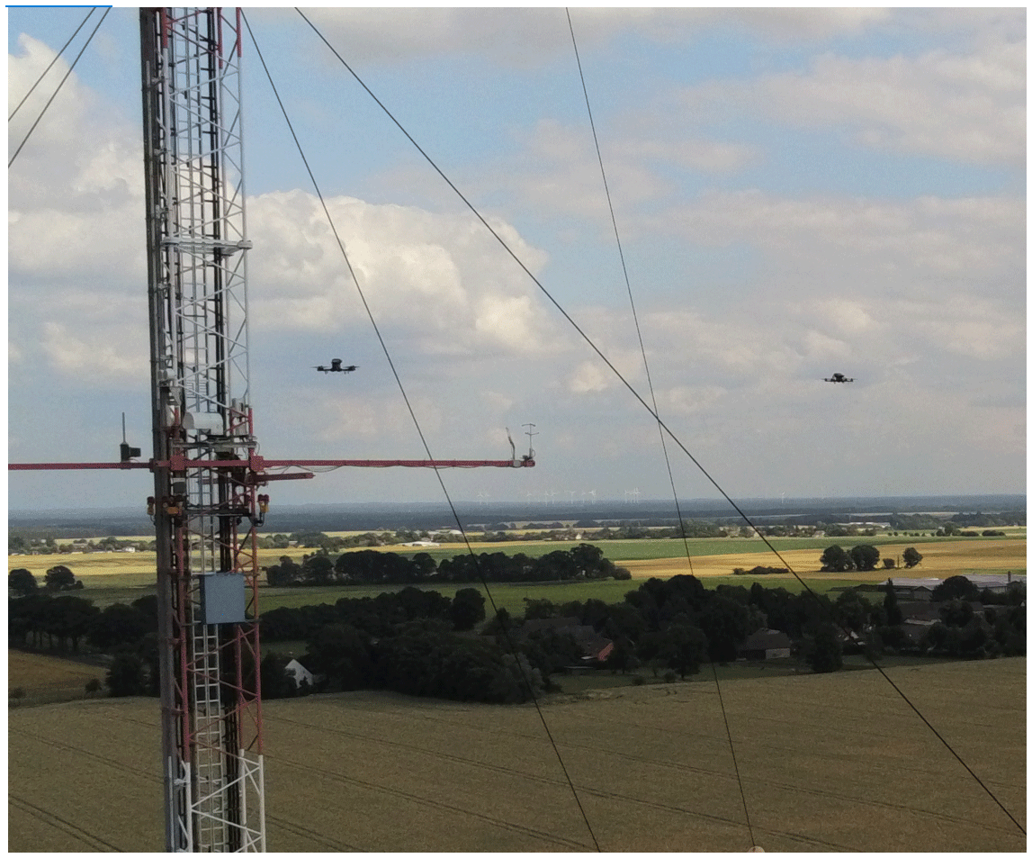
Figure 1Two Holybro QAV250 UAS in flight. In the background the 99 m mast with a sonic anemometer on the boom at 50 m can be seen.
2.2 Motor thrust calibration
In order to determine the forces that act on the UAS, it is important to know the actuator forces of the four rotors. There are no direct sensors for rotational speed, torque, or even thrust in the system. However, the motor controller PPM (pulse-position modulation) signal and the battery voltage and current are measured by the autopilot. The PPM signal is directly related to the voltage that is applied to the motor and is in theory directly proportional to the revolution speed. The voltage at each rotor is
with Ub the battery voltage and si the servo PPM command (smin for zero and smax for full throttle). It is important to include the battery voltage here as it decreases throughout the flight. Assuming a linear relationship for the electric servo motors, the revolution speed of each motor can be determined as
The motor thrust Ti can be calculated from the rotational speed Ωi, the rotor radius R, the rotor swept area A=πR2, air density ρ, and the thrust coefficient Ct (Leishman, 2016, Eq. 2.31):
In order to determine this relationship experimentally, in addition to the thrust coefficient of the rotor, which relates thrust to revolution speed, a hardware-in-the-loop test stand for a single motor–rotor setup is used. A schematic of the setup is shown in Fig. 2. We can thus determine the motor constant kV and the thrust coefficient Ct experimentally.
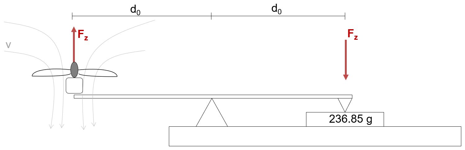
Figure 2Schematic of the motor test stand. The rotor is producing thrust in the free stream and the counteracting force of the equal length lever arm is measured with a scale on a table.
2.3 Quadrotor dynamics and rotor aerodynamics
To describe the motion of a quadrotor in three dimensions in its body-fixed frame of reference (x to the front, y to the right, z downwards), the rigid body model as described in Wetz et al. (2021) can be used. The force balance equations for translational motion within this model are as follows:
with m the mass of the UAS; p, q, and r the gyroscopic terms; g the acceleration due to gravity; and θ and φ the pitch and roll angle. The external forces are caused by wind. Equation (6) contains the total actuator thrust T, which counteracts all the external forces due to wind and gravity. The concept of operation for the UAS fleet is to hover at fixed positions so that motions due to maneuvering can be neglected. The variance of gyroscopic terms during hover periods is 2 orders of magnitude smaller than the variance of the acceleration terms. Gyroscopic terms of the force balance equation are thus neglected in the following. In Wetz et al. (2021), only the forces in the x direction in Eq. (4) were considered since the UAS yaws into the main wind direction, and the wind speed magnitude can thus be approximated by this one-dimensional simplification. In Wetz and Wildmann (2022), the two-dimensional wind vector was determined, including Eq. (5) in the algorithm and improving the dynamic response via the inclusion of the acceleration terms. In order to measure the full three-dimensional wind vector, Eq. (6) needs to be included. The single-motor thrusts Ti can be obtained from calibration as described in Sect. 2.2 and can be summed to obtain the total acting force . With increasing wind speed, the quadrotor lift not only generated rotor thrust, but aerodynamic effects will also start to occur. In theory, these effects are well described if the forward flight speed is much larger than the velocity that is induced by the rotor vi (V∞>>vi). Glauert's high-speed approximation (Leishman, 2016) gives an equation for the total resulting thrust for a single-rotor helicopter:
For the quadrotors used in this study, the induced velocity is on the order of 10 m s−1. This means that Glauert's approximation can not be used for hover flight and wind speeds of the same order of magnitude. Nevertheless, lift effects are observed by reduced power consumption and less required thrust in dependence of wind speed. We thus include a lift term FL in Eq. (6) to account for this effect but need to determine the relationship experimentally.
With the assumption of hover state and the additional term for aerodynamic lift, we can then solve Eqs. (4)–(6) for the external wind forces, so that
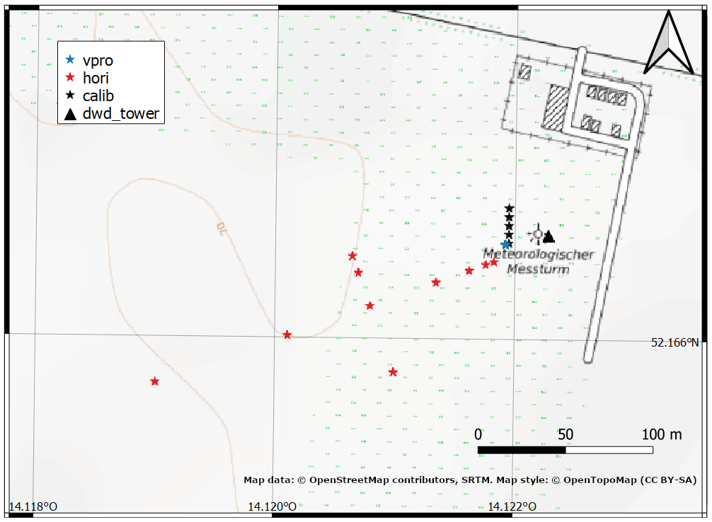
Figure 3Map of the GM Falkenberg site with the location of measurement points for the different flight patterns (stars) and the meteorological mast (black triangle). Background map data are taken from ©OpenStreetMap contributors, SRTM (map style: ©OpenTopoMap CC BY-SA).
2.4 Determination of the three-dimensional wind vector
To translate the forces that act on the quadrotor to wind speeds, a straightforward approach, as applied in Wetz et al. (2021), is the Rayleigh drag equation. It is, however, evident that the complex aerodynamic system of a multicopter is not perfectly represented by the physical relationships for solid bodies. Wetz and Wildmann (2022) have therefore allowed a calibration curve that is a power law with a free exponent. With this approach, higher accuracies are achievable. We apply this method here for all three dimensions, so that the wind components in the body frame of the quadrotor are
where the parameters b and c need to be calibrated for the respective direction. For the vertical direction, it is conceivable that upward and downward motion of the quadrotor relative to the air is subject to significantly different drag. For this reason, a distinction of cases is done for the z`component so that
The final step to obtain the meteorological wind vector is a rotation of the wind speeds from the body frame into the geodetic coordinates with the Euler angles of the quadrotor and a subtraction of the linear velocities (vx, vy, vz), which are measured by the autopilot on the basis of GNSS (global navigation satellite system) information:
2.5 Data preparation and filtering
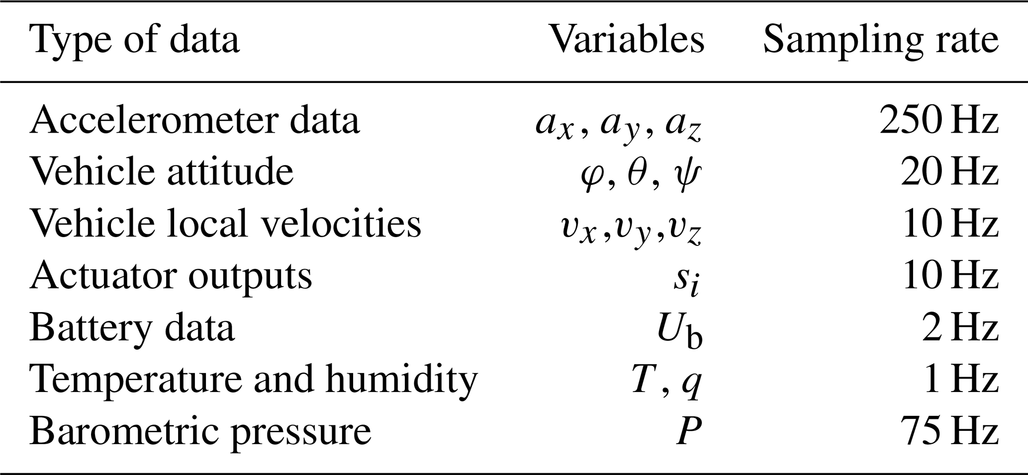
The raw sensor data of the UAS are stored on the SD card with different sampling rates depending on the data type but with a synchronized timestamp. Table 1 presents the raw data types and variables that are used for the wind calculation and their initial sampling rate. Reasons for the different sampling rates are the capabilities of the sensors and the requirements for the flight controller. Except for the battery data, all data are sampled with a rate of 10 Hz or higher. The raw data can be subject to significant noise in the high-frequency range due to sensor noise or vibrations. Preconditioning steps are taken before further processing of the data to obtain clean and synchronized data. Accelerometer data are filtered with a Butterworth filter to prevent anti-aliasing effects from frequencies above 10 Hz. All data are then interpolated and synchronized to a common time step with Δt=0.1 s. After this step, noise can still be recognized in accelerometer and actuator data, so that for the wind calculation, frequencies above 2 Hz are cut off with a fast Fourier transform (FFT) filter in the frequency domain.
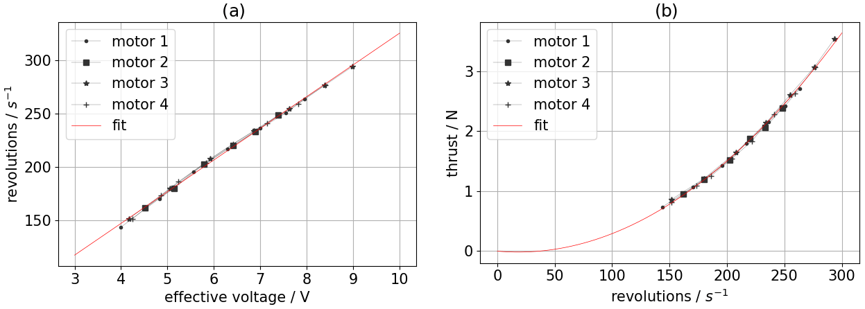
Figure 4Calibration results of the motor test stand. (a) The calibration curve of revolution speed versus applied voltage and (b) the thrust coefficient curve. The fitted calibration curves are shown as red lines.
2.6 Calculation of turbulence parameters
From the three-dimensional wind data, we can calculate momentum fluxes, friction velocity, and turbulence kinetic energy (TKE). Momentum fluxes are calculated as the covariances between the wind components, i.e., , , and . The friction velocity u* is calculated from the momentum fluxes according to Stull (1988):
TKE is defined as half of the sum of the variances of the three wind components:
A calibration and validation campaign for the SWUF-3D fleet was carried out in the framework of the FESSTVaL (Field Experiment on submesoscale spatiotemporal variability in Lindenberg) campaign in June/July 2021 at the GM Falkenberg site of the DWD. Figure 3 gives a map of the location with an indication of the measurement positions, including the location of the 99 m meteorological mast at the site. Two sonic anemometers (Metek UAS-1) are installed at 50 and 90 m height and serve as the reference for calibration and validation. Their measurements are distorted by the tower for wind directions between 345 and 50∘ via north and are thus disregarded for such conditions.
Calibration flights were done with five UAS at 50 and 90 m respectively, in close proximity (Δx=20 m) to the mast (see black stars in Fig. 3 and Wetz and Wildmann, 2022). During a morning transition of a convective boundary layer on 28 June 2021, continuous measurements were done with two sets of five UAS stacked in five heights (10, 50, 90, 150, 200 m) at the location of the blue star in Fig. 3. The two sets were measuring alternately in close separation of 5 m and with a short overlap of 1 min to guarantee continuous observations. Spatially distributed measurements (red stars) were performed to calculate coherence of the flow but are not analyzed in this study.
4.1 Motor test stand calibration
With Eq. (1), the voltage at the motor can be estimated from the actuator outputs. Results from the hardware-in-the-loop experiment (Fig. 4a) reveal a nearly linear relationship between voltage and revolution speed. The coefficient that relates voltage to revolution speed is .
From Fig. 4b we find that the thrust curve Ti as a function of revolution speed Ωi is best approximated with a polynomial of the second order. Such behavior is quite common and has been described before (Bangura et al., 2016). We determine the calibration curve as follows:
4.2 In-flight wind vector calibration
For calibration of the dynamic equations as described in Sect. 2.3, we use UAS#12 because it was operating in most of the calibration flights (i.e., 14 flights, with a wind speed range of 1–8 m s−1). The results of the calibration of the horizontal wind components are presented in Wetz and Wildmann (2022). In this study, we focus on the calibration of the vertical velocity component. This calibration is done in two steps. First, the lift force, which reduces the necessary thrust in hover flight, is determined as a function of the wind speed in the x direction. Second, thrust minus lift is calibrated against the vertical wind velocity as measured by the sonic anemometers at the 99 m mast.
4.2.1 Lift force
To estimate the lift force FL, we analyze the measured thrust force during all calibration flights in dependency of the horizontal wind. Horizontal wind is not known a priori, so we use the drag force in x-direction in the body frame Fx as a proxy which depends on the wind speed as described by Eqs. (8) and (11). It is not possible in a field experiment to perfectly decouple the lift effects from the wind in x-direction from the drag and lift in z-direction. For calibration purposes, we assume that the x and z-component of the wind are uncorrelated and that vertical wind is normally distributed around zero. To reduce the scatter, a 10 s moving average is applied to the data. Figure 5 shows the point cloud of lift versus drag force in x-direction for all calibration flights of UAS#12. The red line gives a polynomial fit. It can be seen that significant lift is generated up to Fx≈1 N lift, before it abruptly decreases, as it is typical for stall conditions. This force in x-direction corresponds to a horizontal wind speed of approximately 8 m s−1. Beyond that wind speed, only a few data are available, which yields a high uncertainty in the calibration at higher wind speed conditions.
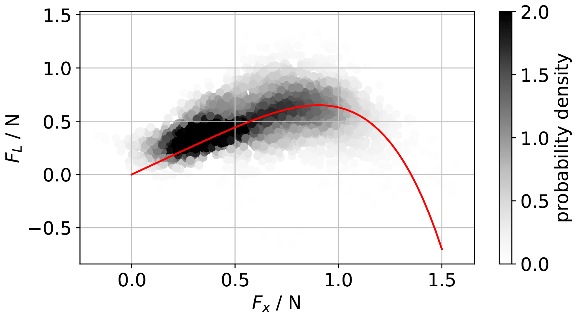
Figure 5Calibration curve of thrust generated by lift FL versus drag force in x direction Fx in the body frame. The greyscale represents the probability of occurrence.
The determined polynomial for the lift correction is
where T0 is a thrust offset value that can depend on changes in UAS mass, changes in motor thrust coefficients, or unmodeled aerodynamic effects.
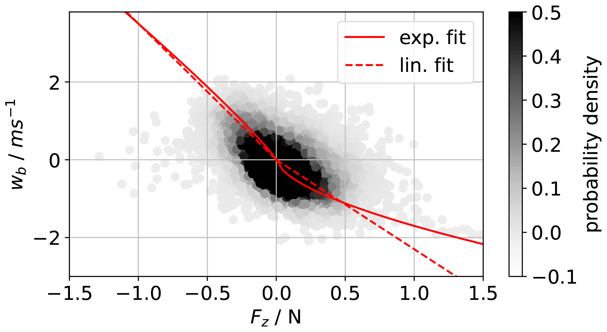
Figure 6Scatterplot of vertical wind of the sonic anemometer versus the acting force on the UAS in the body frame. The greyscale represents the probability of occurrence in the dataset. The solid red line shows the estimated calibration curve. The dashed red line shows a linear fit for comparison.
4.2.2 Thrust offset
We observe that the absolute value of thrust T0 that is needed to maintain altitude in the hovering state varies between single flights and especially between individual UAS. The reasons can be differences in UAS mass, motor performance, or aerodynamic effects. At the present state of development and hardware robustness, we find that T0 needs to be determined in each single flight as the average over the whole flight for best performance. This is justified in flat terrain where zero average vertical velocity can be assumed in most cases. For cases with non-zero vertical velocity, determining T0 from the average over a single flight can yield errors in the absolute value of w but will have little effect on the variance, which is most important for the calculation of TKE and fluxes.
4.2.3 Vertical velocity
In the second step of the calibration, vertical wind is calibrated against thrust (including aerodynamic lift, see above) with data from the FESSTVaL field campaign. Figure 6 shows the scatterplot of all calibration flights of UAS#12. Since measurements of UAS and sonic anemometer are comparatively far apart (≈20 m) and absolute values of vertical wind are rather small, it is not surprising that significant scatter is found in the comparison. It is nevertheless possible to fit a curve according to the theory of Eq. (18). The fitted equation is
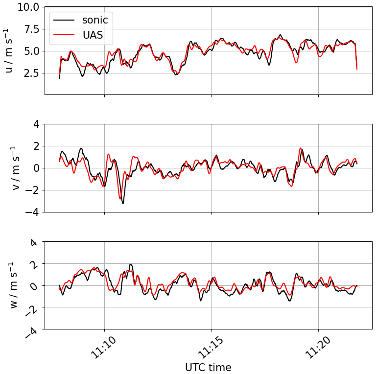
Figure 7Example of time series of u, v, and w for a flight on 2 July 2021 by UAS#13. UAS data (red) are compared to the sonic anemometer at the same height (black).
In comparison to a linear fit, the exponential fit appears to follow the measurements increasingly better for higher negative values of w. However, high absolute values of w are not measured with a high probability.
4.3 Wind vector validation

Figure 8Scatterplots of flight-averaged UAS measurements versus sonic anemometer for u, v, and w (a–c), as well as the corresponding variances (d–f) and covariances (g–i).
The parameters that are determined for UAS#12 are now applied to the whole fleet. We want to compare the wind components u, v, and w in the geodetic coordinate system according to Eq. (13). We rotate the vector horizontally into the main wind direction for both the sonic anemometer and UAS. The coordinate transformation allows us to separate motion around the pitch axis (streamwise) from motion around the roll axis (lateral), which are treated with different calibration coefficients. The wind direction as measured by the UAS is used for the rotation of both UAS and sonic anemometers. The time series in Fig. 7 demonstrates the quality of the wind retrieval in all three dimensions and at a high resolution for a flight in a turbulent ABL with horizontal wind speeds ranging from u=2.5–7.5 m s−1. Figure 8 gives scatterplots of the comparison of flight-averaged wind components; their variances; and the three covariances , , and . Since the wind vector is rotated into the main wind direction during the flight time, the lateral wind component v is zero by definition (Fig. 8b). Flight-averaged vertical velocities are smaller than the uncertainty of the measurement so that a linear regression does not yield a good correlation (p value for test of null-hypothesis P>0.1). The root-mean-square (rms) deviation is . Better parameters to evaluate the quality of the wind retrieval algorithm are the variances of the wind components in lateral and vertical direction. For those, the linear regressions show a very good correlation between UAS and sonic anemometer results (R2>0.9, Fig. 8e, f). The covariance measurements are a good indicator as to whether an independent measurement of horizontal and vertical wind can be guaranteed with the proposed method. The high correlation proves the validity of the method and the rms deviation of approximately for all directions can be considered the prevailing uncertainty of the UAS measurements (Fig. 10g, h). The lower R2 value for is likely due to the imperfect rotation into wind direction for both UAS and sonic anemometer measurements, which introduces larger relative errors for the overall small values. In Fig. A1 we additionally present the validation results in a meteorological wind coordinate system (u is eastward, v is northward, w is up).
4.4 Validation of resolved turbulence scales
A closer evaluation of the resolved turbulence scales by the UAS can be achieved with the analyses of power spectra of the three wind components in comparison to the sonic anemometer. We choose two representative flights of UAS#12, one in low-wind and low-turbulence conditions in the morning of the 26 June (blue), the other in a turbulent convective boundary layer on 2 July (red). The spectra of the three wind components in Fig. 9 show that an inertial subrange of locally isotropic turbulence with a slope of (dashed grey line) can be observed in both cases. For the low-turbulence case, the spectra as measured by the UAS deviates earlier from the curve as measured by the sonic anemometer than in the high-turbulence case. It can be read from the plots that frequencies above 1 Hz and spectral power below can barely be resolved by the UAS but are dominated by noise. This effect is also observed for the cospectra of the wind components (Fig. 10). For conditions with low turbulence, the noise contributions are limiting the resolution of variance and covariance measurements with the UAS. From the noise level, we estimate this limit in resolution for the variances and covariances to , which is almost equal to the root-mean-square error (RMSE) that was determined in Sect. 4.3.

Figure 9Comparison of power spectra of all three wind components between sonic anemometers and UAS.

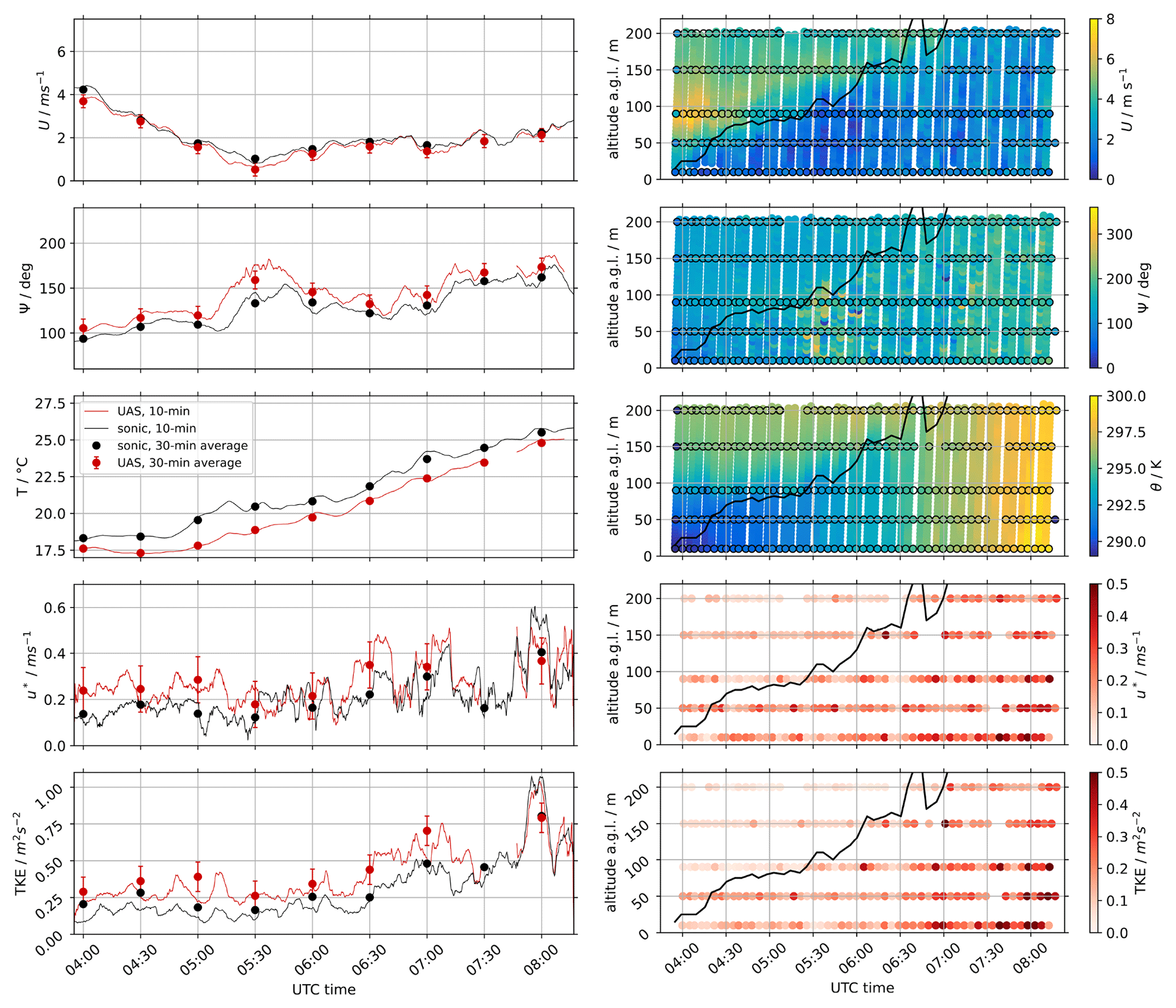
Figure 11Time series of horizontal wind speed U, wind direction Ψ, temperature T, friction velocity u*, and TKE at 50 m above ground level during the morning transition of 28 June 2021 in comparison between UAS and sonic anemometers (left). The continuous lines show 10 min moving averages, whereas the dots give the 30 min mean for each quantity. On the right, Hovmöller diagrams for the observed height range from 10–200 m are shown. The black line indicates the height of the mixed layer below the lowest temperature inversion as observed from vertical profiles of potential temperature θ. For wind speed U, wind direction Ψ, and θ, continuous ascent vertical profiles from a single drone are shown in the background of the measurements from the hovering UAS at 10, 50, 90, 150, and 200 m.
4.5 Momentum flux during a morning transition
A good case to study the validity and capability of the turbulence and flux measurements from the UAS is a transition phase of a convective boundary layer (CBL), which features some significant variability and an increase in turbulence at constant heights. In the morning of 28 June 2021, conditions were present that allowed for the observation of a morning transition of a CBL that was mainly driven by surface heating. In the cloudless night, a stable nighttime inversion had developed, and no clouds were present during the period of observation from 04:00 to 08:00 UTC. A steady increase in shortwave downward radiation from ≈100 to was observed.
Continuous measurements during this period with five stacked UAS at the heights 10, 50, 90, 150, and 200 m were achieved by launching two separate sets of five UAS in turns, with a short overlap of 60 s. The UAS were located close to the meteorological mast as indicated by the blue star in Fig. 3. In total, 23 flights with five UAS each were performed in this pattern. Additionally, a sixth UAS was operating in close proximity (≈5 m apart), profiling the same height range with continuous ascents and descents. The ascents of these flights allow us to obtain profiles of wind speed, wind direction, temperature, and humidity with a high vertical resolution but are not used for the turbulence retrieval. Figure 11 shows the results of the measurements during the morning transition. On the left, the time series of the UAS at 50 m are shown in comparison to the sonic anemometer at the mast at the same level. The data are post-processed with a 10 min moving average for better visualization. Between 07:30 and 07:45 UTC, data are missing because one UAS did not take off as planned. The dots in the plots show the 30 min average with error bars representing the uncertainties that were estimated in Sect. 4.3. We find a good agreement between UAS and sonic anemometer for all variables. The wind direction bias is higher than the determined RMSE from the calibration, especially during those times when the wind speed is lowest. In such conditions, the weather vane controller does not align the UAS very well with the mean wind direction. Around 05:30 UTC, the mixed CBL is growing through the measurement height and wind speed is very weak, and thus the estimation of wind direction deviates by almost 20 ∘ between the UAS and sonic anemometer. In addition, temperature measurements differ most during this period. TKE only picks up significantly after 06:30 UTC, with a large peak just before 08:00 UTC that can be seen in both the UAS and sonic anemometer results. The friction velocity u* is quite variable, also increasing after 06:30 UTC.
In the right column of Fig. 11, Hovmöller diagrams show the transition period in dependency of time and height. From the profiles of potential temperature, an estimate of the boundary layer height as the height of the mixed layer below the lowest inversion is derived and shown as a black line. A low-level jet (LLJ) was present at 100 m above ground level (a.g.l.) that disappears as the mixed layer grows and is the reason for the observed higher wind speeds in the early morning at 50 m and above. It can be clearly seen how low turbulence and high wind speeds above the inversion are separated from low wind speeds and higher turbulence in the mixed layer. Despite the large number of individual UAS that were used to take these measurements (i.e., 12 UAS), no significant biases or discontinuities can be found in the data, which is a good validation of the accuracy of the calibration.
In this work, we present a method to obtain the three-dimensional wind vector with small multicopter UAS. To obtain the vertical wind velocity, motor thrust is included in the equations of motion, and the resulting forces that act on the UAS are calibrated against sonic anemometers to obtain the wind velocity with an rms deviation below 0.2 m s−1 in all three dimensions. We showed that the variance of the wind components can be obtained particularly well with a remaining rms deviation below 0.2 m2 s−2 in all dimensions. The range and limits of the resolvable scales of turbulence are presented with spectra and cospectra of the wind components. It is evident that there is a noise limit in the temporal resolution of approximately 1 Hz and a limit for low-turbulence conditions with spectral power density below . The fact that we could exercise the calibration with a single UAS and apply it to a fleet of more than 20 UAS without a big loss of accuracy shows the robustness of the method and the applicability in practice. From these findings, it can be concluded that UAS of the presented size and weight are capable of resolving eddies of only a few meters. Bigger and heavier UAS will necessarily disturb the flow more, meaning that a small and lightweight design is essential for a high resolution of wind measurements.
In the presented dataset, the range of horizontal wind velocities is limited to . We see that above such wind speeds, aerodynamic effects change, and more studies will be necessary in future to extend the calibration to higher wind speeds. We remove a thrust bias for every individual flight in this study because the assumption of zero average vertical wind speed can be made in the flat terrain in which the experiment was carried out, and this approach will lead to the best estimates of vertical velocity variance. For conditions with a significant average vertical velocity component, different strategies will need to be developed in the future, which may incorporate more robust hardware configurations, an integrated weight estimator in the Kalman Filter, or individual calibration of motor thrusts for UAS. For both constraints, the obtained dataset from the FESSTVaL campaign cannot be used to improve the calibration. In general, calibration with field data is prone to large uncertainties due to the complex ABL flow. The calibration dataset is thus subject to significant scatter, and the polynomials that are used for the relationship between forces and wind speed are not strictly based on physical principles, as simplifying assumptions are made. In the future, we plan to conduct wind tunnel experiments to study the aerodynamic effects in a broader range of horizontal and vertical wind velocities and in more detail. Hardware modifications that allow for hover flights indoors are currently being prepared for this purpose. We are also preparing temperature sensors with a faster response time to be able to measure sensible heat flux in a broad range of atmospheric conditions in the future.
We have shown the potential of multicopter UAS measurements for fundamental ABL research with a case study during a morning transition of a CBL. In this case study, the calibration was applied to 12 individual UAS and a seamless time series over 4.5 h could nevertheless be realized at six measurement heights. The evolution of wind speed and temperature, as well as TKE and shear stress, is well captured in comparison to the reference from sonic anemometers throughout the transition period. This example demonstrates the advantage of operating a fleet of multiple UAS to obtain spatiotemporal in situ data at flexible measurement points throughout the ABL. The possibilities for deploying such a system for ABL studies in complex flow environments such as wind farms or mountainous terrain are numerous, and an observational gap can potentially be closed with this approach.
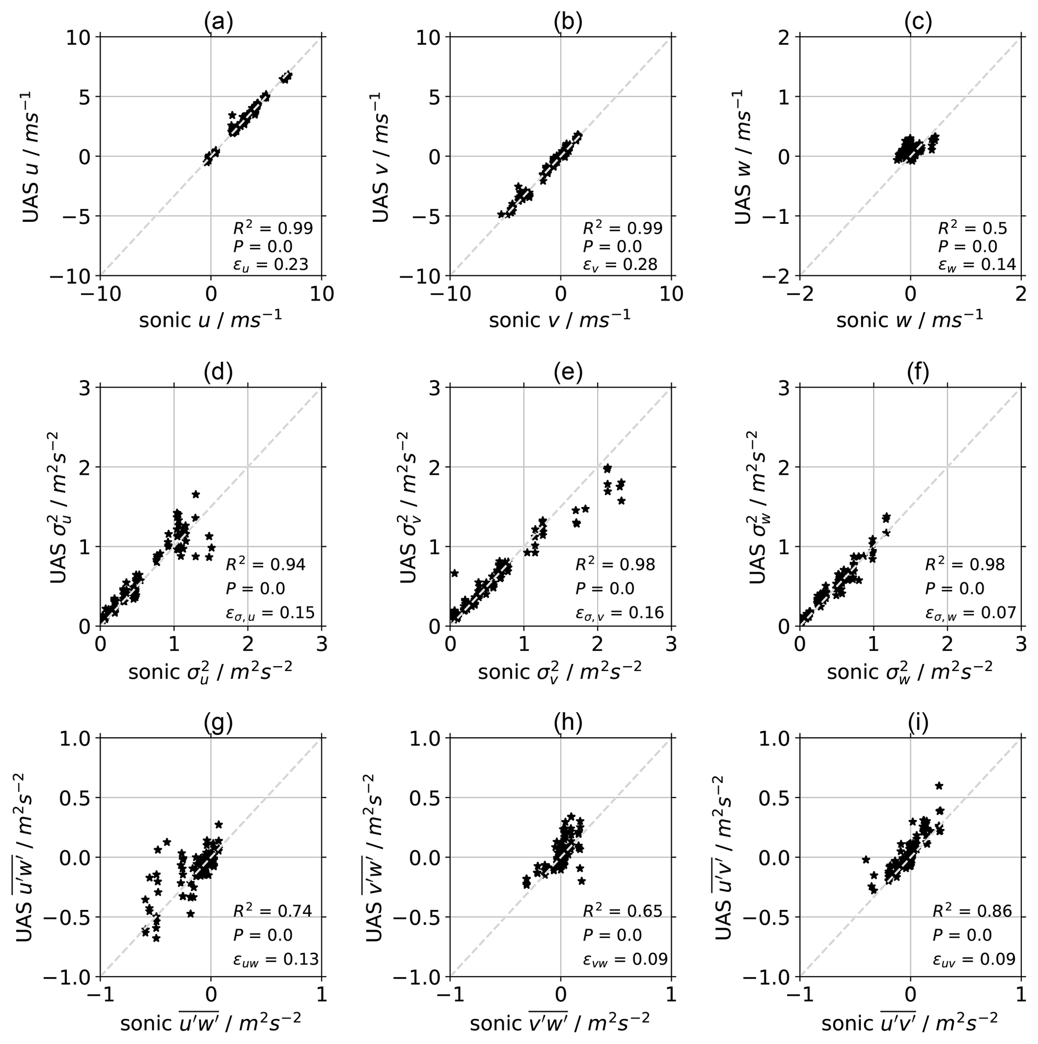
Figure A1Scatterplots of flight-averaged UAS measurements versus sonic anemometer for u, v, and w (a–c), as well as the corresponding variances (d–f) and covariances (g–i) in the meteorological frame of reference.
Both authors jointly developed and carried out the field experiment. NW developed the ideas to retrieve vertical velocity and carried out the motor calibration. TW developed the calibration for horizontal wind speed.
The contact author has declared that none of the authors has any competing interests.
Publisher's note: Copernicus Publications remains neutral with regard to jurisdictional claims in published maps and institutional affiliations.
We acknowledge the support of DWD and the GM Falkenberg provided when we were conducting the experiment. We thank May Bohmann and Josef Zink for their assistance in the execution of the experiments. Many thanks to Frank Holzäpfel for performing an internal review of the manuscript.
The article processing charges for this open-access publication were covered by the German Aerospace Center (DLR).
This paper was edited by Dominik Brunner and reviewed by two anonymous referees.
Aubinet, M., Vesala, T., and Papale, D.: Eddy Covariance – A Practical Guide to Measurement and Data Analysis, Springer, Dordrecht, ISBN 978-94-007-2351-1, https://doi.org/10.1007/978-94-007-2351-1, 2012. a
Baldocchi, D., Falge, E., Gu, L., Olson, R., Hollinger, D., Running, S., Anthoni, P., Bernhofer, C., Davis, K., Evans, R., Fuentes, J., Goldstein, A., Katul, G., Law, B., Lee, X., Malhi, Y., Meyers, T., Munger, W., Oechel, W., U, K. T. P., Pilegaard, K., Schmid, H. P., Valentini, R., Verma, S., Vesala, T., Wilson, K., and Wofsy, S.: FLUXNET: A New Tool to Study the Temporal and Spatial Variability of Ecosystem-Scale Carbon Dioxide, Water Vapor, and Energy Flux Densities, B. Am. Meteorol. Soc., 82, 2415–2434, https://doi.org/10.1175/1520-0477(2001)082<2415:FANTTS>2.3.CO;2, 2001. a
Bangura, M., Melega, M., Naldi, R., and Mahony, R.: Aerodynamics of rotor blades for quadrotors, arXiv preprint arXiv:1601.00733, p. 42, 2016. a
Fernando, H. J. S., Mann, J., Palma, J. M. L. M., Lundquist, J. K., Barthelmie, R. J., Belo-Pereira, M., Brown, W. O. J., Chow, F. K., Gerz, T., Hocut, C. M., Klein, P. M., Leo, L. S., Matos, J. C., Oncley, S. P., Pryor, S. C., Bariteau, L., Bell, T. M., Bodini, N., Carney, M. B., Courtney, M. S., Creegan, E. D., Dimitrova, R., Gomes, S., Hagen, M., Hyde, J. O., Kigle, S., Krishnamurthy, R., Lopes, J. C., Mazzaro, L., Neher, J. M. T., Menke, R., Murphy, P., Oswald, L., Otarola-Bustos, S., Pattantyus, A. K., Rodrigues, C. V., Schady, A., Sirin, N., Spuler, S., Svensson, E., Tomaszewski, J., Turner, D. D., van Veen, L., Vasiljević, N., Vassallo, D., Voss, S., Wildmann, N., and Wang, Y.: The Perdigão: Peering into Microscale Details of Mountain Winds, B. Am. Meteorol. Soc., 100, 799–819, https://doi.org/10.1175/BAMS-D-17-0227.1, 2019. a
Kaimal, J. C. and Businger, J. A.: A Continuous Wave Sonic Anemometer-Thermometer, J. Appl. Meteorol. Climatol., 2, 156–164, https://doi.org/10.1175/1520-0450(1963)002<0156:ACWSAT>2.0.CO;2, 1963. a
Koch, S. E., Fengler, M., Chilson, P. B., Elmore, K. L., Argrow, B., Andra, D. L., and Lindley, T.: On the Use of Unmanned Aircraft for Sampling Mesoscale Phenomena in the Preconvective Boundary Layer, J. Atmos. Ocean. Technol., 35, 2265–2288, https://doi.org/10.1175/JTECH-D-18-0101.1, 2018. a
Leishman, J.: Principles of Helicopter Aerodynamics, Cambridge Aerospace Series, Cambridge University Press, ISBN 9781107013353, 866 pp., 2016. a, b
Mahrt, L.: Flux Sampling Errors for Aircraft and Towers, J. Atmos. Ocean. Technol., 15, 416–429, https://doi.org/10.1175/1520-0426(1998)015<0416:FSEFAA>2.0.CO;2, 1998. a
Mann, J., Kristensen, L., and Courtney, M.: The Great Belt coherence experiment. A study of atmospheric turbulence over water, no. 596(EN) in Denmark, Forskningscenter Risoe, Risoe-R, 1991. a
Mauder, M. and Zeeman, M. J.: Field intercomparison of prevailing sonic anemometers, Atmos. Meas. Tech., 11, 249–263, https://doi.org/10.5194/amt-11-249-2018, 2018. a
Mauder, M., Foken, T., and Cuxart, J.: Surface-Energy-Balance Closure over Land: A Review, Bound.-Lay. Meteorol., 177, 395–426, https://doi.org/10.1007/s10546-020-00529-6, 2020. a
Morrison, T., Pardyjak, E. R., Mauder, M., and Calaf, M.: The Heat-Flux Imbalance: The Role of Advection and Dispersive Fluxes on Heat Transport Over Thermally Heterogeneous Terrain, Bound.-Lay. Meteorol., 183, pages 227–247, https://doi.org/10.1007/s10546-021-00687-1, 2022. a
Segales, A. R., Greene, B. R., Bell, T. M., Doyle, W., Martin, J. J., Pillar-Little, E. A., and Chilson, P. B.: The CopterSonde: an insight into the development of a smart unmanned aircraft system for atmospheric boundary layer research, Atmos. Meas. Tech., 13, 2833–2848, https://doi.org/10.5194/amt-13-2833-2020, 2020. a
Stull, R.: An Introduction to Boundary Layer Meteorology, Kluwer Acad., Dordrecht, ISBN 978-94-009-3027-8, https://doi.org/10.1007/978-94-009-3027-8, 1988. a, b
Thielicke, W., Hübert, W., Müller, U., Eggert, M., and Wilhelm, P.: Towards accurate and practical drone-based wind measurements with an ultrasonic anemometer, Atmos. Meas. Tech., 14, 1303–1318, https://doi.org/10.5194/amt-14-1303-2021, 2021. a
van den Kroonenberg, A. C., Martin, T., Buschmann, M., Bange, J., and Vörsmann, P.: Measuring the Wind Vector Using the Autonomous Mini Aerial Vehicle M2AV, J. Atmos. Ocean. Technol., 25, 1969–1982, 2008. a
Wetz, T. and Wildmann, N.: Spatially distributed and simultaneous wind measurements with a fleet of small quadrotor UAS, J. Phys. Conf. Ser., 2265, 022086, https://doi.org/10.1088/1742-6596/2265/2/022086, 2022. a, b, c, d
Wetz, T., Wildmann, N., and Beyrich, F.: Distributed wind measurements with multiple quadrotor unmanned aerial vehicles in the atmospheric boundary layer, Atmos. Meas. Tech., 14, 3795–3814, https://doi.org/10.5194/amt-14-3795-2021, 2021. a, b, c, d, e
Wildmann, N.: Multicopter UAS measurements at GM Falkenberg during FESSTVaL 2021, Universität Hamburg [data set], https://doi.org/10.25592/UHHFDM.10148, 2022. a
Wildmann, N., Rau, G. A., and Bange, J.: Observations of the Early Morning Boundary-Layer Transition with Small Remotely-Piloted Aircraft, Bound.-Lay. Meteorol., 157, 345–373, https://doi.org/10.1007/s10546-015-0059-z, 2015. a
Wolfe, D. E. and Lataitis, R. J.: Boulder Atmospheric Observatory: 1977–2016: The End of an Era and Lessons Learned, B. Am. Meteorol. Soc., 99, 1345–1358, https://doi.org/10.1175/BAMS-D-17-0054.1, 2018. a