Automatic quality control of telemetric rain gauge data providing quantitative quality information (RainGaugeQC)

The RainGaugeQC scheme described in this paper is intended for real-time quality control of telemetric rain gauge data. It consists of several checks: detection of exceedance of the natural limit and climate-based threshold as well as checking of the conformity of rain gauge and radar observations, the consistency of time series from heated and unheated sensors, and the spatial consistency of adjacent gauges. The proposed approach is focused on assessing the reliability of individual rain gauge observations. A quantitative indicator of reliability, called the quality index (QI), describes the quality of each measurement as a number in the range from 0.0 (completely unreliable measurement) to 1.0 (perfect measurement). The QI of a measurement which fails any check is lowered, and only a measurement very likely to be erroneous is replaced with a “no data” value. The performance of this scheme has been evaluated by analysing the spatial distribution of the precipitation field and comparing it with precipitation observations and estimates provided by other techniques. The effectiveness of the RainGaugeQC scheme was also analysed in terms of the statistics of QI reduction. The quality information provided is very useful in further applications of rain gauge data. The scheme is used operationally by the Polish national meteorological and hydrological service (Institute of Meteorology and Water Management – National Research Institute).

1 Introduction

The accuracy of telemetric rain gauge data is vital for both scientific research and real-time modelling. Reliable precipitation measurements with high temporal and spatial resolution are essential input data for numerous operational applications in meteorology and hydrology, such as quantitative precipitation estimation (QPE), nowcasting, real-time initial conditions for numerical weather prediction, and hydrological modelling. Incorrect values may affect the results of these applications; this especially applies to unreasonably high or false zero precipitation values.

In recent decades, the number of automated weather station networks providing measurements with high temporal resolutions (e.g. 1, 5, or 10 min) has rapidly increased. Consequently, procedures for data quality control (QC) have developed from manual or semiautomatic to fully automatic checks that provide relevant quality information, such as quality flags or quality indices (Lewis et al., 2021). However, in the case of precipitation, the effectiveness of automatic quality control methods has been proven to be much lower than in the case of other meteorological parameters (You et al., 2007). The key issue is that the spatiotemporal variability of the precipitation field, which can be very intermittent and small scale, depends strongly on the type of precipitation (e.g. convective or frontal) and also on topographic variables in mountainous areas with complex terrain (Scherrer et al., 2011).

This paper presents the RainGaugeQC software, which is a package of automatic QC procedures, developed at the Institute of Meteorology and Water Management – National Research Institute (IMGW), which operates the Polish national meteorological and hydrological service. The scheme focuses on telemetric rain gauge measurements and is designed to identify erroneous or suspicious data and to assign a quality index (QI) to the individual measurements. RainGaugeQC was specifically designed for quality control of sub-hourly rain gauge data. This is a particularly challenging task because of the higher spatial variability and lower spatial consistency of such data (Villalobos Herrera et al., 2022).

1.1 Sources of errors in rain gauge data

Ground rain gauge measurements, like other observations, are affected by different types of errors, usually classified as random, systematic, and gross errors. Random errors vary in an unpredictable manner, while systematic errors remain constant or vary in a predictable way and can often be reduced. Gross errors are characterized by rare occurrence and large magnitude (WMO-No. 488, 2017).

Problems relating to the accuracy of precipitation measurement have been well documented (e.g. Sevruk, 1996; Habib et al., 2001; Golz et al., 2005; Sieck et al., 2007; Sevruk et al., 2009). The magnitude of measurement errors depends on many factors, including weather conditions at the collector, the location of the rain gauge, and the gauge type. The most significant measurement errors are related to wind (Sevruk et al., 2009; Rasmussen et al., 2012; Martinaitis et al., 2015). Wind-induced losses mainly depend on wind speed and turbulence, as well as the type of precipitation (e.g. rain, mixed snow and rain, or snow). The measurement error is usually greater for solid than for liquid precipitation (WMO-No. 8, 2018). Because of slow falling, snow hydrometers are more susceptible to deflection by wind-induced turbulence around the gauge, making snowfall measurements prone to large systematic errors (Rasmussen et al., 2012). In windy conditions, the underestimation of snowfall accumulation frequently ranges from 20 % to 50 % or even higher and additionally depends on other variables, such as exposure and the type of rain gauge (Rasmussen et al., 2012; Buisán et al., 2017; Grossi et al., 2017). Other systematic error sources are related to physical processes, such as evaporation from a bucket, wetting, and splashing. All such errors are typically referred to as catching losses.

Additional difficulties occur in winter precipitation measurements as a result of snow collecting on the gauge or snow accumulating within wind shields, either of which can completely or partially block the gauge orifice (Goodison et al., 1998; Rasmussen et al., 2012; Martinaitis et al., 2015; Kochendorfer et al., 2020). In consequence, Martinaitis et al. (2015) identified a secondary but important impact from gauges that had become partially or completely stuck during winter precipitation events. Thawing due to increased surface ambient temperatures resulted in gauges reporting false non-zero precipitation after having collected solid precipitation. These impacts became increasingly complex when rainfall occurred simultaneously with the thawing of accumulated solid precipitation.

Moreover, the accuracy of precipitation measurements may be affected by improper exposure of the gauge, site altitude, shielding or obstacles (e.g. trees, buildings) near the rain gauge, the impact of topographic variables in complex areas, and the seeder–feeder effect when precipitation from an upper-level cloud falls through a lower-level orographic stratus cloud capping a small mountain (Førland et al., 1996; Sevruk and Nevenic, 1998).

Additionally, mechanical problems specific to each type of rain gauge influence the accuracy of precipitation measurements. Tipping bucket rain gauges are subject to random errors related to partial or total blockages of the mechanism due to accumulated mineral or biological particulate such as dust, insects, and blown grass (Sevruk, 1996; Upton and Rahimi, 2003). In consequence, even partial clogging of the gauge can result in erroneous estimates of the intensity and duration of rainfall. Another specific problem with tipping bucket rain gauges relates to high-frequency bucket tips (double tips), which lead to the recording of spurious high rainfall intensities, while on the other hand very slow tips (i.e. a limited tipping rate) may result in misleading underestimates of rain rates (Upton and Rahimi, 2003; Shedekar et al., 2016).

In the case of weighing gauges, the most relevant sampling errors are related to the response time of the measurement system and the consequent systematic delay in assessing the exact weight of the accumulated precipitation in the container, especially in the case of high resolution (e.g. a 1 min time resolution). Sampling errors may also affect the measurement of low-intensity rain (Colli et al., 2013).

Electronic weighing precipitation gauges are less susceptible to evaporation losses than tipping bucket gauges and have better accuracy in assessing the beginning of snowfall events. A heated tipping bucket gauge starts recording with a delay due to the time needed to melt the snow and fill the first tip, and it measures less precipitation due to heating-related losses (Savina et al., 2012).

Furthermore, precipitation measurements may be affected by gross errors, mainly caused by the malfunctioning of measurement devices or occurring during data transmission.

1.2 Approaches to quality control of rain gauge data

Quality control is a vital part of data processing in order to achieve a certain standard for international data exchange. The World Meteorological Organization (WMO) recommends initially performing real-time basic QC of raw data at sensor level, then near-real-time QC, and finally non-real-time extended QC (semiautomatic) at the headquarters (WMO-No. 488, 2017). Performing QC at various stages of data processing makes it possible to identify the majority of errors in the dataset.

Generally speaking, some precipitation data QC checks consider each single observation separately (Upton and Rahimi, 2003; Taylor and Loescher, 2013; Blenkinsop et al., 2017), whereas more complex ones also take into account data from neighbouring stations (Steinacker et al., 2011; Scherrer et al., 2011) or multi-source data, such as weather radar data (Yeung al., 2014; Baserud et al., 2020) and output from a numerical weather prediction model (Qi et al., 2016). Recently, due to the increased utilization of crowdsourced observations, specific QC methods applicable for this type of precipitation data have been developed (de Vos et al., 2019; Bárdossy et al., 2021; Niu et al., 2021).

For assessing the reliability of observations, several approaches are adopted. In practice, various measures of the quality of precipitation data are used. They indicate the reliability of individual sensors resulting from measurement precision, which is strongly conditioned by construction and technology (Førland et al., 1996), location, and current meteorological conditions (wind, temperature), among other factors. Often, flags describing the quality of the data are used qualitatively; for example, the WMO recommends a scheme of five quality flags, defined as good, inconsistent, doubtful, erroneous, and missing (WMO-No. 488, 2017, p. 201).

In the simple approach to QC outputs, the only possible result is the acceptance or rejection of particular observations. An observation that passes all of the checks is flagged as correct. If an observation fails a check, it is flagged as incorrect and does not undergo the remaining checks (Baserud et al., 2020); however, it is possible to retrieve information on which test was failed for each observation. Some QC schemes integrate the results of individual QC checks to generate a final flag for each observation. In this case an adjustment test or specially designed rule base is applied to minimize the number of correct observations that are flagged as “erroneous”. For example, if an observation failed a climate-based range test but passed the spatial check, then an adjustment test may reduce the severity of the flag obtained from the climate-based range check (Fiebrich et al., 2010; Lewis et al., 2018, 2021).

In another approach, after failing specific checks the measured values are not removed, but corrected. Such a method may be used to replace suspicious data with values obtained from interpolation data from neighbouring stations (Michelson, 2004), but it does not provide any additional information. Also, the use of data from other measurement systems is not a satisfactory solution, as these data are generally inconsistent with each other due to their different spatial distributions. Generally, the correction of measured values can give unreliable results due to the high level of arbitrariness.

Recently, machine learning using artificial neural networks has been employed as a tool for automated quality control as well as for the correction of errors and reconstruction of missing values in precipitation data (Moslemi and Joksimovic, 2018).

Quantitative indicators describing the quality of the observations can also be used, most often as a quality index (QI) ranging from 0.0 for completely unreliable measurement to 1.0 for perfect measurement (Einfalt et al., 2010; Szturc et al., 2022). This approach is adopted in the QC scheme described in this paper. In the developed RainGaugeQC scheme, the quality of uncertain measurements is lowered and only measurements very likely to be erroneous are removed – they are replaced with “no data” values. The advantage of this approach is that the quality information can be very useful in further applications. For example, it is employed in quality-based spatial interpolation of rain gauge data and in merging observations from different measurement techniques (e.g. Jurczyk et al., 2020). It seems optimal to take into account quantitative information about the quality of individual measurements in such a way that the more uncertain data are assigned a lower weight than more reliable data.

1.3 Structure of the paper

The paper is structured as follows. After Sect. 1, Sect. 2 briefly describes the rain gauge data on which the RainGaugeQC scheme proposed in the paper was developed and calibrated, as well as the radar data used as auxiliary data in this scheme. In Sect. 3, the checks that constitute the RainGaugeQC system are presented (their detailed descriptions are included in the Appendices). Section 4 presents and discusses specific examples of the scheme's performance and a general analysis of its operation. The article ends with a list of conclusions resulting from the operational use of the RainGaugeQC scheme at IMGW (Sect. 5).

2 Data sources

2.1 Rain station network in Poland

The Polish national meteorological and hydrological service, provided by IMGW, operates a nationwide meteorological telemetric network which consists of 503 rain stations equipped mainly with tipping bucket sensors (Fig. 1). At the synoptic stations, SEBA Hydrometrie (https://www.seba-hydrometrie.com/, last access: 27 September 2022) RG-50 devices are installed, whereas precipitation stations mainly use Met One Instruments (https://metone.com/, last access: 27 September 2022) 60030 and 60030H devices (unheated and heated, respectively). Telemetric precipitation measurements are available with a 10 min time resolution: all year round for heated sensors and in the warm part of the year – from April to October – for unheated ones.

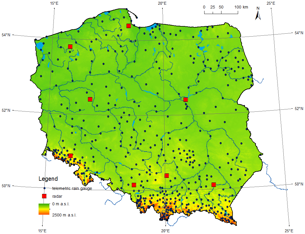
Figure 1 Networks of telemetric rain stations and weather radars in Poland.

The reliability of individual rain gauge depends on the type of the gauge and its location, and it changes with time. The network's tipping bucket devices often malfunction, and moreover these sensors lower the precipitation values by an average of about 8 %–20 % (Urban and Strug, 2021).

Figure 2 shows the relationships between measurements of 10 min precipitation accumulation from unheated and heated sensors at two sample rain stations: in Dzierżoniów, located in the foothills area, during July 2021 (left) and in Nowa Wieś Podgórna, located in the lowland Wielkopolska (Greater Poland) region in central Poland, during June 2021 (right). Both stations are equipped with two tipping bucket sensors. The following denotations are introduced for the precipitation values they measure: G_h is the 10 min precipitation amount observed by the heated sensor, and G_uh is the analogical value observed by the unheated one. The correlation coefficient calculated for pairs of values in which at least one is different from zero is extremely high for Dzierżoniów, being equal to 0.997 (Fig. 2a), while for Nowa Wieś Podgórna it is only 0.694 (Fig. 2b), which is a fairly low result caused by very large differences between the values measured simultaneously by the two sensors at the same location. The reason for such low correlation may be that tipping bucket gauges are susceptible to frequent sensor failures.

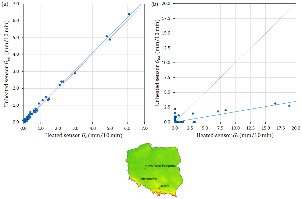
Figure 2 Relationships between observations of 10 min precipitation accumulation measured with tipping bucket rain stations equipped with two sensors – unheated and heated – in Dzierżoniów during July 2021 (a) and in Nowa Wieś Podgórna during June 2021 (b). The blue lines mark the trends of these relationships. The data from three rain stations shown in the bottom map are discussed in the examples.

Generally, the left graph of Fig. 2 corresponds to a well-functioning rain station, and the right graph corresponds to a rain station with one or both sensors not functioning correctly. Therefore, they require effective quality control. It is shown in Sect. 4.3, concerning an example case study, how the quality control scheme presented in this paper worked on these obviously incorrect measurements.

2.2 Weather radar data

Weather radar data are employed in the RainGaugeQC scheme as auxiliary data to verify rain gauge observations. They are generated by the Polish radar network POLRAD, which consists of eight C-band Doppler radars from Leonardo Germany GmbH (formerly Gematronik and Selex; Szturc et al., 2018). Three of them are dual-polarization radars, and work is currently underway on upgrading all the radars, including dual-polarization functionality. Three- and two-dimensional radar products are generated by Rainbow 5 software every 10 min, with a 1 km spatial resolution within a 215 km range. The Marshall–Palmer formula is used to transform the reflectivity values measured by radar into the precipitation rate, this being the most common form of such a relationship (Neuper and Ehret, 2019). The data are quality-controlled by the dedicated RADVOL-QC system developed at IMGW (Ośródka et al., 2014; Ośródka and Szturc, 2022). The system also generates quality fields, QI(R), based on analyses of particular errors disturbing radar data.

2.3 Other data

In addition, the fields of the following precipitation estimates were used for the case studies:

• satellite precipitation fields determined from various NWC-SAF (Satellite Application Facilities on Support to Nowcasting and Very Short Range Forecasting) products based on Meteosat data (Jurczyk et al., 2020);

• QPE fields produced by the RainGRS system, which operationally combines precipitation data from rain gauges, weather radar, and meteorological satellites based on conditional merging and additionally taking quality information into account (Jurczyk et al., 2020).

3 General description of the developed quality control scheme

3.1 Set of RainGaugeQC algorithms

A shortened version of the description of the algorithms used in the scheme is presented in works by Otop et al. (2018) and Jurczyk et al. (2020). This section and the related Appendices provide a full description of the developed algorithms. All parameters defined here were optimized for 10 min precipitation accumulation (mm/10 min).

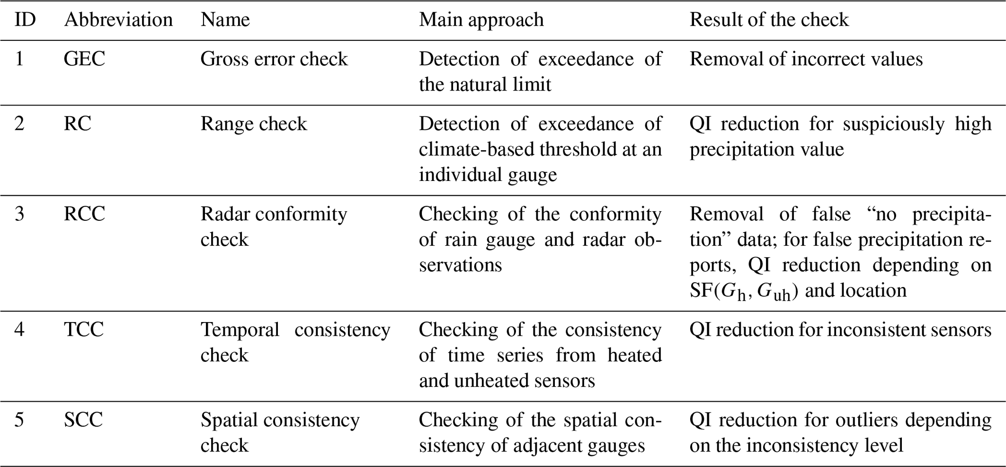
The rain gauge quality control procedure developed at IMGW consists of several checks (Table 1). Firstly, simple plausibility tests – the gross error check and range check – are performed on a single measurement. Then more complex checks are performed using data from both measurement sensors at the site and data from weather radars.

Table 1 List of sequential checks for precipitation QC.

Before the checks, each sensor is assigned the perfect QI value (1.0). In the case of failure of a particular check, the QI value is decreased by a specified value. If the final QI value (after all of the checks) is very weak (≤0.0), the sensor is considered useless and the measurement value is replaced with no data.

The sensor which obtained a higher final quality index is used for further applications, but if both sensors are of the same quality, then the heated sensor is taken.

3.2 Similarity function (SF)

It is useful to introduce a tool to check the similarity of two sums of precipitation. For this purpose a similarity function (SF) has been proposed and is used in some of the checks. The function SF(G_h,G_uh), comparing precipitation data from two sensors G_h and G_uh (heated and unheated) installed at the same rain station G in order to check whether the measured values are consistent, is defined as follows:

$$\begin{array}{}\text{(1)}& \begin{array}{rl}\mathrm{If}& \left(G_{\mathrm{h}}<\mathrm{1.0}\mathrm{mm}\mathrm{or}{G}_{\mathrm{uh}}<\mathrm{1.0}\mathrm{mm}\right),\mathrm{then}\mathrm{if}\\ & \left(\left|G_{\mathrm{h}}-G_{\mathrm{uh}}\right|<\mathrm{1.0}\mathrm{mm}\right),\mathrm{then}\mathrm{SF}\left(G_{\mathrm{h}},G_{\mathrm{uh}}\right)\\ & =\mathrm{`}\mathrm{`}\mathrm{true}\text{”}\mathrm{else}\mathrm{SF}\left(G_{\mathrm{h}},G_{\mathrm{uh}}\right)=\mathrm{`}\mathrm{`}\mathrm{false}\text{”},\end{array}\end{array}$$

whereas

$$\begin{array}{}\text{(2)}& \begin{array}{rl}\mathrm{If}& \left(G_{\mathrm{h}}\ge \mathrm{1.0}\mathrm{mm}\mathrm{and}{G}_{\mathrm{uh}}\ge \mathrm{1.0}\mathrm{mm}\right),\mathrm{then}\mathrm{if}\\ & (\mathrm{0.5}<{\displaystyle \frac{G_{\mathrm{h}}}{G_{\mathrm{uh}}}}<\mathrm{2.0}\mathrm{or}\left|G_{\mathrm{h}}-G_{\mathrm{uh}}\right|<\mathrm{1.0}\mathrm{mm}),\\ & \mathrm{then}\mathrm{SF}(G_{\mathrm{h}},G_{\mathrm{uh}})=\mathrm{`}\mathrm{`}\mathrm{true}\text{”}\\ & \mathrm{else}\mathrm{SF}\left(G_{\mathrm{h}},G_{\mathrm{uh}}\right)=\mathrm{`}\mathrm{`}\mathrm{false}\text{”}.\end{array}\end{array}$$

In the above formulae, precipitation units are given in millimetres (mm), but they may refer to different accumulation periods: for example millimetres per 10 min (mm/10 min) or 1 h.

The result of the use of SF to assess the similarity of measurements between two sensors (heated and unheated) in rain stations is presented in Fig. 3. The graph shows example data for one day, 22 May 2019, obtained from all measuring stations. It is indicated which measurements from the two sensors are shown by the SF to be similar (marked blue) and which are not similar (marked brown). The two blue dashed lines delimit the area in which the values measured by the unheated and heated sensors are similar according to the SF.

Figure 3 Precipitation data from G_uh and G_h sensors that are similar (blue) and not similar (brown). The similarity of the measurements from all rain stations on 22 May 2019 was determined using the similarity function (SF). The two dashed lines delimit the area in which the measurements are considered similar.

3.3 Gross error check (GEC)

GEC is a preliminary check to identify gross errors which have a strong effect on the further analyses. These errors are mainly caused by the malfunctioning of measurement devices or by mistakes occurring during data transmission or processing (Steinacker et al., 2011). GEC examines whether the rain gauge measurement is within the physically acceptable range limits: not less than 0 mm and not above 56 mm/10 min (i.e. 51 dBZ). The upper limit was determined on the basis of a formula developed to estimate the maximum reliable precipitation for various durations in Poland (Burszta-Adamiak et al., 2019). A measurement that fails the check is rejected from further processing.

3.4 Range check (RC)

RC verifies a single measurement against a threshold value, which is based on local climatological data with respect to seasonal variation of observations in the specific location of the rain station. This test identifies data as implausible when they exceed the expected maximum value: that is, the threshold empirically estimated from long-term climatological data. It is essential to ensure reliable values of the threshold because, for example, too low a threshold may cause extreme values of precipitation to fail the test (Taylor and Loescher, 2013). Therefore, Fiebrich et al. (2010) recommend developing regionally specific thresholds for the test. In the proposed QC procedure, the thresholds were defined as 10 min precipitation values with a 1 % probability of being exceeded, determined separately for warm and cold seasons. These values were calculated for each telemetric station based on the statistical distribution of 10 min accumulations in a 30-year time series (1986–2015). In the case that the examined measurement exceeds the relevant threshold value, it is treated as suspicious and its QI is reduced by 0.25.

3.5 Radar conformity check (RCC)

RCC is performed to identify false precipitation – false zero and false gauge-reported precipitation measurements – on the basis of radar data, which quite reliably indicate the spatial distribution of precipitation. RCC compares each gauge observation lower than 0.2 mm/10 min with radar observations at the gauge location and its surrounding of 3 ×3 pixels (the pixel size is 1 km × 1 km). If the radar data for the vicinity of the station are above a predefined threshold, then a “no precipitation” result measured by the sensor is assumed to be false and the QI is reduced to 0.0.

On the other hand, the RCC compares every sensor observation G>0 mm/10 min with radar observations at the gauge location and its neighbouring of 3 ×3 pixels. If the radar data are of a quality QI(R) above a predefined threshold and indicate no precipitation (0 mm), then the precipitation measured by the sensor is assumed to be false and the QI of that observation is reduced. The reduction depends on whether data are available from one or two sensors, on their similarity, and on the gauge location. The following regions based on altitude are distinguished: lowlands (areas below 300 m a.s.l.), foothills (between 300 and 600 m a.s.l.), and mountainous (areas above 600 m a.s.l.).

For a detailed description of the RCC algorithm and the criteria for determining the reduction of QI, see Appendix A.

3.6 Temporal consistency check (TCC)

This check, in the form described below, is possible only when two sensors are installed at each measuring station, most often heated and unheated, as is currently the case in the IMGW network. If this is not the case, then a method commonly used in quality control of various meteorological quantities is to check the time continuity of the measured values. For some types of meteorological data the time consistency checks are efficient; however, in the case of precipitation data, this check would eliminate not only all questionable data but also a large amount of true data, in particular extreme values because of the high variability of precipitation (WMO-No. 305, 1993, pp. VI.21 and VI.23).

The first step of this check is performed to detect a clogged sensor, which occurs if the same value is repeated over a certain period of time. In this case, the sensor's quality is reduced to 0.0.

In the next step, pairs of rain gauge sensors (G_h, G_uh) are tested for the existence of large differences between them. This check requires measurements from both rain gauge sensors at the same location and can thus be conducted only in the warm half of the year because only then are two time series from the same station available. In this procedure, if the number of measurement pairs is sufficient, they are accumulated and their similarity is checked using the SF (see Sect. 3.2). If the sums differ, the data from both sensors have failed the TCC and their quality is reduced.

For a detailed description of the TCC algorithm see Appendix B.

3.7 Spatial consistency check (SCC)

SCC is applied to identify outliers based on a comparison with neighbouring stations. Additionally, radar data are introduced to assess the level of QI reduction for outliers.

There are several steps in the operational procedure for SCC. Firstly, the domain area is divided into basic subdomains with a spatial resolution of 100 km × 100 km. For each subdomain, a set of percentiles of rain gauge data and the median absolute deviation (MAD) are calculated.

The criterion for the spatial consistency of an individual sensor is implemented based on the index D, calculated using the formula of Kondragunta and Shrestha (2006). This index is compared with the threshold values defined by a set of percentiles of the index D, making it possible to determine the different classes of outliers. The check is repeated for subdomains obtained by making shifts of 25 km in all four directions. If the sensor value is identified as an outlier in the basic subdomain and in the shifted subdomains, the sensor is detected as an outlier and a further procedure is applied to assess the relevant quality reduction.

For each detected outlier, two criteria are checked: (i) if data from both sensors are available for a given rain gauge and they are similar, i.e. SF (G_h, G_uh) is “true” and (ii) if the data passed the TCC test. If both criteria are met, then the QI for the sensor is not reduced. Otherwise, for additional verification, radar data in a grid of 5 ×5 pixels around the gauge location are considered if they are of good quality. In this case the reduction of the QI value depends on the class of the outlier (weak, medium, or strong) and the magnitude of the disparity with the radar data (the limitation imposed on the magnitude of this disparity has been empirically determined).

A detailed description of the SCC algorithm and the criteria for reduction of the QI value are given in Appendix C.

The check may optionally analyse data from both sensors together or separately and may or may not include data from the previous time step. It was investigated how these two settings influence the performance of the check.

Figure 4 presents graphs showing the percentage of data with reduced QI values as a result of analysing the spatial conformity of data from two types of sensors (unheated and heated) separately or together. The obtained sample results generally showed large variation; however, the numbers of strong outliers increased significantly (about 2.35 % versus 0.6 %) when the two types of sensors were analysed separately – in that case the algorithm appears much less tolerant.

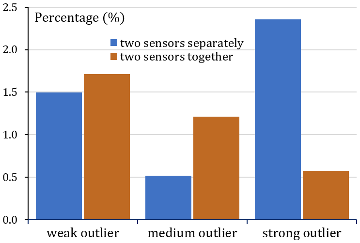
Figure 4 Percentage of classes of outliers (weak, medium, and strong) when analysing the data from two types of sensors (unheated and heated) separately (blue) or together (brown). Data from 22 May 2019.

If the algorithm takes into account data not only from the current time step, but also from 10 min ago (both sensors analysed together), then these numbers are slightly higher for weak and medium outliers and slightly lower for strong ones. The latter indicates that the inclusion of data from the previous time step makes the algorithm more tolerant. The percentage of the data belonging to all classes of outliers together was slightly over 3 % (Fig. 5), and for particular classes it varies from about 1.5 %–1.7 % for the weak to about 0.6 %–0.9 % for the strong outliers.

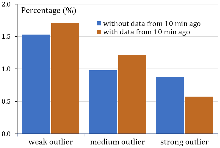
Figure 5 Percentage of classes of outliers (weak, medium, and strong) when analysing measurements from the given time only (blue) and also from the previous time step (brown). Data from two days: 20 and 21 June 2020.

In the RainGaugeQC scheme currently used by IMGW in real time, in the SCC both types of sensors are analysed together, also taking account of the data from the previous time step.

3.8 Quality index of spatially distributed rain gauge data

In most applications of rain gauge data, spatial interpolation of the point data is required and this procedure can be carried out by any of a number of commonly known methods. However, it is not enough to spatially interpolate the QI values assigned to individual rain gauges. It is also necessary to take into account the fact that the uncertainty of the estimated field increases very quickly with increasing distance from the nearest rain gauge. Therefore, the quality field for the spatially distributed precipitation data depends on two factors: the QI point values for individual rain gauges (denoted by the QI with the index p) and a factor that depends linearly on the distance from the nearest rain gauge (with the index d).

The precipitation and QI point values from rain stations are spatially interpolated simultaneously by the same method using the same parameters, so in both cases there are the same contributions from the individual rain gauges. Hence, the obtained quality field QI${\left(G_{\mathrm{int}}(x,y)\right)}_{\mathrm{p}}$ is completely consistent with precipitation field (G_int(xy)). In the case of the operational scheme used by IMGW, ordinary kriging is applied, whereby the domain of 900 km ×800 km is divided into 16 subdomains of 225 km ×200 km and interpolation is performed separately in each of them.

The factor related to the distance from the rain gauges QI${\left(G_{\mathrm{int}}(x,y)\right)}_{\mathrm{d}}$ takes into account the decrease in the quality of the rainfall field depending on the distance d(xy) to the nearest rain gauge. The distance factor for each pixel is calculated from the linear formula

$$\begin{array}{}\text{(3)}& \mathrm{QI}{\left(G_{\mathrm{int}}(x,y)\right)}_{\mathrm{d}}={\displaystyle \frac{d_{\max }-d(x,y)}{d_{\max }}},\end{array}$$

where d_max is the limit value of the distance to the nearest rain gauge, above which the quality at that pixel is assigned a value of zero (the adopted limit is 100 km).

The field of the final quality index for the rain-gauge-based precipitation field is calculated from the product of the two above factors:

$$\begin{array}{}\text{(4)}& \mathrm{QI}\left(G_{\mathrm{int}}(x,y)\right)=\mathrm{QI}\left(G_{\mathrm{int}}(x,y)\right){}_{\mathrm{p}}\cdot \mathrm{QI}\left(G_{\mathrm{int}}(x,y)\right){}_{\mathrm{d}}.\end{array}$$

4 Examples of QC scheme operation

4.1 Influence of differences in values from two sensors on precipitation field estimation

In the example presented in Fig. 6, it can be seen that the data from the two sensors can sometimes be significantly different. In simpler solutions the final rainfall field can be generated by taking the mean or the higher values of the two sensors at the same location, and both of these approaches can be justified depending on the final application of the data. The approach used in the RainGaugeQC scheme makes it possible to choose the better value according to defined checks. Moreover, it enables applying that precipitation value along with the relevant QI value in quality-based interpolation algorithms which generate the optimal rain gauge field.

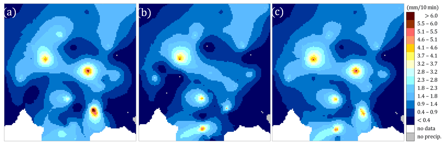
Figure 6 Spatially interpolated rain station data obtained from (a) unheated and (b) heated sensors, as well as (c) after quality control (considered optimal). Data from 5 August 2021 at 17:40 UTC for a fragment of the Polish domain (240 km ×250 km).

4.2 Result of the performance of the QC scheme after the introduction of erroneous values

Figure 7 illustrates the performance of the proposed QC scheme. If the rain gauge data are not subjected to QC algorithms, then two alternative datasets can be considered: from unheated (Fig. 7a) and heated (Fig. 7b) sensors. The third diagram shows an example of data disturbed with an artificial value of 10 mm/10 min at the heated sensor of the Siercza rain station (Fig. 7c), which is marked with a red circle in all diagrams. The location of the Siercza rain station is shown in Fig. 2 (bottom).

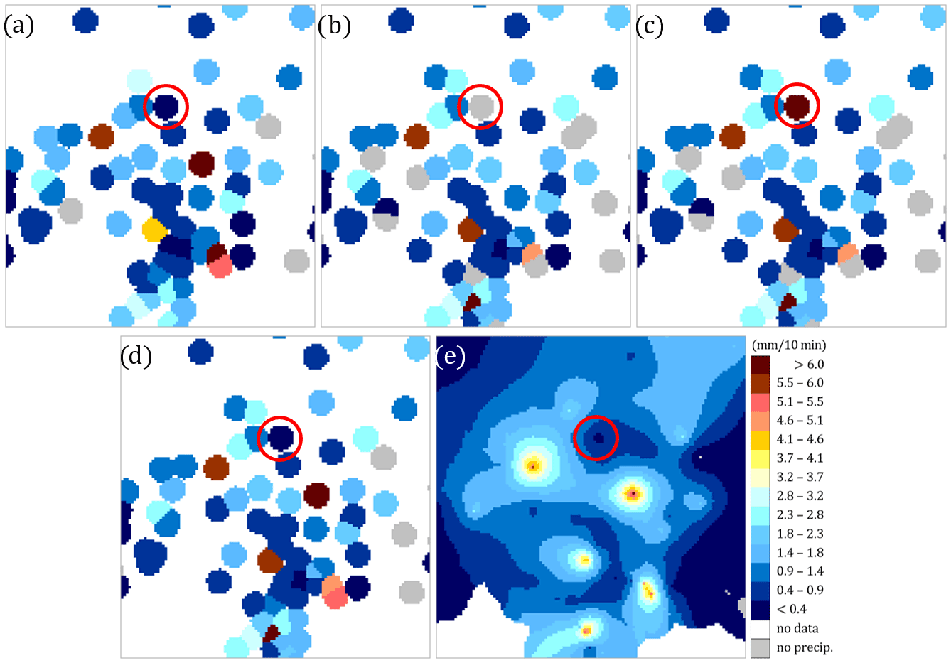
Figure 7 Example of the RainGaugeQC performance after the introduction of an erroneous precipitation value: (a) original rain gauge data from unheated sensors (G_uh; in all fields the Siercza rain station is marked with a red circle), (b) original data from heated sensors (G_h), (c) data from heated sensors disturbed with an artificial value at Siercza (10 mm/10 min), (d) rain gauge data after quality control, and (e) data after spatial interpolation. Data from 5 August 2021 at 17:40 UTC for a fragment of the Polish domain (240 km ×250 km).

Figure 7d shows the values from individual rain stations after quality control, and Fig. 7e shows the precipitation field after spatial interpolation using the ordinary kriging technique (this field is identical to the one shown in Fig. 6c). As these images show, the precipitation values obtained after data quality control are some mixture of those data from both sensors that passed the QC with higher QI (see Sect. 3.1). The Siercza rain station, marked with a red circle, serves here as an example of a station with incorrect measurement (the original values were 0.2 and 0.0 mm/10 min for unheated and heated sensors, respectively). The erroneous value of 10 mm/10 min was eliminated as a result of the QC algorithms, so the rainfall value for this rain station after QC is 0.2 mm/10 min measured by the unheated sensor.

4.3 Example for Nowa Wieś Podgórna rain station from 22 June 2021, 13:30 UTC

An example of a rain station with low-quality measurements, taken from the Nowa Wieś Podgórna rain station during June 2021, is shown in Fig. 2b (Sect. 2.1). The low quality is evidenced by large differences between the values measured with heated and unheated sensors: the heated sensor recorded much higher 10 min precipitation accumulation than the unheated one. The data from 22 June 2021 at 13:30 UTC are analysed in detail below. The heated sensor of the Nowa Wieś Podgórna rain station reported very high rainfall of 18.9 mm/10 min, whereas the unheated one reported only 2.7 mm/10 min (Table 2). If QC is not performed, then the heated sensor is generally considered the primary sensor as it operates all year round. The precipitation field resulting from the interpolation of rain gauge data without QC obtained by the ordinary kriging method is shown in Fig. 8a.

Table 2 Results of QC of the Nowa Wieś Podgórna rain station on 22 June 2021 at 13:30 UTC.

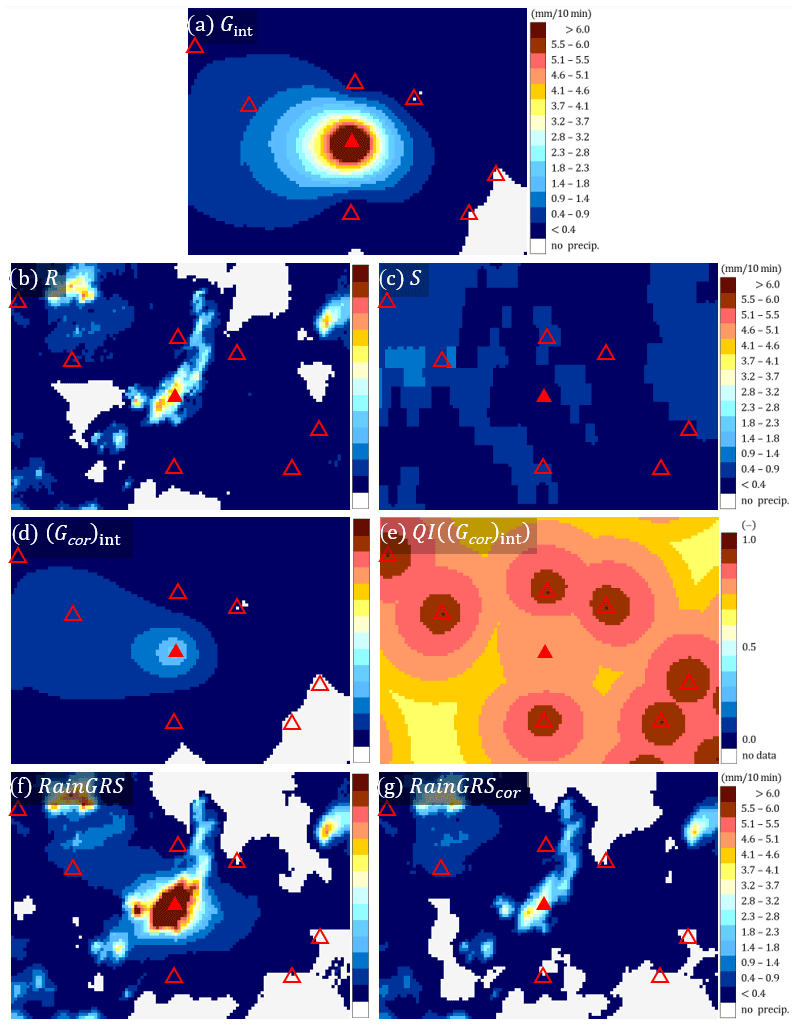
Figure 8 Various fields of 10 min precipitation accumulation (in mm/10 min) in the vicinity of the Nowa Wieś Podgórna rain station (marked with a red triangle; the locations of other rain stations are marked with empty triangles): (a) spatially interpolated field from rain gauge data without QC (G_int), (b) radar-based precipitation field (R), (c) satellite-based precipitation field (S), (d) spatially interpolated field from rain gauge data after QC $\left({\left(G_{\mathrm{cor}}\right)}_{\mathrm{int}}\right)$, (e) QI field for the precipitation field from rain gauge data after QC $\left(\mathrm{QI}\left({\left(G_{\mathrm{cor}}\right)}_{\mathrm{int}}\right)\right)$, (f) multi-source precipitation field (RainGRS) obtained from raw rain gauge data, and (g) multi-source precipitation field (RainGRS_cor) obtained from rain gauge data after QC. Data from 22 June 2021 at 13:30 UTC for a fragment of the Polish domain (110 km ×80 km).

In order to diagnose the large difference between the two sensors, a detailed investigation of the situation was performed based on precipitation data from other sources. The radar composite map from the SRI (surface rainfall intensity) product showed 3.95 mm/10 min at this location (Fig. 8b), which is much closer to the value from the unheated sensor. Satellite rainfall, determined from various NWC-SAF products based on Meteosat data (see Sect. 2.3), showed only 0.05 mm/10 min (Fig. 8c); however, measurements based on data from visible and infrared channels are much less accurate than radar measurements. The radar data confirmed that the rainfall that occurred in the analysed time step in the close vicinity of this rain station is significantly higher than in the surroundings, but not by as much as the heated sensor reported – it is much closer to the observation of the unheated sensor.

Visually, this conclusion seems to be unquestionable, but it may be interesting how the designed RainGaugeQC scheme functioned in this situation.

Figure 9 shows the recorded precipitation time series from 12 time steps (i.e. 2 h) before the analysis date (13:30 UTC) and 6 time steps after this date at Nowa Wieś Podgórna station (two sensors) as well as maximum values of the four neighbouring stations. These stations are located between 19 and 35 km from the analysed Nowa Wieś Podgórna station. Until the analysis date, precipitation measured by the sensors of these stations was not high, as it was up to about 1 mm/10 min, but 20 min later a significant increase in precipitation of about 6 mm/10 min was observed on both sensors of one of the nearby stations. At the analysed time step only Nowa Wieś Podgórna station recorded slightly higher precipitation on the heated sensor, while it was drastically higher on the unheated sensor (Table 2).

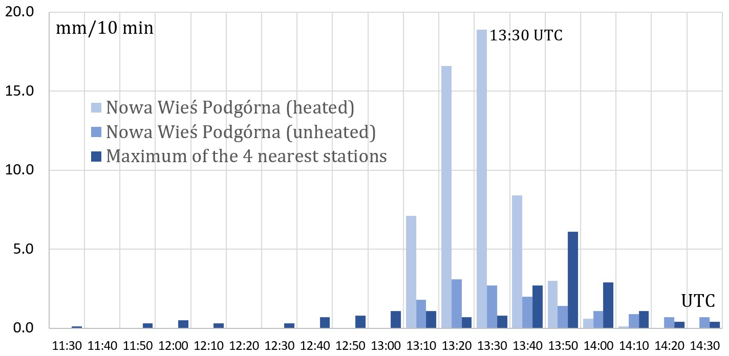
Figure 9 Precipitation time series at Nowa Wieś Podgórna station in comparison to the maximum of four neighbouring rain stations on 22 June 2021 from 11:30 to 14:30 UTC.

The quality of the data from this rain station was 0.75 for the G_uh sensor and 0.50 for G_h. This difference in QI values was a result of the SCC test, which showed that the G_uh sensor differs slightly and the G_h sensor differs significantly from the rainfall values in the neighbouring rain stations within the given subdomain. At the same time, both sensors failed the TCC test, which in turn indicates that the accumulated values measured by these two sensors over the last 12 time steps differ significantly (Table 2). This also contributed to a reduction in the final QI value.

Thus, finally, the value from the unheated sensor G_uh is taken for further processing. The precipitation field after the spatial interpolation of QC data obtained by the ordinary kriging method is shown in Fig. 8d. The precipitation values around this rain station location are clearly lower than those shown in Fig. 8a (without QC). The QI field for spatially interpolated rain gauge data is shown in Fig. 8e – the Nowa Wieś Podgórna rain station is of lower quality than the neighbouring rain stations.

QC of rain gauge data influences the precipitation fields produced by applications for the generation of multi-source fields. This is shown by the example of the QPE fields produced by the RainGRS system, which operationally combines precipitation data from rain gauges, weather radar, and meteorological satellites (see Sect. 2.3). In Fig. 8 two fields generated by RainGRS are presented: based on rain gauge data without QC and after QC (Fig. 8f and g, respectively). Applying quality-controlled rain gauge data, the RainGRS estimate decreases from 16.19 to 3.26 mm/10 min, which is a very significant effect.

4.4 General effects of the operation of the scheme

The performance of the RainGaugeQC scheme can be assessed by the degree of QI reduction. This is presented in Fig. 10 for individual months representative of autumn, winter, spring, and summer conditions (October, January, April, and July, respectively).

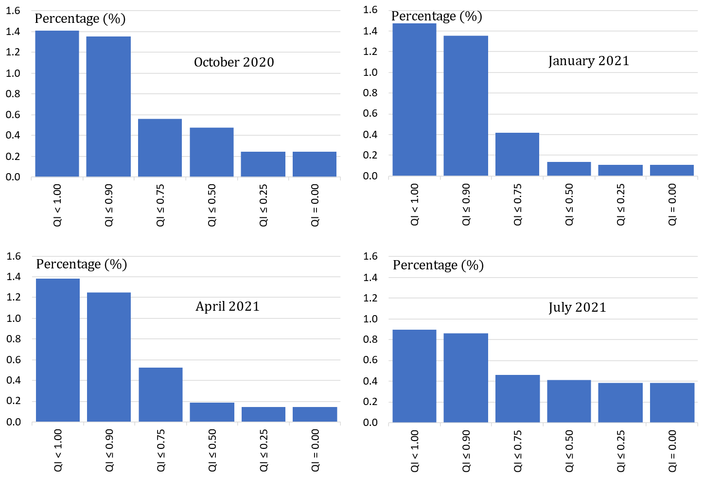
Figure 10 Percentage of rain gauge observations with a specified QI reduction after quality control. From the top: percentage contribution in each QI interval; cumulative percentage contribution (in %). From left: October 2020, January, April, and July 2021.

The graphs shown do not include the percentage contribution of measurements that were assigned a quality of 1.0; this is equal to about 98.5 %–99.1 %, which is much higher than the total contribution of all other values. In general, it can be seen from Fig. 10 that by far the greatest number of reductions in QI values was to values in the range (0.75, 0.90], and this is observed in all seasons of the year. Relatively large numbers of QI reductions to values in the range (0.50, 0.75] occur in winter (January) and spring (April), and relatively many data with quality reduced to a zero value occur in summer (July) and autumn (October).

The number of rain gauge observations with reduced quality is relatively small: below 1.5 %. For example, the contribution of data with QI reduced to zero (i.e. QI =0.0) ranges from about one-third to $\mathrm{1}/\mathrm{10}$ but grows to about one-half over the summer (July). In practice, this means that these data were rejected. Probably the most important reason is that in the summer convective precipitation often occurs, which is characterized by high intensities and strong spatial variability; moreover, rain gauges in no-rain situations react to morning dew condensation, which gives false rainfall measurements sometimes as high as 0.3 mm/10 min.

The most diverse distribution of QI reductions is observed in winter (January): most often there are small decreases in the QI value. In summer (July), this distribution is the least varied, which can be partially explained by the numerous QI reductions to zero.

5 Conclusions

1. Quality control of rain gauge data is essential, especially from the perspective of operational applications, when it is not possible to verify gauge data employing highly reliable precipitation measurements, such as manual Hellmann rain gauges, which are not available in real time.

2. It seems that the RainGaugeQC approach to the QC of rain gauge data, which consists of estimating the value of the QI of individual observations, enables more effective use of the data. On the one hand, it is a more cautious approach, as it does not eliminate all suspicious observations, and on the other hand, it enables flexible treatment of any suspected case of data incorrectness.

3. The IMGW rain station network consists mostly of rain stations equipped with two sensors: unheated and heated. This unique equipment allows the use of pairs of data to conduct much more effective QC. Comparing the observations from two sensors installed at the same location significantly increases the possibility of obtaining information about the uncertainty of measurements, for example by checking the time consistency of the data (TCC). This is especially important when measurements are carried out with tipping bucket rain gauges, which have relatively low reliability. The availability of observations from both sensors is especially important during the warm season, when convective phenomena prevail. The frequent lack of two sensors installed at the same location reduces the scheme's effectiveness to some extent; however, it remains at a satisfactory level.

4. It is worth considering the possibility of employing radar data in the RCC and SCC algorithms to detect erroneous rain gauge measurements and to assess their reliability based on the difference between the values from rain gauge and weather radar. The case study proved that the RainGaugeQC system can identify regionally inconsistent data thanks to the use of radar data as well as neighbouring rain gauge data.

5. The presented set of algorithms is based on empirical relationships that are strongly dependent on local conditions, both technical and geographic. The most important factors are the density of the rain station network, the availability of other data that can be used as a reference for QC (e.g. from the weather radar network), and the type of sensors (their failure rate and measurement uncertainty), as well as terrain orography, wind conditions, and surface precipitation type. Therefore, any changes in the network configuration necessitate recalibration of the algorithms.

6. The number of rain gauge observations with reduced QI following QC under the RainGaugeQC scheme is relatively small, as it is below 1.5 %. In all seasons, the highest number of QI value reductions was to values in the range [0.75, 0.90). The highest number of erroneous data (with QI reduced to zero) is found in summer (July) (approximately 0.4 %), whereas in other seasons it ranges from about 0.10 % to 0.23 %.

Appendix A: Detailed description of the radar conformity check (RCC) algorithm

RCC is performed to identify false zero precipitation and false gauge-reported precipitation measurement by applying radar data.

1. Identifying false zero precipitation

   Each gauge sensor value (G) less than 0.2 mm/10 min is checked against radar observations (R) at the gauge location and in its vicinity within a grid of 3 ×3 pixels.

   If at least one pixel of radar data had precipitation above 0.4 mm/10 min, then the gauge value measured by this sensor is assumed to be erroneous; thus, the sensor value is replaced by “no data” and the quality of this sensor is reduced to 0.

2. Identifying false gauge-reported precipitation

   Each gauge sensor value (G) above 0 mm/10 min is checked against radar observations (R) at the gauge location and in its vicinity within a grid of 3 ×3 pixels.

   If at least two radar pixels with QI >0.85 returned “no precipitation” (R=0 mm/10 min), then the following conditions are checked.

   • a.

     If for a given rain station, data are available only from one sensor (G) and G>0 mm/10 min, then the process proceeds as follows.

     • If the station is located in a mountain or foothill area, the sensor is considered erroneous – its value is replaced by G=0 mm and its quality reduced by 0.5.

     • If the station is located in a lowland area, the sensor is considered erroneous – its value is replaced by G=0 mm and its quality reduced by 0.25.

   • b.

     If for a given rain station, data are available from two sensors (heated G_h and unheated G_uh), G_h>0 mm/10 min, and G_uh>0 mm/10 min, then the process proceeds as follows.

     • If the station is located in a mountain or foothill area and values from both sensors are similar, i.e. SF (G_uh, G_h) is “true”, then the quality of both sensors is reduced by 0.75, but if SF (G_uh, G_h) is “false” then their qualities are reduced to QI =0 and the sensor values are replaced by “no data”.

     • If the station is located in a lowland area, then the sensor qualities are reduced to QI =0 and the sensor values are replaced by “no data”.

   • c.

     If for a given rain station, data are available from two sensors (heated G_h and unheated G_uh) and one of them reports “no precipitation” (i.e. G_h=0 mm/10 min or G_uh=0 mm/10 min), then the process proceeds as follows.

     • If the rain station is located in a mountain or foothill area and the values from both sensors are similar (i.e. SF (G_uh, G_h) is“true”), then the QI of the sensor which observed precipitation G>0 mm/10 min is reduced by 0.75, but if SF (G_uh, G_h) is “false”, then the QI of the sensor which reports G>0 mm/10 min is reduced to QI =0 and the sensor value is replaced by “no data”.

     • If the rain station is located in a lowland area, then the quality of the sensor that reports G>0 mm/10 min is reduced to QI =0 and the sensor value is replaced by “no data”.

Appendix B: Detailed description of the temporal conformity check (TCC) algorithm

The first step of this check is performed to detect constant values observed by a given sensor. If the same value (e.g. 0.1 mm/10 min) is reported for a certain number of time steps (e.g. nine consecutive observations), then the sensor is probably clogged. In this case, the blocked sensor has failed the TCC test, its QI is reduced to 0, and the TCC test cannot be performed for the other sensor.

The main part of TCC serves to identify rain stations for which there are large differences between values measured simultaneously by pairs of rain sensors (G_h, G_uh), which may be evidence of their low quality. This check requires measurements from both rain gauge sensors at the same location; it can thus be conducted only in the warm season, when both sensors provide measurements. This lasts from April to October, when data from unheated sensors (G_uh) are available; the heated sensors (G_h) operate all year round.

1. Pairs of simultaneous measurements from two sensors are verified for the last 12 time steps, excluding observations of poor quality (which means QI is 0.0 for previous time steps and for the current time step failed GEC, RC, or RCC check). If the number of pairs is high enough (at least nine), the cumulative sums are calculated.

   $$\begin{array}{}\text{(B1)}& S_{\mathrm{h}}={\sum }_{i=\mathrm{1}}^n{G}_{\mathrm{h},i},S_{\mathrm{uh}}={\sum }_{i=\mathrm{1}}^n{G}_{\mathrm{uh},i}\end{array}$$

2. The similarity of the accumulated sums is checked by means of the SF. If they differ significantly, i.e. if SF(S_h, S_uh) is “false”, then the data from both sensors have failed the TCC test and their quality is reduced by 0.25.

Appendix C: Detailed description of the spatial consistency check (SCC) algorithm

The SCC procedure consists of the following steps.

1. The Polish domain (900 km ×800 km) is divided into subdomains with dimensions of 100 km ×100 km. Only data with QI >0 after previous tests are subject to this check. It is optional (i) to analyse both sensors, heated and unheated, together or separately, as well as (ii) to also include data from the previous time step (10 min ago) if their QI =1.0. In order to perform this check there must be data available from at least three stations in a subdomain; otherwise, the test is not performed for that subdomain.

2. Based on data from rain stations (G) located in a given subdomain, the following percentiles are determined: 25 %, 50 % (median), and 75 % (Q₂₅(G), Q_med(G), and Q₇₅(G), respectively).

   The median absolute deviation (MAD) for a given subdomain is determined from the formula

   $$\begin{array}{}\text{(C1)}& \mathrm{MAD}={\displaystyle \frac{\mathrm{1}}{n}}{\sum }_{i=\mathrm{1}}^n\left|G_{\mathrm{i}}-Q_{\mathrm{med}}\left(G\right)\right|,\end{array}$$

   where n is the number of data, G_i is the ith sensor value, and Q_med(G) is the median.

3. The index D_i, which numerically determines the deviation of the precipitation value measured with the ith sensor from the median of all sensors within a given subdomain, is calculated from the formula (Kondragunta and Shrestha, 2006)

   $$\begin{array}{}\text{(C2)}& \begin{array}{rl}& D_i=\\ & \left\{\begin{array}{ll}\mathrm{0}& \mathrm{MAD}=\mathrm{0}\\ \frac{|G{}_i-Q_{\mathrm{med}}\left(G\right)|}{\mathrm{MAD}}& \mathrm{MAD}\ne \mathrm{0}\mathrm{and}{Q}_{\mathrm{75}}\left(G\right)=Q_{\mathrm{25}}\left(G\right)\\ \frac{|G{}_i-Q_{\mathrm{med}}\left(G\right)|}{Q_{\mathrm{75}}-Q_{\mathrm{25}}\left(G\right)}& \mathrm{MAD}\ne \mathrm{0}\mathrm{and}{Q}_{\mathrm{75}}\left(G\right)\ne Q_{\mathrm{25}}\left(G\right).\end{array}\right.\end{array}\end{array}$$

   Following calculation of the D_i values for all sensors within a given subdomain, three percentiles are determined: 90 %, 95 %, and 99 % (Q₉₀(D), Q₉₅(D), and Q₉₉(D), respectively).

4. If D_i≤Q₉₀(D), then the ith sensor is not an outlier and the test is passed.

   If this is not the case, the ith sensor is flagged and the formula in Eq. (C3) is applied to compare the index D_i with the three percentile values in order to determine to which class of outliers the given value belongs.

   $$\begin{array}{}\text{(C3)}& \mathrm{outlier}=\left\{\begin{array}{ll}\mathrm{strong}& D_i>Q_{\mathrm{99}}\left(D\right)\\ \mathrm{medium}& Q_{\mathrm{95}}\left(D\right)<D_i\le Q_{\mathrm{99}}\left(D\right)\\ \mathrm{weak}& Q_{\mathrm{90}}\left(D\right)<D_i\le Q_{\mathrm{95}}\left(D\right)\end{array}\right.\end{array}$$

   The procedure is repeated in four subdomains resulting from shifting the given subdomain vertically (west–east) and horizontally (south–north), i.e. in four directions, with offsets of 25 km (except for subdomains on the edges and corners of the domain, which are shifted in three and two directions, respectively). If the value measured with a given sensor is flagged in all analysed subdomains, it fails the SCC. If the values belonged to different classes of outliers, the weakest one is assigned to the sensor for further processing.

5. For sensors that failed the SCC, if the data from both sensors are available for a given rain station, if they are similar, i.e. SF(G_h, G_uh) is “true”, and if they passed the TCC, then the QI for the sensor is not reduced.

   Otherwise, each outlier is verified against radar data. For this purpose the following values are determined within a grid of 5 ×5 pixels around this rain station location: min(QI(R)) – the minimum quality QI of the radar precipitation R; $R_{\max }=\max \left(R\text{:}\mathrm{QI}\left(R\right)>\mathrm{0.75}\right)$ – the maximum value of radar precipitation with a quality above 0.75; QI(R_max) – the quality of the maximum value of radar precipitation R_max. This verification algorithm is as follows.

   $$\begin{array}{}\text{(C4)}& \begin{array}{rl}& \mathrm{If}\min \left(\mathrm{QI}\left(R\right)\right)>\mathrm{0.75},\mathrm{then}\text{:}\mathrm{if}{R}_{\max }=\mathrm{0},\mathrm{then}\mathrm{the}\\ & \mathrm{quality}\mathrm{is}\mathrm{reduced}\mathrm{by}\mathrm{1.0}\mathrm{and}G=\mathrm{`}\mathrm{`}\mathrm{no}\mathrm{data}\text{”};\\ & \mathrm{if}\left(G>\mathrm{1.0}\mathrm{mm}\right)\mathrm{and}\\ & \left({\displaystyle \frac{G}{R_{\max }}}<{\displaystyle \frac{\mathrm{QI}\left(R_{\max }\right)}{\mathrm{4.0}}}\mathrm{or}{\displaystyle \frac{G}{R_{\max }}}>{\displaystyle \frac{\mathrm{4.0}}{\mathrm{QI}\left(R_{\max }\right)}}\right),\mathrm{then}\text{:}\\ & \mathrm{QI}=\left\{\begin{array}{ll}\mathrm{QI}-\mathrm{1.00}& \mathrm{strong}\mathrm{outlier}\\ \mathrm{QI}-\mathrm{0.50}& \mathrm{medium}\mathrm{outlier}\\ \mathrm{QI}-\mathrm{0.20}& \mathrm{weak}\mathrm{outlier}\end{array}\right.\\ & \mathrm{if}\left(G>\mathrm{1.0}\mathrm{mm}\right)\mathrm{and}\left({\displaystyle \frac{G}{R_{\max }}}\ge {\displaystyle \frac{\mathrm{QI}\left(R_{\max }\right)}{\mathrm{4.0}}}\mathrm{and}\right.\\ & \left.{\displaystyle \frac{G}{R_{\max }}}\le {\displaystyle \frac{\mathrm{4.0}}{\mathrm{QI}\left(R_{\max }\right)}}\right),\mathrm{then}\text{:}\\ & \mathrm{QI}=\left\{\begin{array}{ll}\mathrm{QI}-\mathrm{0.25}& \mathrm{strong}\mathrm{outlier}\\ \mathrm{QI}-\mathrm{0.10}& \mathrm{medium}\mathrm{outlier}\\ \mathrm{QI}& \mathrm{weak}\mathrm{outlier}\end{array}\right.\\ & \mathrm{if}\left(G\le \mathrm{1.0}\mathrm{mm}\right)\mathrm{or}\left(\min \left(\mathrm{QI}\left(R\right)\right)\le \mathrm{0.75}\right),\mathrm{then}\text{:}\\ & \mathrm{QI}=\left\{\begin{array}{ll}\mathrm{QI}-\mathrm{0.25}& \mathrm{strong}\mathrm{outlier}\\ \mathrm{QI}-\mathrm{0.10}& \mathrm{medium}\mathrm{outlier}\\ \mathrm{QI}& \mathrm{weak}\mathrm{outlier}\end{array}\right.\end{array}\end{array}$$

   Here, $\frac{\mathrm{4.0}}{\mathrm{QI}\left(R_{\max }\right)}$ is the limitation to the magnitude of disparity $\frac{G}{R_{\max }}$ determined empirically.

An alternative simplified analysis of the spatial consistency of rain gauge data may be performed analogously to steps 1–4, especially if radar data are unavailable. In this case, it is sufficient to determine only the Q₉₅(D) percentile. Here, if in all subdomains D_i>Q₉₅(D), the sensor fails the SCC, and the QI is decreased by 0.10.