Information content and aerosol property retrieval potential for different types of in situ polar nephelometer data

Polar nephelometers are in situ instruments used to measure the angular distribution of light scattered by aerosol particles. These types of measurements contain substantial information about the properties of the aerosol being probed (e.g. concentrations, sizes, refractive indices, shape parameters), which can be retrieved through inversion algorithms. The aerosol property retrieval potential (i.e. information content) of a given set of measurements depends on the spectral, polarimetric, and angular characteristics of the polar nephelometer that was used to acquire the measurements. To explore this issue quantitatively, we applied Bayesian information content analysis and calculated the metric degrees of freedom for signal (DOFS) for a range of simulated polar nephelometer instrument configurations, aerosol models and test cases, and assumed levels of prior knowledge about the variances of specific aerosol properties. Assuming a low level of prior knowledge consistent with an unconstrained ambient/field measurement setting, we demonstrate that even very basic polar nephelometers (single wavelength, no polarization capability) will provide informative measurements with a very high retrieval potential for the size distribution and refractive index state parameters describing simple unimodal, spherical test aerosols. As expected, assuming a higher level of prior knowledge consistent with well-constrained laboratory applications leads to a reduction in potential for information gain via performing the polarimetric measurement. Nevertheless, we show that in this situation polar nephelometers can still provide informative measurements: e.g. it can be possible to retrieve the imaginary part of the refractive index with high accuracy if the laboratory setting makes it possible to keep the probed aerosol sample simple. The analysis based on a high level of prior knowledge also allows us to better assess the impact of different polar nephelometer instrument design features in a consistent manner for retrieved aerosol parameters. The results indicate that the addition of multi-wavelength and/or polarimetric measurement capabilities always leads to an increase in information content, although in some cases the increase is negligible, e.g. when adding a fourth, near-IR measurement wavelength for the retrieval of unimodal size distribution parameters or if the added polarization component has high measurement uncertainty. By considering a more complex bimodal, non-spherical-aerosol model, we demonstrate that performing more comprehensive spectral and/or polarimetric measurements leads to very large benefits in terms of the achieved information content. We also investigated the impact of angular truncation (i.e. the loss of measurement information at certain scattering angles) on information content. Truncation at extreme angles (i.e. in the near-forward or near-backward directions) results in substantial decreases in information content for coarse-aerosol test cases. However for fine-aerosol test cases, the sensitivity of DOFS to extreme-angle truncation is noticeably smaller and can be further reduced by performing more comprehensive measurements. Side angle truncation has very little effect on information content for both the fine and coarse test cases. Furthermore, we demonstrate that increasing the number of angular measurements generally increases the information content. However, above a certain number of angular measurements (∼20–40) the observed increases in DOFS plateau out. Finally, we demonstrate that the specific placement of angular measurements within a nephelometer can have a large impact on information content. As a proof of concept, we show that a reductive greedy algorithm based on the DOFS metric can be used to find optimal angular configurations for given target aerosols and applications.

1 Introduction

Aerosols are condensed-phase particles suspended in the air that are distributed ubiquitously in the atmosphere. Aerosol particles have a broad range of sizes spanning orders of magnitudes, and they possess diverse physical and chemical properties. They affect the global climate either by directly scattering or absorbing solar radiation or by influencing cloud formation processes (Boucher et al., 2013). Aerosol particles are also one of the major components of air pollution and aerosol exposure has been linked to cardiovascular and pulmonary diseases and premature deaths (Cohen et al., 2017; Lelieveld et al., 2015).

Due to the importance of aerosol particles for the global atmospheric system and for public health, a multitude of methods have been developed to measure and characterize these particles with both in situ and remote-sensing instruments. Remote-sensing methods rely on the interaction of aerosols with solar radiation or laser light and typically involve detection of the elastically scattered light. In particular, many instruments have been designed to measure the angular dependence of scattered radiance (radiometry), with optional measurement of its dependence on polarization state (polarimetry). Radiometry and polarimetry are the cornerstones of ground-based and space-borne remote-sensing applications because the resulting measurements contain retrievable information on aerosol microphysical properties, which can be obtained via inversion algorithms. Well-known examples of space-borne remote-sensing instruments include the Moderate Resolution Imaging Spectrometer (MODIS; King et al., 1992), the Multi-angle Imaging SpectroRadiometer (MISR; Lee et al., 2009), and the Polarization and Directionality of Earth's Reflectance (POLDER; Deuzé et al., 2001) instrument. In terms of ground-based polarimetric observations, the prime example is the AEosol RObotic NETwork (AERONET; Holben et al., 1998), which is a coordinated network of sun photometers at more than 600 sites worldwide.

Three design aspects are fundamentally important for aerosol polarimetry instruments: (i) the spectral coverage, i.e. the number of wavelengths at which light scattering is measured, (ii) the polarization measurement capability, and (iii) the number and position of the probed angles. Over the last few decades, technological advancements have led to substantial instrumentation improvements in terms of all three of these design aspects (Dubovik et al., 2019). Parallel to these instrumentation developments, advanced aerosol property retrieval algorithms have been designed to better utilize these more informative polarimetric measurements. For example, GRASP-OPEN (Generalized Retrieval of Aerosol and Surface Properties) is a well-established retrieval algorithm that was designed to take advantage of enhanced polarimetric measurements in order to improve the scope and accuracy of aerosol property retrievals (Dubovik et al., 2011, 2014, 2021).

Polar nephelometers, which are in situ instruments for radiometric and polarimetric aerosol measurements, have a rich history dating back to the 1940s (Waldram, 1945). The main physical quantity measured by polar nephelometers is the phase function (denoted here as PF), which is a measure of angular distribution of scattered light radiance by aerosol particles given non-polarized incident light. A subclass of polar nephelometers are also capable of measuring the polarized phase function (denoted here as PPF), which is the angular distribution of the portion of linearly polarized scattered light given non-polarized incident light. Note that some polar nephelometers are capable of measuring more scattering quantities (e.g. Hu et al., 2021), but in this study we only focus on instruments that measure PF and PPF.

A variety of polar nephelometer designs has been introduced over the years. The first design class of these instruments is the goniometer-type polar nephelometer, which measures angularly resolved light scattering using a rotating detector (e.g. Waldram, 1945). The major disadvantage of these types of instruments is the long sampling time required to measure a full phase function, which severely limits their usability in field applications. A second design class is the multi-detector-type instrument, which enables more rapid measurements by employing detectors at fixed positions to probe PF or PPF at discreet angles simultaneously. Multi-detector nephelometers can have either very basic designs (e.g. four angles and only one wavelength; Li et al., 2019), or more complex designs, such as the instruments introduced by Barkey et al. (2007) and Nakagawa et al. (2016), which measure both PF and PPF at 21 and 17 angles, respectively. A third design class is the laser imaging nephelometer (Dolgos and Martins, 2014; Ahern et al., 2022). The laser imaging nephelometer illuminates aerosol particles using laser light and collects the scattered light on a charged coupled device (CCD). The angularly resolved scattering measurements are then extracted from the image collected by the CCD. An example of a laser imaging nephelometer is the Polarized Imaging Nephelometer introduced by Dolgos and Martins (2014), which measures PF and PPF over 174 angles and at three different wavelengths.

The angularly resolved measurements provided by polar nephelometers enable the retrieval of a large number of aerosol properties via inversion algorithms such as GRASP-OPEN (which can be applied in a versatile manner to both remote-sensing and in situ measurement data: Espinosa et al., 2019; Dubovik et al., 2014, 2021). Furthermore, since these instruments provide measurements that are in principle quite similar to remote-sensing data, they can be used as well-constrained test beds for evaluation and improvement of the inversion algorithms used by the remote-sensing community (Schuster et al., 2019). However, the high dimensionality of polar nephelometer measurements with respect to spectral, polarimetric, and multi-angle measurement options also presents an instrument design challenge. In particular, it raises the following questions. (i) Which types of measurements should be prioritized and optimized in order to maximize the information content concerning the underlying aerosol properties? (ii) Can relatively non-informative measurement types be identified in order to prevent overdesign and complexities that could hamper robustness or cost-effectiveness?

Bayesian information content analysis is a tool that has been used extensively by the remote-sensing community to guide such instrument design challenges by enabling the calculation of quantitative information content metrics for specific instrumentation configurations, settings, and applications (Rodgers, 2000). For example, the framework has been used to demonstrate the importance of polarized and multi-angle scattering measurements in the context of space-borne satellite measurements and ground-based sun photometers (Knobelspiesse and Nag, 2018; Chen et al., 2017; Ding et al., 2016; Xu and Wang, 2015; Ottaviani et al., 2013; Knobelspiesse et al., 2012). However, to the best of our knowledge, the framework has not yet been applied to in situ light scattering measurements in order to tackle the design challenges posed above. As well as being used to assess information content, the Bayesian theoretical framework (Rodgers, 2000) can also be used as an inversion method. In this context, the Bayesian approach can be regarded as a particular case of the more general retrieval method employed in GRASP-OPEN, as discussed by Dubovik et al. (2021), where it is also noted that Bayesian-based retrievals can be hampered by the requirement of directly specifying a priori constraints for all aerosol state parameters.

In this study, we use a Bayesian framework purely as a method for assessing the information content of synthetic measurement data in order to investigate the challenges associated with polar nephelometer instrument design. Specifically, we assess and compare the aerosol property retrieval potential of different polar nephelometer instrument configurations given different target applications and assumed prior knowledge. Furthermore, within the theoretical framework, we use a case study to demonstrate how a well-known optimization algorithm (a reductive greedy algorithm) can be used to determine the optimal placements of the angular sensors in a polar nephelometer.

The paper is structured in the following manner. In Sect. 2, we provide general information on the Bayesian information content framework, while in Sect. 3 we introduce the specific methodological aspects used to construct the information content analysis used in this study. In Sect. 4 we present the results of the analysis, including an overview of the information content of different polar nephelometer instrument designs, an assessment of the value of spectral and polarimetric measurements, an investigation of measurement artefacts associated with scattered light truncation, and the results of the angular sensor placement optimization case study. Finally, we summarize the conclusions of the study in Sect. 5.

2 Theory: information content analysis and degrees of freedom for signal (DOFS)

In scientific and engineering applications it is typically not possible to measure quantities of interest directly. Instead, the values of such quantities must be inferred indirectly from measurements of causally related intermediary quantities. These types of inference problems are known generically as inverse problems. Inverse problems can be expressed mathematically by considering a so-called state vector, x, which contains the N desired parameters to be retrieved (i.e. the state parameters x_i), and an observation vector, y, which corresponds to a set of M measurements conducted by an instrument. The vectors x and y are assumed to be related to each other through the following equation:

$$\begin{array}{}\text{(1)}& \mathit{y}=F\left(\mathit{x}\right)+\mathit{\epsilon },\end{array}$$

where F (x) is referred to as the forward model. The forward model maps the state vector into measurement space based on the underlying physical processes that are involved. For example, the Mie solution to Maxwell's equations is a forward model that relates the microphysical properties of spherical particles x (e.g. size, refractive index) to measurable optical parameters y (e.g. PF and PPF). The ε vector in Eq. (1) represents the error originating from measurement noise as well as the error resulting from the limitations of a particular forward model.

The main objective in an inverse problem is to retrieve a best estimate of the state vector ($\widehat{\mathit{x}})$ given a measurement vector y and the relationship in Eq. (1). This can be achieved in a number of different ways. In inverse problems related to atmospheric observations, some prior knowledge of the state parameters to be retrieved is typically available. In such cases, Bayesian inference (Rodgers, 2000) is a well-established method for the retrieval of state vectors. For a forward model that describes the underlying physics of the problem and that can be locally linearized in the state space, a measurement vector y corresponding to a reference state vector, x₀, can be written as

$$\begin{array}{}\text{(2)}& \mathit{y}=\mathbf{K}{\mathit{x}}_{\mathrm{0}}+\mathit{\epsilon },\end{array}$$

where K is the Jacobian matrix of the forward model at the reference point x₀ (i.e. K = ${\left.\frac{\partial F\left(\mathit{x}\right)}{\partial \mathit{x}}\right|}_{x=x_{\mathrm{0}}})$, which has dimensions of [M×N]. Under the assumptions of normally distributed measurement errors and a priori state parameter ranges, the Bayes theorem can be applied to infer an estimated state vector, $\widehat{\mathit{x}}$, from the measurement vector y. Using the Bayes theorem, $\widehat{\mathit{x}}$ and its corresponding error covariance matrix $\widehat{\mathbf{S}}$ then become

$$\begin{array}{}\text{(3)}& {\displaystyle }\widehat{x}=\widehat{\mathbf{S}}{\mathbf{K}}^{\mathrm{T}}{\mathbf{S}}_{\mathit{\epsilon }}^{-\mathrm{1}}(\mathbf{K}{\mathit{x}}_{\mathrm{0}}+\mathit{\epsilon })+\left(\mathbf{I}-\widehat{\mathbf{S}}{\mathbf{K}}^{\mathrm{T}}{\mathbf{S}}_{\mathit{\epsilon }}^{-\mathrm{1}}\mathbf{K}\right){\mathit{x}}_{\mathrm{a}},\text{(4)}& {\displaystyle }{\widehat{\mathbf{S}}}^{-\mathrm{1}}={\mathbf{K}}^{\mathrm{T}}{\mathbf{S}}_{\mathit{ϵ}}^{-\mathrm{1}}\mathbf{K}+{\mathbf{S}}_{\mathrm{a}}^{-\mathrm{1}}.\end{array}$$

Detailed descriptions on how to derive these formulae are provided in Sect. 2 of Rodgers (2000). The matrix S_ε is the measurement error covariance matrix. The diagonal elements of S_ε represent the measurement uncertainties for each of the measured elements y_i, while the off-diagonal elements describe the covariance between the errors for different elements. The vector x_a is the a priori vector in the state space, which contains what one believes to be the expected values for the state vector prior to the measurement being performed (i.e. the prior knowledge of the state space variables). The matrix S_a is the a priori covariance matrix which describes the expected spread of the state vector parameters in the state space. The matrix $\widehat{\mathbf{S}}$ is the retrieval (posterior) error covariance matrix, which describes the spread of the estimated state vector $\widehat{\mathit{x}}$. The square root of diagonal elements of $\widehat{\mathbf{S}}$ corresponds to the retrieval (posterior) uncertainties in individual state parameters, and in this study they are denoted as σ_post,i for the given parameters x_i.

By defining $\widehat{\mathbf{S}}{\mathbf{K}}^{\mathrm{T}}{\mathbf{S}}_{\mathit{\epsilon }}^{-\mathrm{1}}\mathbf{K}$ as the so-called averaging kernel matrix A, Eq. (3) can be rewritten as

$$\begin{array}{}\text{(5)}& \widehat{\mathit{x}}={\mathbf{Ax}}_{\mathrm{0}}+\left(\mathbf{I}-\mathbf{A}\right){\mathbf{x}}_{\mathbf{a}}+{\mathit{\epsilon }}_{\mathbf{x}},\end{array}$$

where I is the identity matrix and ε_x is the retrieval error, which corresponds to the transformation of measurement error from the measurement space to the state space. The averaging kernel matrix A captures the sensitivity of the retrieved state vector $\widehat{\mathit{x}}$ to the reference state vector x₀. The diagonal elements of A (A_ii) are referred to as the degrees of freedom for signal (DOFS_i) for the given state parameters x_i. These elements can take values between 0 and 1. As shown in Eq. (5), the DOFS_i values can be interpreted as the normalized factors used to compute the optimal estimate retrieval result (and retrieval error) as a weighted average of the transformed measurement errors and the a priori parameter ranges following the Bayes theorem. That is, the DOFS_i are quantitative metrics that describe the information content of a given measurement in relation to prior knowledge. For example, a DOFS_i value close to 1 indicates that a particular measurement makes a greater contribution to the retrieval of a given state parameter ${\widehat{x}}_i$ compared to what is known a priori about the value of that state parameter (i.e. DOFS_i→1 indicates a more informative measurement). On the other hand, a DOFS_i value closer to 0 indicates that a priori knowledge makes the dominant contribution to the retrieval of a state parameter ${\widehat{x}}_i$, whereas the corresponding measurement only has little influence (i.e. the measurement is non-informative).

To quantify the overall information content of a measurement, the total DOFS for all retrievable state parameters is defined according to the following sum:

$$\begin{array}{}\text{(6)}& \mathrm{DOFS}=\mathrm{trace}\left(\mathbf{A}\right)={\sum }_{i=\mathrm{1}}^{\mathrm{N}}{A}_{ii}.\end{array}$$

Therefore, DOFS assumes values between 0 and N. This means that for a hypothetically perfect measurement DOFS = N, the number of state parameters considered in the forward model. Dividing DOFS by N provides the normalized DOFS, which we denote as nDOFS.

It must be stressed that DOFS values depend intrinsically on the assumed a priori variables and measurement uncertainties when applying Bayesian inference. Therefore, one must be careful not to overinterpret absolute DOFS values without considering their full context. These issues can be partially avoided by using DOFS values in a relative manner, e.g. by ranking different designs with respect to achievable information content. As an alternative approach to circumventing the influence of assumed prior knowledge, Alexandrov and Mishchenko (2017) proposed the use of S_pro as an information content metric, given by

$$\begin{array}{}\text{(7)}& {\mathbf{S}}_{\mathrm{pro}}=({\mathbf{K}}^{\mathrm{T}}{\mathbf{S}}_{\mathit{ϵ}}^{-\mathrm{1}}\mathbf{K}{)}^{-\mathrm{1}}.\end{array}$$

Mathematically, S_pro represents the error covariance matrix of a state vector retrieved from a measurement using least squares minimization (LSM) without considering a priori knowledge. The diagonal elements of S_pro, denoted as ${\mathit{\sigma }}_{\mathrm{pro}}^{\mathrm{2}}$, represent the variance of the LSM-retrieved state parameters. In this study, we use S_pro as an additional information content metric to support our discussion of DOFS values. A summary of all the information content metrics used in this study is provided in Table 1. Further details about Bayesian inference and DOFS can be found in numerous previous studies (Knobelspiesse and Nag, 2018; Ding et al., 2016; Xu and Wang, 2015; Hasekamp and Landgraf, 2005).

Table 1 Summary of the information content metrics used in this study.

3 Implementation of information content analysis into in situ polar nephelometer data

In this study, the Bayesian framework described in Sect. 2 was used to investigate the information content and aerosol property retrieval potential of different polar nephelometer measurement configurations. Figure 1 summarizes the implementation of this analysis, while the subsequent subsections explain inputs, calculation steps, and outputs in more detail.

Non-linearity of light scattering as a function of aerosol state parameters is a central aspect of the inverse problem of aerosol polarimetry. One effect is that the information content of a polarimetric measurement also depends on the properties of the aerosol under investigation (besides dependence on instrument features and a priori knowledge of the properties of the aerosol sample). Therefore, our general approach is to investigate different aerosol test cases, e.g. fine- versus coarse-mode aerosol or non-absorbing versus absorbing aerosol.

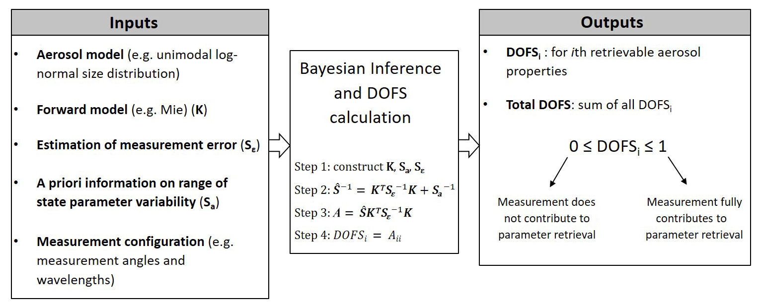
Figure 1 A schematic overview of the implementation of the Bayesian information content analysis.

3.1 Measurement configurations

The measurement capabilities of polar nephelometers differ in three main aspects: the spectral characteristics (i.e. the number of measurement wavelengths N_λ), radiometric-only or polarimetric measurement (PF or PF and PPF, respectively), and the angular characteristics (i.e. the number and position of probed angles N_θ). The measurement space vector for a particular instrument will have dimensions of either N_λ×N_θ or $\mathrm{2}\times N_{\mathit{\lambda }}\times N_{\mathit{\theta }}$ for radiometric or polarimetric instruments, respectively. That is, we assume that the angular and spectral dimensions are equivalent for PF and PPF. In this study, we examined a variety of polar nephelometer configurations that differ according to the above design features.

The general angular geometry of the problem is shown in Fig. 2. The polar scattering angle (θ) range over which discrete light scattering measurements are performed ranges from θ=0^∘ (forward direction relative to the direction of the incident light) to θ=180^∘ (backward-scattered light).

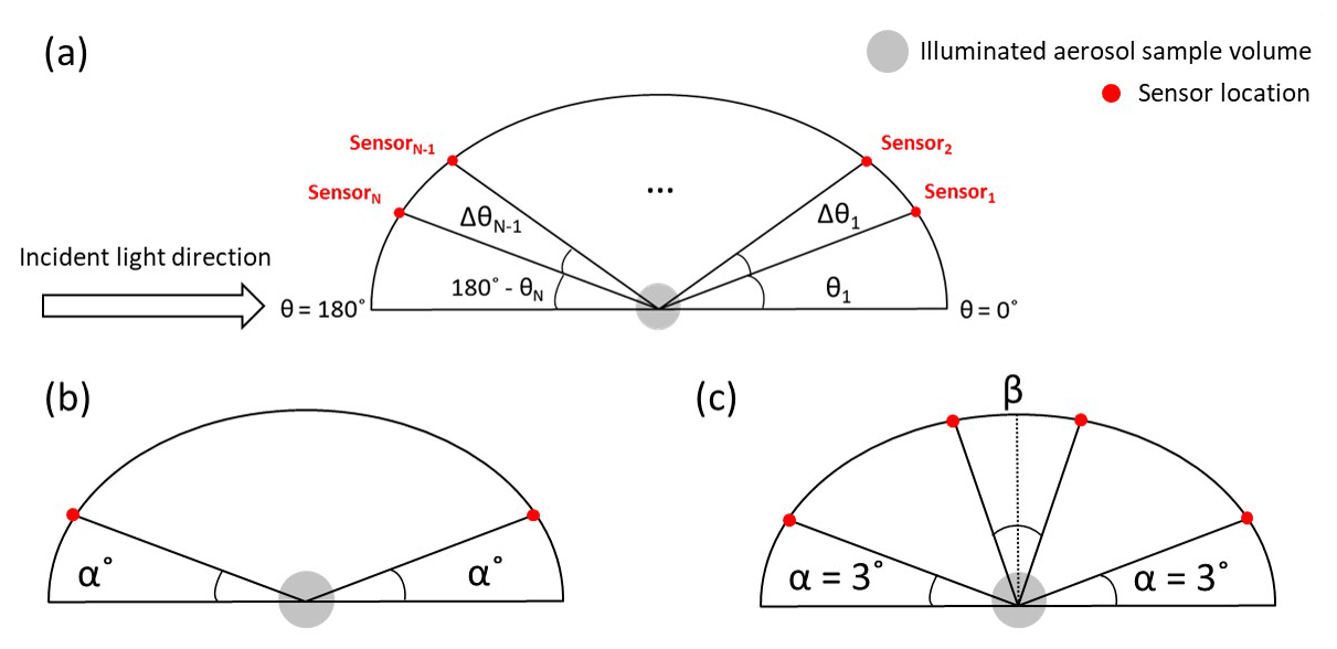
Figure 2 Schemes of scattering measurement geometry: (a) polar angles of sensors, (b) truncation around extreme angles, and (c) truncation around right angle.

3.1.1 Angular characteristics: extreme truncation angles

Probing scattering angles very close to the incident light beam is a general problem in all types of nephelometers (Moosmüller and Arnott, 2003) due to, e.g., blockage of this beam or interference between the incident and scattered light. This leads to truncation of the probed angle range at extreme values representing the forward and backward directions. The difference between the smallest measurable scattering angle θ₁ and 0^∘ is referred to as the forward truncation angle and is shown as α in Fig. 2b. The difference between the largest measurable scattering angle θ_N and 180^∘ is referred to as the backward truncation angle and is also represented as α in Fig. 2b. That is, we assume that the forward and backward truncation angles are equal in our simulations, since these two angles are similar in many nephelometers (e.g. Bian et al., 2017; Nakagawa et al., 2016; Manfred et al., 2018). To study the effect the extreme-angle truncation, we varied α over the set of values [0, 1, 3, 5, 10, 20, 40^∘], while keeping Δθ_i constant at 1^∘ (a typical value for laser imaging polar nephelometers; Dolgos and Martins, 2014).

3.1.2 Angular characteristics: side truncation angles

We are currently testing and validating a laser imaging nephelometer similar in design to the instrument by Dolgos and Martins (2014), which suffers from a gap in measurements near 90^∘ scattering angles. Here, we refer to this type of measurement gap as side angle truncation. To investigate side angle truncation we assume that it is symmetric around 90^∘ and represent it by a single angle β, which represents the angle between the closest sensors to 90^∘ in both the forward and backward scattering regions as shown in Fig. 2c. We varied β over the set of values [1, 11, 21, 31, 41, 51, 61, 71, 81, 91^∘] while keeping Δθ=1^∘ and α=3^∘.

3.1.3 Angular characteristics: number of probed angles assuming evenly distributed measurements

For an instrument covering N_θ distinct angles, each data point has an associated angle θ_i. The angular difference between two adjacent data points, hereafter referred to as sensors, is defined as $\mathrm{\Delta }{\mathit{\theta }}_i:={\mathit{\theta }}_i-{\mathit{\theta }}_{i-\mathrm{1}}$. As a default setup, we assumed that all sensors are evenly distributed (i.e. Δθ_i=Δθ). To investigate the effect of sensor number on the information content, we varied Δθ over a range that encompasses the sensor numbers of instruments previously reported in the literature. Examples at either end are the instrument described by Li et al. (2019) with four sensors and laser imaging polar nephelometers with a maximal angular resolution of Δθ≈1^∘ (Dolgos and Martins, 2014). The range of simulated Δθ values is shown in Table 2, along with the corresponding N_θ values for base case truncation angles, i.e. α=5^∘ and β=0^∘. In all cases we assume that the angular field of view of each sensor is infinitesimally small (i.e. that there is negligible overlap between adjacent sensors). This simplification has little effect on resulting information content as long as the angular field of view of the sensors is small (e.g. ∼1^∘) and less than the angular separation between adjacent sensors, whereas the results do not apply if the sensors have a wide field of view. In laser-imaging-type nephelometers, the maximal number of informative angular measurements is typically limited by the effective field of view of the pixels rather than the angular separation between adjacent pixels.

Table 2 Simulated Δθ values and corresponding number of probed angles for a configuration with evenly distributed sensors and α=5^∘ truncation in forward and backward directions.

3.1.4 Spectral measurement capabilities

We considered three different spectral measurement settings:

1. single-wavelength measurement at 532 nm (1λ)

2. three-wavelength measurement at 450, 532, and 630 nm (3λ)

3. four-wavelength measurement at 450, 532, 630, and 1020 nm (4λ).

The selected visible wavelengths, i.e. 450, 532, and 630 nm, are chosen to resemble the wavelengths of our custom-built laser imaging polar nephelometer that is currently being developed. An NIR wavelength measurement is typically not included in existing polar nephelometer designs. However, measurements at λ=1020 nm are performed extensively by ground-based passive remote-sensing instruments (e.g. within AERONET), and they are thought to benefit the retrieval of coarse-mode particle properties. Therefore, we used 4λ as a test case to investigate the potential benefits of including an NIR measurement in an in situ instrument.

3.2 Assumptions on measurement error covariance matrix (S_ε)

The measurement error covariance matrix, S_ε (Eq. 3), represents the uncertainty in the measurements of specific parameters (diagonal matrix elements) as well as the covariance of measurement errors between different data points (non-diagonal elements). For all the analyses we assume normally distributed random measurement errors.

For PF and PPF at any given wavelength, we chose measurement errors based on those reported by Dolgos and Martins (2014) for their laser imaging polar nephelometer. Specifically, we took the average values of the errors reported by these authors for aerosols with high and low scattering coefficient cases. That is,

$$\begin{array}{}\text{(8)}& {\displaystyle }& {\displaystyle }{\mathit{\sigma }}_{\mathrm{meas},\mathrm{PF}}({\mathit{\theta }}_j,{\mathit{\lambda }}_i)=\mathrm{0.046}\times \mathrm{PF}({\mathit{\theta }}_j,{\mathit{\lambda }}_i),\text{(9)}& {\displaystyle }& {\displaystyle }{\mathit{\sigma }}_{\mathrm{meas},\mathrm{PPF}}({\mathit{\theta }}_j,{\mathit{\lambda }}_i)=\mathrm{0.056}.\end{array}$$

The uncertainties described in Eqs. (8) and (9) represent the square root of the diagonal elements of S_ε (λ_i). Although it is quite common in the related information content literature to assume that there is no covariance of errors in measurements at different angles (Knobelspiesse and Nag, 2018; Chen et al., 2017; Xu and Wang, 2015), it is feasible that certain instrumentation or data processing biases influence adjacent angular measurements in a causally connected manner, thus resulting in covariant errors. To construct a more realistic covariance matrix, Knobelspiesse et al. (2012) used a Markov process to assign off-diagonal element values in the covariance matrix. In our analysis, we used a similar approach to account for covariance between adjacent angular measurements if the measurements are of the same type and from equal wavelengths. Furthermore, it was assumed that no error covariance exists between measurement of different types (PF, PPF) and/or different wavelengths. We employed Eq. (10a, c) to construct the error covariance matrix of a given measurement type at a given wavelength.

$$\begin{array}{}\text{(10a)}& {\displaystyle }{S}_{\mathit{\epsilon },i,j}={\mathit{\sigma }}_i^{\mathrm{2}}\mathrm{if}i=j\text{(10b)}& {\displaystyle }\begin{array}{r}{S}_{\mathit{\epsilon },i,j}={\mathit{\sigma }}_i{\mathit{\sigma }}_j{\mathit{\rho }}^{\mathrm{|}{\mathit{\theta }}_i-{\mathit{\theta }}_j\mathrm{|}}\mathrm{if}i\ne j(\mathrm{for}\mathrm{same}\mathrm{measurement}\\ \mathrm{types}\mathrm{and}\mathrm{wavelength})\end{array}\text{(10c)}& {\displaystyle }{S}_{\mathit{\epsilon },i,j}=\mathrm{0}\mathrm{Otherwise}\end{array}$$

We set ρ=0.7, for which ${\mathit{\rho }}^{\mathrm{|}{\mathit{\theta }}_i-{\mathit{\theta }}_j\mathrm{|}}$ varies from 0.7 at ${\mathit{\theta }}_i-{\mathit{\theta }}_j=\mathrm{1}$^∘ to below 0.05 at ${\mathit{\theta }}_i-{\mathit{\theta }}_j=\mathrm{10}$^∘, allowing for moderate covariance between adjacent angular measurements.

In the general case of a multi-wavelength configuration (with N_λ wavelength measurements) and for both PF and PPF measurements, the total covariance matrix will look like the block matrix demonstrated in Eq. (11), where each diagonal matrix block corresponds to the individual covariance matrices for a given type of measurement (PF or PPF) at a specific wavelength. For S_ε, the dimension value of N_tot is N_λ×N_θ and $\mathrm{2}\times N_{\mathit{\lambda }}\times N_{\mathit{\theta }}$ for radiometric and polarimetric instruments, respectively.

$${\mathbf{S}}_{\mathit{\epsilon }}=\left[\begin{array}{cc}\begin{array}{ccc}{\mathbf{S}}_{\mathit{\epsilon },\mathbf{PF}}\left({\mathit{\lambda }}_{\mathrm{1}}\right)& \mathrm{\dots }& \mathbf{0}\\ \mathrm{⋮}& \mathrm{\ddots }& \mathrm{⋮}\\ \mathbf{0}& \mathrm{\dots }& {\mathbf{S}}_{\mathit{\epsilon },\mathbf{PF}}\left({\mathit{\lambda }}_{N_{\mathit{\lambda }}}\right)\end{array}& \mathbf{0}\end{array}\right.$$

$$\begin{array}{}\text{(11)}& {\left.\begin{array}{cc}\mathbf{0}& \begin{array}{ccc}{\mathbf{S}}_{\mathit{\epsilon },\mathbf{PPF}}\left({\mathit{\lambda }}_{\mathrm{1}}\right)& \mathrm{\dots }& \mathbf{0}\\ \mathrm{⋮}& \mathrm{\ddots }& \mathrm{⋮}\\ \mathbf{0}& \mathrm{\dots }& {\mathbf{S}}_{\mathit{\epsilon },\mathbf{PPF}}\left({\mathit{\lambda }}_{N_{\mathit{\lambda }}}\right)\end{array}\end{array}\right]}_{N_{\mathrm{tot}}\times N_{\mathrm{tot}}}\end{array}$$

3.3 Aerosol model, state parameters, and test cases

3.3.1 Aerosol model and corresponding state parameters

As an aerosol model, we generally considered aerosol particles to be homogeneous spheres with log-normally distributed size distribution modes and uniform composition within each size mode (however, a small number of simulations are also performed for non-spherical particles, as explained below). The assumption of log-normally distributed size modes is very typical in aerosol science (Seinfeld and Pandis, 2006). Furthermore, it is common to employ multi-modal log-normal functions to construct volumetric particle size distributions for a complete aerosol. This is the method adopted in this study, where Eq. (12) describes the general equation we used for a multi-modal log-normal volume particle size distribution (VPSD).

$$\begin{array}{}\text{(12)}& \begin{array}{rl}& {\displaystyle \frac{\mathrm{d}V}{\mathrm{dln}\left(r\right)}}=\sum _{i=\mathrm{1}}^{N_{\mathrm{mode}}}{\displaystyle \frac{V_i}{\sqrt{\mathrm{2}\mathit{\pi }}\ln \left({\mathrm{GSD}}_i\right)}}\exp \\ & \left[{\displaystyle \frac{-{\left(\ln \left(r\right)-\ln \left({\mathrm{VMR}}_i\right)\right)}^{\mathrm{2}}}{\mathrm{2}\left(\ln \right({\mathrm{GSD}}_i){)}^{\mathrm{2}}}}\right]\end{array}\end{array}$$

In this equation N_mode is the number of modes in the size distribution. We consider unimodal (N_mode=1) and bimodal size distributions (N_mode=2). The variable r is the volume-equivalent aerosol radius, which for spherical particles is equal to the geometric particle radius. We assume that r varies between 0.05 to 15 µm. For a given mode i, VMR_i is the volume median radius (equal to the geometric mean radius), GSD_i is the geometric standard deviation of the distribution, and V_i is the aerosol volume concentration. When using the log-normal VPSD, the size-distribution-related state parameters per mode i are VMR_i, GSD_i, and V_i, meaning that the total number of size-distribution-related state parameters is 3×N_mode.

We assumed that aerosol particles have uniform complex refractive index values m within a given size mode. The refractive index m is a wavelength-dependent property and has both a real and an imaginary component, i.e. $m\left(\mathit{\lambda }\right)=n\left(\mathit{\lambda }\right)+ik\left(\mathit{\lambda }\right)$, indicating that for each scattering wavelength there are two material-property-related state parameters, i.e. n(λ) and k(λ). Although we assume a uniform refractive index value for each size mode, we allow for different size modes to have different refractive index values. This leads to a total of $\mathrm{2}\times N_{\mathit{\lambda }}\times N_{\mathrm{mode}}$ state parameters that are associated with refractive indices in our simulations.

Particle shape is one of the more challenging properties to incorporate in forward models of aerosol light scattering. It is commonplace to regard aerosols as spherical particles in both remote-sensing and in situ light scattering applications, since relatively simple forward models can then be constructed based on Mie theory. However, for intrinsically non-spherical particles especially in the coarse mode, such as dust particles, the spherical-aerosol assumption fails to properly capture the scattering properties of aerosol particles, which results in systematic retrieval errors. Due to the lack of analytical solutions for non-spherical particles, the aerosol light scattering has to be computed through computationally expensive numerical methods. Moreover, consideration of complex particle morphologies necessitates the use of additional state parameters to describe non-spherical particles theoretically, and at some point the total number of considered state parameters can become too high relative to the information content of the measurements.

To overcome such complexities while incorporating non-spherical-particle properties, Dubovik et al. (2006) proposed the use of theoretical spheroid particles with a fixed shape distribution that is representative of the shape distribution of Saharan dust particles. Furthermore, the authors expanded the model to encompass both spherical and non-spherical particles and defined a single additional aerosol state parameter called the spherical-particle fraction (Sph%). This parameter quantifies the fraction of spherical particles in an aerosol system composed of an ensemble of spherical and spheroid particles. The authors showed that this simplified theoretical framework is suitable for modelling light scattering by a range of non-spherical particles. In this study, the majority of our simulations assume purely spherical-aerosol particles. However, we also performed a limited number of test cases with the spheroid-based method of Dubovik et al. (2006) in order to assess information content with regard to the additional state parameter Sph%.

3.3.2 Aerosol test cases and corresponding state parameter values (x₀)

Due to the non-linear nature of the aerosol light scattering problem, the sensitivity of scattering observations varies over different values of state parameters. Therefore, for gaining proper insights through information content analysis, multiple synthetic aerosol test cases with a variety of state parameters have to be assessed. These synthetic aerosol test cases should emulate generic aerosol models that are expected to be generated in real-world environments.

The majority of our simulations are performed for unimodal, spherical-aerosol test cases (i.e. spherical aerosols that are assumed to lie in a single size distribution mode). These aerosol test cases represent scenarios where particles are generated in a laboratory environment using, for example, size-classification instruments such as an aerodynamic aerosol classifier (Tavakoli and Olfert, 2013). Two different aerosol materials were considered for the unimodal cases: diethylhexyl sebacate (DEHS) and brown carbon (BrC). DEHS is a non-absorbing oil that is used extensively to generate spherical-aerosol particles and to test optical instruments. BrC is class of organic particulate matter that is moderately light absorbing at shorter visible wavelengths and that occurs naturally in the atmosphere (Laskin et al., 2015). It is possible to nebulize surrogate BrC solutions in a laboratory to generate spherical BrC particles. For simplicity, we refer to the aerosol test cases with DEHS and BrC aerosols as non-absorbing- and absorbing-aerosol test cases, respectively. The refractive index values that were used for the non-absorbing- and absorbing-aerosol test cases are presented in Table 3. For non-absorbing DEHS, we used the n(λ) values reported by Pettersson et al. (2004) and set k to a low value of 0.0001 independent of wavelength. For the BrC we used the values reported in Moschos et al. (2021) assuming n has no spectral dependence.

Table 3 State parameters (x_0,i) and their values for the unimodal-aerosol test cases.

Aerosol particles can take a very broad range of different sizes and can therefore exhibit very distinct light scattering properties. Aerosol particles with radii below 0.5 µm are often referred to as fine, while particles above this radius threshold are referred to as coarse. To investigate the differences between differently sized particles, we defined two categories of VPSDs labelled as the fine- and coarse-aerosol test cases. The VPSD-related state parameters for these two categories are shown in Table 3. To better focus on the information content with regard to particle size, only VMR was varied between the fine and coarse test cases while keeping GSD and V constant.

Ambient aerosol particles in the atmosphere typically have more complex size distributions containing multiple modes. One common simplification in aerosol remote sensing is to use a bimodal VPSD to describe ambient aerosol size distributions, which is typically a reasonable compromise between maintaining a sufficient level of complexity while keeping the length of the state parameter vector reasonably small. We employed this bimodal method here in order to investigate information content for more atmospherically relevant aerosol test cases. We defined one mode with a median radius below 0.5 µm as a fine mode and a second mode with median values larger than 0.5 µm as a coarse mode.

To construct the bimodal aerosol test cases we used size distribution and refractive index data from a study conducted by Espinosa et al. (2019). In that study, aerosol particles were measured over wide regions of the continental USA by an aircraft-borne laser imaging nephelometer. Aerosol state parameters (size distribution, refractive index, Sph%) were then retrieved from the measurements using GRASP-OPEN. The authors reported seven distinctive classes of aerosol particles. Amongst these classes we selected the Urban and Colorado (CO) Storm (hereafter referred to as “dust”) cases for our study, since these two cases represented the extreme values in terms of the fine-to-coarse-mode volume concentrations and the parameter based on the fraction of non-spherical particles. Table 4 shows the specific state parameters that were used for the bimodal aerosol test cases. Since in the original study only single m and Sph% values were reported for both the fine and coarse modes, we used these values for both the fine and coarse modes in our simulations.

Table 4 State parameters (x_0,i) and their values for the bimodal aerosol test cases. The subscripts f and c denote fine and coarse mode, respectively.

The majority of the results reported in Sect. 4 of the present paper correspond to the unimodal-aerosol test cases. Bimodal test case results are only presented in Sect. 4.5, where the focus is only on insights that go beyond those obtained from the unimodal analyses.

3.4 A priori covariance matrix, S_a

The a priori covariance matrix S_a represents the expected uncertainty in retrievable state parameters before any measurement is conducted (i.e. the assumed prior knowledge about the aerosol properties). Specification of this matrix is a critical step in Bayesian inference, as it may or may not have a substantial effect on the inferred state (Eq. 4). The DOFS metrics in Bayesian information content analysis quantifies the relative contributions of measurement and a priori knowledge to the inferred state. Hence, it is clear that DOFS also directly depends on the actual values in the a priori covariance matrix. The diagonal elements of S_a, which we denote as ${\mathit{\sigma }}_{\mathrm{a},i}^{\mathrm{2}}$, represent the a priori variances for specific state space variables. We used two different methods for setting these.

Atmospherically based method. Following the method of Alexandrov and Mishchenko (2017), the values were based on the ranges of previously reported ambient measurements for the given state space variables (Espinosa et al., 2019). The a priori uncertainties (i.e. σ_a,i values) are listed in Table 5. There uncertainties were squared to construct variances for input into S_a. Since the measurements reported by Espinosa et al. (2019) cover seven diverse classes of aerosols measured by aircraft over the USA, we consider the ranges to be reasonably representative of continental aerosols. For our unimodal test cases, we used only the ranges reported by Espinosa et al. (2019) for fine-mode aerosols to ensure consistency, and the same ranges were used for both non-absorbing- and absorbing-aerosol test cases. For the bimodal test cases we used the ranges reported for both the fine and coarse modes. This choice of a priori knowledge aims to assess the measurement of largely unconstrained atmospheric aerosols.

High level of prior knowledge. The values for the size distribution state parameters (i.e. VMR, ln(GSD), V) were chosen to be fixed percentages of their corresponding state space parameter reference values x₀,_i (as defined in Tables 3 and 4). That is, the values were chosen such that ${\mathit{\sigma }}_{\mathrm{a},i}/x_{\mathrm{0}}$,_i=P_i (%), where P_i was set to 3 % for all size distribution parameters. The resulting uncertainties are listed in Table 5. The 3 % P_i value was chosen based on two criteria. (i) We aimed for the resulting absolute DOFS_i output values to be neither too close to 0 nor 1 across all our simulations, so that we could better identify DOFS_i differences between different instrument configurations (which would be obscured if the retrieved state was fully dominated by measured or a priori information). (ii) For fine and coarse pairs of variables (e.g. VMR_fine and VMR_coarse) we set equal P_i values so that their corresponding DOFS_i outputs could be compared in a consistent way. The motivation for the latter criterion is discussed further in Sect. 4.2. However, simply speaking, this choice of a priori knowledge aims to provide a robust basis for comparing the information content of different polar nephelometer instrument configurations. We chose not to apply a constant P_i value to the refractive index state parameters n and k, since it was not possible to find a common percentage value that was meaningful for both the non-absorbing- and absorbing-aerosol test cases. Instead, constant absolute uncertainties of 0.01 and 0.001 were chosen for n and k, respectively, as indicated in Table 5, which enables robust comparison of the fine- and coarse-mode results, the same as for the size distribution state parameters.

Table 5 The uncertainties (σ_a,i) used to determine the diagonal elements of the a priori covariance matrix S_a. These uncertainties were squared to represent variances for input to S_a (i.e. ${\mathit{\sigma }}_{\mathrm{a},i}^{\mathrm{2}})$. The values in parentheses represent the chosen P_i values for the “high level of prior knowledge selection” method, where ${\mathit{\sigma }}_{\mathrm{a},i}/x_{\mathrm{0}}$, _i= P_i (%). The two a priori selection methods are detailed in Sect. 3.4 of the main text.

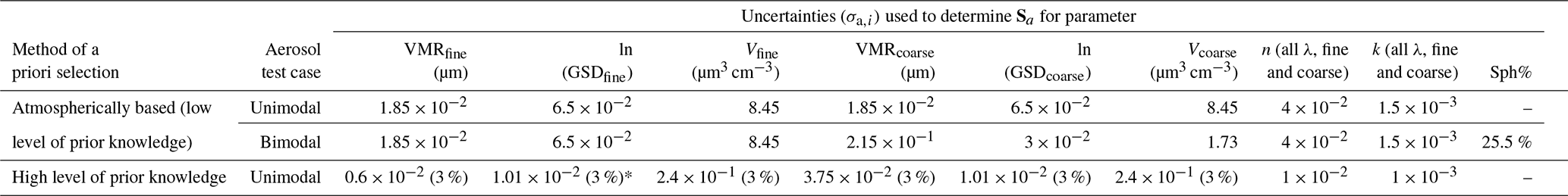
^∗ For the test cases σ_ln(GSD) of 3 % is equivalent to σ_GSD of ∼0.72 %.

We set the non-diagonal elements of S_a to 0, which amounts to the assumption that there is no covariance between the different aerosol state parameters. This simplifying assumption is common in information content analysis (Xu and Wang, 2015; Chen et al., 2017; Knobelspiesse and Nag, 2018; Burton et al., 2016). However, it should be noted that this is indeed a simplification for certain state parameters. For example, refractive index values (n or k) at different wavelengths are not completely independent of each other (Gao et al., 2018; Xu et al., 2019).

3.5 Forward model

To simulate the polarimetric measurement data (PF (θ, λ), PPF (θ, λ)) for given aerosol test cases, the forward module of the GRASP-OPEN algorithm was employed. GRASP-OPEN is a robust and well-established inversion algorithm that has been used extensively in the aerosol remote-sensing community (Dubovik et al., 2014, 2021) as well as for retrieving aerosol properties from in situ measurements (Schuster et al., 2019; Espinosa et al., 2019). In addition to its main application as an aerosol retrieval tool, GRASP-OPEN can be run as an independent physics-based forward module. The forward module of GRASP-OPEN is quite versatile and flexible, enabling use of either binned or multi-modal log-normal representation of the size distribution in state parameter space. Another advantage of GRASP-OPEN is that in addition to the basic, spherical-particle option, it also includes the option of considering non-spherical particle shape using the spheroid-based approach and the Sph% parameter discussed in Sect. 3.3.1. Therefore, all the state parameters assumed in our aerosol test cases are available in the state space implemented in GRASP-OPEN. The simulated PF (θ, λ) functions correspond to absolute phase functions with units of inverse megametres (Mm⁻¹): they are normalized such that the integral over the solid angle equates to 4πβ_scat, where β_scat is the integrated scattering coefficient. GRASP-OPEN also provides the Jacobian matrix, K, of the forward model for given aerosol states, which is required for computing information content.

3.6 Optimal angular sensor placement based on information content analysis

In this part of the study, we investigated to what extent particular choices of sensor placement affect the information content of polarimetric measurements. Building up on this, we introduced a method to identify optimal sensor placement for exemplary target aerosol states and instrument configurations. We constrained this analysis to unimodal, non-absorbing-aerosol models measured with single-wavelength instruments with either radiometric or polarimetric capabilities. A total of N_p=171 available angular positions were chosen at every full degree between θ=5 to 175^∘. The number of actually available sensors was then varied by considering eight cases with N_θ=2, 3, 6, 11, 18, 35, 86, and 169. This allowed us to assess the sensitivity of information content to sensor placement as a function of the number of available sensors.

Monte Carlo simulations were first conducted to randomly generate different angular sensor placements. Specifically, 1000 random draws of N_θ angles out of all the 171 available positions were made for every N_θ value. The DOFS values were calculated for all the randomly generated instrument configurations. This approach is not very efficient, but it does provide information on optimal sensor placement if the number of random draws is sufficiently high. As a proof of concept, we also developed and tested a potentially more efficient approach to obtain the optimal angular sensor placement based on the reductive greedy algorithm, which is a well-known and robust optimization scheme. The greedy algorithm was applied to this optimization problem by incorporating DOFS calculations into the algorithm scheme. Specifically, the algorithm was set up to selectively remove angular positions corresponding to the smallest changes in DOFS until only the most informative angles remained in a particular configuration. The full pseudo-code for the algorithm is detailed in Sect. S1 in the Supplement.

4 Results and discussion

4.1 Dependence of information content on the angular configurations of previous polar nephelometer designs

Here we assess how the information content increases with an increasing number of angular data points for the angular configurations of four polar nephelometer designs previously reported in the literature (Li et al., 2019; Nakagawa et al., 2016; Dolgos and Martins, 2014; Dick et al., 2007). For each of these angular configurations, different spectral and polarimetric capabilities are considered (specifically, all four combinations of data sets that would be obtained with single/triple wavelength and radiometric/polarimetric measurements). The metric nDOFS (Table 1) was calculated for the fine, unimodal, non-absorbing-aerosol test case using the atmospherically based a priori covariance matrix given in Table 5.

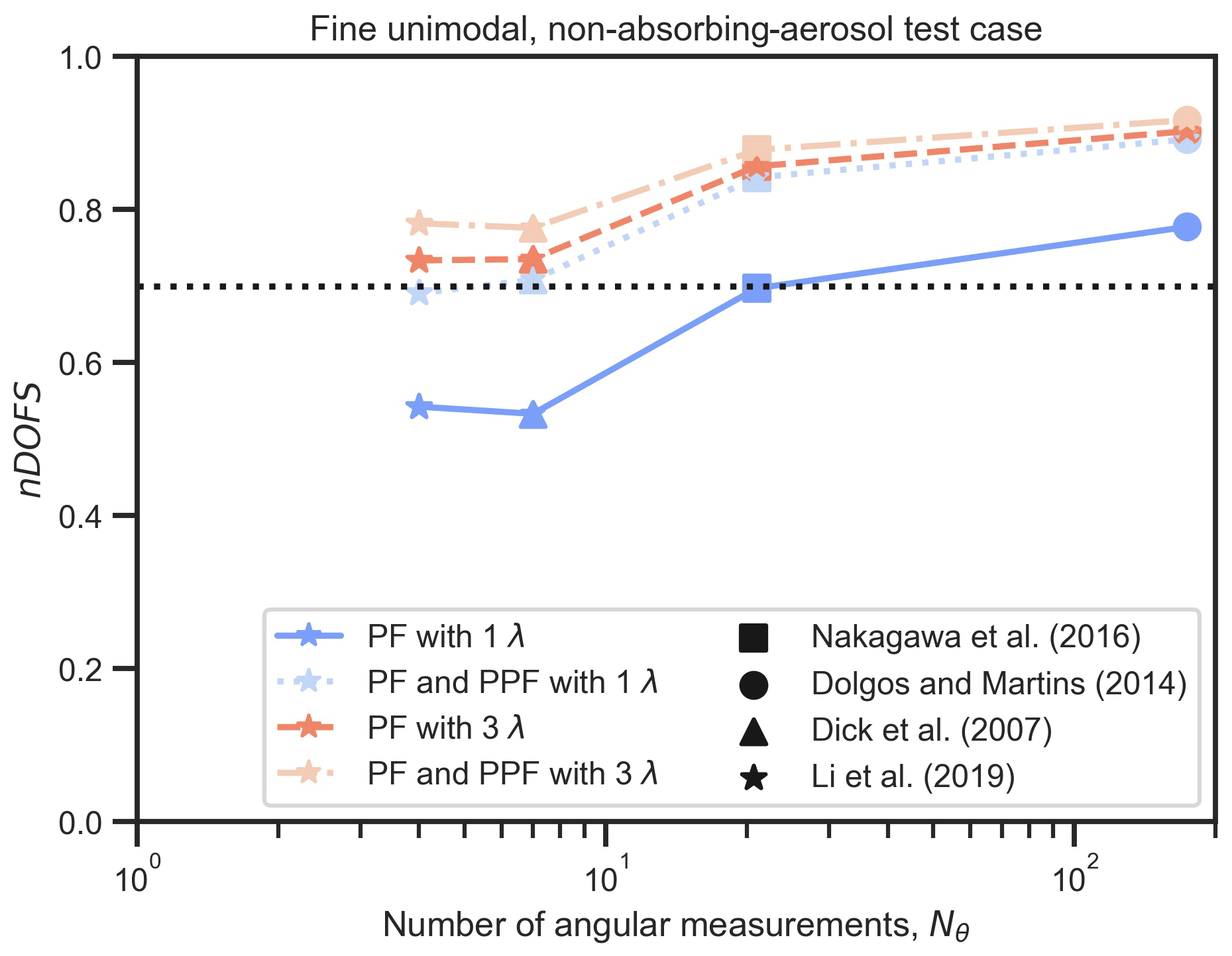
Figure 3 Variation in nDOFS for spectral polar, polarimetric, and angular configurations. The angular configurations are based on instruments available in the literature. The dotted line corresponds to nDOFS equalling 0.7 and is included for reference.

Figure 3 displays the comparison of the information content of data sets acquired by the above instruments. As expected, the nDOFS (ordinate) values generally increase with an increasing number of angular sensors (abscissa). However, this increase is not strictly monotonic. Specifically, data from the four-sensor instrument has comparable or even slightly higher nDOFS compared to the seven-sensor instrument depending on which spectral/polarimetric capabilities are considered. This suggests that implementing more sensors on its own is not necessarily enough to achieve more informative data and that the particular placement of the sensors may also be important. Comparable performance of the four- and seven-sensor instruments for the test aerosol case assessed here should not be interpreted in terms of better or poorer instrument design. Instead, the four-sensor instrument may be optimized for probing aerosols similar to this specific test aerosol case (unimodal, non-absorbing, fine-mode aerosol), whereas the seven-sensor instrument may be optimized for different target aerosol properties. The significance of sensor placement for different test aerosol properties and variable sensor number is explored in more detail in Sect. 4.8.

Figure 3 also shows that the addition of spectral and/or PPF measurement capabilities can result in DOFS increases that are comparable to the increases obtained by simply adding more angular sensors. For example, it can be seen that for this aerosol test case, the addition of polarization and/or multi-wavelength measurements will make the nDOFS values of instruments with four and seven angular sensors roughly equivalent to those of a single-wavelength instrument with 21 sensors without polarimetric measurement capabilities. In the following sections the effect of polarimetric, spectral, and angular measurement on the information content of a variety of retrievable state parameters is explored in more detail.

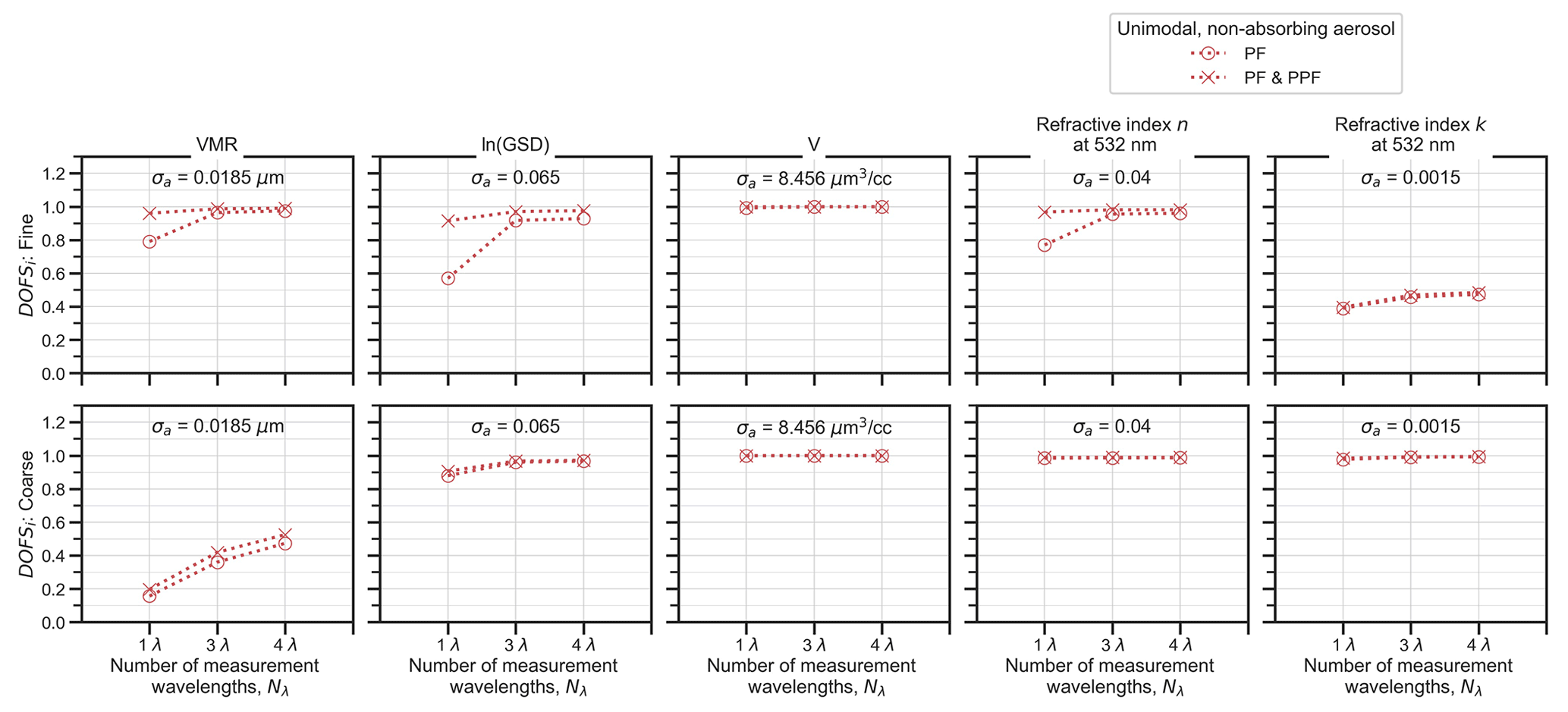
Figure 4 DOFS_i values for specific aerosol parameters corresponding to the fine (upper row) and coarse (bottom row) unimodal, non-absorbing-aerosol test cases. The a priori variance values are based on the atmospheric method described in Sect. 3.3 and the measurements from Espinosa et al. (2019).

4.2 Dependence of information content on the available prior knowledge of the aerosol state parameters

Polarimetry may be applied to a wide range of different aerosol types and in applications with different prior knowledge of the aerosol under investigation. Qualitatively speaking, the more prior knowledge is available on the state parameters of a certain aerosol, the more challenging it becomes to gain additional information through probing this aerosol with a polarimetric measurement. The DOFS-based information content metrics as introduced in Sect. 2 are one approach to quantify differences in information gain as a function of prior knowledge, instrument configuration, measurement error, and reference state of the probed aerosol (Fig. 1). Here we focus on the effect of prior knowledge of DOFS, which comes in through the a priori variance matrix (Eqs. 3 and 4), and how to interpret and compare resulting DOFS values. For this purpose we choose two distinct variants of a priori knowledge as detailed in Sect. 3.4. As for the measurement capabilities, we computed DOFS_i over different N_λ values (1λ, 3λ, 4λ; see Sect. 3.1.4) and polarimetric settings (radiometric or polarimetric) for a fixed angular configuration. Specifically, we selected a generic angular configuration with α=5^∘, $\mathit{\beta }=\mathrm{0}{}^{\circ }$, and Δθ of 10^∘ (which corresponds to N_θ=18) to represent a polar nephelometer with moderate detection angle resolution. We used the fine and coarse unimodal, non-absorbing-aerosol test cases for this investigation (see Sect. 3.3.2).

To address the measurement of largely unconstrained atmospheric aerosols, DOFS_i values were calculated using the atmospherically based a priori covariance matrix detailed in Table 5. That is, the aerosol state parameters were a priori assumed to vary over the ranges covered by the comprehensive ambient measurements reported by Espinosa et al. (2019). Figure 4 displays the DOFS_i results as a function of instrument capabilities as well as for fine and coarse test states of a unimodal aerosol. The results indicate that all the tested configurations provide high information content in this situation. For example, even the 1λ instrument produces DOFS_i values above 0.8 for the majority of the unimodal-aerosol state parameters (with the exceptions of VMR_coarse, ln(GSD)_fine, and k_fine). Values of DOFS_i greater than 0.8 indicate that the posterior value of a given retrievable parameter is driven almost entirely by the information a new measurement provides rather than by what is known a priori about that value. In this sense, these results demonstrate that even a single-wavelength polar nephelometer with moderate angular resolution will provide very informative measurements in relation to the expected variability in ambient aerosol properties. However, while this is a useful insight, the overall high DOFS_i values shown in Fig. 4 (i.e. very close to 1) impede the comparison of the different spectral and polarimetric instrument configurations.

The main reason that the DOFS_i are quite high over most of the state parameters is due to the assumption for the a priori variance values. DOFS_v is a prime example of a state parameter with DOFS_i very close to 1 for both fine and coarse cases. Such results suggest that even a basic polar nephelometer can provided ample information on aerosol properties when measured against prior knowledge that is as crude as “unimodal atmospheric aerosol with model diameter somewhere in fine or coarse mode”. This is not surprising given that the atmospherically based a priori variance for, e.g., the state parameter V (${\mathit{\sigma }}_{\mathrm{a}}{,}_V=\mathrm{8.5}$ µm³ cc⁻¹; Table 5) is larger than the actual reference value of V (8 µm³ cc⁻¹; Table 3) considered for all the unimodal test cases. It is worth mentioning that the ${\mathit{\sigma }}_{\mathrm{pro}}^{\mathrm{2}}/{\mathit{\sigma }}_{\mathrm{a}}^{\mathrm{2}}$ results, which are depicted in Fig. S1, show that for parameter V ${\mathit{\sigma }}_{\mathrm{pro}}^{\mathrm{2}}/{\mathit{\sigma }}_{\mathrm{a}}^{\mathrm{2}}$ decreases by a factor of ∼10 when the number of measurement wavelengths is increased from 1λ to 3λ. This demonstrates that despite the very high DOFS_v values already achieved by a single-wavelength instrument, the addition of spectral capabilities does actually substantially reduce the uncertainty in the retrieved state.

Results from Fig. 4 further suggest that the DOFS_VMR values for the fine case are systematically larger than those for the coarse case. In the DOFS_i calculations of Fig. 4, the absolute a priori variances for VMR in fine and coarse cases are identical. This means that relative to the given fine and coarse VMR state values (0.2 and 1.25 µm, respectively), the a priori variance fraction is much greater for the fine than for the coarse case. Therefore, the finding that DOFS_VMR is higher when probing the fine mode compared to probing the coarse mode within a given a priori range must not be interpreted as better performance relative to the retrieved VMR state values. An alternative approach, to make DOFS_VMR more comparable for different tested aerosol states, is to assume that the a priori variance is a percentage of the corresponding state parameter value (as listed in Table 5 for the size distribution state parameters). Figure S2 presents DOFS_VMR results for the two alternative a priori variances: that is, either the atmospheric range or as a fixed percentage of tested state representing a high level of prior knowledge. Indeed, it can be seen that by using percentage-based a priori variance, the DOFS_VMR values and trends with spectral capabilities become similar for fine and coarse test cases. These results imply that the polar nephelometer measurement is comparably informative in relative terms for retrieving VMR for both fine- and coarse-mode aerosol.

Using low percentages of the test case state parameter values as corresponding a priori ranges sets tighter bonds on the a priori knowledge compared to the wider atmospheric a priori range. This results in lower information content of identical measurements when expressed with DOFS_i. A side effect of shifting DOFS_i down to medium values is that DOFS_i becomes more sensitive to differences in instrument configurations and measurement precision for equal aerosol state test cases. Therefore, we chose the “high level of prior knowledge selection” method for computing DOFS_i in most of the following examples. For the size distribution state parameters, a constant percentage value of 3 % (as listed in Table 5) was chosen so that the majority of DOFS_i values over all instrument configurations and tested aerosol states does not assume extreme values near 0 nor near 1. For the refractive index state parameters, it was not possible to find a common percentage value that was meaningful for both the non-absorbing- and absorbing-aerosol test cases. Therefore, constant absolute a priori uncertainties were chosen for fine- and coarse-mode n and k (see Sect. 3.4 and Table 5).

Figure 5 is equivalent to Fig. 4 but shows DOFS_i values for the “high level of a priori knowledge selection” method for the unimodal-aerosol model. One of the very basic insights that can be drawn from this figure is that for given state parameters, DOFS_i always increases when the measurement configuration becomes more complex, be it through additional measurement of PPF or measurements at multiple wavelengths. However for some related pairs of data points, the DOFS_i increases can be very minor. For example in the coarse-mode case, DOFS_n increases by only 0.0006 when the number of measurement wavelengths is increased from 3λ to 4λ for a radiometric measurement (i.e. PF only). This indicates a potentially poor cost-to-benefit ratio of performing more complex measurements for accurate quantification of the corresponding state parameter.

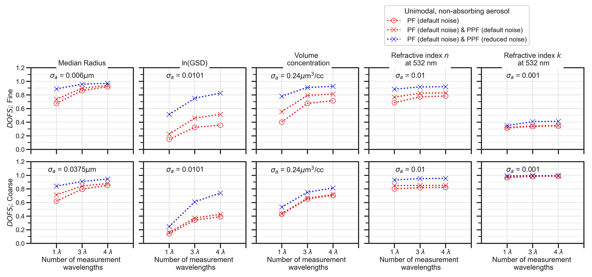
Figure 5 DOFS_i values for specific aerosol parameters corresponding to the fine (upper row) and coarse (bottom row) unimodal, non-absorbing-aerosol test cases. The a priori variances (σ_a) for each state space parameter are displayed as text boxes in each panel. These values were chosen according to the “high level of prior knowledge” selection method described in Sect. 3.3. The blue lines are the DOFS_i values corresponding to a reduced PPF measurement noise level of 0.01, while the default noise is 0.056 (Eq. 9). The relative PF measurement noise level is 0.046 (Eq. 8) for all curves.

Figure 5 also indicates that when the a priori variances are chosen as fixed percentage of the corresponding fine and coarse x_0,i values, then the trends and values of DOFS_i between fine and coarse test cases are quite similar for all aerosol parameters except the imaginary part of the refractive index k. This suggests that the finding from Fig. S2 for the VMR state parameter applies more generally to most state parameters: the polar nephelometer measurement is comparably informative in relative terms for most retrievable aerosol state parameters independently of whether one is probing fine or coarse unimodal aerosols. The exceptional behaviour of DOFS_k in this regard is explained in more detail in Sect. 4.4.

4.3 Information content gain associated with more comprehensive measurements and reduced measurement error

In Sect. 4.2 we explained that DOFS_i calculated with the “high level of prior knowledge” selection method is a sensitive metric to demonstrate the benefits of more comprehensive or more precise polarimetric measurements. Therefore, the DOFS_i results based on this variant of a priori knowledge that are presented in Fig. 5 are used for the following discussion.

4.3.1 Information content gain due to multi-wavelength measurements

Figure 5 indicates that increasing the number of measurement wavelengths can lead to noticeable information gain for all three size distribution parameters (mean radius, GSD, and volume concentration). For each of these parameters, DOFS_i for the 3λ instrument configurations are considerably higher compared to the single-wavelength configurations. For example, DOFS_ln(GSD) and DOFS_V increase by an absolute value of 0.22 (22 % of full DOFS_i scale) when going from a single to a 3λ instrument (for both fine and coarse cases).

The results further indicate that although the addition of infrared wavelength in 4λ also increases the DOFS_i values, such improvement is noticeably smaller than the DOFS_i improvement when transitioning from a 1λ to a 3λ configuration. For most of the test cases, the increase in information content when moving to a 4λ configuration was less than ∼40 % of the corresponding DOFS_i increase when transitioning from 1λ to 3λ. This observation suggests that the addition of a fourth wavelength measurement in the near IR is not very beneficial for the retrieval of the size distribution parameters of a unimodal, homogeneous, and spherical aerosol.

For the refractive index parameters, Fig. 5 suggests that the addition of multi-wavelength measurements only weakly increases information content with respect to the n and k values at the wavelength of the single-wavelength instrument (532 nm in this case). However, it should be noted that multi-wavelength measurements do increase information content in the sense that they enable the retrieval of refractive index values at the additional wavelengths that the measurements are performed at (e.g. this is shown for DOFS_n values at 450, 532, 630, and 1020 nm in Fig. S3). This is a trivial result that simply expresses the expectation that adding measurement wavelengths to a given instrument configuration brings information about the refractive index values at the added wavelengths.

4.3.2 Information content gain due to polarimetric measurements and reduced measurement error

Comparing the curves with red circles and red crosses in Fig. 5 provides an insight into the information content benefit of adding PPF measurements with an absolute error of 0.056 (Eq. 9). This level of absolute PPF measurement error is based on the laser imaging nephelometer of Dolgos and Martins (2014). For this case, the addition of PPF results in an only minor DOFS_i increase (at most ∼0.15) across all the λ configurations for fine-mode volume concentration and ln(GSD). For all other parameters the DOFS_i increases were even lower. By contrast, the corresponding DOFS_i increases when transitioning from a 1λ to a 3λ instrument configuration are considerably larger.

In the context of remote-sensing instrumentation, PPF measurement errors can be considerably lower than the default noise level of 0.056 that is considered here. For example, Xu and Wang (2015) consider an absolute error of 0.01 for polarized measurements made by AERONET sun photometers. The blue curves in Fig. 5 demonstrate the information content benefit of adding PPF measurements with such a reduced absolute error (e.g. 0.01 rather than 0.056) while retaining the PF noise level unchanged. This change results in a substantial information content increase over all state parameters and wavelength numbers, with the exception of V (coarse) and k (coarse and fine). With the reduced level of noise in the PPF data, a single λ instrument with polarimetric capability could be similarly or even more informative than a 4λ instrument with PF measurement only (e.g. see the DOFS_i values for the size distribution parameters of the fine test case in Fig. 5).

It should be noted that all of the results shown so far are valid for probing rather simple aerosol systems, i.e. unimodal size distributions of spherical particles with homogeneous optical properties. For more complex aerosols the information content benefit associated with the addition of polarimetric measurements can be even higher, as we demonstrate below in Sect. 4.5.

4.4 Information content for the imaginary part of the refractive index

Light absorbing aerosols are found ubiquitously throughout the atmosphere. Retrieving information on light absorption by an aerosol from polarimetric light scattering data is known to be difficult and can require the use of additional independent measurements as constraints (e.g. Espinosa et al., 2019). Nevertheless, the results shown in Fig. 5 for DOFS_k for the non-absorbing-aerosol case demonstrate that some information can be retrieved. In the following, we assess how this depends on the actual aerosol test case.

Figure S5 displays the same results shown in Fig. 5 but for the absorbing-aerosol test case. Comparing the two figures, it can be seen that the DOFS_k values for non-absorbing aerosols are larger than the corresponding values for absorbing aerosols when assuming identical σ_a,k. This demonstrates that it is possible to retrieve the k of non-absorbing aerosol with slightly more absolute precision than the k of absorbing aerosol, for the reasons explained below.

A further result seen in both Figs. 5 and S5 is that there are considerable systematic differences in DOFS_k between the coarse- and fine-aerosol cases, i.e. the polarimetric light scattering measurement is much more informative regarding k for coarse aerosol compared to fine aerosol (using otherwise equal aerosol state parameters). In contrast, the DOFS_i values of all of the other aerosol state parameters are comparable between corresponding fine and coarse test cases. The greater DOFS_k values for coarse compared to fine aerosol are consistent with previous phase function sensitivity calculations (see Figs. 1 and 2 in Espinosa et al., 2019).

DOFS_k values noticeably greater than 0 are obtained except for the fine-mode absorbing example, which suggests that even under the assumption of very high prior knowledge of k, angularly resolved light scattering measurements can still contribute additional information about aerosol absorption. For example, the DOFS_k values for the non-absorbing, coarse-aerosol case are unity, which suggests that for this simple unimodal aerosol and assumed measurement uncertainty, it should be possible to retrieve k to a precision better than three decimal places (i.e. given that the a priori uncertainty σ_a,k is 0.001).

To explore these findings in more detail, we further assess the sensitivity of phase function to k using the absolute value of the error-corrected Jacobian (K_EN, i), which was introduced by Xu and Wang (2015) for a given state parameter x_i based on the following formula:

$$\begin{array}{}\text{(13)}& {\mathbf{K}}_{\mathrm{EN},i}=\mathrm{|}\left({\displaystyle \frac{\partial \mathbf{y}}{\partial x_i}}\right)\times \left({\displaystyle \frac{{\mathit{\sigma }}_{\mathrm{a},i}}{{\mathit{\sigma }}_{\mathrm{meas}}}}\right)\mathrm{|},\end{array}$$

where y is either the PF or PPF measurement vector, ${\mathit{\sigma }}_{\mathrm{a},i,}$ is the square root of a priori variance for parameter x_i, and σ_meas is the vector of measurement uncertainties. K_EN,i can be interpreted as a normalized partial derivative of PF (or PPF) with respect to x_i, which is a measure of the measurement sensitivity to perturbation in state parameter x_i. Figure S4b shows the results of K_EN,k as a function of scattering angle for the four combinations of fine and coarse as well as non-absorbing and absorbing test cases. The results indicate that for the equally complex refractive index, the coarse-aerosol cases have larger normalized derivative values than their fine counterparts at the majority of scattering angles, which is consistent with higher DOFS_k. We suggest that the greater amount of internal light absorption within coarse versus fine particles has a stronger feedback on internal light intensity and hence greater perturbation of the external scattered light field for an equal change in k.

Although K_EN,k as displayed in Fig. S4b is useful for gaining an overview on measurement sensitivity to state parameter perturbation, the results are not always sufficient for the interpretation of DOFS and information content. This is due to the fact that the Bayesian approach accounts for inter-dependence of information content across different state parameters. However, the DOFS_i of parameters other than k is rather insensitive to changing k in the aerosol test case, which can be seen when comparing Figs. 5 and S5. Therefore, using K_EN,k should lead to comparable results to the DOFS_k metrics. Indeed, the four test cases exhibit a consistent order when assessed with these two metrics (cf. Fig. S4a and b).

The results presented here demonstrate that polarimetric measurements can be very informative on k when probing simple aerosols. However, atmospheric aerosol samples are much more complex in terms of size-dependent composition, mixing state, and particle shape. This considerably reduces the information content of polarimetric measurements with respect to light absorption.

4.5 Information content for the bimodal non-spherical-aerosol model

The more complex an aerosol, the more state parameters are required to describe it. Retrieving the state parameters of more complex aerosols from polarimetric measurements will, accordingly, require data with overall higher information content. This may amplify the benefit of performing measurements with instruments that have more comprehensive capabilities or smaller measurement errors. To address this hypothesis, we used the bimodal non-spherical-aerosol model with two test cases based on the results from Espinosa et al. (2019). These two cases represent “urban” and “dust-dominated” aerosols measured over the USA. The DOFS values are calculated using the atmospherically based a priori variance assumptions and the default noise level for PPF (i.e. 0.056). The results are shown in Fig. 6. It should be reiterated that for these analyses the a priori variances assumed for coarse- and fine-size distribution parameters are not identical. For example, the a priori variance for a coarse median radius is ∼130 times larger than the fine median radius. Hence, DOFS_i should not be compared in absolute terms between fine and coarse test cases.

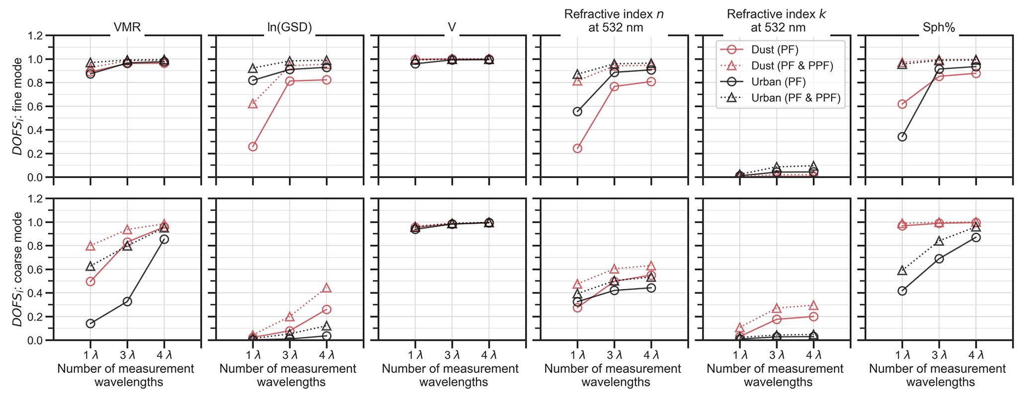
Figure 6 DOFS_i values for specific aerosol parameters corresponding to the fine (upper row) and coarse (bottom row) bimodal non-spherical-aerosol model with a priori variance values based on results from Espinosa et al. (2019).

The DOFS_i results from the bimodal test cases indicate that both multi-wavelength and PPF measurements can greatly increase the retrievable information about aerosol shape. For example, the addition of PPF measurement (triangle markers) results in DOFS_Sph% for fine-mode values becoming greater than 0.9 for both aerosol test cases, even though the PPF measurement error is assumed to be high. The effect of PPF measurement on DOFS_Sph% is weaker in coarse aerosol. On the other hand, the transition from 1λ to 3λ can also increase the DOFS_Sph% considerably, for example up to differences of 0.3 for the coarse mode and 0.6 for the fine mode. The fourth λ further increases the DOFS_Sph% unless values near 1 are already reached with the three λ variants.

The results further show strong DOFS_n improvements (fine and coarse) when transitioning from 1λ to 3λ, while the benefit starts to level off at the fourth wavelength. Furthermore, the benefit of adding PPF measurements is also highlighted by the substantial DOFS_i increases achieved for n as well as the size distribution parameters (VMR, ln(GSD)), especially for the 1λ instrument configuration. Overall, the complexity of the bimodal aerosol model including a non-spherical shape parameter (Sph%) raises the polarimetric challenge to a level where performing more comprehensive measurements in terms of spectral and/or polarimetric capabilities clearly benefits the achieved information content and hence the retrievability of state parameters.

4.6 Dependence of information content on angular measurement truncation

As described in Sect. 3.1, angular truncation in nephelometry refers to the inability of measuring light scattering at certain angles due to physical design limitations. To investigate the effect of truncation on aerosol property retrieval potential, we used two simplified aerosol tests cases (fine and coarse unimodal, non-absorbing, spherical particles) and two measurement configurations: a basic instrument (Δθ=1^∘, 1λ, and PF only) and a comprehensive instrument (Δθ=1^∘, 4λ, and PF and PPF). For all of these cases, we employed the default measurement noise setting (e.g. relative PF measurement error of 0.046, and absolute PPF measurement error of 0.056), and the “high level of prior knowledge” method for selecting a priori variances.

4.6.1 Extreme-angle truncation

Figure 7 demonstrates the effect of extreme-angle truncation α (i.e. loss of light scattering data at extreme forward and backward angles) on DOFS_i for the five unimodal-aerosol state parameters. As expected, in all of the simulated cases, DOFS_i decreases as α increases and measurement information is lost. Generally, the DOFS_i values for the fine test cases decrease less than the corresponding values for the coarse test cases. For the fine case with basic instrument configuration, only DOFS_VMR and DOFS_k display notable sensitivity to α, decreasing by ∼0.4 and ∼0.3, respectively, when α is increased from 0 to 40^∘. The extreme-angle truncation effect on DOFS_VMR can even be largely avoided by the use of the comprehensive 4λ, polarimetric instrument configuration. However, this more comprehensive instrument configuration has little effect on the truncation effect for DOFS_k. Overall, the relative insensitivity of fine-mode DOFS_i (excepting DOFS_k) to the loss of measurement information at forward and backward angles can be understood by the fact that the scattering phase functions of fine-mode aerosols are relatively isotropic, with no distinct features in the extreme-angle scattering directions.

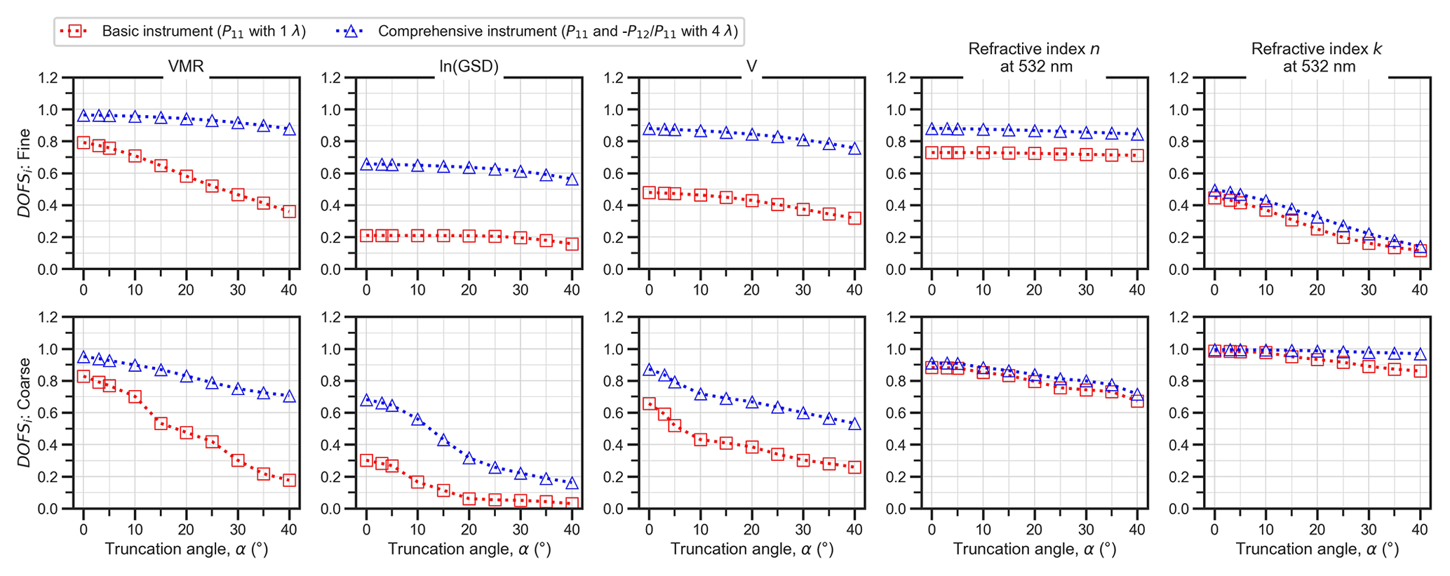
Figure 7 Variation in DOFS_i for unimodal, non-absorbing-aerosol test cases over different extreme-angle truncation cases. The top row demonstrates the results for the fine-aerosol test case, while the bottom row corresponds to results for the coarse-aerosol test case. These results were obtained using default measurement noise values and the “high level of prior knowledge” method for selecting a priori variances.

In contrast to the fine test case, Fig. 7 indicates that DOFS_i for the coarse test case is relatively sensitive to α for all five unimodal-aerosol state parameters. For the basic instrument configuration, DOFS_i for all state parameters decreased by at least 0.1 when α was increased from 0 to 40^∘. Furthermore, the addition of multi-wavelength and polarimetric capability with the comprehensive instrument configuration did little to change these trends, except for the state parameter k where a noticeable improvement was observed. The differing response to extreme-angle truncation for simple coarse-mode aerosols compared to fine-mode aerosols can be explained by the fact that the phase functions of spherical, coarse particles are relatively more forward-focused than those of spherical, fine particles, and, therefore, the loss of measurement information at extreme forward angles has a greater effect on the retrievability of the coarse-aerosol properties.

This information content analysis of the extreme-angle truncation effect has implications for polar nephelometer design. For example, if an instrument is being designed to measure both fine and coarse aerosols, then minimizing extreme-angle truncation as much as technically possible is a beneficial aim. However, if an instrument is being designed to measure only simple, fine-aerosol particles (i.e. without complex shapes), then one should aim to include multi-wavelength and polarimetric measurement capabilities rather than expending considerable design effort on minimizing extreme-angle truncation.

4.6.2 Side scattering truncation

As explained in Sect. 3.1.2, some polar nephelometers suffer from side angle truncation (i.e. the loss of scattering information at scattering angles around 90^∘, which we denote with the angle β). Figure 8 demonstrates the effect of side angle truncation on DOFS_i for the five unimodal-aerosol state parameters. For all five of the parameters, only relatively minor decreases in DOFS_i (<0.25) are observed when β is increased, even when it is set to very large values of 40^∘. This finding is valid for both fine- and coarse-mode aerosols and for both basic and comprehensive (i.e. polarimetric) instrument configurations. This suggests that in contrast to extreme-angle truncation (Fig. 7), side angle truncation has little effect on the ability to retrieve fine- and coarse-mode aerosol properties from polar nephelometer data.

Figure 8 Variation in DOFS_i for unimodal, non-absorbing-aerosol test cases over different side-truncation angles. The top row demonstrates the results for the fine-aerosol test case, while the bottom row corresponds to results for the coarse-aerosol test case. These results were obtained using default measurement noise values and the “high level of prior knowledge” method for selecting a priori variances.

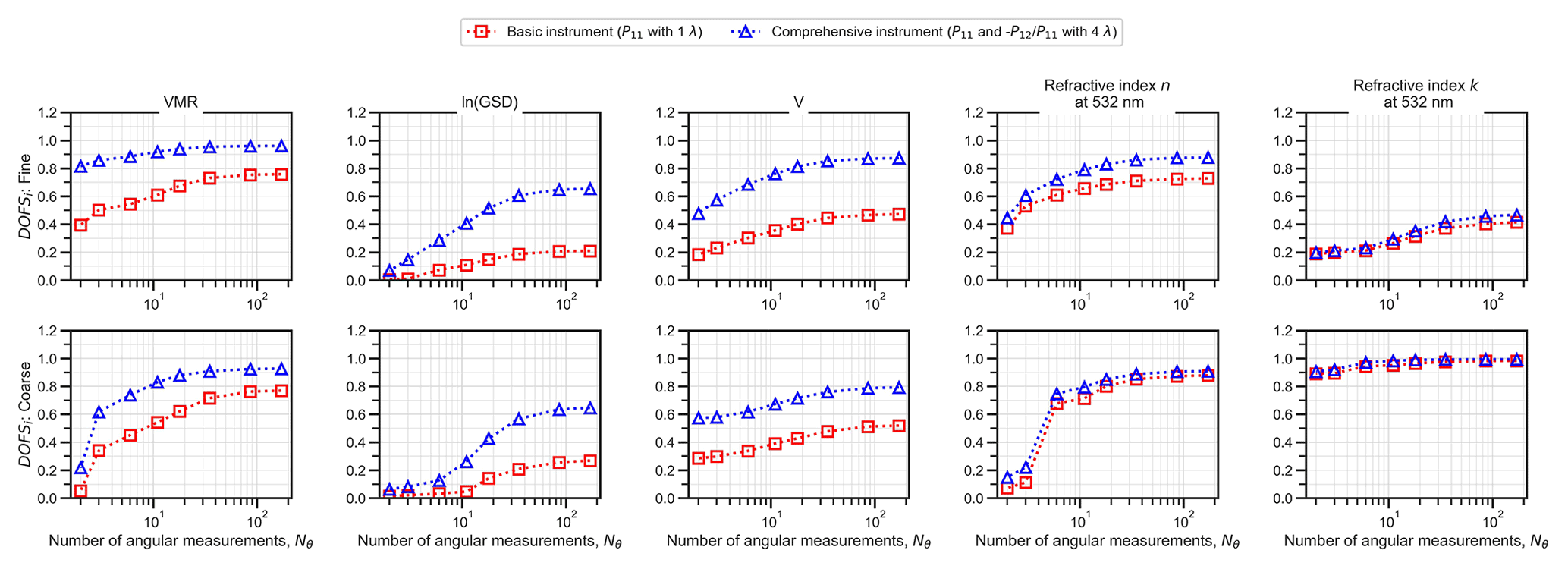
Figure 9 Variation in DOFS_i for unimodal, non-absorbing-aerosol test cases as a function of the number of angular measurements N_θ. The top row demonstrates the results for the fine-aerosol test case, while the bottom row corresponds to results for the coarse-aerosol test case. These results were obtained using default measurement noise values and the “high level of prior knowledge” method for selecting a priori variances.

4.7 Dependence of information content on the number of angular measurements

The number of angular measurements, N_θ, is a central design feature of polar nephelometer instruments. N_θ can vary greatly – from 4 or lower for fixed detector systems (Nakagawa et al., 2016) up to 174 for laser imaging nephelometers (Dolgos and Martins, 2014) – and it has a substantial impact on the overall information content of polarimetric data as discussed in Sect. 4.1 using the metric nDOFS. Here we assess the effect of different N_θ on information content regarding individual aerosol state parameters in more detail using the DOFS_i metrics. For this purpose, we consider eight different angular detection configurations with N_θ ranging from 2 to 171. In each of the eight configurations, the detection angle locations are evenly distributed (see Sect. 3.1.3 and Table 2). As in Sect. 4.6, for these simulations we used two simplified aerosol tests cases (fine- and coarse-mode unimodal, non-absorbing, spherical particles), two measurement configurations (a basic instrument with 1λ and PF only and a comprehensive instrument with 4λ and PF and PPF; in each case α=5^∘ and β=0^∘), default measurement noise values, and the “high level of prior knowledge” method for selecting a priori variances.

Figure 9 displays DOFS_i as a function of the number of angular measurements N_θ for five unimodal-aerosol state parameters (three size distribution parameters and two refractive index parameters for the wavelength of the 1λ instrument). For all of the parameters, DOFS_i increases as N_θ increases; i.e. all DOFS_i contribute to the increase in overall nDOFS with increasing N_θ as shown in Fig. 3. Interestingly, the DOFS_i values tend to begin plateauing out at N_θ values of around 20–40. This indicates that for the investigated combination of relatively simple aerosol models, high a priori knowledge (i.e. small a priori variance), and default measurement noise, excessive angular resolution does not result in substantial information gain. If N_θ already falls into the plateau range, then information content can still be increased by the addition of multi-wavelength and polarimetric measurement capabilities (blue curves in Fig. 9). Based on results in the previous sections, it can be expected that the plateau in information content as a function of N_θ shifts to higher N_θ values, e.g. for more complex aerosol models or smaller measurement noise. However, quantitative validation of this hypothesis is beyond the scope of the current work. Finally, it should be noted that these results only apply to polydisperse aerosol size distributions. Information content and its dependence on instrument design features differs considerably when probing narrow size distributions with more pronounced angular features in the polarized phase function.

Finally, it should be noted that for some of the instrument configurations considered in this N_θ analysis, the dimension of observation become smaller than the number of retrievable parameters, resulting in an underdetermined inverse problem. This is noticeable for N_θ<6, where drastic reductions in DOFS_i values are observed for all state parameters, especially for the basic instrument configuration with PF only at 1λ. For such underdetermined cases, the maximum possible value of the sum of DOFS_i over all state parameters is equal to the observation dimension rather than the number of retrievable parameters (Rodgers, 2000). For example, in Fig. 9, it can be seen that for the basic instrument configuration with N_θ=2, the sum of all fine-mode DOFS_i values is 1.14 (DOFS_VMR=0.39, DOFS_ln(GSD)=0.0044, DOFS_V=0.184, DOFS_n=0.371, DOFS_k=0.188), which is less than the observation dimension of 2.

4.8 Proof of concept for using DOFS as metric for optimizing detection angle placement

In the previous Sect. 4.7, N_θ was varied while assuming that the angular measurements were evenly distributed across the full range of scattering angles θ. Equidistant detection angle placement has often been applied to the design of fixed-detector-type polar nephelometers (e.g. Nakagawa et al., 2016). However, one might expect that for low values of N_θ, the specific locations of the different angular measurements/detection angles within the scattering angle range will also be an important handle to maximize information content. To explore the potential benefit of optimized detection angle placement, we conducted a Monte Carlo simulation where we computed nDOFS for 1000 different random detection angle placement configurations given eight different N_θ values (see Sect. 3.5). For this analysis we used a basic aerosol model (unimodal size distribution) and assessed two state cases (fine and coarse, non-absorbing, spherical particles) and one measurement configuration corresponding to the basic polar nephelometer design (single wavelength, PF, and PPF).

Figure 10a and b show the results of the Monte Carlo simulations as grey markers for both the fine and coarse test cases, respectively. At a given N_θ, the grey markers spread over a range of nDOFS values. For example, for the coarse test case with N_θ=11, nDOFS varies from ∼0.3 to 0.6 across the 1000 randomly generated detection angle placements, which implies that choosing the optimal detection angle placement could substantially increase information content and thus retrievability of state parameters. Generally, this spread in nDOFS values becomes greater as N_θ decreases. This confirms the suppositions that, first, actual detection angle location is important and, second, the potential benefit of optimizing detection angle location increases with decreasing values of N_θ. Furthermore, the Monte Carlo results demonstrate that the spreads in nDOFS values are smaller for the fine-mode test cases than the corresponding coarse test cases. Therefore for a given N_θ value, choosing the right detection angle placement is more critical if one seeks to measure coarse rather than fine particles.

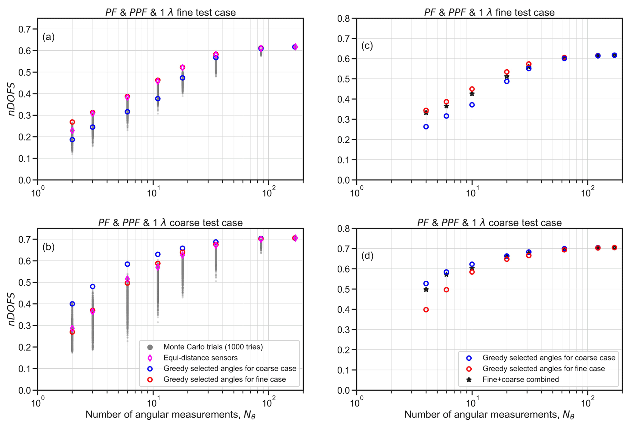
Figure 10 Panels (a) and (b) show the nDOFS values for optimized angular configurations for different detection angle numbers based on reductive greedy algorithms. The red points correspond to optimized configurations of the fine-aerosol test case, while the blue points correspond to the optimal detection angle configuration of the coarse-aerosol case. The grey dots are results of Monte Carlo simulations of 1000 random angular configurations for each case of detection angle numbers. In (c) and (d) the black dots correspond to the normalized nDOFS values for the combined optimal configurations of fine and coarse test cases.

While the Monte Carlo method suggests a brute force approach to the task of identifying optimal detection angle placements, we also present here a proof of concept analysis showing how a conventional optimization method could be applied to this problem. For this purpose we employ the reductive greedy algorithm described in Sect. 3.5. The nDOFS values corresponding to the detection angle placements determined by the greedy algorithm are also displayed in Fig. 10. The algorithm was applied separately to the fine-mode (red open markers) and coarse-mode (blue open markers) test cases. To place these results in further context, the corresponding nDOFS values for equidistantly placed detection angles are also displayed in Fig. 10a and b as purple open markers. The greedy algorithm performs excellently for both the fine and coarse test cases: it is able to identify detection angle placements that produce nDOFS values that are greater than the corresponding values for equidistantly placed detection angles and that are similar to the upper bounds of Monte Carlo-simulated configurations, regardless of the given N_θ value. Indeed for the coarse-mode test case (Fig. 10b), the greedy-simulated nDOFS values are even greater than the upper bound of the Monte Carlo-simulated values. We speculate that this is because the number of Monte Carlo tries (1000) was not sufficient to generate a random detection angle configuration matching the optimal configuration.

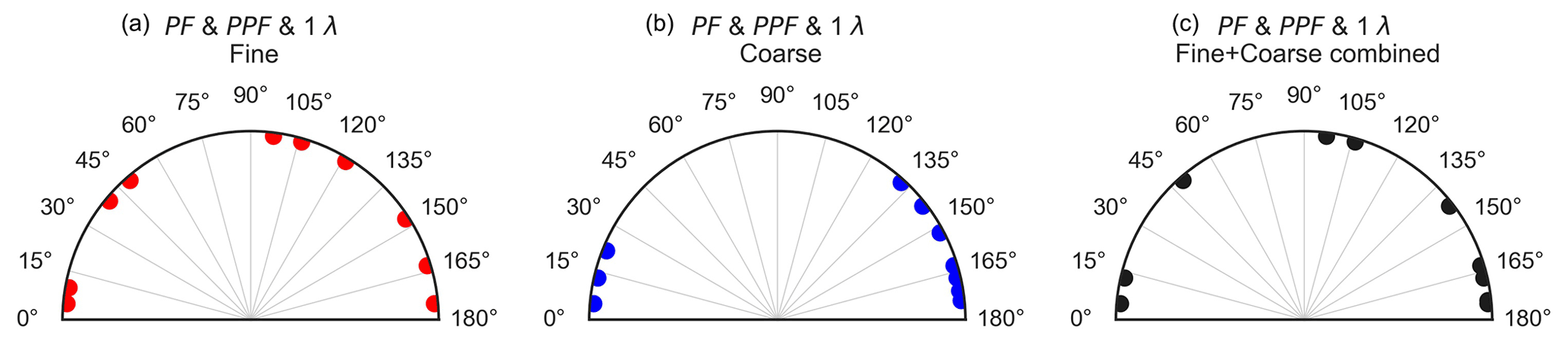
Figure 11 Panels (a) and (b) are optimal detection angle locations for the fine- and coarse-aerosol test cases, respectively, with phase function only and phase function and polarized phase function measurement cases. Panel (c) is the angular configuration constructed by combing fine and coarse configurations with q=6 configurations; due to a common angle point, the resulting configuration has N_comb=10.

The question then arises as to how the optimal detection angle locations determined for the fine-mode aerosol test case compare with those determined for the coarse-mode case. Figure 11a and b display these optimal detection angle locations for N_θ=10 (given the same basic, 1λ, PF, and PPF instrument configuration simulated in Fig. 10). In the fine-mode case (Fig. 11a), the 10 angular measurements/detection angles are distributed relatively evenly across the full scattering angle range. However for the coarse-mode case, the detection angles are concentrated in the forward and backward scattering directions. These differences are also reflected in Fig. 10a and b, which show that the differences between the greedy-simulated nDOFS values and the equidistant nDOFS values are much smaller for the fine than the coarse test case. The different optimal detection angle locations can be explained by the differences in the scattering phase functions of the respective test cases: specifically, the scattering phase functions of coarse-mode aerosol particles are more forward focused and less isotropic than those of fine-mode particles. This finding is consistent with the result presented in Sect. 4.6.1 that the retrievals of coarse-mode aerosol properties are more sensitive to extreme-angle truncation than retrievals of fine-mode properties.

Given the differences in the optimal detection angle locations for the fine- and coarse-mode aerosol test cases, it can be expected that using the optimally determined placements for one aerosol test case will produce suboptimal results when applied to the other aerosol test case. Figure 10a and b indicate that this is indeed the case. The optimal coarse-mode detection angle placements produce nDOFS values that are substantially lower than the optimal values when applied to the fine-mode aerosol test case (Fig. 10a) and vice versa (Fig. 10b). In both cases, even the equidistantly placed detection angle configuration yields higher nDOFS values than using the optimal detection angle placement of the wrong aerosol test case.

To mitigate this problem, one might attempt to combine the optimal detection angle placements for both cases to create an instrument that has similarly high information content with respect to the measurement of both fine- and coarse-mode particles. To investigate this approach we created combined optimal configurations at each value of N_θ that were composed of optimal fine and coarse configurations. For example, to create the combined optimal configuration with N_θ=10, the optimal fine and coarse configurations with N_θ=6 were joined together (since there were two commonly selected angles in both of these configurations, the total number of unique detection angles was only 10). The optimal detection angle locations for this combined configuration are displayed in Fig. 11c. This example shows that the combination method produces configurations that are less isotropic than the corresponding optimal fine-mode configuration but not as forward-focused as the corresponding optimal coarse-mode configuration. Figure 10c and d plot the nDOFS values that are yielded from the optimal combined configurations as black star markers for the fine- and coarse-mode test cases, respectively. Generally, it is seen that the combined configurations produce nDOFS values that are only slightly suboptimal. This suggests that combining optimal configurations for different aerosol test cases is a promising approach for designing instrument configurations that are suitable for measuring a broader range of different aerosol types.

In this section we have used a case study to demonstrate that DOFS is a useful metric for optimizing the detection angle placement in a polar nephelometer. Furthermore, we have shown that the optimal placements derived for the measurement of one type of aerosol will not necessarily coincide with the optimal placements determined for another aerosol type. As a final point, it should be stressed that these findings are only relevant at low values of N_θ, i.e. for fixed-detector systems. When the number of angular measurements is large, as in a laser imaging nephelometer, then there is no need to optimize the specific locations of those measurements.

5 Conclusions

Polar nephelometer designs can vary greatly in terms of spectral and polarimetric characteristics, as well as the number of angular measurements, their possible truncation, and their specific locations. These variations affect how much information can be retrieved from polar nephelometer measurements about the value of specific aerosol properties. To quantify these effects, we conducted a Bayesian sensitivity analysis to calculate an information content metric, DOFS, for a range of polar nephelometer instrument configurations, target aerosol cases, and assumed levels of measurement uncertainty and a priori knowledge. The majority of our analysis was focused on simulating the measurement of unimodal spherical aerosols described by three size distribution parameters (VMR, GSD, V) and 2N_λ refractive index parameters n(λ) and k(λ) (where N_λ is the number of measurement wavelengths of the simulated polar nephelometer design). Given prior knowledge of the ranges of variability of these parameters in the atmosphere (Espinosa et al., 2019), the information content analysis yields DOFS_i values near 1 for all of the parameters, even for a single-wavelength polar nephelometer with no polarimetric capability. This suggests that even very basic polar nephelometers will provide useful, retrievable information when used for atmospheric measurements.

To assess the benefit of polarimetric measurements for experiments with high prior knowledge of aerosol state parameters and to ensure consistent comparison of the size distribution parameters across the fine and coarse cases, we additionally employed an a priori covariance matrix which was more stringent than the corresponding atmospherically based a priori matrix. This led to a noticeable reduction in DOFS_i over most state parameters and configurations. Consequently, the “high level of prior knowledge” method facilitated distinguishing between the information content of different instrument configurations. With this a priori selection method, DOFS_i always increases as the measurement configuration becomes more comprehensive, either through the addition of PPF and/or through the addition of multiple measurement wavelengths. However, in some cases the observed DOFS_i increases are negligible, suggesting a poor cost-to-benefit ratio for such added measurements. Adding extra measurement wavelengths to a 1λ configuration can significantly improve the information content for size distribution parameters (mean radius, GSD, and volume concentration). However, the addition of an IR wavelength to the 3λ setup (i.e. to make a 4λ instrument) proved to be less beneficial in increasing DOFS_i. Furthermore, the PPF measurements appeared to be generally less informative using measurement error assumptions derived from an existing in situ instrument (Dolgos and Martins, 2014). However if the noise level is sufficiently low, PPF measurements can significantly improve the information content over all the state parameters. For some parameters, this even results in DOFS_i values for a 1λ instrument with PPF measurement capability that are similar to the corresponding values for a 3λ or 4λ instrument with PF measurement only.

Comparing absorbing vs. non-absorbing unimodal-aerosol test cases revealed the unique nature of the state parameter k. In particular, DOFS_k values are systematically larger for coarse- rather than fine-aerosol test cases. We demonstrated that this is because the PF's of coarse particles are more sensitive to perturbations in k than the PF's of fine particles Similar behaviour was not observed for any of the other state parameters.

By considering a more complex bimodal non-spherical-aerosol model, we showed that conducting more comprehensive spectral and PPF measurements can substantially improve the information content of different state parameters, such as n and Sph%.

We investigated the dependence of information content on angular truncation. For truncation in extreme forward and backward direction, DOFS_i values generally decrease as the truncation angle increases, particularly for the coarse-aerosol test cases. In contrast to the extreme truncation, the side truncation appears to have no significant impact on DOFS_i reduction in both fine and coarse test cases. To investigate the dependence of information content on the number of angular measurements N_θ we varied this parameter from 2 to 171. DOFS_i increased with increasing N_θ over all the state parameters but began to plateau out at N_θ values of around 20–40. This suggests that for the specific investigated cases, improving the angular resolution above a certain point does not provide substantial information gain. In addition, for some of the state parameters, the addition of multi-wavelength and PPF measurements at low N_θ values can lead to larger DOFS_i increases than are possible purely through increase in N_θ.

Finally, as a proof of concept nDOFS was employed as a metric for optimizing angular sensor placement using a greedy algorithm. It was demonstrated that for a given aerosol test case and N_θ, the optimization algorithms finds sensor placements with greater nDOFS values than the corresponding equidistantly placed sensors. Furthermore, combining the optimal sensor placements from different aerosol test cases can be a viable approach for designing instruments that are suited to a broader range of different target aerosols.

The results from this study provided insights on how different components involved in a Bayesian-based information content analysis, such as the a priori covariance and aerosol model, could affect the outcome and interpretability of the data. Moreover, the results from this study can help guide the future polar nephelometer designs and improve existing prototypes. Potential follow-up studies could further expand the analysis to include more complex aerosol models (e.g. binned size distributions), to investigate and compare specific measurement wavelengths (i.e. by varying the chosen measurement wavelengths rather than simply their number), and to use more advanced forward models (e.g. models based on the discrete dipole approximation) to simulate non-spherical aerosols such as soot.