the Creative Commons Attribution 4.0 License.
the Creative Commons Attribution 4.0 License.
 | 03 Feb 2022
The FORUM end-to-end simulator project: architecture and results
Claudio Belotti
Maya Ben-Yami
Giovanni Bianchini
Bernardo Carnicero Dominguez
Ugo Cortesi
William Cossich
Samuele Del Bianco
Gianluca Di Natale
Tomás Guardabrazo
Dulce Lajas
Tiziano Maestri
Davide Magurno
Hilke Oetjen
Piera Raspollini
Cristina Sgattoni
FORUM (Far-infrared Outgoing Radiation Understanding and Monitoring) will fly as the ninth ESA's Earth Explorer mission, and an end-to-end simulator (E2ES) has been developed as a support tool for the mission selection process and the subsequent development phases. The current status of the FORUM E2ES project is presented together with the characterization of the capabilities of a full physics retrieval code applied to FORUM data. We show how the instrument characteristics and the observed scene conditions impact on the spectrum measured by the instrument, accounting for the main sources of error related to the entire acquisition process, and the consequences on the retrieval algorithm. Both homogeneous and heterogeneous case studies are simulated in clear and cloudy conditions, validating the E2ES against appropriate well-established correlative codes. The performed tests show that the performance of the retrieval algorithm is compliant with the project requirements both in clear and cloudy conditions. The far-infrared (FIR) part of the FORUM spectrum is shown to be sensitive to surface emissivity, in dry atmospheric conditions, and to cirrus clouds, resulting in improved performance of the retrieval algorithm in these conditions. The retrieval errors increase with increasing the scene heterogeneity, both in terms of surface characteristics and in terms of fractional cloud cover of the scene.
- Article
(6668 KB) - Full-text XML
- BibTeX
- EndNote


FORUM (Far-infrared Outgoing Radiation Understanding and Monitoring; Palchetti et al., 2020) is a satellite mission selected in 2019 as the ninth ESA (European Space Agency) Earth Explorer. FORUM is conceived to fly in loose formation with IASI-NG (Infrared Atmospheric Sounder Interferometer – New Generation) on MetOp-SG A1 (Meteorological Operational Satellite – Second Generation) and provide interferometric measurements in the 6.25–100 µm spectral interval encompassing the far-infrared (FIR) part of the spectrum (about 15–100 µm) which is responsible for about 50 % of the outgoing longwave flux (Harries et al., 2008) lost by our planet into space, and it may be as large as 60 % in polar regions.
It is worth noting that numerous satellite hyperspectral sounders are currently sampling the mid-infrared (MIR), such as AIRS (Atmospheric Infrared Sounder; Chahine et al., 2006), IASI (Hilton et al., 2012), or CrIS (Cross-track Infrared Sounder; Han et al., 2013), but none of them is able to measure the top-of-the-atmosphere (TOA) spectrum in the FIR. The unique contribution of the FORUM mission will allow us to fill a major observational gap in the knowledge of the Earth's energy budget and to study the role and the interactions among essential climate variables. The spectral characteristics of the incoming and outgoing radiation contain the fingerprints of surface, atmospheric, and cloud processes, such as those involving the water vapor and temperature profiles, ice cloud features, and surface properties of polar and very dry regions. These components affect both the TOA energy budget and the energy distribution within the climate system. The outgoing longwave radiation, approximately from 100 to 2500 cm−1, is strongly dependent on surface temperature (tskin) and emissivity, greenhouse gases concentration, and cloud properties, among others.
In particular, the spectral coverage and resolution of the FORUM interferometer are suitable for studying the signatures of the following three key components of the climate system:
-
Upper troposphere – lower stratosphere (UTLS) water vapor. Clough and Iacono (1995), Sinha and Harries (1995), and Brindley and Harries (1998) demonstrated that most of the cooling of the atmosphere occurs in the UTLS by means of rotational transitions of the water vapor molecules at FIR wavelengths. For the same band, it was noted by Amato et al. (2002) that radiance sensitivity to water vapor changes is higher than in the MIR. Ridolfi et al. (2020) demonstrated the benefit of synergistic retrievals from simulated FORUM and IASI-NG measurements to provide improved Level 2 products among which UTLS water vapor profiles are found. Significant results on the retrieval of water vapor vertical profile and continuum absorption have been obtained from the analysis of downwelling spectral radiances acquired in the far-infrared by the Radiation Explorer in the Far Infrared – Prototype for Applications and Development (REFIR-PAD) spectrometer at Dome Concordia station in Antarctica, as reported by Palchetti et al. (2015) and Liuzzi et al. (2014). Thus, FORUM would be able to observe changes in the spectral signatures to assess seasonal and interannual variations in UTLS water vapor and allow the assessment of the underlying spectroscopy (ESA, 2019).
-
Surface emissivity in polar and dry regions. Ice surface emissivity at FIR wavelengths has not been extensively validated (Chen et al., 2014), and most of the studies are based on theoretical modeling rather than measurements. Feldman et al. (2014) estimated the impact on the wrong assumption of the spectral emissivity values at FIR on the decadal-average Arctic surface temperature of the order of 2 K. They also demonstrated the impact of surface emissivity on the Arctic sea ice extent, among others. Previous studies addressed the problem of simultaneous retrieval of surface temperature and emissivity by applying innovative physical inversion (Paul et al., 2012) and regularization (Masiello and Serio, 2013) schemes to IASI high spectral resolution radiances in the MIR. The FORUM mission will observe high-latitude scenes to retrieve a FIR surface emissivities dataset and possibly assess seasonal and interannual variability.
-
Cirrus clouds. The role of ice clouds in regulating the climate has been recognized by many authors (e.g., Liou and Yang, 2016), despite the fact that thin ice cloud occurrence and properties remain uncertain, especially in high-latitude regions. This is one of the reasons because their representation in general circulation models still remains poor (IPCC, 2021). Recently, some authors (such as Maestri et al., 2019a, Saito et al., 2020, and Di Natale et al., 2020) have shown the potentialities of exploiting FIR spectrally resolved radiances to refine ice clouds microphysical and optical properties. Maestri et al. (2019b) and Cossich et al. (2021) also showed the benefit of using FIR channels in combination with MIR ones to largely improve the performances of cloud identification and classification (i.e., between ice and liquid water phase) algorithms.
In the early stages of the mission development, an end-to-end simulator (E2ES) was devised as a tool for demonstrating the proof of concept of the instruments and to evaluate the impact of instrument characteristics and scene conditions on the quality of the retrieved products. The quality is measured in terms of precision (reproducibility of retrieved values with different random noise) and accuracy (difference between retrieved and true state). The E2ES is composed of a chain of modules which simulates the whole process of measurement acquisition, propagating all the main sources of discrepancies conceivable in operative conditions through to the retrieved geophysical quantities. Thus, it is a much more complex process than the simple simulation and retrieval that can be obtained by a single code (convolving a high-resolution spectrum with an estimate of the instrumental line shape). The aim is to be able to single out each possible source of error and assess the sensitivity on both the Level 1 (L1) and Level 2 (L2) products. In the future, this simulator will act as the test bed for the ESA's operational Level 2 development and also provide data for testing measurements in applications.
The E2ES has been a support tool in the selection process, and the development has been extended after the selection to add some additional features. The E2ES version considered in this paper is representative of the instrument knowledge of the so-called Phase B1, i.e., the preliminary definition phase of a space mission, which extended up to December 2020. In Sect. 2, we briefly describe the FORUM mission and the main targets. In Sect. 3, we present the architecture of the E2ES and the various modules of the execution chain. In Sect. 4, we introduce the selected scenes used for testing. In Sect. 5, we show the validation and assessment tests. In Sect. 6, we discuss the running time of the code. Finally, we draw the conclusions in Sect. 7.
2.1 The FORUM mission objectives
The FORUM mission will provide an innovative observation of the distribution of a large part of the outgoing longwave radiation (OLR) by including the unmeasured FIR part of the spectrum. The measurements will allow us to quantitatively evaluate the contribution of the FIR in the radiation balance, with the goal of reducing uncertainties in the prediction of climate models.
The L1 products of FORUM will constitute a highly accurate global dataset of FIR spectral upwelling radiances in multiple atmospheric conditions, which is currently unavailable to the scientific community. The dataset aims at providing a benchmark for the validation of radiative transfer models and, with this, also for radiative routines used in climate models through the use of satellite simulators (ESA, 2019). The objectives of the L1 FORUM radiance measurements are (i) the validation and refinement of the current spectroscopic properties (such as those concerning water vapor and carbon dioxide; e.g., Mlawer et al., 2019), (ii) the evaluation of the level of accuracy of current radiative transfer codes, such as the parameterization of the water vapor continuum in an underexplored part of the spectrum (e.g., Serio et al., 2008, and Koroleva et al., 2021), and (iii) the characterization of the radiative signal in presence of high-level clouds and the enhancement of the performances of the algorithms used in cirrus cloud identification from infrared measurements only (Maestri et al., 2019b).
In addition, the L2 products, especially if used in combination with the IASI-NG measurements, shall (i) refine the retrieval of tropospheric water vapor (Ridolfi et al., 2020) and other greenhouse gases, (ii) allow the derivation of ice cloud microphysical and optical properties (Maestri et al., 2019a; Saito et al., 2020) and the definition of new parametrizations for cirrus cloud radiative schemes (Bozzo et al., 2008; Di Natale et al., 2020; Martinazzo et al., 2021), and (iii) provide surface emissivity in the FIR in polar and dry regions.
2.2 FORUM requirements
The FORUM satellite combines a Fourier transform spectrometer, namely the FORUM Sounding Instrument (FSI), and a FORUM Embedded Imager (FEI). The FEI measures a radiance signal over a single band for a rectangular grid of 60×60 points, with a sampling step of 600 m. The FSI measures the 100–1600 cm−1 spectrum, with a circular field of view (FoV) with a diameter of 15 km. The FSI FoV is centered with respect to the FEI grid, since both instruments use the same telescope. The purpose of the FEI is the detection of inhomogeneities in the instrument FoV. However, since a single radiance is measured, it is difficult to assess the cause for the inhomogeneity.
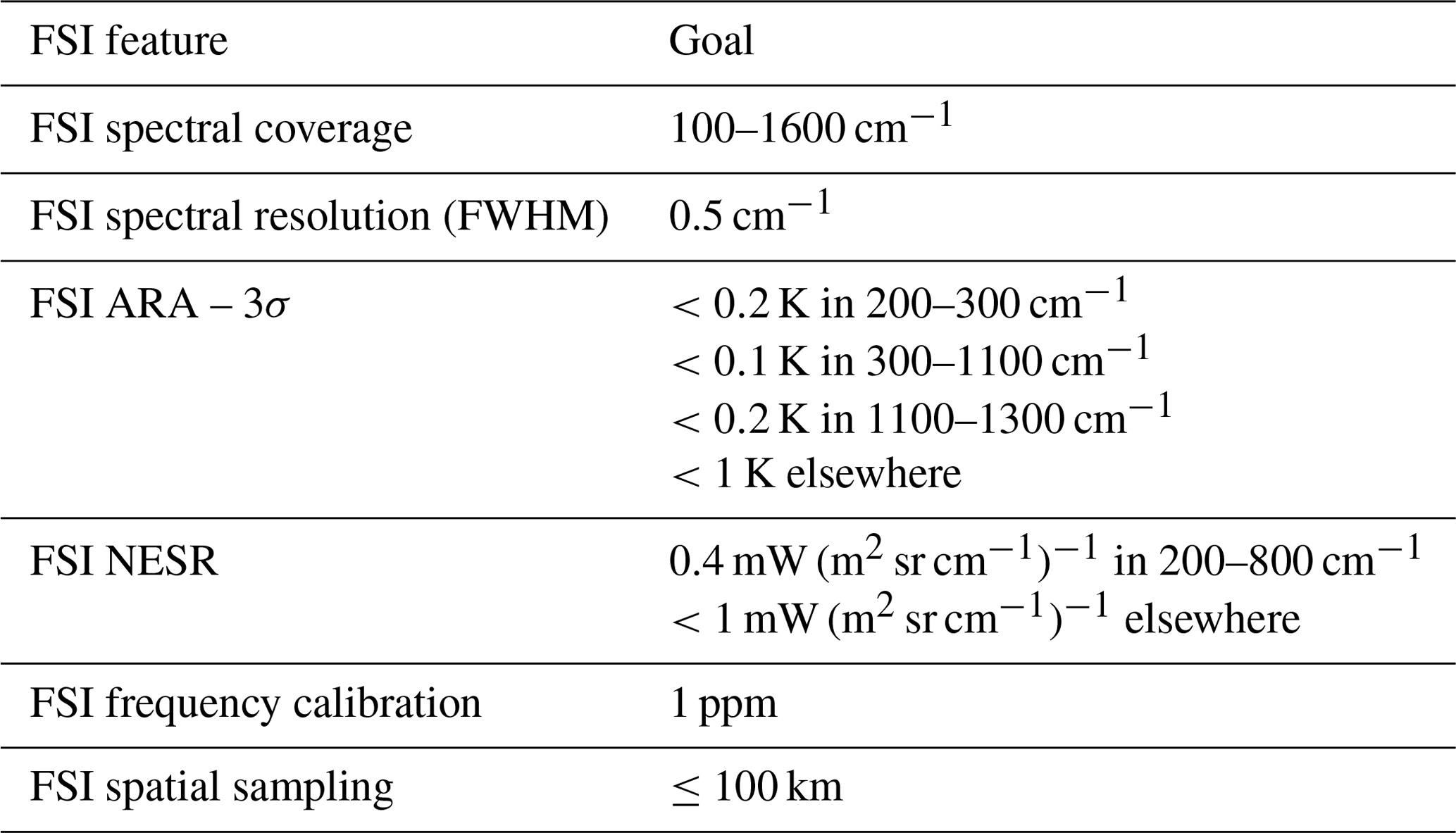
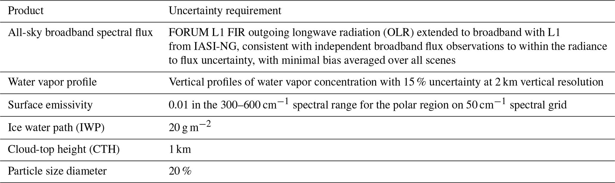
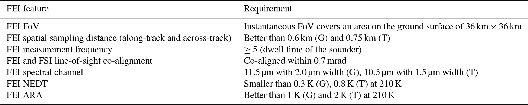
The requirements for the FORUM mission were defined from the scientific objectives of the mission in the framework of ESA project FORUMreq (see the FORUMreq final report available at https://www.forum-ee9.eu; last access: 21 January 2022). The complete sets of requirements for the FSI L1 (i.e., the calibrated and geolocated radiances), L2 (i.e., the retrieved geophysical quantities), and FEI L1 products are reported in Tables 1, 2, and 3, respectively. In this section, only the main specifications are discussed together with their driving scientific goals.
The FSI spectral range (100–1600 cm−1) was defined to cover most (95 % or more; ESA, 2019, p. 43) of the spectrum of the Earth's infrared emission to space, with a spectral resolution of 0.5 cm−1 to identify the spectral signatures due to seasonal, and interannual variations of water vapor in the upper troposphere – lower stratosphere (UTLS) range.
The requirements on precision were defined in terms of noise-equivalent spectral radiance (NESR) and were set to meet the primary research objectives of FORUM, namely to identify FIR features of water vapor, thin cirrus clouds, and surface properties.
One of the FORUM goals is to reduce uncertainty in climate predictions. The limits selected for absolute radiometric accuracy (ARA) allow us to capture typical climate feedback signals associated with changes in surface temperature or perturbations in water vapor. Importantly, the goal level of accuracy (0.1 K in 300–1100 cm−1) will also allow the observations to be used, with confidence, as a benchmark against which future spectrally resolved measurements can be compared (Wielicki et al., 2013).
Table 1FORUM FSI requirements. Note: FWHM is full width at half maximum.
Requirements on L2 products are realistically obtainable performances, which are derived by the instrument characteristics set by FSI requirements.
The area covered by the FEI field of view (FoV) is designed to include the FSI pixel (a circle of 7.5 km radius) and IASI-NG co-located measurements. A spatial sampling of 0.6 km is needed to detect clouds to which the FSI is sensitive (ESA, 2020; Dinelli et al., 2020).
Table 3FORUM FEI requirements. Note: NEDT is the noise-equivalent differential temperature; G is the goal (the optimal quality level that can be reached); T is the threshold (the minimum quality level that can be accepted).
2.3 The role of the E2ES
The key feature of the E2ES is the capability to introduce and single out possible causes for the discrepancies between the true and retrieved parameters. This applies to both the L1 products (i.e., the difference between the radiation reaching the instrument and the output spectrum) and the L2 products (i.e., the difference between the true atmospheric state and the atmospheric components retrieved by the inversion module).
The usual way of performing L2 simulations consists in using the same code for simulating the instrumental spectrum, adding some random error to the exact values, and then retrieving the atmospheric state. In other words, errors aside, all the simulated cases could be exactly retrieved by the inversion code. In the case of the E2ES, it is possible to simulate external factors, which must be definitively considered in the operative life of the instrument, and that can have an impact on the accuracy of the measurements. The main factors that can be simulated by the E2ES are as follows:
-
the instrument pointing errors,
-
the lack of homogeneity in the instrument field of view, and
-
the errors due to the instrument hardware that are not fully represented by the instrument spectral response function (ISRF), which acts as a convolution kernel on the simulated high-resolution radiances.
Unfortunately, there is often no sensitivity in the measurements to address such fine details. Nevertheless, we are able to quantify the degradation of the results due to these external factors.
The operative L2 products are also affected by the model error. The radiative transfer is performed via a code that emulates the main mechanisms governing the diffusion of the radiance in the atmosphere. Our Earth is, however, a much more complicated framework, and the most evident difference is that the atmosphere is a continuous system, while a discretization technique has to be applied anyway in order to be fed into a computer. However, this lack of knowledge cannot be attributed to the instrument, so adding a further uncertainty only interferes with the assessment of the instrument concept. Thus, the same forward model has been used in the generation of the scene and in the retrieval. In this way, we are sure that the radiative transfer does not introduce any bias with respect to the simulated observations.
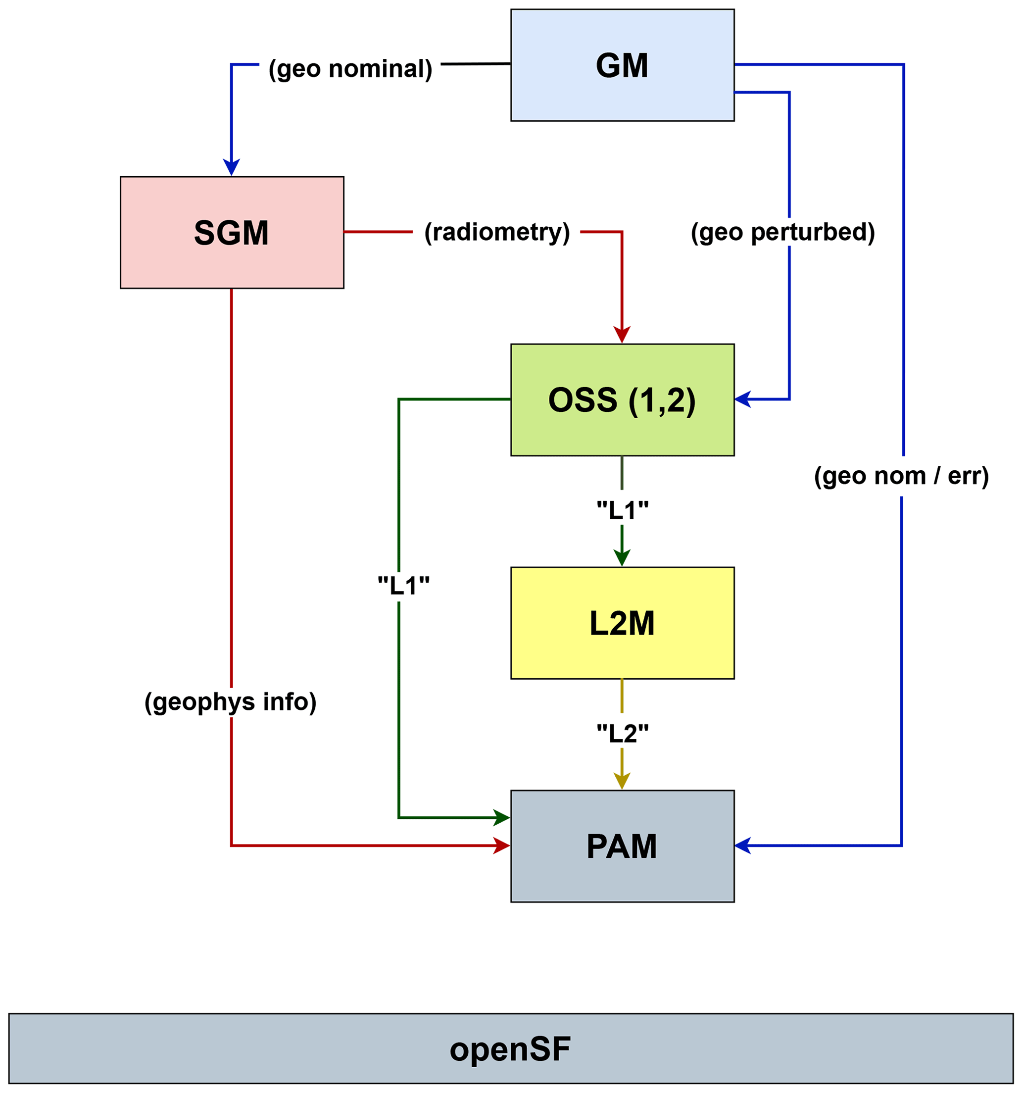
The E2ES is structured as a chain of modules that each perform a particular task. Each module relies on the data produced by the previous modules. The modules of the FORUM E2ES are as follows:
-
The Geometry Module (GM) calculates the true and error-affected geographical coordinates of the field of view based on satellite location and pointing.
-
The Scene Generator Module (SGM) calculates the high-resolution radiances reaching the instrument, using the exact geographical coordinates and the prescribed atmospheric parameters. This is considered to be the true state.
-
The Observing System Simulator (OSS) simulates the acquisition process of the instrument. Since in the preliminary phase, two different instrument concepts were available, two different configurations reproduce the two different hardwire instrument specifications.
-
The Level 2 Module (L2M) uses the spectrum generated by the OSS and the noisy geographical coordinates to retrieve atmospheric parameters.
-
The Performance Assessment Module (PAM) compares the true versus the retrieved L1 and L2 products and produces a report on the discrepancies.
The execution chain can be driven and checked from an external environment, the openSF structure, which is tailored for these kinds of simulators. Figure 1 represents the E2ES structure with the data flow.
In the following subsections, we briefly describe the purpose of the various modules and sketch the algorithms. The complete documentation may be found on the website devoted to FORUM, which is available at https://www.forum-ee9.eu/ (last access: 22 January 2022).
3.1 Geometry Module
The Geometry Module (GM) is a C executable in charge of providing the geolocation and observations angles for every sample of the FSI and FEI instruments. This requires computing the satellite orbit, the platform attitude, the instrument line of sight, and the intersection of this line with the Earth for every epoch and instrument sample.
The GM produces two types of instrument geolocation grids annotated with the sampling time and the observation angles: error-free grids (on top of which the SGM simulates the TOA spectrum) and estimated grids (intended to feed the OSS with a geolocation that is affected by telemetry and calibration uncertainties). The GM output files are written in netCDF format.
The GM configuration file, which is based on XML syntax, allows the user to define several simulation parameters, such as the latitude and longitude of the region of interest, the acquisition start and stop times, the satellite orbit and attitude (optionally also with knowledge errors), and the International Earth Rotation and Reference Systems Service (IERS) bulletin providing Earth rotation parameters, the focal length, the mirror scanning law, and the focal plane arrangement of FEI and FSI instruments and the spatial oversampling factor. The line of sight modeled with these parameters for every sample is then sent to the EO-CFI (Earth Observation CFI software; Sánchez-Nogales, 2020) to compute the geodetic coordinates of its intersection with WGS (World Geodetic System) 84 geoid or the selected digital elevation model.
3.2 Scene-Generator Module
The Scene-Generator Module (SGM) exploits the information on the geolocation and observational geometry provided by the GM and performs a simulation of gridded spectral radiances to feed the FORUM OSS. The SGM computes pixel-by-pixel radiances with the following three different approaches: a fully automatic setup, a user-driven scene definition, or a combination of the two methods.
In the automatic approach, multiple databases are loaded to configure the surface, atmosphere, and cloud properties in accordance with geolocation, season, and time of the day without any intervention from the user. For the storage limit, all the databases are currently available only for observations in the range 0–85∘ N and 0–30∘ E for two seasons (winter and summer) at four times of the day (00:00, 06:00, 12:00, and 18:00 UTC). The surface properties are described by the spectral emissivity, obtained from the geolocated emissivity database by Huang et al. (2016), and the skin surface temperature, obtained from the ERA5 reanalysis data (Hersbach et al., 2020). The atmospheric profiles of temperature, pressure, water vapor, and the other 11 gas mixing ratios, interpolated at fixed altitude levels, are derived from the ERA5 reanalysis and the IG2 climatological data (Remedios et al., 2007). The gases included in the simulation are H2O, CO2, O3, N2O, CO, CH4, O2, NO, SO2, NO2, NH3, and HNO3. Cross-section data using predefined values for the CCl4, CFC11, and CFC12 molecules were also added. The definition of the cloud geometrical and optical properties requires multiple steps. The ERA5 reanalysis provides the total cloud cover (cloud fraction within the pixel) and, for each vertical layer, the cloud liquid water and/or ice content (liquid water content and ice water content – LWC and IWC, respectively). It is assumed that liquid water and ice clouds can coexist in the same layer, even if they are computationally treated as two separate components. The LWC and IWC values are used to establish if the scene is clear or cloudy (total cloud cover) and for the definition of the cloud vertical structure. For each layer of the model, the liquid water particles effective radii (Re) are computed from the LWC by using the parameterization described in Martin et al. (1994), whereas the ice particle radii are derived from the IWC and the application of the parameterization by Sun and Rikus (1999) in its revised version by Sun (2001). The cloud optical depth (OD) at 900 cm−1 is derived, layer by layer, from information about the IWC (in the case of ice clouds) or LWC (in the case of liquid water clouds) and the effective radius of the particle size distributions (PSDs). The equation defining the OD at 900 cm−1 for vertically homogeneous clouds with the geometrical thickness of Δz is as follows:
where β(Reff,900) is the extinction coefficient at 900 cm−1 of the PSD corresponding to a specific effective radius, Reff, and normalized with respect to a unit IWC (or LWC for liquid water clouds).
Water clouds are simulated as the PSDs of liquid water spheres, while ice clouds are assumed to be composed of eight columns of aggregates crystals. Single scattering properties for single particles (SSSPs) are combined to compute the optical properties (extinction, scattering, and absorption coefficients and the phase function) for a set of PSDs over the whole FORUM spectral range. The assumed PSDs are modified gamma distributions (Hansen, 1971) representative of effective radii from 2 to 200 µm in the case of ice clouds and from 1 to 30 µm in the case of liquid water clouds. The SSSPs are derived from Yang et al. (2013) in the case of ice crystals and computed by using a Mie scattering code (Peña and Pal, 2009) when liquid water spherical particles are assumed.
Surface, atmosphere, and cloud properties are read and prepared as input for the LBLRTM (line-by-line radiative transfer model; Clough et al., 2005), for a clear-sky description. The cloudy-sky description, which includes multiple scattering, is prepared by using LBDLDIS (LBLrtm DISort; Turner et al., 2003), a code that uses the gas optical depth prepared by LBLRTM to build the input for DISORT (DIScrete Ordinate Radiate Transfer; Stamnes et al., 1988). DISORT is the code that calculates the multiple scattering due to the cloud. These radiative transfer routines compute the spectral radiances for the FORUM imager and sounder. The default output spectral resolution is set to 10−2 and 10−3 cm−1 for cloudy- and clear-sky simulations, respectively. The different resolution is adopted for the two cases as a compromise between computational speed and accuracy. In fact, for a resolution of 10−2 cm−1, the computational times in cloudy conditions decrease by a factor ranging from about 10 to about 20 with respect to using a 10−3 cm−1 resolution. Nevertheless, the simulation accuracy is maintained since FSI-OSS radiances in cloudy conditions computed using 10−2 or 10−3 cm−1 differ by less than the FSI goal NESR (figure not shown).
In the user-driven approach, the scene is manually configured, and the user is able to set a large set of input parameters to customize the specific simulation. Basically, all the parameters defining the surface and cloud properties are user configurable. Nevertheless, the vertical atmospheric profiles are automatically selected from the ERA5 or IG2 databases for the required geolocation and data, as in the automatic approach. However, the SGM configuration parameters include the list of the atmospheric gases used for the simulation, and thus, for each of them, their absorption properties can be turned off on request. The SGM allows the user to define surface temperature and emissivity, or to select specific emissivities from a list of 11 predefined surface types derived from Huang et al. (2016), including, e.g., water, desert, snow, and deciduous vegetation. In total, two different kinds of surfaces can be assumed to exist in the FORUM field of view. The shape of the areas covered by the different surfaces (with different emissivity and temperature) are defined by sectors or circles, whose sizes are set by the user through proper geometric parameters in the SGM configuration list. The scene can be assumed to be clear, overcast, or partially cloudy, adding a third or fourth level of possible heterogeneity to the observed scene. In this last case, the cloud covers only a fractional area of the full FORUM field of view, corresponding to a sector or a circle with configurable geometric features, such as in the case of the inhomogeneous surface scene. Liquid water, ice, or mixed-phase clouds can be placed at different top altitudes and be of any thickness – even overlapping each other when two clouds are assumed to be in the same scene (e.g., liquid–ice or ice–ice). In case of ice clouds at the moment, the user is allowed to choose between two ice particle shapes (column aggregates or hexagonal plates), for which the properties are derived from Yang et al. (2013), whereas the mixed-phase particles are considered to be spheres with an ice core and a liquid coating. The cloud optical properties are defined by selecting the particle size distribution effective radius and the total optical depth (at 900 cm−1). All of the configuration parameters are used to prepare the input files for the radiative transfer routines and to properly combine the output spectral radiances in the FORUM sounder representing the heterogeneity according to the chosen spatial oversampling.
Since the setting of the surface, atmospheric, and cloud properties are independent of each other, a mixed approach can be chosen by manually configuring some components and by letting the SGM configure the others.
Once the computations are performed for each pixel of the input grid (either being oversampled to the FSI footprint or not), the synthetic spectral radiances, the input configuration parameters, and other auxiliary information are passed to the OSS and PAM.
3.3 Observing System Simulator
Just as in the real instrument, the Observing System Simulator (OSS) is composed of two parallel modules that simulate the embedded imager and the Fourier interferometer.
3.3.1 FORUM Embedded Imager
The FORUM Embedded Imager Observing System Simulator (FEI-OSS) is a compiled MATLAB executable in charge of simulating and calibrating the instrument acquisition of the FEI thermal infrared imager. The FEI is modeled as an uncooled bolometer, with one spectral channel centered at 10.5 µm and a 2-D sensor layout of typically 60×60 pixels (configurable).
The FEI-OSS is composed of the instrument simulator (FEI-IS) and the L1b processor (FEI-L1).
The FEI-IS ingests the SGM output scene (possibly oversampled in the spatial domain), convolves the TOA spectra with the instrument point spread function (PSF) in the spatial domain, and integrates the resulting radiance with an instrumental spectral response function (ISRF) provided externally. Among its PSF modeling capabilities, the FEI-OSS is able to ingest an external PSF or to compute it by taking into account the configured parameters for the optics layout, the focal plane arrangement, the satellite motion blur, and other high-frequency contributions, such as the attitude and orbit control system (AOCS) jitter and the instrument microvibrations. Also, the channel center is configurable.
The FEI-L1 translates the instrument output radiance into calibrated spectral radiance by taking into account noise and other instrumental errors. In particular, the noise is simulated in the brightness temperature domain with a Gaussian distribution of a standard deviation equal to the configured noise-equivalent differential temperature (NEDT). The calibrated radiance is finally written into the L1b product (netCDF file), along with the estimated geolocation provided by the GM module and some flags related to the FEI/FSI co-registration.
3.3.2 FORUM Sounding Instrument
The FORUM Sounding Instrument Observing System Simulator (FSI-OSS) operates the software simulation of the performances of the FSI Fourier transform spectrometer from the starting point given by a set of input TOA spectral radiances provided by the Scene Generation Module (SGM). The simulator generates the interferograms corresponding to the outputs of the FSI instrument observing the selected scene, and then processes them with the L1 data analysis code in order to recreate the observed TOA radiance.
In order to account for the effects of the finite FoV of the FSI instrument and telescope, the input radiances are provided on a subpixel matrix which covers the FSI footprint plus a suitable safety margin and is needed to cover pointing errors in the simulations. Each of the subpixels is treated according to its specific observation geometry, i.e., specifically, its off-axis angle which produces a corresponding frequency shift due to the different pathlengths inside the FTS (Fourier transform spectrometer) and contributes accordingly to the output interferogram. This is the so-called self-apodization effect.
Also, to correctly model the acquisition during the instrument dwell time, several inputs are provided to the OSS, corresponding to different times in the duration of the acquisition. Each input will have, in general, different line-of-sight parameters, and the result of the processing of each of the inputs is interpolated at interferogram level in order to produce the complete interferogram acquired in the duration of the dwell time.
The reference optical design used in the FSI-OSS consists of a Mach–Zehnder interferometer, a design that provides the most general approach to a Fourier transform spectrometer. This design, in fact, allows us to place different sources on each of the two inputs of the interferometer and different detectors on each of the two outputs. It also allows the use of separate divider and recombiner beam splitters, which gives greater flexibility in the instrument design. Other optical schemes can be simulated as particular cases of this more general design.
The main configuration parameters that allow us to define the interferometer performances inside the FSI-OSS are the beam splitter reflection, transmission, and absorption coefficients, which are provided as complex, spectrally dependent quantities to obtain the most accurate and general instrument response modeling (Bianchini et al., 2009; Bianchini et al., 2019).
One of the inputs of the interferometer is permanently set on a black body source (reference black body – RBB), while the other can be switched between the scene and two other reference sources (cold black body and hot black body – CBB and HBB, respectively). This allows us to operate the FSI-OSS in two different modes, scene and calibration, in order to simulate the full measurement process of the FSI instrument.
To obtain a meaningful representation of the interferogram that is observed on the outputs of the FSI, the OSS needs to define a further set of transfer functions that describe the behavior of the optical and electronic components of the system.
An overall frequency-dependent absorption coefficient can be defined in order to model possible effects due to optical components. Moreover, transfer functions describing the electronics response, expressed in terms of phase and amplitude, are applied in order to correctly represent the output interferograms. The electronic response function can be further subdivided into detector response and preamplifier response, if needed. A last transfer function is used to model the effects of sampling and digitization, with the possibility of introducing arbitrary random or periodic sampling errors or a calibration error in the interferogram timescale.
All of the above-described functions are coded in the instrument module, which outputs the simulated interferograms. The L1 module has the function of transforming and calibrating the interferograms in order to reconstruct the observed scene radiance (Bianchini and Palchetti, 2008). The L1 module is subdivided into the following three parts:
-
Level 1a, which performs the Fourier transform of the interferogram, including the possible application of compensations for the different instrumental transfer functions, the zero path difference detection, and the phase correction of the interferogram, producing, as output, the uncalibrated spectrum.
-
Level 1b, which performs the radiometric calibration of the uncalibrated spectrum and the estimation of the a priori errors deriving from the calibration procedure (calibration error) and the detector noise (NESR error), providing, as output, the measured atmospheric spectral radiance corresponding to the input scene, as observed on each of the two instrument outputs.
-
Level 1c, which performs the averaging of the two instrument outputs and the resampling of the average spectrum on a configurable frequency scale, in order to provide the L2 module with a single measured spectrum with the required spectral sampling. The resampling is done through fast Fourier transform (FFT) interpolation and zero padding in case of oversampling.
The frequency scale is chosen to obtain statistically independent adjacent measures. This leads to a diagonal variance–covariance matrix (VCM) with respect to the NESR component, which is the dominant one. The resolutions obtained are 0.35714 and 0.37037 cm−1 for the two instrument concepts.
Last, a separate FSI-OSS module is used to calculate the ISRF corresponding to the configured FSI optical setup. This module performs the calculation of the ISRF, taking into account the effect of the finite maximum optical path difference and the line broadening and shift due to the finite divergence of the radiation propagating inside of the interferometer (the self-apodization effect). The ISRF module generates an output file in a format which is directly compatible with the L2 module.
3.4 Level 2 module
The Level 2 module (L2M) is composed of the L2M_CIC (cloud identification and classification) and L2M_I (inversion) submodules. A Python wrapper gathers the input data and runs the two submodules, providing the correct configuration files.
3.4.1 Cloud identification and classification
The main goal of the L2M_CIC submodule is to provide a classification of the observed spectrum. A machine learning algorithm named CIC (Maestri et al., 2019b) is embedded in the L2M_CIC routine and used to classify the FORUM sounder input spectrum. In total, the following four different predefined classes are used: clear sky, liquid water cloud, optically thick ice cloud, and cirrus cloud. The classification is based on the comparison of the input spectrum with four training sets (TSs) containing the precomputed spectra of the four classes. A principal component analysis determines the level of similarity of the input spectrum to the elements of each TS and selects the class of pertinence. If the spectrum is classified as cloudy (liquid water, thick ice cloud, or cirrus cloud) key cloud parameters are derived and passed to the inversion module as initial conditions. The cloud parameters are cloud top height, thickness, particle effective radius, and optical depth at 900 cm−1. Their values are derived from climatological data of cloud properties (cloud Climate Change Initiative, CCI, see Stengel et al., 2017; cirrus clouds, see Veglio and Maestri, 2011) and atmospheric profiles (ERA5; Hersbach et al., 2020), according to the cloud classification and the geolocation, season, and observed brightness temperature at 900 cm−1.
The CIC algorithm classification is based only on FORUM sounder spectral radiance and, thus, regards the radiance from an extended (about 15 km diameter) field of view. The classification is provided independently of the presence (or not) of subpixel heterogeneities. Therefore, a scene classified as cloudy could be the result of a field of view that is only partially covered by clouds plus a clear-sky fractional area and vice versa. The L2M_CIC exploits the FORUM imager data to pair the spectrum classification with a scene homogeneity information. The imager pixels radiances are first converted into brightness temperatures (BTs), and then a BT distribution (histogram) is analyzed with a custom made fitting function. A simple algorithm identifies the BT distribution modes and splits the imager pixels into homogeneous groups of pixels characterized by limited BT variation. Thus, the L2M_CIC submodule provides auxiliary information concerning the number of homogeneous areas identified at FORUM sounder subpixel level, their average BT, and standard deviation. This is used as a quality flag for the inversion results, since nonhomogeneous scenes are, in any case, managed as homogeneous in the retrieval process. A land mask for the imager field of view is also defined, based on the Global Self-consistent, Hierarchical, High-resolution Geography Database (GSHHG; Wessel and Smith, 1996, and updates), so that the BT inhomogeneities caused by different sea or land surfaces are easily identified, especially in clear-sky conditions.
3.4.2 Inversion
The purpose of the inversion module is to solve the inverse radiative transfer problem by retrieving any combination of surface temperature, surface emissivity, and vertical profiles of temperature and water vapor in clear-sky conditions and cloud parameters in cloudy-sky conditions. The retrieval algorithm is based on the classical OE (optimal estimation) method (Rodgers, 2000). The inversion is performed via the Gauss–Newton sequence, with the Marquardt modification to ease the Hessian inversion and to compensate for the nonlinearity of the forward model. The a posteriori IVS (iterative variable strength) regularization technique (Ridolfi and Sgheri, 2011; Eremenko et al., 2019; Sgheri et al., 2020) is then applied to smooth out the retrieved profiles. In accordance with the SGM, the code makes use of the LBLRTM forward model in clear-sky conditions and the LBLDIS frontend to the DISORT (Discrete Ordinates Radiative Transfer Program for a Multi-Layered Plane-Parallel Medium) multiple scattering code in cloudy-sky conditions. In cloudy-sky conditions, when a cirrus cloud is detected, the inversion module includes a preprocessor that, using the parameter decoupling technique, finds a better estimate for the cloud parameters than the CIC guess. This feature is important to avoid the retrieval stopping on local minima (see the discussion of the cloudy tests for more explanations). We used the fDISORT (fast DISORT), an accelerated version of DISORT (Sgheri and Castelli, 2018), which is able to reduce the multiple scattering computation time. The instrumental effects are factored via the convolution with the ISRF function. In this early version of the FORUM E2ES, the decision was made to maintain a frequency-dependent ISRF. Consequently, the convolution cannot be computed in the Fourier domain. We obtained the actual ISRF on a rather fine grid, with sampling step of 3 cm−1. However, using the apodized sampled ISRF can increase the chi-square by up to 30 %, with respect to the unapodized spectrum, due to the fact that we exchange the interpolation and apodization operators. The correct sequence of first convolving with the sampled ISRF and then convolving with the apodization kernel increases the computation time and does not remove the error introduced by cutting the tails of the ISRF, which is one of the purposes of apodization. Thus, at least in this stage, we preferred to use the unapodized spectrum.
3.5 Performance Assessment Module
The Performance Assessment Module (PAM) is a MATLAB executable that aims to compute and plot the retrieval accuracy of L2M. In particular, this module also allows the inspection of the SGM output (TOA spectral radiance) and plotting the L2M vs. SGM profiles, including error bars and residual statistics for clear-sky retrievals (emissivity, skin temperature, atmospheric temperature, atmospheric water vapor, and precipitable water vapor) and cloudy-sky retrievals (cloud-top height, cloud optical depth, cloud particle size, cloud thickness, and ice/liquid water path). The PAM is also able to plot the averaging kernel (AK) profiles calculated by the L2M and the vertical resolution, which is computed at each level as the full width at half height (Rodgers, 2000) of the corresponding AK row. Averaging kernels may be optionally convolved with the SGM reference for comparison to the L2M retrievals.
The FORUM E2ES (FEES) is meant to study the potentialities and criticalities of the FORUM mission for realistic characteristics of the instrument and for different measurement scenarios.
The different measurement scenarios, used both for the validation of the different modules and the assessment tests, were defined in the homogeneous case to be representative of seasons and latitudes in clear and cloudy conditions.
The FEES is able to simulate FORUM measurements all over the globe, provided that the climatological data are included in the SGM dataset (see the relevant section).
Within the area selected for the FORUM E2ES study, the following seven scenarios were identified: three extreme cases (two in polar regions in winter with two different surface characteristics, ice and fine snow, and one in the tropics on the desert) and four cases at the middle latitude (two on the sea in summer and two on vegetation, with one in summer and one in winter). These scenes can be simulated in either a clear sky or cloudy sky.
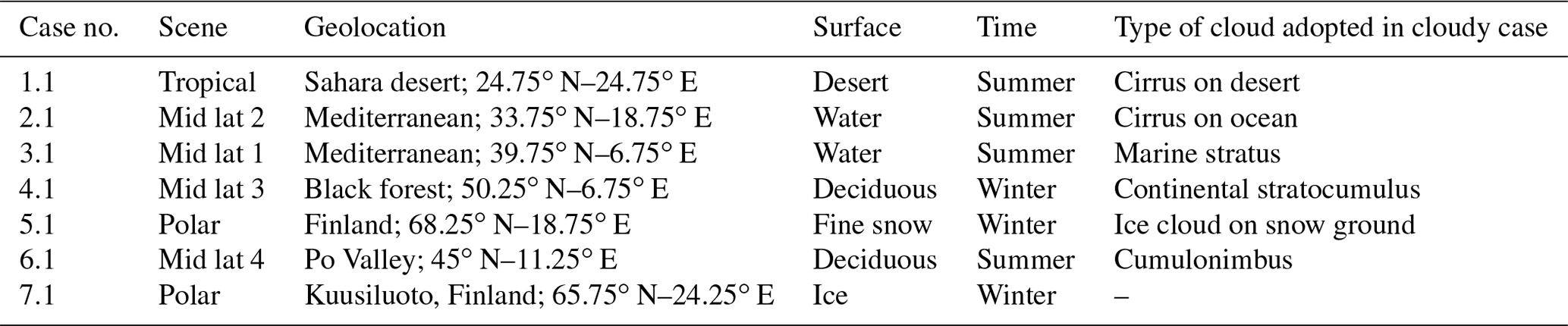
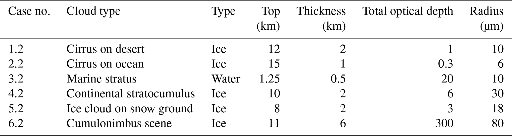
Table 4 provides, for each scene, the geolocation, type of surface, and time, as well as the type of cloud assumed for each scene in the case of cloudy sky. The cloudy-sky scenarios are computed, adding different homogeneous types of clouds to the clear-sky atmosphere and filling all the FoV (see Table 5).
Table 5Cloud characteristics associated to the scenes considered.
We depart from real data when using this approximation; however, it does not have an impact on the assessment of the performances of the E2ES.
In the assessment tests, we also used the capability of SGM to simulate heterogeneous scenes by assuming a FoV covered by portions of different homogeneous atmospheres.
Assessment tests were performed to evaluate the quality of the L2 products, assuming the FORUM instruments were in a configuration satisfying the L1 goal requirements, for the different scenarios identified to cover a variety of atmospheric characteristics. These tests were performed for both homogeneous and inhomogeneous scenes in both clear-sky and cloudy-sky conditions.
The results obtained in the homogeneous case represent the best that can be obtained from FORUM for the different scenes; hence, the quality of the products obtained in these conditions constitutes the reference for the other tests performed with heterogeneous scenes.
The L2 clear-sky products of the E2ES were also validated by comparing them with the outputs obtained, starting from the same observations generated by the FSI module by an already validated correlative code. The reference code used in clear sky is KLIMA (Kyoto protocoL Informed Management of the Adaptation).
Conversely, the L2 cloudy-sky products of the E2ES were compared with the outputs of the reference SACR (Simultaneous Atmospheric and Cloud Retrieval) code. However, due to some differences in the model and approach, we cannot speak rigorously of a validation.
5.1 Homogeneous clear-sky cases
The seven clear-sky test cases listed in Table 4 were analyzed. The simulated observed spectra were generated by the E2ES chain, including the GM, the SGM, the FEI, and the FSI. The reference atmospheric state was constructed using ECMWF information. The vertical grid used to represent the atmospheric profiles in both the SGM and the L2M is composed of levels that are about 0.5 up to 15 km, 1 km (from 15 to 25 km), 5 km (from 25 to 40 km), and 10 up to 80 km. In the retrieval, we also tested an optimized grid similar to that of Ridolfi et al. (2020). However, in the E2ES retrieval setting, we obtained worse results because a coarser grid introduces a smoothing error, which is particularly noticeable in the tropospheric water vapor profiles. The used noise error and spectral resolution are aligned with information provided by the industrial consortia and compliant with the goal parameters specified in Tables 1 and 3. Temperature, water vapor, surface temperature, and surface emissivity are retrieved simultaneously by L2M using the optimal estimation approach. The covariance matrices of the a priori vertical profiles of temperature and water vapor are built assuming the errors defined by the UK Met Office for routine assimilation of IASI products into their operational numerical weather prediction (NWP) system (see Fig. 6). Indeed, IASI-NG measurements are planned to be used in synergy with the FORUM measurements. For the emissivity, which is represented on a 5 cm−1 spaced grid, we used a constant error of 0.05, with a correlation length in the wavenumber of 50. For surface temperature, an a priori error of 2 K was used. The a priori profiles used for these tests for all the retrieved variables are given by the truth perturbed with 1 standard deviation of the a priori error. This is the most sensible choice, especially for emissivity. In fact, the sensitivity to the emissivity in the spectrum is different in different regions of the spectrum. If a stochastic perturbation were used, then the results would depend on how large the actual perturbation is in the frequency ranges where there is sensitivity. For the initial condition of the retrieval, we used, for temperature, water vapor, and surface temperature, the values taken from the climatology, obtained as the 10-year local average in the month of ECMWF analysis profiles, while the a priori values were used for emissivity. The reason for this difference is that the Gauss–Newton (GN) method only looks for local minima. Starting from the a priori, the chance to obtain a solution close to the a priori itself is not negligible. On the other hand, the dependence of the spectrum from emissivity is linear, so the possibility of finding a local minimum for the emissivity itself is minimal. However, the combined retrieval of emissivity and surface temperature raises an issue that is discussed in this paper.
5.1.1 Validation with KLIMA code
The KLIMA code, used to validate the L2M module in clear-sky conditions, performs the retrieval of the atmospheric profiles and surface parameters from the spectral radiance measurements. The code consists of two distinct modules, namely the forward model (FM) and the retrieval model (RM). The RM has been developed in the context of the KLIMA ESA study (Cortesi et al., 2014) by upgrading the algorithm employed for the analysis of REFIR-PAD measurements (Bianchini et al., 2008), which was adapted, in turn, from the MARC (Millimetre-wave Atmospheric Retrieval Code) inversion code for the MARSCHALS ESA (European Space Agency) study (Carli et al., 2007). The FM is a line-by-line radiative transfer model, with capability to simulate wideband spectral radiances based on the following key features: radiative transfer calculations performed using the Curtis–Godson approximation, atmospheric line shapes modeled with the Voigt profile, and an atmospheric continuum model, taking into account the main contributions from N2, O2, O3, H2O, and CO2. To be consistent with L2M_I, the spectroscopic database adopted for the simulations is AER (Atmospheric and Environmental Research) version aer_v_3.7 (http://rtweb.aer.com/line_param_frame.html; last access: 22 January 2022). The atmospheric continuum is modeled using the routine MT_CKD_3.3 (http://rtweb.aer.com/continuum_whats_new.html; last access: 22 January 2022), considering the contribution of the lines external to the region of ±25 cm−1 from the line center. A dedicated spectroscopic database and line shape are adopted for CO2 to take into account the line mixing effect when using the AER spectroscopic database (http://rtweb.aer.com/line_param_frame.html; last access: 22 January 2022). Moreover, the correction of the Planck function (Clough et al., 1992) is included to take into account the optical depth of the atmospheric layer at the different frequencies. The only difference between the KLIMA and LBLRTM forward models is in the line-shape; KLIMA uses the Voigt function, while LBLRTM uses a linear combination of faster functions, thus performing a grouping of nearby lines. The validation of KLIMA FM was conducted in the context of IASI data analysis (Cortesi et al., 2014) by comparing synthetic IASI measurements generated by the KLIMA FM code with those of the FM of the LBLRTM. The RM uses a constrained nonlinear least squares fitting approach and the cost function to be minimized, taking into account the a priori information (optimal estimation method) and the Marquardt parameter. The code implements the multi-target retrieval, where more than one species is simultaneously retrieved along with many other atmospheric, surface, and instrumental parameters. A complete covariance matrix (CM) can be used, including both the measurement errors and the errors in the calibration procedure and/or in the estimation of the FM parameters.
The purpose of the validation was to compare the retrieved quantities and the corresponding errors (given by the mapping of measurement error on retrieved quantities) provided by the L2M_I of the E2ES and by KLIMA when starting from the same conditions. The validation may be considered as having been reached if the differences in the estimated retrieval error and the differences in the retrieved profiles are small enough. More precisely, we set a goal at 10 % of the retrieval error for the retrieved profiles. Moreover, we ask for the difference in the retrieval error to be less than 10 %. With the actual results, statistically, these goals are achieved.
In Table 6, we report on the comparison between the initial and final reduced χ2 (chi-squared) obtained using KLIMA end L2M_I. The number of Gauss iterations is also reported. Each row of Table 6 refers to a different scenario. The reduced χ2 differences (both initial and final) are smaller than 0.02. Although the convergence criteria are the same (i.e., reduction in the χ2 is less than 1 %), the number of Gauss iterations in some cases is different. This is due to differences in reduced χ2 of the order of 0.001.
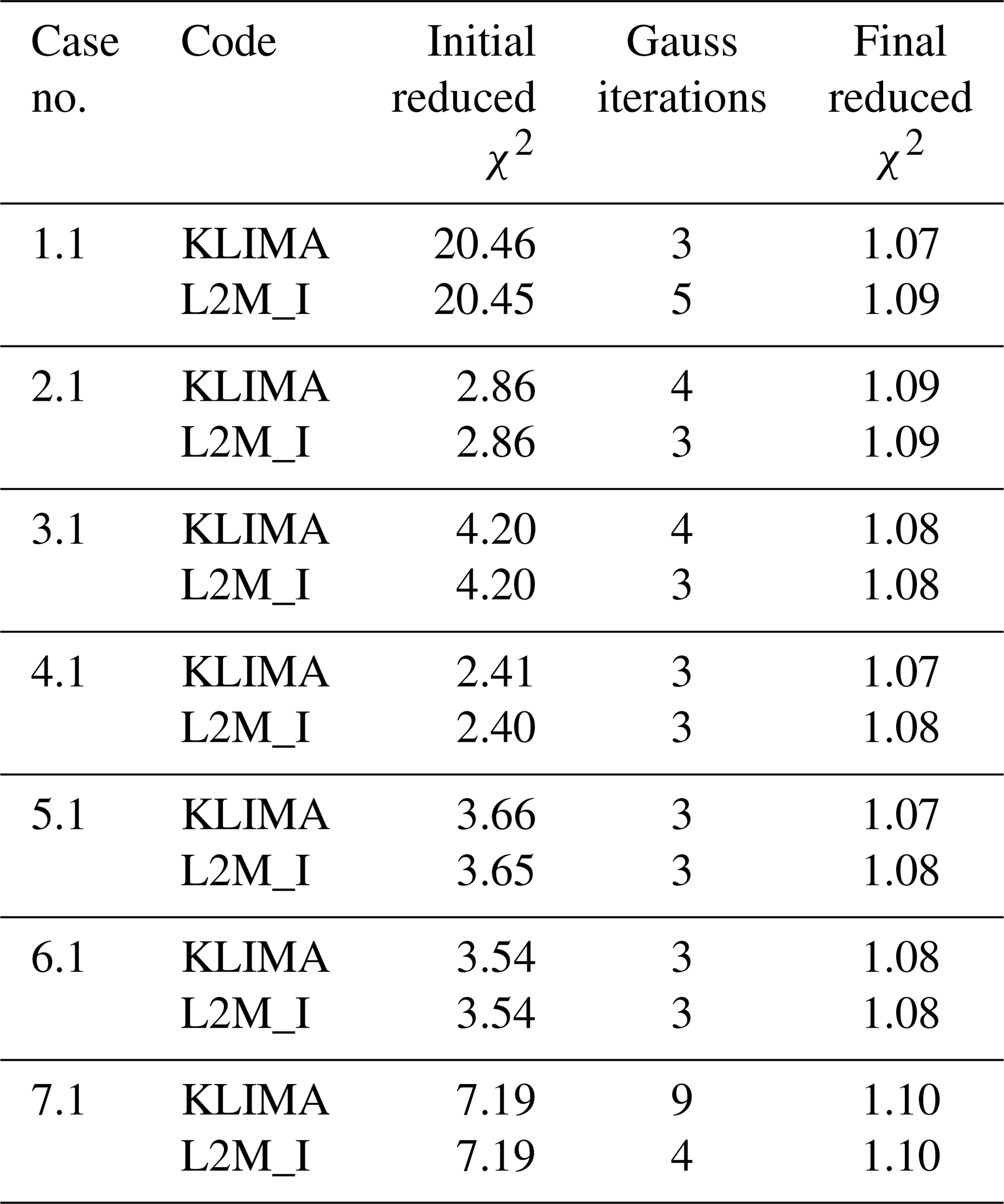

Figure 2(a) Difference in the water vapor profile obtained from KLIMA and L2M_I divided by the mean value of the retrieval error for the seven analyzed scenarios. (b) Difference in the water vapor retrieval error profile obtained from KLIMA and L2M_I divided by the mean value of the retrieval error for the seven analyzed scenarios.
In Fig. 2, we report on the comparison between the retrieved H2O value profile and error profile obtained when using KLIMA and L2M_I. The differences are divided by the mean retrieval error. The differences between the retrieval errors are smaller than 5 %, and the differences between the profiles retrieved by the two codes are smaller than 0.4 times the retrieval error, with the maximal difference concentrated in the lower tropospheric region.
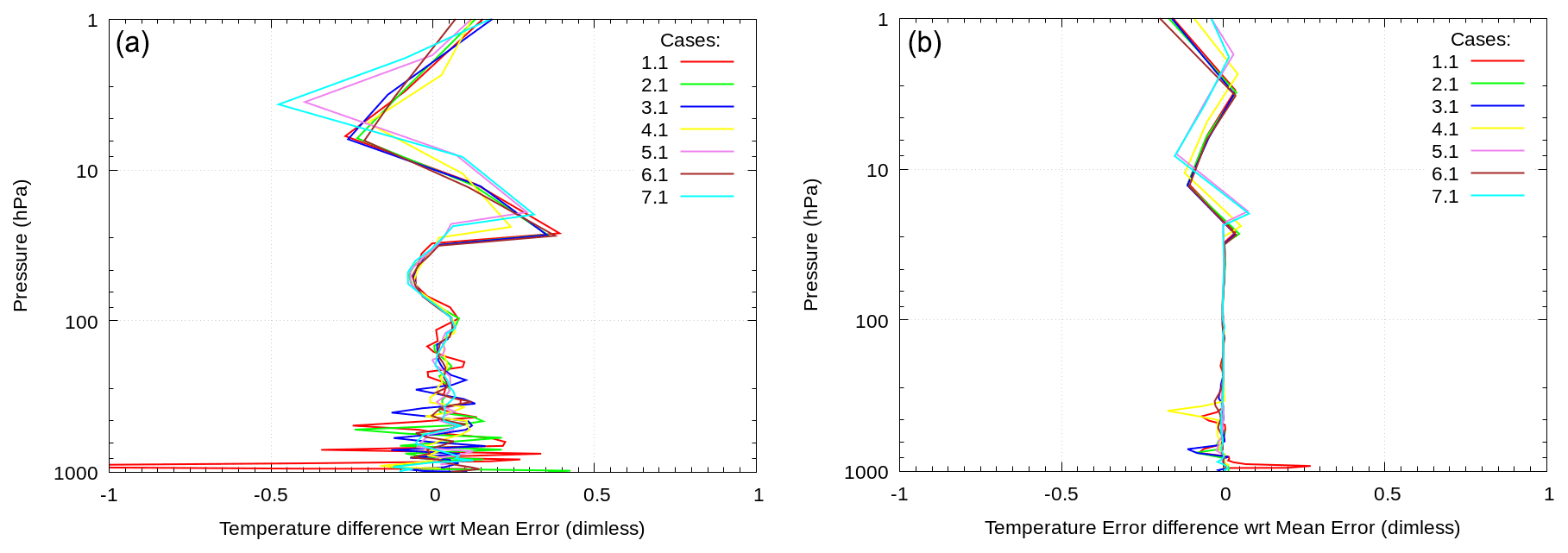
Figure 3(a) Difference in the temperature profile obtained from KLIMA and L2M_I divided by the mean value of the retrieval error for the seven analyzed scenarios. (b) Difference in the temperature retrieval error profile obtained from KLIMA and L2M_I divided by the mean value of the retrieval error for the seven analyzed scenarios.
The results for temperature validation are reported in Fig. 3. The differences between retrieval errors are smaller than 25 %, and the differences between the profiles retrieved by the two codes are mostly smaller than 0.5 times the retrieval error.

In Table 7, we report on the comparison between the retrieved surface temperature and error obtained using KLIMA and L2M_I. Each row of Table 7 refers to a different scenario. The differences between the retrieval errors are smaller than 15 %, and the differences between the profiles retrieved by the two codes are mostly smaller than 0.3 times the retrieval error.
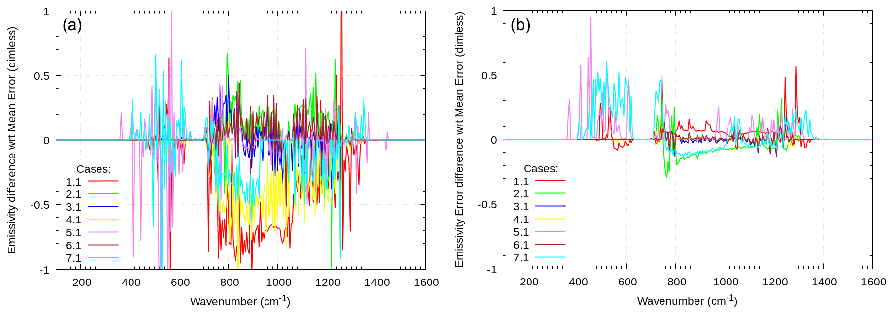
Figure 4(a) Difference in the surface emissivity spectrum obtained from KLIMA and L2M_I divided by the mean value of the retrieval error for the seven analyzed scenarios. (b) Difference in the surface emissivity retrieval error spectrum obtained from KLIMA and L2M_I divided by the mean value of the retrieval error for the seven analyzed scenarios.
In Fig. 4, we report on the comparison between the spectrum of the retrieved surface emissivity and its error spectrum obtained using KLIMA and L2M_I. The differences are divided by the mean retrieval error. The differences between the retrieval errors are smaller than 30 %, and the differences between the profiles retrieved by the two codes are mostly smaller than 0.5 times the retrieval error. The larger differences in the MIR range that show up in some cases are mainly due to the high negative correlation between surface temperature and emissivity. For the retrieval procedure, the effect of a lower surface temperature with a higher emissivity is similar to that of a higher surface temperature with a lower emissivity.
5.1.2 Discussion of the results
We describe a selection of the results here.
In Fig. 5, we report on the simulated spectra and the residuals (given by the difference between simulated observations generated by the OSS and the best-fit L2 simulated radiances) for the seven clear cases. The different cases are characterized by large differences in both the FIR and the MIR spectrum. However, in all cases, the residuals are compatible with the measurement noise and show no bias. In Fig. 6, we report on the retrieved profiles, the retrieval errors (estimated from the diagonal elements of the CM), and the differences between the retrieved and the true profiles of temperature and water vapor for all the seven cases.
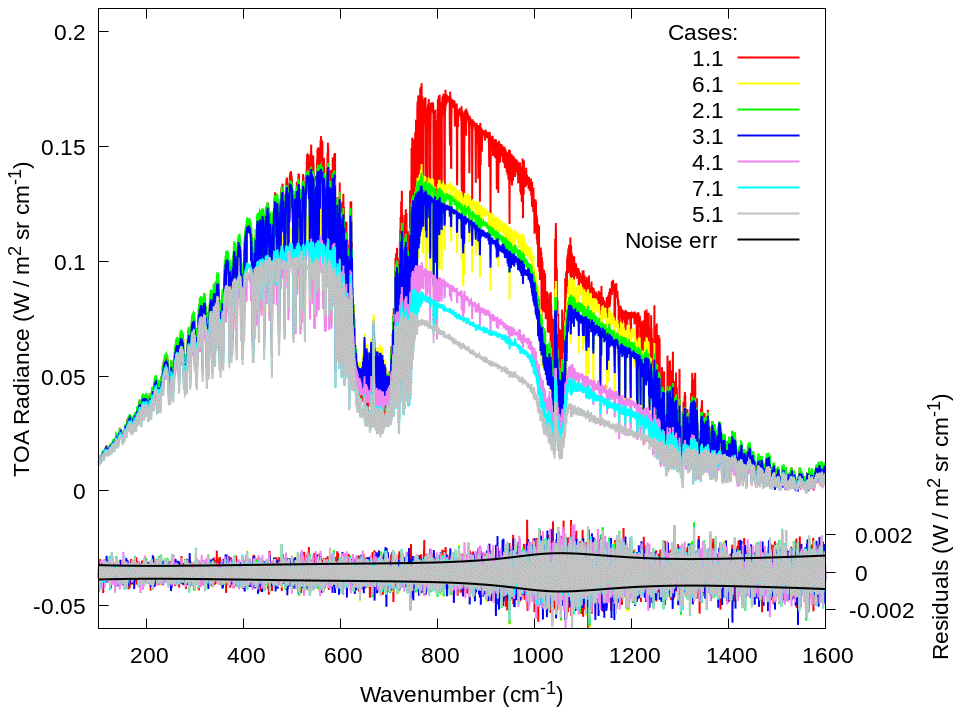
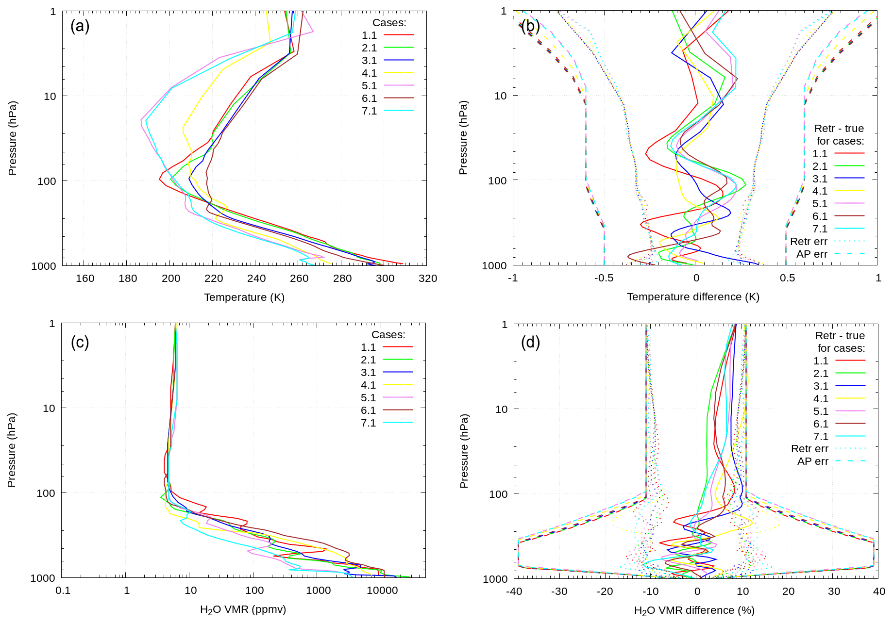
Figure 6Retrieved temperature profiles for the seven clear-sky cases (a). Difference between retrieved and true temperature profiles, with the retrieval and a priori error shown (b). Retrieved water vapor profiles for the seven clear-sky cases (b). Difference between retrieved and true water vapor profiles, with the retrieval and a priori error shown (d).
For both temperature and water vapor, the difference between the retrieved profile and the truth is well within the retrieval error for most of the points and all cases. Despite the variability in the temperature and water vapor profiles in the various cases, the sensitivity of the temperature and water vapor retrieval, given by the retrieval error, does not change significantly, and the requirements on precision are met in all cases. The information gain quantifier (IGQ; Dinelli et al., 2009) is defined as being 2 times the base 2 logarithm of the ratio between the a priori error and the retrieval error, and it measures the contribution of the measurements in the retrieved values. The IGQ is larger than 2 for temperature and larger than 4 for water vapor in troposphere. In Fig. 7, we report on the typical behavior of the AKs for temperature and water vapor. The values of the diagonal elements significantly smaller than 1 in the troposphere do not depend only on the fact that the used a priori errors are small and, hence, the information gain is limited. This is also the case on the very fine retrieval grid used in the troposphere which determines the small information content in each retrieved component. The most useful information in this case is provided by the number of degrees of freedom (DOF), which is given by the trace of the averaging kernel matrix. The DOF of the temperature profile varies from 7 for case 1.1 (tropical dry case) and about 6 for case 2.1 (middle latitude case) to 5 for case 5.1 (polar case), with 75 % of the DOF being concentrated in the lowest 25 km. For the water vapor profile, the number of DOF varies from 8.2 for case 1.1 and 7 for case 2.1 to 5.4 for case 5.1, with more than 90 % of DOF being concentrated in the lowest 25 km.

Figure 7Averaging kernels for temperature (a) and water vapor (b) for case 1.1 (clear-sky desert at noon in summer).
Table 8 reports on the results of the surface temperature retrieval. All cases show a good accuracy, with an IGQ larger than 4. The exception is case 1.1 (desert at noon in summer), where there is a negative bias of 0.8∘ which is larger than the retrieval error. This is due to a large negative correlation between the surface temperature and emissivity in the MIR. This is further discussed when dealing with the results for surface emissivity.
Table 8Results for the retrieval of surface temperature for the seven clear-sky cases.
For emissivity retrieval, we can divide our sample into the following three groups with similar atmospheric conditions:
-
polar cases (5.1 and 7.1), i.e., high latitude and dry atmosphere (snow and ice),
-
middle latitude cases (2.1, 3.1, 4.1, 6.1), i.e., water vapor rich atmosphere over water or deciduous ground, and
-
the desert case (1.1), which combines a dry atmosphere and hot surface temperature. Also, the emissivity pattern has substantial features in the MIR region and the quartz Reststrahlen bands (Salisbury and D'Aria, 1992), which are also called the devil's horns.
Table 9Emissivity retrieval DOF for the three model cases. FIR limit is placed at 666 cm−1. The retrieval grid is fixed, and 301 emissivity points are retrieved, with 114 belonging to the FIR and 187 to the MIR, respectively.
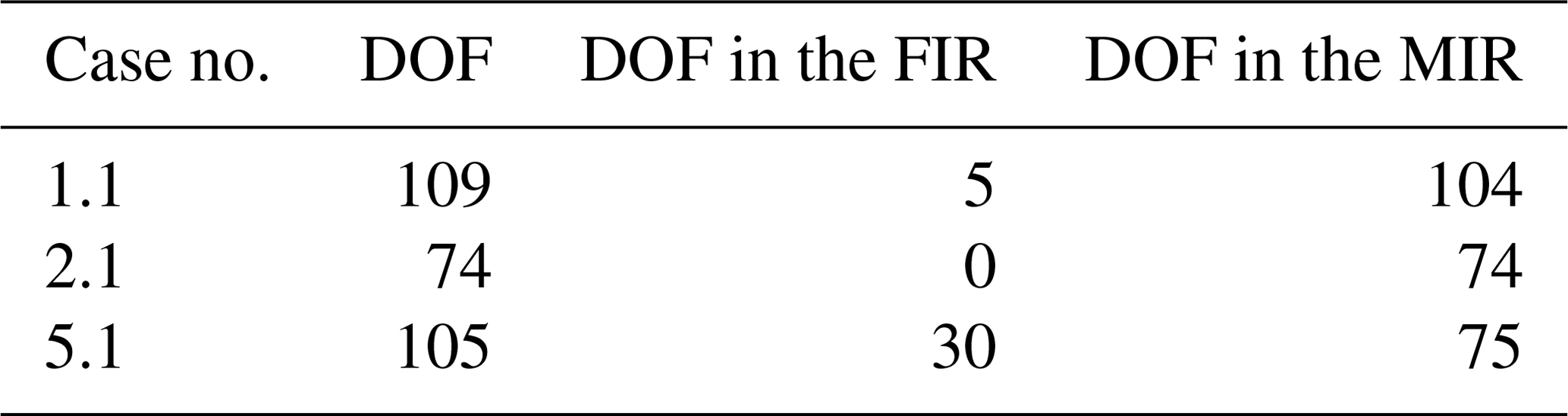
We selected one model case from each group. The number of DOF is reported in Table 9 for the FIR and MIR regions. These numbers are directly comparable because the emissivity grid is the same for all cases.

Figure 8Emissivity retrieval for case 5.1 (polar case on fine snow). (a) A priori profile with error bars (green), retrieved profile with error bars (red), and truth (blue). (b) Difference between retrieved and true (red) and the retrieval error (blue), together with the difference between a priori and model (green) and a priori error (cyan).
For the polar group, we show case 5.1 in Fig. 8. We note that, as expected due to the dry atmosphere which makes it transparent to the surface also in the FIR, there is sensitivity to the measurements in both the FIR and MIR regions.
This emerges also from the analysis of the AKs of the frequency-dependent emissivity profile (see Fig. 9) characterized by values of the diagonal matrices very close to 1 in the 500–600 cm−1 and in the 700–1000 cm−1 regions. In these regions, the a priori information contributes only very marginally to the inversion, and the grid is sufficiently coarse to allow each component of the used frequency grid to capture significant information.
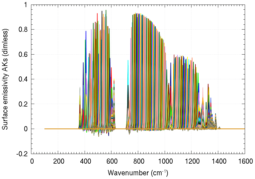
Figure 9Averaging kernels of the frequency-dependent emissivity profile for case 5.1 (polar case on fine snow).
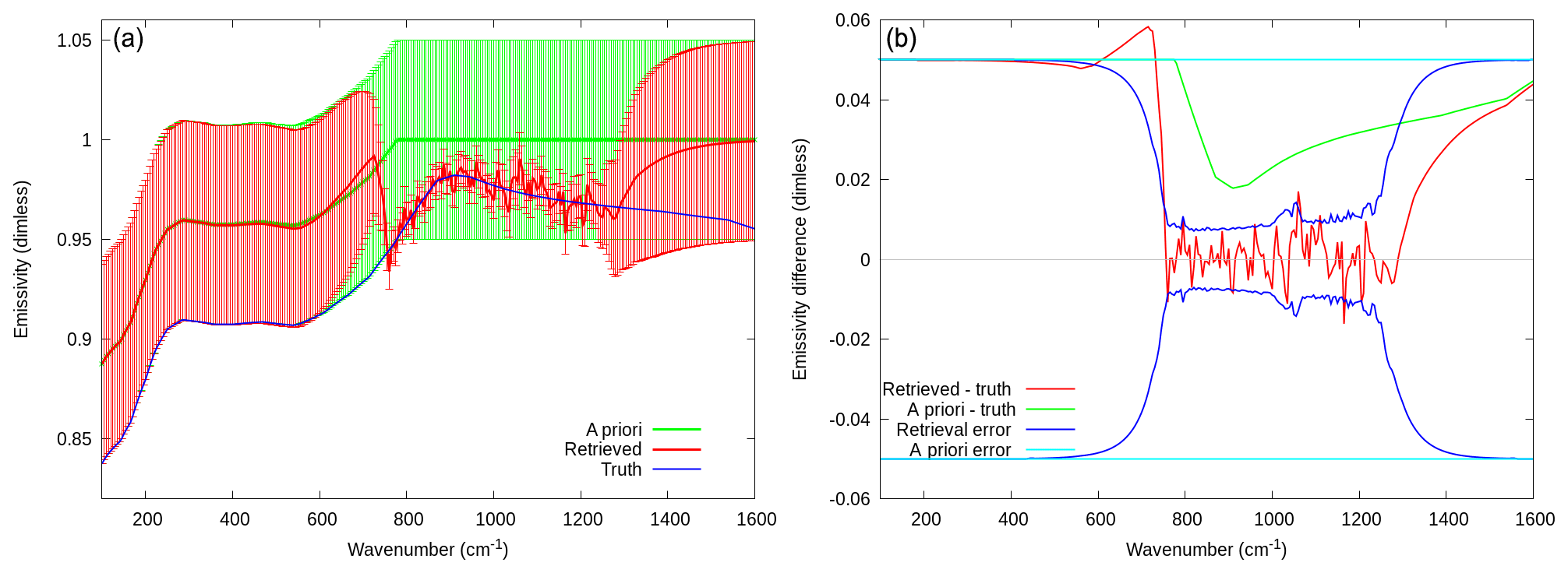
Figure 10Emissivity retrieval for case 2.1 (middle latitude on water). (a) A priori profile with error bars (green), retrieved profile with error bars (red), and truth (blue). (b) Difference between retrieved and true (red) and the retrieval error (blue), together with the difference between a priori and model (green) and a priori error (cyan).
For the middle latitude group, we show case 2.1 in Fig. 10. In these cases, the rich water content in the troposphere masks the emissivity signal in the FIR, so there is only sensitivity in the MIR atmospheric window where the transparency of the atmosphere allows us to obtain information on the surface.

Figure 11Emissivity retrieval for case 1.1 (desert at noon in summer). (a) A priori profile with error bars (green), retrieved profile with error bars (red), and truth (blue). (b) Difference between retrieved and true (red) an retrieval error (blue), together with the difference between a priori and model (green) and a priori error (cyan).
Finally, in case 1.1, the retrieval of the emissivity shows some sensitivity in the FIR region but also a positive bias of about 0.01 in the MIR region, as shown in Fig. 11.
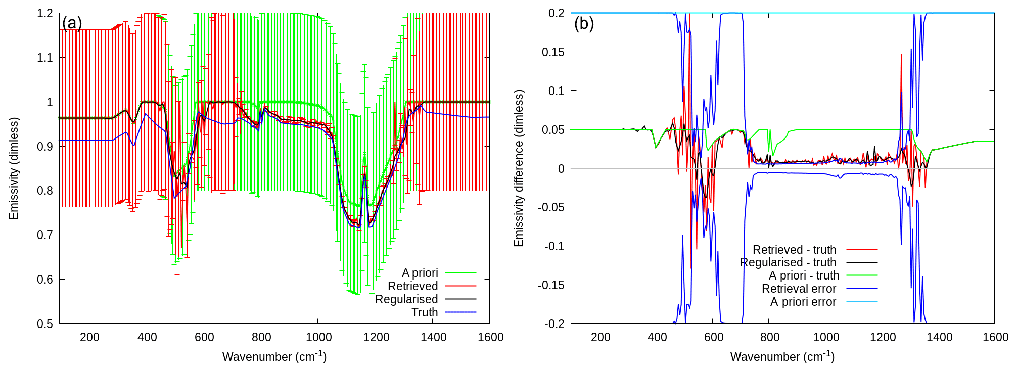
Figure 12Emissivity retrieval for case 1.1 (desert at noon in summer). The a priori error is set to 0.2, and a posteriori regularization is applied. (a) A priori profile with error bars (green), retrieved profile with error bars (red), regularized retrieved profile (black), and truth (blue). (b) Difference between retrieved and true (red) and retrieval error (blue), difference between regularized and model (black), and difference between a priori and model (green) and a priori error (cyan).
With sensitivity tests, we discovered that the bias does not depend on the particular choice of the spectrum noise. Also, the bias shows up also when retrieving only emissivity and skin temperature. The sign of the bias depends on the sign of the perturbation of the a priori emissivity, while the initial guess of the emissivity and the initial guess and a priori of the surface temperature have no effect. The effect is due to a strong anticorrelation between retrieved emissivity and surface temperature, which reaches −0.8 in the MIR region (see also the right panel of Fig. 13). There are different ways of solving this problem, and ad hoc studies to optimize the retrieval settings are under way. In particular, the use of a coarser emissivity grid has to be considered. One of the solutions is to use a larger a priori emissivity error, i.e., 0.2. A larger error of the a priori, however, produces oscillations in the retrieved emissivity due to the weaker constrain, which can be reduced by extending the IVS regularization to the emissivity. The results are shown in Fig. 12.
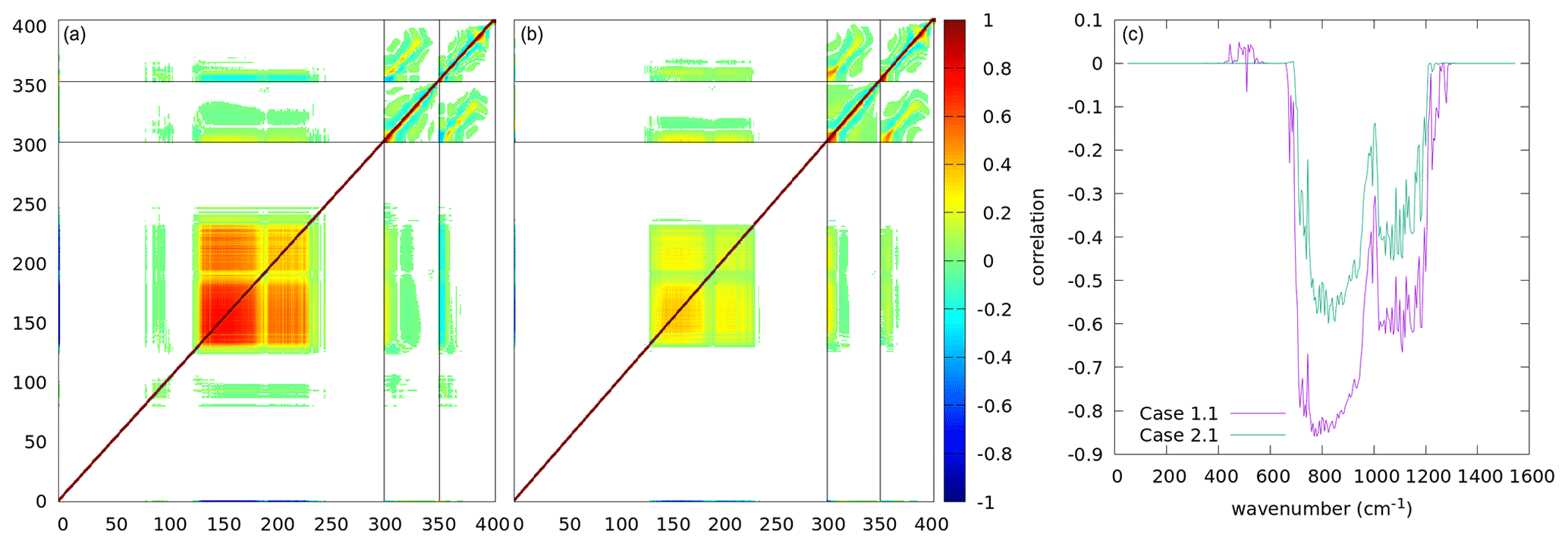
Figure 13Correlation matrices for cases 1.1 (a) and 2.1 (b). The x and y axes represent the retrieval vector element index. Lines are drawn to separate the surface temperature and emissivity sector (lower indices) from temperature (middle indices) and water vapor (higher indices). Points with a positive or negative correlation less than 0.01 are not drawn to enhance the readability of the figure. In panel (c), the correlation between the surface temperature and the emissivity is explicitly shown for the two cases.
In Fig. 13, we show the correlation matrices for the retrieved quantities in the case 1.1 (desert) and 2.1 (water). The right panel contains the correlation of the surface temperature with regard to the surface emissivity in the retrieval of both cases, i.e., the rows of the leftmost columns of the two other panels corresponding to emissivity. Again, we remark the strong anticorrelation between the two quantities in the retrieval, which reaches its maximum in the desert case.
5.2 Homogeneous cloudy-sky cases
The second group of tests still deals with the homogeneous case but for a cloudy sky. The retrieval module used for the E2ES project only retrieves cloud properties in cloudy conditions. The aim of these tests is to show that, even when using a perturbed atmosphere, we are still able to retrieve the cloud properties with a good precision.
The quantities retrieved in the cloudy-sky case are the top of the cloud, the equivalent radius of the particle, and the total optical depth of the cloud. We realized that there is no sensitivity to the geometrical thickness of the cloud, so we assumed this parameter to be constant. The tests were performed analyzing the simulated E2ES FORUM observations related to the first six homogeneous scenarios described in Table 4 for cloudy-sky conditions.
5.2.1 Comparison with SACR code
The SACR code is able to perform the simultaneous retrieval of the atmospheric state and ice cloud parameters, and it was applied to the analysis of the spectral measurements acquired by the REFIR-PAD spectroradiometer, which has been operational at the Concordia Station on the Antarctic Plateau since 2012 (Palchetti et al., 2016; Di Natale et al., 2017). The SACR code (Di Natale et al., 2020) performs the retrieval of water vapor and temperature profiles, the surface temperature, the cloud position, and the cloud optical and microphysical properties, such as the generalized ice and water effective diameter, the ice fraction, and the optical depth or the ice water path (IWP). To simulate the atmospheric radiative transfer, the LBLRTM is integrated with a specifically developed subroutine based on the Delta–Eddington two-stream approximation, whereas the single scattering properties of cirrus clouds are derived from a database for hexagonal column habits. To perform the retrieval procedure, SACR code uses the optimal estimation method with the Levenberg–Marquardt approach.
The L2 products obtained from the L2M_I and SACR are compared here. To perform a realistic validation, the atmospheric state used in the retrieval procedure is perturbed with respect to the true state, according to the CM of the a priori. In the E2ES project, the atmospheric parameters are not retrieved. Due mainly to the differences in the cloud representation, we cannot truly speak of validation in the cloudy case. In order to obtain similar results, the initial guess, a priori, and a priori errors for the SACR code were taken from the output of the L2M_I preprocessor and not from the CIC estimate. The aim of the comparison is to show that the retrieval module of the E2ES and the comparative code have similar capabilities at identifying cloud properties, thus confirming that the results are not code dependent.
5.2.2 Discussion of the results
The results for the five cloudy cases (the coastal marine case was wrongly attributed by the CIC to a clear-sky retrieval due to the small contrast between the cloud and the surface, and case 7 was only studied in clear-sky conditions) are summarized in Table 10.

We see that, qualitatively, the results obtained by the two codes are similar. With some exceptions, the retrieved cloud parameters are very close to the true parameters – even if the retrieved parameters are characterized by very small errors – in most cases, the difference between the retrieved and the true value is larger than the error.
In the E2ES, the cloud composition and scattering properties are the same in the simulation and retrieval of data, so the model error, which is significant with real data and must be accounted for in the CM, does not impact on the retrieval error.
On the other hand, there is the following combination of factors that explains the small error bars:
-
The error on the assumed atmosphere, which is perturbed with respect to the true state, is not taken into account in the error budget.
-
The linear estimate may not be verified, especially when parameters with different behaviors are mixed.
-
In presence of non-negligible correlations in the covariance matrix, differences between the retrieved value and the true state can be larger than the square root of the diagonal matrix. The typical absolute values of the cloud parameter correlations are in the 0.1–0.7 range.
The retrieval of cloud parameters may be critical even when cloud composition and scattering properties are perfectly known. The following examples list the critical aspects of the retrieval:
-
A water cloud at very low altitudes (case 3.2) that is not identified because the cloud and surface effects are similar.
-
A cirrus cloud which combines scattered radiation from below the cloud and direct radiation from above the cloud in the TOA spectrum. This combination leads to the existence of local minima in the cost function, which is minimized by the retrieval procedure, because different parts of the spectrum are well fitted by different cloud parameters. If the initial guess is far from the true values, then the retrieval may converge to a local minimum. This problem is tackled by the L2M_I by using a cloud preprocessor, as already mentioned. If the preprocessor is not used, then the results of both the L2M_I and SACR for cases 1.2 and 2.2 worsen.
-
A cloud characterized by a very large OD (case 6.2), where the sensitivity to the OD is lost. In this case, the cloud becomes fully opaque, and the only radiation seen by the instrument comes from above the cloud. The error on the spectrum, using an OD =10 instead of the true value OD =300, is smaller than the requirement for the NESR and can be seen in Fig. 14.
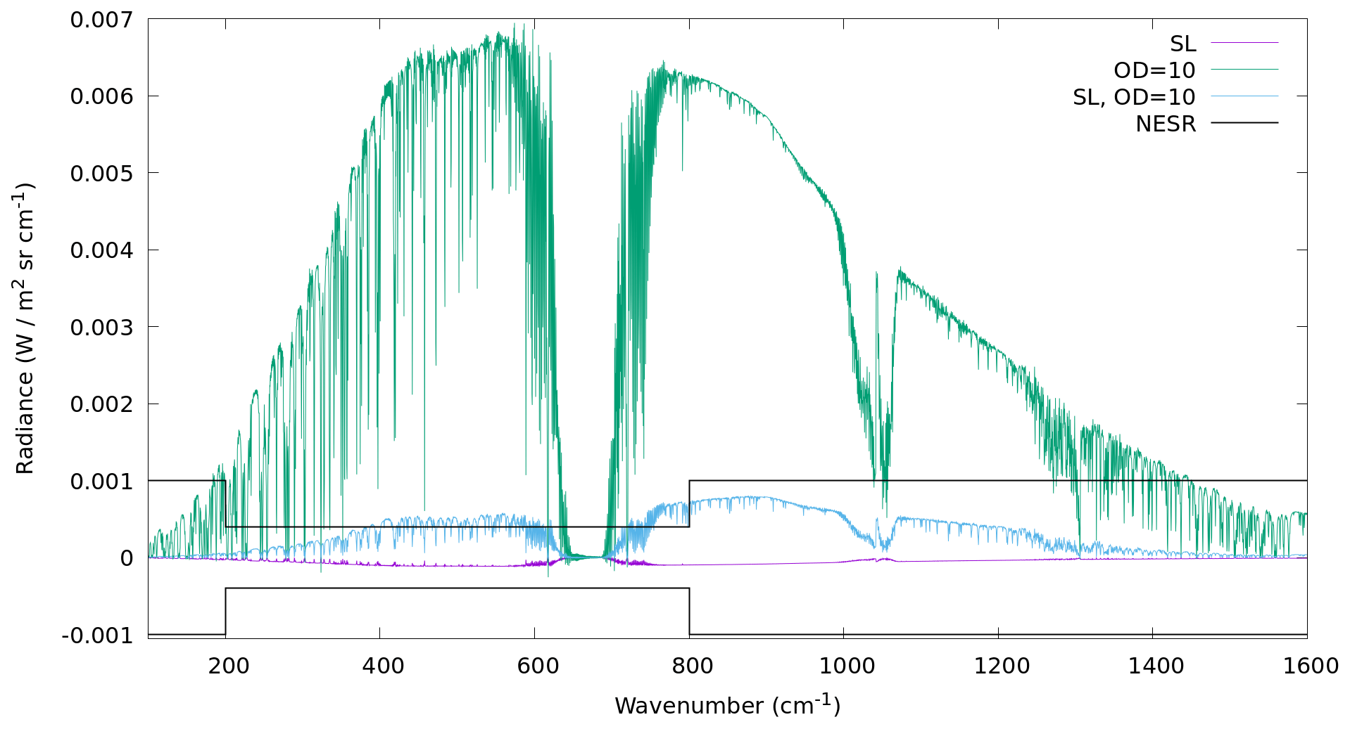
Figure 14Very thick cloud case (case 6.2; OD =300). A quantification of the error in the radiance is compared with the noise requirements (black curve) using the single layer (SL) approximation (purple curve), maximal OD of 10 (green curve), or both (blue curve).
For thick clouds, two L2M_I approximations were tested in order to reduce the computation time. A maximum OD was set to 10, and we represented the cloud as a single layer (SL) instead of multiple layers. The results are presented in Fig. 14.
The OD limit of 10, if used alone, introduces an error which is larger than the NESR because some radiation manages to penetrate the first layers of the cloud. The error is comparable with the NESR if the SL approximation is also applied because the compactness of the cloud impedes the penetration of the radiation. Indeed, the error becomes negligible if only the SL approximation is used, and the speedup is stunning. The fDISORT computation time with the SL approximation is about one-tenth of the computation time when no approximation is applied. On the other hand, the OD limit only subtracts some seconds. Thus, the retrievals were performed using the SL approximation. The drawback is that the sensitivity to large values of the OD is even smaller since the cloud is more compact.
5.2.3 Sensitivity to thin cirrus clouds
The far-infrared part of the spectrum is particularly sensitive to cirrus clouds, and recently, simulations were used to show that FIR can contribute to improving the detection of thin cirrus clouds (Maestri et al., 2019b, a; Magurno et al., 2020). The analysis with the E2ES allows us to evaluate the capability of retrieving cloud information from these measurements, also in presence of very thin cirrus clouds, and to compare the lowest detectable optical depth for a cirrus cloud by FORUM (range 100–1300 cm−1) with the one obtainable from the analysis of MIR measurements only (range 667–1300 cm−1). The sensitivity of the retrieval to the optical depth of the cirrus cloud depends on the contrast between the surface and the cloud, and this depends on the characteristics of the surface and the atmosphere. There were two cases considered for this analysis, namely cirrus on the desert and cirrus on the sea (see Table 5). The surface properties are assumed to be homogeneous for the entire scene.
For both cases, we started from the optical depth value of the considered case, and then we progressively halved the optical depth while keeping all other parameters unchanged until the CIC tool continued to classify this case as cloudy. Then L2M_I retrieval was performed to be sure that the retrieval was able to retrieve the cloud parameters. Contrary to previous tests where perturbed values of the truth were used for water vapor, temperature, and surface temperature, for these tests they were set to the true values to avoid a situation where a different error in temperature and water vapor had a different impact in the retrievals performed in the two different spectral regions. The results for the two considered cases are reported in Table 11.
Table 11Cirrus cloud cases 1.2 (cirrus on desert) and 2.2 (cirrus on ocean). Either the minimum optical depth that can be detected when either all FORUM spectrum is used (FIR+MIR) or only the MIR part (667–1100 cm−1) is used.
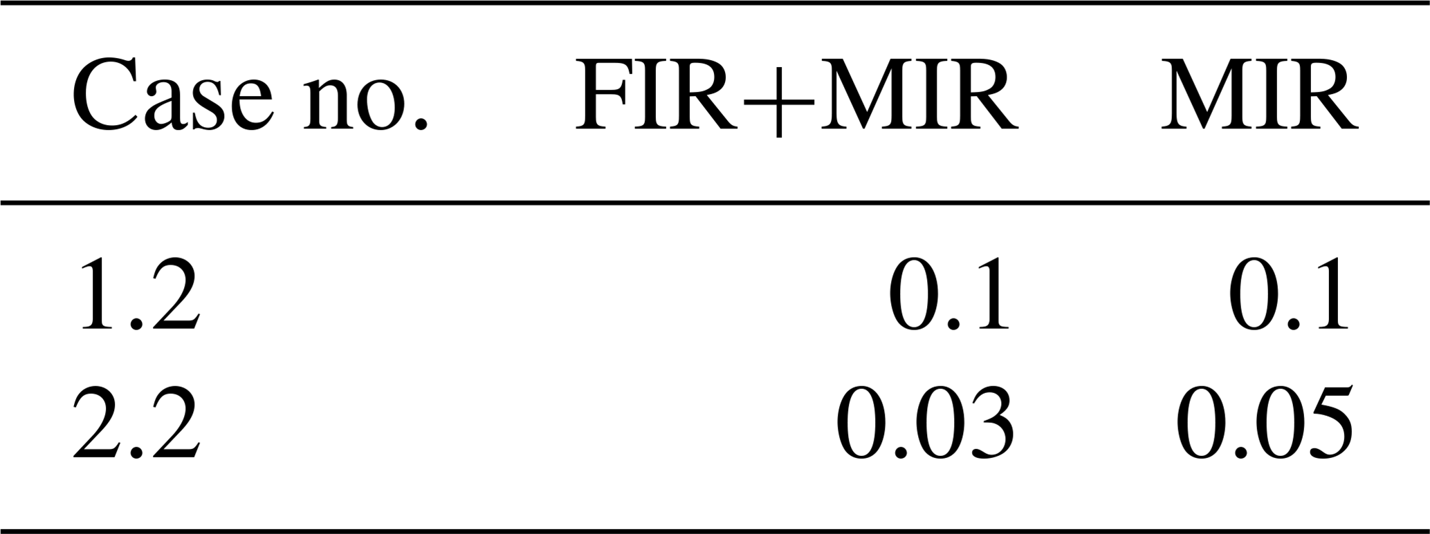
For case 1.2, the minimal optical depth was 0.1 for both MIR and FIR+MIR, while for case 2.2, the minimal optical depth was 0.05 when only MIR measurements are used and 0.03 when both FIR and MIR bands are combined. The addition of the FIR band reduces the retrieval error and enhances the accuracy of the retrieval.
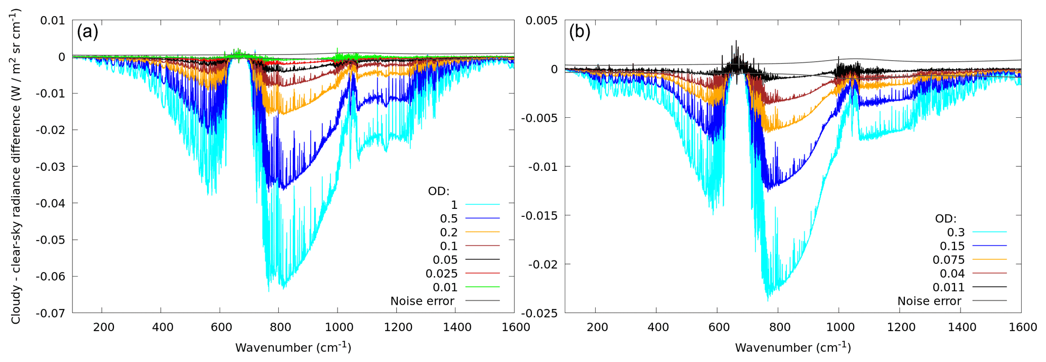
Figure 15Difference between the TOA radiance in the cloudy case for various optical depths of the clouds and the clear-sky case of case 1.2 (a) and case 2.2 (b), compared with the measurement error.
Figure 15 reports on the differences between the cloudy spectra relative to various optical depths and the clear-sky spectrum in both cases, compared with the random measurement error. Clouds are detectable and cloud parameters retrievable until the contribution of the cloud to the spectrum is larger than the noise. In real life, where the knowledge of the atmospheric profiles is affected by an error and in presence of other systematic errors, the retrieval of the cloudy quantities may be more difficult, but the information provided by this test represents the goal we can aim to reach.
5.3 Tests on heterogeneous cases
Given the extension of the FSI pixel, the probability that the scene might be heterogeneous is very high. The heterogeneity of the pixel poses different problems in the retrieval of L2 products (either atmospheric profiles, surface temperature and emissivity, or cloud information) from TOA radiance. The first issue is that the ISRF is modeled assuming a homogeneous FoV. If the FSI FoV is strongly heterogeneous, the ISRF may not represent the instrumental response well, thus introducing an error in the retrieval. In the case in which some predominant homogeneous characteristics can be identified in the heterogeneous scene, it is useful to quantify the error in the retrieval of the predominant homogeneous contribution due to the contamination of the scene with clouds or heterogeneities in the surface. On the contrary, if the scene is so heterogeneous that predominant homogeneous characteristics cannot be identified, then the measured spectrum has a value in itself, but the information extracted by the L2 analysis is just a combination of contributions coming from the different parts of the sounded atmosphere and surface. The different types of heterogeneities that can occur in the pixel are manifold, and the impact of heterogeneities in different scenarios can be very different. A large effort in the SGM was devoted to the handling of heterogeneous scenes, primarily to study the impact of these heterogeneities on the spectrum and then on the retrieved quantities. In the standard approach used by the L2M module, the pixel is assumed to be homogeneous, and the retrieval is performed in either clear-sky or cloudy-sky conditions on the basis of the CIC estimates. Thus, at the moment, we regard any heterogeneity of the FSI FoV as being a contamination of either a clear or a cloudy homogeneous scene.
5.3.1 Heterogeneities in the FSI FoV: convolution with ISRF
The objective of this test is to check whether the ISRF, which is modeled assuming a homogeneous FSI FoV, also allows a good representation of the FSI spectrum in the presence of heterogeneities in the FSI FoV. The OSS is able to accurately reconstruct the radiance seen by the instrument, thus taking care of the different beams coming from different parts of the FoV. The L2M simulates the spectrum observed by the instrument by convolving the high-resolution spectrum generated by the forward model with the ISRF computed assuming a homogeneous FoV, and hence, the deformations in the ISRF introduced by the heterogeneities are neglected. This may have a large impact on the quality of the retrieval, since the information on the profiles at the different altitudes comes from the knowledge of the line shapes of the spectral lines. The magnitude of the impact depends on the heterogeneities which are considered. Given the cylindrical symmetry of the FSI, heterogeneities in the FoV that are expected to mostly affect the ISRF are the ones that have a strong dependence on the radius.
To this end, we performed the following test. In the homogeneous case 1.1, we considered the spectrum calculated by the OSS and the one obtained by convolving the high-resolution spectrum generated by SGM with the ISRF. We compared the difference between these two spectra with the error noise. We then repeated the same comparison, using a cirrus cloud covering only part of the pixel in the center of the FoV this time.
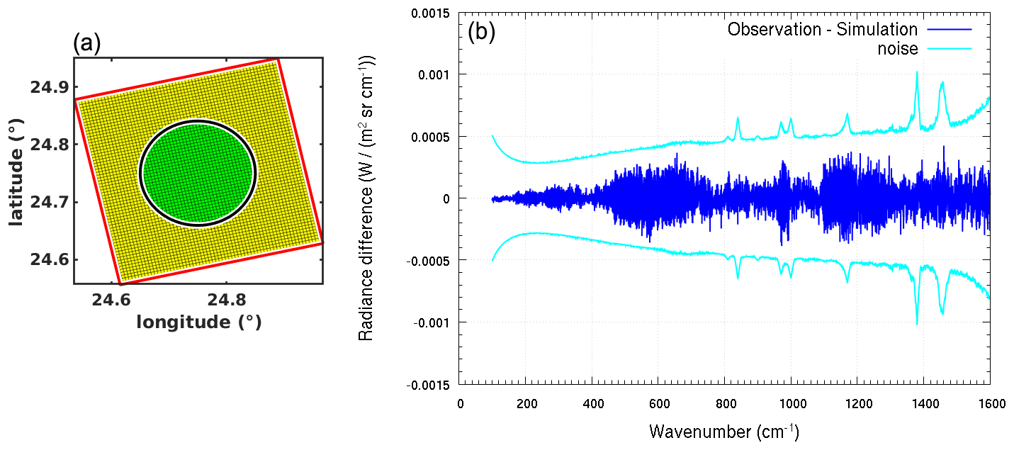
Figure 16(a) FORUM FoV, with FEI FoV (yellow) and FSI FoV clear (green). (b) Difference between the output radiance of the FSI and the high-resolution SGM radiance convolved by L2M with the ISRF, compared with measurement noise, in the homogeneous case.
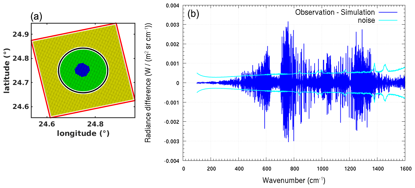
Figure 17(a) FORUM FoV, with FEI FoV (yellow) and FSI FoV clear (green) and cloudy (blue). (b) Difference between the output radiance of the FSI and the high-resolution SGM radiance convolved by L2M with the ISRF, compared with measurement noise, in the heterogeneous case.
Figures 16 and 17 show, respectively for the homogeneous case and the heterogeneous one, the FSI FoV and the difference between the output radiance of the FSI, as calculated by the OSS, with the radiance obtained by convolving the high-resolution spectrum computed by SGM with the ISRF. This difference is plotted as a function of the wavenumber together with the measurement noise.
In the case of a homogeneous scene, the convolution with the ISRF is a good representation of the instrumental response. On the contrary, when strong heterogeneities are present, the convolution with the ISRF introduces an error larger than the measurement noise. In principle, the error coming from the representation of the ISRF cannot be neglected in the presence of large discontinuities such as the ones we have considered. In any case, the heterogeneity of the scene poses problems to the retrieval module, which considers the scene to be homogeneous. Also, the meaning of the retrieved quantities is uncertain, since the measured spectrum represents a kind of average of the different scene characteristics.
In the future, the L2M approach can be developed to use information coming from the FEI image and chi-square to identify and define dedicated strategies for heterogeneous scenes.
5.3.2 Cloud contamination of clear-sky FoV
This test aims at estimating the impact that an unidentified cloud contamination of the FSI FoV has on the retrieval, when performed with the assumption of clear-sky conditions, of temperature and water vapor profiles and of the surface temperature and frequency-dependent emissivity. The test is performed by simulating a clear-sky scene with the SGM, which is progressively contaminated by a cloud entering in the FSI FoV. This is the most simple and idealized case, with only two distinct FoV fractions that are internally homogeneous being investigated as a reference case. In real conditions, larger heterogeneities can be observed within the FoV. For this specific test, the study cases 1.1 and 1.2 (tropical profile on desert surface) are used, with the contaminating cirrus cloud as in test 1.2. The surface properties, and the atmosphere, are assumed to be homogeneous for the entire scene. The FoV fraction occupied by the cloudy sector is increased at steps of 2.5 %, from 0 % to 10 %, and then at steps of about 7 % up to cloud coverage fractions of 25 %.
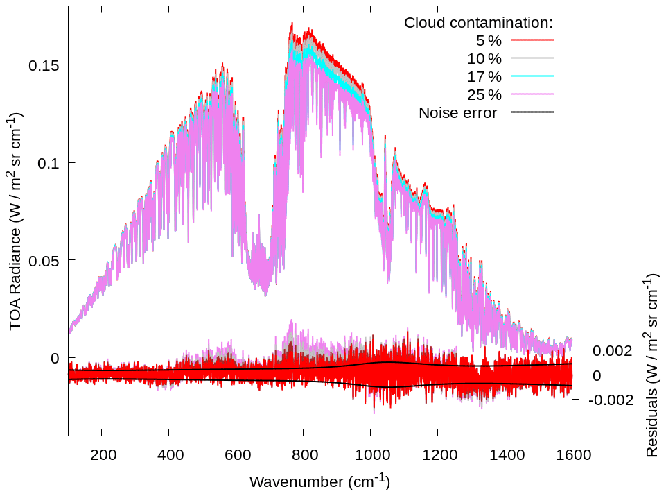
Figure 18 reports on the simulated spectra and residuals of the fit in the various cases. We note that, by increasing the cloud contamination, the residuals depart from purely random ones since the retrieval is not able to compensate for the cloud contamination by changing the retrieved quantities.
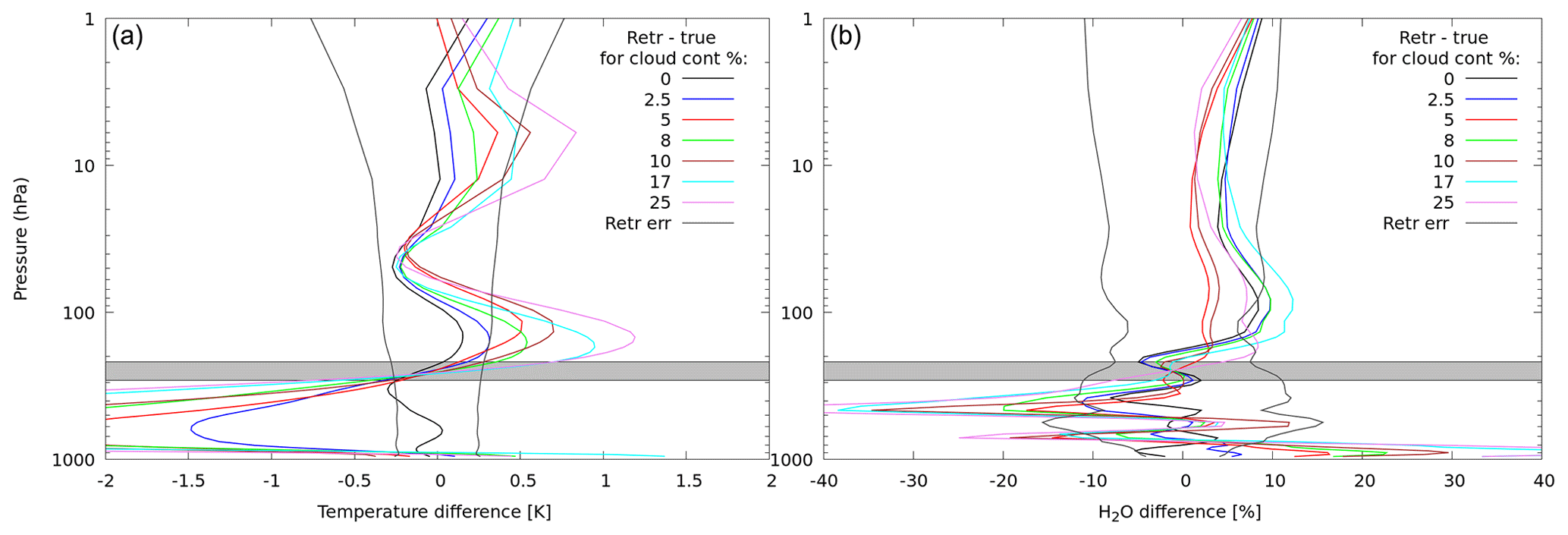
Figure 19Difference between retrieved and true profiles for temperature (a) and water vapor (b) for different percentages of cloud contamination in the FSI FoV, compared with the retrieval noise. The cloud pressure range is reported in gray.
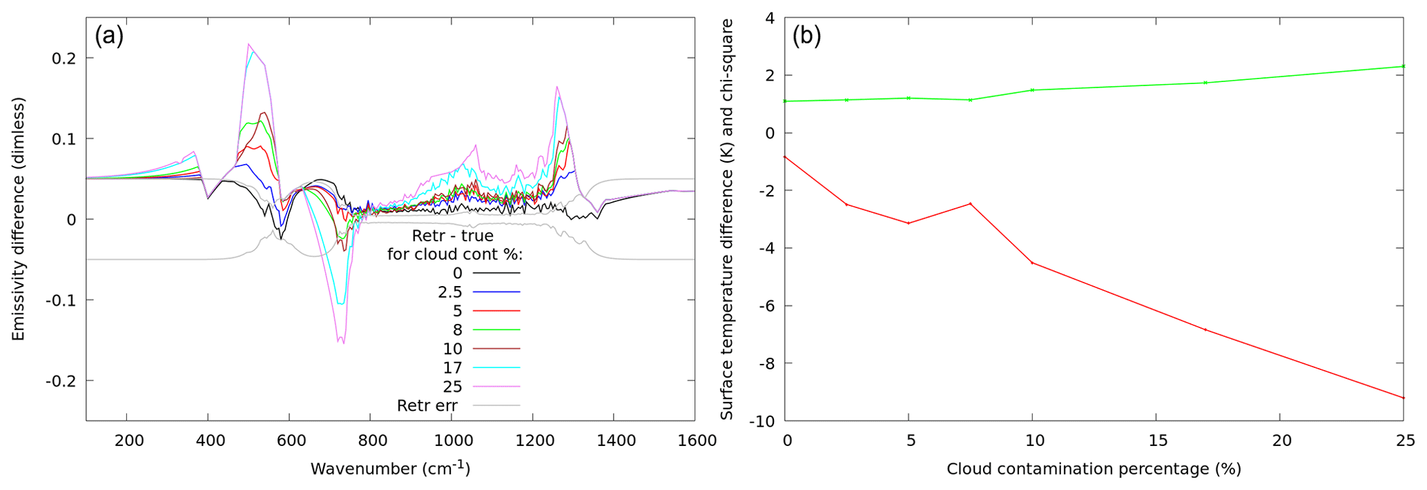
Figure 20(a) Difference between retrieved and true values of surface emissivity for various percentage of cloud contamination in the FSI FoV, compared with the retrieval noise. (b) Difference between retrieved and true values of surface temperature for various percentages of cloud contamination in the FSI FoV, compared with the retrieval noise. The final chi-square values are also reported.
The retrieval is performed for each simulation by assuming clear-sky conditions, and the retrieved quantities are compared with the values used by the SGM to simulate the part of the scene in clear-sky conditions. These are indicated as the true values. Figure 19 shows the difference between the retrieved and true values for the temperature profiles (Fig. 19a) and the water vapor profiles (Fig. 19b) compared with the corresponding retrieval error for different cloud contamination percentages. In general, increasing the cloud contamination increases the difference of the retrieved temperature profile with respect to the true expected values. In the worst case, at about 700 hPa, the differences increase from within the error for the completely clear-sky case (red line) up to about 6 times larger than the error for the clear case of 97.5 % and the cloudy case of 2.5 % (black line). Similar results, but with a reduced magnitude, are observed for the water vapor profile retrieval. The surface skin temperature retrieval is also affected by the cloud contamination. Figure 20 shows the difference between the true and the retrieved values of the surface emissivity as a function of the clear-sky FoV fraction (red line) and the corresponding χ2 values (green line). The differences in the retrieved temperature increase rapidly up to 3 K for a 5 % cloud contamination in the tested scenario. As described in Sect. 5.1.2, a negative bias in the surface temperature is compensated by a positive bias in the surface emissivity. Since the considered cloud is an optically thin cirrus cloud (OD =1), we expect that, for thicker clouds, such as in case of cumuli or cumulonimbus, the effects on the observed radiance and, hence, on the retrieved skin temperature are larger even for lower fractional areas. For the tested scenario, the quality of the retrieval is compliant with the E2ES requirements for a cloud contamination smaller than 10 %. Nevertheless, the CIC algorithm applied to the simulations identified the scene as cloudy as soon as the cloud fraction grew above 8 %. This means that the automatic inversion procedure would switch to the cloudy case and would not try to retrieve the surface properties in the worst scenarios, where the errors are too large, thus preserving the performance of the L2M_I.
5.3.3 Clear-sky heterogeneities in the surface
This test aims at evaluating the impact of the heterogeneity of the surface on the retrieval of the temperature and water vapor profiles. It is performed for a polar scene, since the largest amount of information on the surface is mainly obtained in the polar regions where the atmosphere is drier and, hence, more transparent. The scene at the geolocation corresponding to case 5.1 (polar case) is simulated, assuming that the surface has a part covered with fine snow and a part covered with sea. The surface temperature used to generate observations changes accordingly, with 273.27 K on water and 254.45 K on snow. Temperature and water vapor profiles are assumed to be homogeneous in the sounded atmosphere over the pixel. We used 1 for emissivity a priori and 253.423 K for surface temperature, which is a perturbation of the snow value. Results are shown for the scenes covered with different percentages of water and snow.
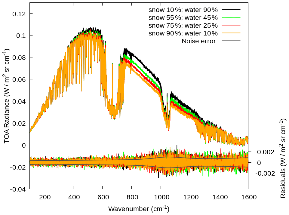
Figure 21Simulated radiances and residuals of the fit for different percentages of water or snow FoV coverage are indicated in the legend.
Figure 21 reports on the simulated spectra and residuals of the fit for different percentages of water/snow FoV coverage (snow at 10 %, 55 %, 75 %, and 90 %). The residuals in all cases are compatible with the measurement noise and show no bias.
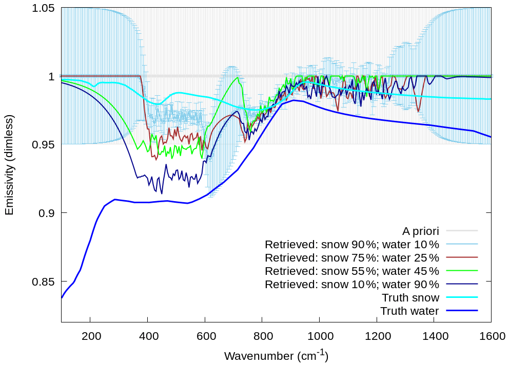
Figure 22Surface emissivity retrieved profiles for different types of soil heterogeneity and true profiles for homogeneous snow (cyan) and water (blue) soils. The used a priori profile and relative error are shown in gray. For readability reasons, the retrieval error is shown only for one case (snow 90 %–water 10 %), but the other cases are characterized by similar errors.
Figure 22 reports on the retrieved emissivity in the various cases, while the retrieved surface temperature is reported in Table 12.
Table 12Retrieved surface temperature for different percentages of water or snow FoV coverage.
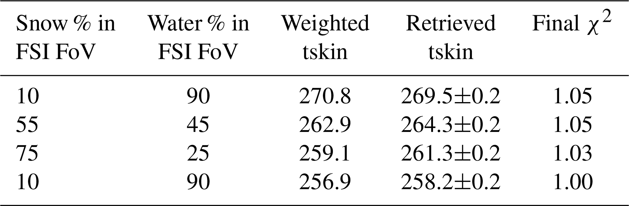
In all cases we find that retrieval of surface emissivity, and surface temperature, adapts in an almost linear way to handle the different percentage of snow or water pixel coverage; particularly in the spectral region between 400 and 600 cm−1, where water and snow emissivity mostly differ, the retrieved emissivity is closer to the water or the snow surface emissivity, according to the predominance percentage of the surface type in the pixel coverage. Differences between retrieved products and the weighted mean of the emissivities characterizing the different pixels of the FoV have to be attributed to the negative correlation between surface temperature and emissivity. On the contrary, the retrieved water and temperature profiles are little affected by the surface heterogeneities, since the differences between the retrieved value and the true one are always within the retrieval error (see Fig. 23).
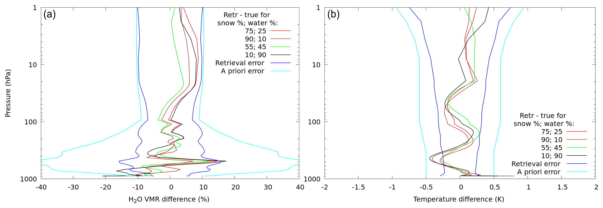
Figure 23Differences between retrieved and true profiles for different types of soil heterogeneity for temperature (a) and water vapor (b). Retrieval and a priori errors are also shown.
5.3.4 Tests based on MODIS L2 products
All of the previously investigated scenarios rely on idealized conditions, where the surface and, eventually, the cloud layer can only have homogeneous properties within the FSI FoV or a simple binomial characterization. This simplified scene description is convenient for evaluating study case scenarios and guaranteeing a good computational speed of the E2ES chain. Unfortunately, the real world is far from being ideal, and almost homogeneous conditions are more likely the exception rather than the rule. Surface, atmosphere, and cloud properties can significantly vary on spatial scales of the order of few kilometers or fewer, and their effects combine into a single 15 km diameter FoV FSI observation.
This last test aims at evaluating the E2ES performance in case a realistic, largely heterogeneous scene is ingested by the L2M module. In total, three complex case studies are generated with the SGM, i.e., a clear-sky case (M.1) over land, where the scene heterogeneity depends on the surface properties (temperature and emissivity) and on the atmospheric profiles (temperature and water vapor concentration), and two cloudy-sky scenes over land (M.2) and sea (M.3), where the clouds' inhomogeneities sum up with those of surface and atmosphere. Close locations in southern England are selected, and their geolocations and times are reported in Table 13.
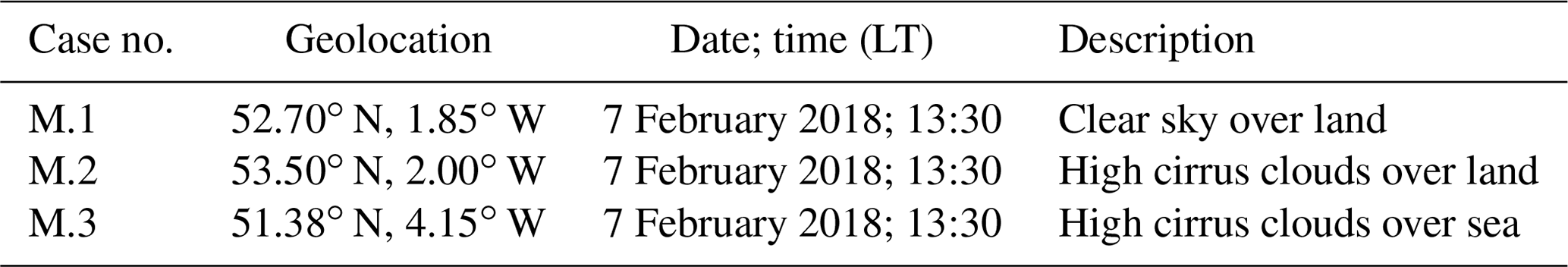
The surface, atmospheric, and cloud parameters used to build the scene are derived from the following databases:
-
The surface emissivity information is derived from the Global Land Cover Map (GlobCover 2009; http://due.esrin.esa.int/page_globcover.php; last access: 22 January 2022) is an ESA composite product based on MERIS (Medium Resolution Imaging Spectrometer Instrument) data collected at 300 m spatial resolution. The GlobCover map provides 22 land cover classes, defined with the United Nations land cover classification system, that are associated to the 11 surface types from Huang et al. (2016) used in the SGM surface definition.
-
The information on atmosphere is derived from the MODIS Atmospheric Profile product (07_L2; https://modis-images.gsfc.nasa.gov/products.html; last access: 22 January 2022), which defines the temperature and water vapor profiles and the surface height at 5 km resolution.
-
The cloud properties and surface temperature information from the MODIS Cloud Product (06_L2) are used to define the cloud parameters (particles phase and effective radius, cloud-top height, and optical thickness) and the surface temperature, with a spatial resolution of 1 km.
The above products are characterized by different grids and spatial resolutions; thus, they are remapped into the FEI grid. Once the cloud, atmospheric, and surface information are available at the same grid, a dedicated subroutine, mimicking the SGM, is applied to compute the spectral radiance for each pixel. Due to the complexity of the process, the subroutine is kept external to the E2ES chain. Nevertheless, following the above procedure, multiple scenarios can be built from satellite products for complex atmospheric conditions. The radiances are stored in the E2ES as ancillary data and are used for testing the FORUM E2ES performances on realistic conditions.
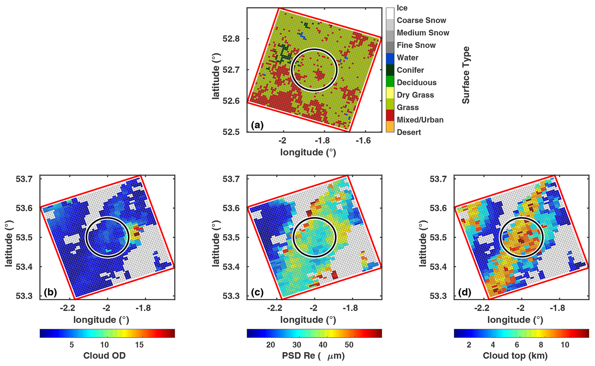
Figure 24(a) Surface type for the study case M.1, derived from GlobCover database and remapped on the FEI grid. The FSI FoV is marked with the black ring. Also shown are the cloud optical depth at 900 cm−1 (b), PSD effective radius (c), and cloud-top height (d) for the study case M.2, as derived from MODIS L2 data and remapped on the FEI grid. White areas indicate clear sky.
Figure 24 shows examples of the surface and cloud parameters remapped into the FEI grids. The scene observed in the M.1 clear-sky case (Fig. 24a) has irregularly sparse urban areas (brown) surrounded by different kinds of vegetation (light and dark green) and few wet areas (blue; probably lakes or ponds), creating a much more complex scenario than an ideal homogeneous case. Similarly, clear-sky areas alternate high- and low-level clouds, with unevenly distributed optical and microphysical parameters, in the M.2 cloudy case (Fig. 24b–d). Multiple spectral radiances are computed by the SGM for all the FEI grid points within the FSI FoV (the black circle in the panels of Fig. 24), according to the different properties of the scene. Within the E2ES, the precomputed radiances are ingested by the FSI-OSS module to produce a single spectral radiance. In Fig. 25, the spectral radiances computed for each FEI pixel inside of the FSI FoV (by using the dedicated subroutine mimicking the SGM) are plotted together with the FSI-OSS output radiance for the cases M.1 and M.2. The figure also reports on the radiance measurements in multiple MODIS channels (red dots) together with their variability within the FSI FoV. Note that the FSI-OSS spectral radiance based on MODIS products and the mean MODIS radiance at specific bands are consistent, but a perfect match is not expected due to the nonlinearity between L2 products and the radiance.
Finally, the L2M is used to retrieve the characterizing parameters of the complex scenes, in particular: temperature and water vapor profiles, and surface skin temperature and emissivity for the case M.1, correctly classified by CIC as a clear-sky scene; cloud properties for the cases M.2 and M.3, classified by CIC as a cloudy scene.

Figure 25Spectral radiances computed by using the dedicated subroutine mimicking the SGM (gray lines) for each FEI pixel within the FSI field of view are plotted with radiances obtained from the FSI-OSS (black lines) for the cases M.1 (a) and M.2 (b). The MODIS radiance at specific bands is also indicated with red dots. The vertical red bars indicate the MODIS radiance variability within FSI FoV.
In the analyzed realistic cases, it is not possible to define a single “truth” to be compared with the retrieval results. The average parameters within the FSI FoV do not properly describe the scene as a whole. To evaluate the L2M_I performance, the assessment test verifies that the retrieved scalar quantities lie within 1 standard deviation from the average value and that spectral quantities and profiles are consistent, within the error bars, with the bulk of the input values.
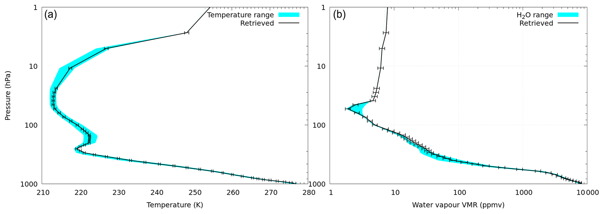
Figure 26Comparison between the retrieved profiles and the reference profiles for the clear-sky case M.1. (a) Temperature profile range in the FoV and retrieved profiles, with the retrieval error and the water vapor profiles range for the FoV and retrieved profile with retrieval error shown. (b) Emissivity profiles, with percentages in the FoV pixels, a priori, weighted-emissivity average, and retrieved profile with retrieval error, are shown.
Figure 26 shows the retrieval results (black curves) of the clear-sky case M.1. The retrieved temperature and water vapor profiles are compared with the range of the reference profiles that are considered for the SGM simulation within the FSI FoV, as derived from the MODIS L2 data. The retrieved profiles are consistent with the input profiles along the entire vertical extension of the model.

Figure 27Emissivity profiles, with percentages in the FoV pixels, a priori, weighted-emissivity average, and retrieved profiles with retrieval error, are shown.
In Fig. 27, the emissivity retrieval is reported. As already shown in Sect. 5.1.2, the sensitivity to surface emissivity at middle latitudes is limited to the spectral range of 700–1300 cm−1 because of the large absorption of water vapor in the FIR. We show the emissivity profiles used by the SGM along with the percentage of the FoV pixels. The retrieved emissivity in the atmospheric window is very close to the weighted average of the input profiles, suggesting the capabilities of the inversion procedure in a complex scenario. Finally, the model surface skin temperature of 275.96±0.05 K is well reconstructed by the retrieved value 276.12±0.39.
Table 14Cloud parameter results for cloudy MODIS cases M.2 and M.3.

Table 14 shows the retrieval results for the two cloudy-sky cases of M.2 and M.3, respectively. The retrieved cloud parameters (optical depth, PSD effective radius, and cloud-top height) are scalar values; therefore, they are compared with the range of the same parameters for all the FSI FoV subpixels. As in the previous case, despite the heterogeneity of the observed scene, the L2M retrieves values that are in the range of the observed scene. There is a slight tendency to overestimate the particle radius, but for large particles, there is no sensitivity in the measurements. These tests further confirm the good performance of the E2ES as a tool for the analysis of ideal and realistic study cases.
The E2ES was not designed with computing time optimization in mind. For this task, an adaptation to FORUM of fast-forward models, such as σ-IASI (Amato et al., 2002), would be more adequate. However, in order to run all of the tests, some effort has been devoted to speeding up the code. Almost all the computing time of the E2ES is spent on two tasks, and the remaining components affect the results only marginally.
-
The forward-model calculation, i.e., running LBLRTM in clear-sky cases and fDISORT in cloudy-sky cases. This task is performed by the SGM as many times as the number of non-homogeneous pixels in the scene and by L2M_I as needed by the retrieval sequence.
-
The ISRF convolution. This task is only performed by L2M_I. Given the frequency-dependent characteristic of the ISRF, the task needs to be performed in the radiance domain, and the FFT cannot be applied.
Of course the computing time heavily depends on the machine used and on the compiler. The figures presented refer to an Intel® Xeon® CPU E5-1650 v2 machine at 3.50 GHz with six physical cores, and to the Intel® Fortran (IFORT) compiler.
The scene preparation, consisting of reading the user input parameters and setting the input files for the forward computations, is very fast and typically lasts about 5 s.
The typical running speed for the LBLRTM, with an optimized spectroscopic database, is 35–40 s, with no major differences between scenes. The running time of fDISORT is the bottleneck of the cloudy retrieval, and it is heavily dependent on the cloud composition. A larger number of layers of the cloud, larger particles, and larger OD tend to increase the computation time of the multiple scattering effect. The running time of the fDISORT, if executed serially, varies from 20 min (cirrus clouds of case 1.2) to 30 h (thick opaque clouds of case 6.2). The fDISORT is itself between 1.2 (for liquid clouds) and 3.7 (for cirrus clouds) times faster than the original DISORT (Sgheri and Castelli, 2018). Applying the optimizations of Sect. 5.2.2, the thick cloud fDISORT is 10 times faster.
As for the convolution, a single operation takes about 20 s, but the task needs to be repeated at each iteration for each point of the vertical profiles of temperature and water vapor, plus two more times for skin temperature and emissivity. For clear-sky cases in the standard settings, we need 106 convolutions at each iteration.
The running time of the SGM in a homogeneous situation is approximately equal to that of the LBLRTM for the clear-sky cases and that of the fast LBLDIS (fLBLDIS) for the cloudy-sky cases. It is evident that, in the case of the MODIS scenes, where each subpixel of the FSI FoV is treated separately, the SGM radiances had to be precomputed because the calculations last several days, even with parallelization of the tasks.
The L2M_CIC module only takes less than 1 min to perform the land mask, the cloud identification and classification, the characterization of the level of inhomogeneities in the FSI pixel, and the preparation of the initial-guess inputs for the cloud retrieval.
For the L2M_I module, we take advantage of the multicore feature of the machine. The fDISORT is computed in parallel over different wavenumber intervals running multiple copies of the external binary, with results close to the theoretical maximum speedup. The convolution is computed using the multithread support of the OpenMP (OpenMP Architecture Review Board, 2018) libraries. With these settings, the effective running time is still affordable to run tests, even in cloudy-sky situations.
For the clear-sky cases, the running time of each iteration of the L2M_I module is about 20–25 min. The full L2M_I clear retrieval, including ancillary tasks, such as the additional forward model after the regularization to calculate the chi-square of the regularized solution, takes about 90 min for case 1.1 that uses four iterations.
For the cloudy-sky cases, the running time of each iteration of the L2M_I module varies from 10–12 min (case 1.2) to 90–120 min (case 6.2). In the cloudy cases, the longest execution time of the forward model is compensated by the fact that we only retrieve the cloud parameters using a constant perturbed atmosphere. The preprocessor, which is only enabled for cirrus clouds, takes about 30 min. The full L2M_I cloudy retrieval takes about 120 min, for case 1.2 that uses five iterations, and 440 min, for case 6.2 (the longest) that uses three iterations but also needs three Marquardt microiterations.
The findings of the FORUM E2ES project are presented. In the E2ES, the geometry of the orbit, the atmosphere, and the FSI and FEI instruments are fully modeled with realistic configurations, and retrieval is performed by assuming either full clear-sky or cloudy-sky scenes.
We first successfully validate the performances of the E2ES chain with correlative codes, which is a necessary step to ensure that there are no flaws. Then we select some homogeneous test cases, both in clear and in cloudy sky, which are chosen to represent all different atmospheric conditions, soil characteristics, and cloud types. In all cases, the retrieved quantities satisfy FORUM requirements. In cloudy sky, we also show that the optical depth threshold for a cirrus cloud to be detected varies between 0.03 and 0.1, with generally better sensitivity if the FIR is included. The threshold depends on the different characteristics of the surface and the atmosphere.
The influence on the retrieval of inhomogeneities in the field of view is also investigated. The convolution of the high-resolution spectrum with the ISRF function (computed assuming a model homogeneous FoV) represents the instrumental effects for a homogeneous FoV well, with the error being below the NESR threshold. This is not the case when a strong inhomogeneity is considered.
Heterogeneous soil in the FoV does not impact the retrieval of atmospheric profiles, with the retrieved surface temperature and emissivity approaching the weighted averages of the surface properties.
Even a small contamination of a cloud in the FoV induces errors in the retrieved atmospheric and surface quantities. The error increases with the increase in the percentage of the FoV affected by the contamination and of the optical depth of the cloud. However, it is important to underline that, by exploiting the information content of the FIR channels, the CIC algorithm is highly sensitive to the presence of a cloud in the FSI FoV, even with a low percentage of cloud contamination. Thus, in most cases, the cloud identification is performed and the performances of the L2M_I are preserved. Note that CIC is the first algorithm which exploits the far-infrared spectral interval for cloud identification and classification from satellite observations, including the determination of cloud phase. In particular, it is demonstrated that the combined use of FIR and MIR spectral radiances enhances the cloud detection performances achievable by using the MIR part of the spectrum only.
Finally, we perform the retrieval on some realistic heterogeneous scenes, which, however, present a predominance of either clear sky or cloudy sky. We show that the retrieval converges to values that are included in the range of variability in the quantities used to model the radiances.
Some critical problems have been highlighted. In particular, we believe that the following main issues should be investigated, also in the light of the synergy with IASI-NG.
-
Emissivity retrieval. The retrieval method and grid should be optimized as is clear from the tests in this paper. Some work is being done (Ben-Yami et al., 2021) in clear-sky conditions. The preliminary tests in cloudy-sky conditions, with an evolution of the code that simultaneously retrieves the atmospheric and cloud parameters, show that this issue will be even more important given the reduced sensitivity to the atmospheric surface due to the cirrus clouds.
-
Atmospheric retrieval in presence of thick clouds. In this case, there is no sensitivity to atmospheric parameters below the cloud top. A clear-sky retrieval can be attempted with the cloud top representing the bottom limit for the radiative transfer, similar to Feng et al. (2021).
-
Heterogeneous FoV. In this case, we might employ the FEI results to determine a homogeneity map for the various parts of the FSI FoV. This can be seen as an a priori to attempt a composite (partly clear and partly cloudy) retrieval.
In the FORUM E2ES contract, the open distribution of the code is not mandatory. Each author retains the intellectual property rights, or their portions, and the industrial partners of the consortium do not allow the distribution of their modules. The inversion module can be obtained from the corresponding author of this paper upon request.
The datasets used for retrieval for the cases mentioned in the paper are available at https://doi.org/10.5281/zenodo.5869329 (Sgheri, 2022).
All authors contributed to the writing of this paper. CB wrote the L2M Python wrapper. MBY performed some tests. GB was responsible for the OSS module and wrote the FSI code. BCD was the FORUM Phase A study manager. UC coordinated the contact between CNR and Deimos. SDB was responsible for the E2ES validation and performed the tests in clear sky. GDN performed the validation tests in cloudy sky. TG was the E2ES project manager, contributed the Geometry Module, and wrote the FEI and PAM modules. DL was the E2ES FORUM ESA's technical responsible representative during the FORUM Phase A and Phase B1. TM was responsible for the SGM module. TM, WC, and DM wrote the SGM and L2M_CIC codes. HO is the FORUM mission scientist. PR was responsible for the assessment campaign and performed most of the tests in this paper. CS performed some tests. LS was responsible for the L2M module, wrote the L2M inversion code, and coordinated the writing of this paper.
The contact author has declared that neither they nor their co-authors have any competing interests.
Publisher's note: Copernicus Publications remains neutral with regard to jurisdictional claims in published maps and institutional affiliations.
We would like to thank all the FORUM research group, a large and active community. Only by working together the FORUM project grew from an instrument concept to an operative mission.
This paper was edited by Simone Lolli and reviewed by two anonymous referees.
Amato, U., Masiello, G., Serio, C., and Viggiano, M.: The σ-IASI code for the calculation of infrared atmospheric radiance and its derivatives, Environ. Modell. Softw., 17, 651–667, https://doi.org/10.1016/s1364-8152(02)00027-0, 2002. a, b
Ben-Yami, M., Oetjen, H., Brindley, H., Cossich, W., Lajas, D., Maestri, T., Magurno, D., Raspollini, P., Sgheri, L., and Warwick, L.: Emissivity Retrievals with FORUM's End-to-end Simulator: Challenges and Recommendations, Atmos. Meas. Tech. Discuss. [preprint], https://doi.org/10.5194/amt-2021-232, in review, 2021. a
Bianchini, G. and Palchetti, L.: Technical Note: REFIR-PAD level 1 data analysis and performance characterization, Atmos. Chem. Phys., 8, 3817–3826, https://doi.org/10.5194/acp-8-3817-2008, 2008. a
Bianchini, G., Carli, B., Cortesi, U., Del Bianco, S., Gai, M., and Palchetti, L.: Test of far-infrared atmospheric spectroscopy using wide-band balloon-borne measurements of the upwelling radiance, J. Quant. Spectrosc. Ra., 109, 1030–1042, https://doi.org/10.1016/j.jqsrt.2007.11.010, 2008. a
Bianchini, G., Palchetti, L., and Carli, B.: Vectorial combination of signals in Fourier transform spectroscopy, Infrared Phys. Techn., 52, 19–21, https://doi.org/10.1016/j.infrared.2008.09.004, 2009. a
Bianchini, G., Castagnoli, F., Di Natale, G., and Palchetti, L.: A Fourier transform spectroradiometer for ground-based remote sensing of the atmospheric downwelling long-wave radiance, Atmos. Meas. Tech., 12, 619–635, https://doi.org/10.5194/amt-12-619-2019, 2019. a
Bozzo, A., Maestri, T., Rizzi, R., and Tosi, E.: Parameterization of single scattering properties of mid-latitude cirrus clouds for fast radiative transfer models using particle mixtures, Geophys. Res. Lett., 35, L16809, https://doi.org/10.1029/2008gl034695, 2008. a
Brindley, H. E. and Harries, J. E.: The impact of far i.r. absorption on clear sky greenhouse forcing: sensitivity studies at high spectral resolution, J. Quant. Spectrosc. Ra., 60, 151–180, https://doi.org/10.1016/s0022-4073(97)00152-0, 1998. a
Carli, B., Bazzini, G., Castelli, E., Cecchi-Pestellini, C., Del Bianco, S., Dinelli, B., Gai, M., Magnani, L., Ridolfi, M., and Santurri, L.: MARC: A code for the retrieval of atmospheric parameters from millimeter-wave limb measurements, J. Quant. Spectrosc. Ra., 105, 476–491, https://doi.org/10.1016/j.jqsrt.2006.11.011, 2007. a
Chahine, M. T., Pagano, T. S., Aumann, H. H., Atlas, R., Barnet, C., Blaisdell, J., Chen, L., Divakarla, M., Fetzer, E. J., Goldberg, M., Gautier, C., Granger, S., Hannon, S., Irion, F. W., Kakar, R., Kalnay, E., Lambrigtsen, B. H., Lee, S.-Y., Marshall, J. L., Mcmillan, W. W., Mcmillin, L., Olsen, E. T., Revercomb, H., Rosenkranz, P., Smith, W. L., Staelin, D., Strow, L. L., Susskind, J., Tobin, D., Wolf, W., and Zhou, L.: AIRS, B. Am. Meteorol. Soc., 87, 911–926, https://doi.org/10.1175/bams-87-7-911, 2006. a
Chen, X., Huang, X., and Flanner, M. G.: Sensitivity of modeled far-IR radiation budgets in polar continents to treatments of snow surface and ice cloud radiative properties, Geophys. Res. Lett., 41, 6530–6537, https://doi.org/10.1002/2014gl061216, 2014. a
Clough, S., Shephard, M., Mlawer, E., Delamere, J., Iacono, M., Cady-Pereira, K., Boukabara, S., and Brown, P.: Atmospheric radiative transfer modeling: a summary of the AER codes, J. Quant. Spectrosc. Ra., 91, 233–244, https://doi.org/10.1016/j.jqsrt.2004.05.058, 2005. a
Clough, S. A. and Iacono, M. J.: Line-by-line calculation of atmospheric fluxes and cooling rates: 2. Application to carbon dioxide, ozone, methane, nitrous oxide and the halocarbons, J. Geophys. Res., 100, 16519, https://doi.org/10.1029/95jd01386, 1995. a
Clough, S. A., Iacono, M. J., and Moncet, J.-L.: Line-by-line calculations of atmospheric fluxes and cooling rates: Application to water vapor, J. Geophys. Res., 97, 15761–15785, https://doi.org/10.1029/92JD01419, 1992. a
Cortesi, U., Bianco, S. D., Gai, M., Laurenza, L., Ceccherini, S., Carli, B., Barbara, F., and Buchwitz, M.: Sensitivity analysis and application of KLIMA algorithm to GOSAT and OCO validation – KLIMA-IASI, Final Report of Project ESA-ESRIN/Contract n. 21612/08/I-OL, Tech. Rep. IFAC-TSRR, IFAC-CNR, 2014. a
Cossich, W., Maestri, T., Magurno, D., Martinazzo, M., Di Natale, G., Palchetti, L., Bianchini, G., and Del Guasta, M.: Ice and mixed-phase cloud statistics on the Antarctic Plateau, Atmos. Chem. Phys., 21, 13811–13833, https://doi.org/10.5194/acp-21-13811-2021, 2021. a
Di Natale, G., Palchetti, L., Bianchini, G., and Del Guasta, M.: Simultaneous retrieval of water vapour, temperature and cirrus clouds properties from measurements of far infrared spectral radiance over the Antarctic Plateau, Atmos. Meas. Tech., 10, 825–837, https://doi.org/10.5194/amt-10-825-2017, 2017. a
Di Natale, G., Bianchini, G., Del Guasta, M., Ridolfi, M., Maestri, T., Cossich, W., Magurno, D., and Palchetti, L.: Characterization of the Far Infrared Properties and Radiative Forcing of Antarctic Ice and Water Clouds Exploiting the Spectrometer-LiDAR Synergy, Remote Sensing, 12, 3574, https://doi.org/10.3390/rs12213574, 2020. a, b
Di Natale, G., Palchetti, L., Bianchini, G., and Ridolfi, M.: The two-stream δ-Eddington approximation to simulate the far infrared Earth spectrum for the simultaneous atmospheric and cloud retrieval, J. Quant. Spectrosc. Ra., 246, 106927, https://doi.org/10.1016/j.jqsrt.2020.106927, 2020. a
Dinelli, B. M., Castelli, E., Carli, B., Del Bianco, S., Gai, M., Santurri, L., Moyna, B. P., Oldfield, M., Siddans, R., Gerber, D., Reburn, W. J., Kerridge, B. J., and Keim, C.: Technical Note: Measurement of the tropical UTLS composition in presence of clouds using millimetre-wave heterodyne spectroscopy, Atmos. Chem. Phys., 9, 1191–1207, https://doi.org/10.5194/acp-9-1191-2009, 2009. a
Dinelli, B. M., Labonnote, L., and Bianco, S. D.: Consolidated recommendations for updating the MRD regarding Level 1 data, and definitions, Technical Note 8, FORUMreq project: FORUM – consolidation of requirements and reference scenarios, 2020. a
Eremenko, M., Sgheri, L., Ridolfi, M., Cuesta, J., Costantino, L., Sellitto, P., and Dufour, G.: Tropospheric ozone retrieval from thermal infrared nadir satellite measurements: Towards more adaptability of the constraint using a self-adapting regularization, J. Quant. Spectrosc. Ra., 238, 106577, https://doi.org/10.1016/j.jqsrt.2019.106577, 2019. a
ESA: Earth Explorer 9 Candidate Mission FORUM, Report for Mission Selection ESA-EOPSM-FORM-RP-3549, European Space Agency, Noordwijk, The Netherlands, https://esamultimedia.esa.int/docs/EarthObservation/EE9-FORUM-RfMS-ESA-v1.0-FINAL.pdf (last access: 21 January 2022), 2019. a, b, c
ESA: Far-infrared-Outgoing-Radiation Understanding and Monitoring (FORUM) – Mission Requirements Document, Tech. rep., ESA, Earth and Mission Science Division, 2020. a
Feldman, D. R., Collins, W. D., Pincus, R., Huang, X., and Chen, X.: Far-infrared surface emissivity and climate, P. Natl. Acad. Sci. USA, 111, 16297–16302, https://doi.org/10.1073/pnas.1413640111, 2014. a
Feng, J., Huang, Y., and Qu, Z.: A simulation-experiment-based assessment of retrievals of above-cloud temperature and water vapor using a hyperspectral infrared sounder, Atmos. Meas. Tech., 14, 5717–5734, https://doi.org/10.5194/amt-14-5717-2021, 2021. a
Han, Y., Revercomb, H., Cromp, M., Gu, D., Johnson, D., Mooney, D., Scott, D., Strow, L., Bingham, G., Borg, L., Chen, Y., DeSlover, D., Esplin, M., Hagan, D., Jin, X., Knuteson, R., Motteler, H., Predina, J., Suwinski, L., Taylor, J., Tobin, D., Tremblay, D., Wang, C., Wang, L., Wang, L., and Zavyalov, V.: Suomi NPP CrIS measurements, sensor data record algorithm, calibration and validation activities, and record data quality, J. Geophys. Res.-Atmos., 118, 12734–12748, https://doi.org/10.1002/2013jd020344, 2013. a
Hansen, J. E.: Multiple Scattering of Polarized Light in Planetary Atmospheres Part II. Sunlight Reflected by Terrestrial Water Clouds, J. Atmos. Sci., 28, 1400–1426, https://doi.org/10.1175/1520-0469(1971)028<1400:msopli>2.0.co;2, 1971. a
Harries, J., Carli, B., Rizzi, R., Serio, C., Mlynczak, M., Palchetti, L., Maestri, T., Brindley, H., and Masiello, G.: The Far-infrared Earth, Rev. Geophys., 46, RG4004, https://doi.org/10.1029/2007RG000233, 2008. a
Hersbach, H., Bell, B., Berrisford, P., Hirahara, S., Horányi, A., Muñoz-Sabater, J., Nicolas, J., Peubey, C., Radu, R., Schepers, D., Simmons, A., Soci, C., Abdalla, S., Abellan, X., Balsamo, G., Bechtold, P., Biavati, G., Bidlot, J., Bonavita, M., De Chiara, G., Dahlgren, P., Dee, D., Diamantakis, M., Dragani, R., Flemming, J., Forbes, R., Fuentes, M., Geer, A., Haimberger, L., Healy, S., Hogan, R. J., Hólm, E., Janisková, M., Keeley, S., Laloyaux, P., Lopez, P., Lupu, C., Radnoti, G., de Rosnay, P., Rozum, I., Vamborg, F., Villaume, S., and Thépaut, J.-N.: The ERA5 global reanalysis, Q. J. Roy. Meteor. Soc., 146, 1999–2049, https://doi.org/10.1002/qj.3803, 2020. a, b
Hilton, F., Armante, R., August, T., Barnet, C., Bouchard, A., Camy-Peyret, C., Capelle, V., Clarisse, L., Clerbaux, C., Coheur, P.-F., Collard, A., Crevoisier, C., Dufour, G., Edwards, D., Faijan, F., Fourrié, N., Gambacorta, A., Goldberg, M., Guidard, V., Hurtmans, D., Illingworth, S., Jacquinet-Husson, N., Kerzenmacher, T., Klaes, D., Lavanant, L., Masiello, G., Matricardi, M., McNally, A., Newman, S., Pavelin, E., Payan, S., Péquignot, E., Peyridieu, S., Phulpin, T., Remedios, J., Schlüssel, P., Serio, C., Strow, L., Stubenrauch, C., Taylor, J., Tobin, D., Wolf, W., and Zhou, D.: Hyperspectral Earth Observation from IASI: Five Years of Accomplishments, B. Am. Meteorol. Soc., 93, 347–370, https://doi.org/10.1175/bams-d-11-00027.1, 2012. a
Huang, X., Chen, X., Zhou, D. K., and Liu, X.: An Observationally Based Global Band-by-Band Surface Emissivity Dataset for Climate and Weather Simulations, J. Atmos. Sci., 73, 3541–3555, https://doi.org/10.1175/JAS-D-15-0355.1, 2016. a, b, c
IPCC: Climate Change 2021: The Physical Science Basis. Contribution of Working Group I to the Sixth Assessment Report of the Intergovernmental Panel on Climate Change, Cambridge University Press, https://www.ipcc.ch/assessment-report/ar6/ (last access: 21 January 2022), 2021. a
Koroleva, A. O., Odintsova, T. A., Tretyakov, M. Y., Pirali, O., and Campargue, A.: The foreign-continuum absorption of water vapour in the far-infrared (50–500 cm−1), J. Quant. Spectrosc. Ra., 261, 107486, https://doi.org/10.1016/j.jqsrt.2020.107486, 2021. a
Liou, K. and Yang, P.: Light scattering by ice crystals: fundamentals and applications, Cambridge University Press, Cambridge, https://doi.org/10.1017/CBO9781139030052, 2016. a
Liuzzi, G., Masiello, G., Serio, C., Palchetti, L., and Bianchini, G.: Validation of H2O continuum absorption models in the wave number range 180–600 cm−1 with atmospheric emitted spectral radiance measured at the Antarctica Dome-C site, Opt. Express, 22, 16784–16801, https://doi.org/10.1364/OE.22.016784, 2014. a
Maestri, T., Arosio, C., Rizzi, R., Palchetti, L., Bianchini, G., and Del Guasta, M.: Antarctic Ice Cloud Identification and Properties Using Downwelling Spectral Radiance From 100 to 1,400 cm−1, J. Geophys. Res.-Atmos., 124, 4761–4781, https://doi.org/10.1029/2018JD029205, 2019a. a, b, c
Maestri, T., Cossich, W., and Sbrolli, I.: Cloud identification and classification from high spectral resolution data in the far infrared and mid-infrared, Atmos. Meas. Tech., 12, 3521–3540, https://doi.org/10.5194/amt-12-3521-2019, 2019b. a, b, c, d
Magurno, D., Cossich, W., Maestri, T., Bantges, R., Brindley, H., Fox, S., Harlow, C., Murray, J., Pickering, J., Warwick, L., and Oetjen, H.: Cirrus Cloud Identification from Airborne Far-Infrared and Mid-Infrared Spectra, Remote Sensing, 12, 2097, https://doi.org/10.3390/rs12132097, 2020. a
Martin, G. M., Johnson, D. W., and Spice, A.: The Measurement and Parameterization of Effective Radius of Droplets in Warm Stratocumulus Clouds, J. Atmos. Sci., 51, 1823–1842, https://doi.org/10.1175/1520-0469(1994)051<1823:TMAPOE>2.0.CO;2, 1994. a
Martinazzo, M., Magurno, D., Cossich, W., Serio, C., Masiello, G., and Maestri, T.: Assessment of the accuracy of scaling methods for radiance simulations at far and mid infrared wavelengths, J. Quant. Spectrosc. Ra., 271, 107739, https://doi.org/10.1016/j.jqsrt.2021.107739, 2021. a
Masiello, G. and Serio, C.: Simultaneous physical retrieval of surface emissivity spectrum and atmospheric parameters from infrared atmospheric sounder interferometer spectral radiances, Appl. Optics, 52, 2428–2446, https://doi.org/10.1364/AO.52.002428, 2013. a
Mlawer, E. J., Turner, D. D., Paine, S. N., Palchetti, L., Bianchini, G., Payne, V. H., Cady-Pereira, K. E., Pernak, R. L., Alvarado, M. J., Gombos, D., Delamere, J. S., Mlynczak, M. G., and Mast, J. C.: Analysis of Water Vapor Absorption in the Far-Infrared and Submillimeter Regions Using Surface Radiometric Measurements From Extremely Dry Locations, J. Geophys. Res.-Atmos., 124, 8134–8160, https://doi.org/10.1029/2018JD029508, 2019. a
OpenMP Architecture Review Board: OpenMP Application Program Interface Version 5.0, https://www.openmp.org/wp-content/uploads/OpenMP-API-Specification-5.0.pdf (last access: 22 January), 2018. a
Palchetti, L., Bianchini, G., Natale, G. D., and Guasta, M. D.: Far-Infrared Radiative Properties of Water Vapor and Clouds in Antarctica, B. Am. Meteorol. Soc., 96, 1505–1518, https://doi.org/10.1175/BAMS-D-13-00286.1, 2015. a
Palchetti, L., Di Natale, G., and Bianchini, G.: Remote sensing of cirrus cloud microphysical properties using spectral measurements over the full range of their thermal emission, J. Geophys. Res.-Atmos., 121, 10804–10819, https://doi.org/10.1002/2016JD025162, 2016. a
Palchetti, L., Brindley, H., Bantges, R., Buehler, S. A., Camy-Peyret, C., Carli, B., Cortesi, U., Del Bianco, S., Di Natale, G., Dinelli, B. M., Feldman, D., Huang, X. L., C. Labonnote, L., Libois, Q., Maestri, T., Mlynczak, M. G., Murray, J. E., Oetjen, H., Ridolfi, M., Riese, M., Russell, J., Saunders, R., and Serio, C.: FORUM: unique far-infrared satellite observations to better understand how Earth radiates energy to space, B. Am. Meteorol. Soc., 101, E2030–E2046, https://doi.org/10.1175/BAMS-D-19-0322.1, 2020. a
Paul, M., Aires, F., Prigent, C., Trigo, I. F., and Bernardo, F.: An innovative physical scheme to retrieve simultaneously surface temperature and emissivities using high spectral infrared observations from IASI, J. Geophys. Res., 117, D11302, https://doi.org/10.1029/2011JD017296, 2012. a
Peña, O. and Pal, U.: Scattering of electromagnetic radiation by a multilayered sphere, Comput. Phys. Commun., 180, 2348–2354, https://doi.org/10.1016/j.cpc.2009.07.010, 2009. a
Remedios, J. J., Leigh, R. J., Waterfall, A. M., Moore, D. P., Sembhi, H., Parkes, I., Greenhough, J., Chipperfield, M. P., and Hauglustaine, D.: MIPAS reference atmospheres and comparisons to V4.61/V4.62 MIPAS level 2 geophysical data sets, Atmos. Chem. Phys. Discuss., 7, 9973–10017, https://doi.org/10.5194/acpd-7-9973-2007, 2007. a
Ridolfi, M. and Sgheri, L.: Iterative approach to self-adapting and altitude-dependent regularization for atmospheric profile retrievals, Opt. Express, 19, 26696–26709, https://doi.org/10.1364/OE.19.026696, 2011. a
Ridolfi, M., Del Bianco, S., Di Roma, A., Castelli, E., Belotti, C., Dandini, P., Di Natale, G., Dinelli, B. M., C.-Labonnote, L., and Palchetti, L.: FORUM Earth Explorer 9: Characteristics of Level 2 Products and Synergies with IASI-NG, Remote Sensing, 12, 1496, https://doi.org/10.3390/rs12091496, 2020. a, b, c
Rodgers, C. D.: Inverse Methods for Atmospheric Sounding, World Scientific, https://doi.org/10.1142/3171, 2000. a, b
Saito, M., Yang, P., Huang, X., Brindley, H. E., Mlynczak, M. G., and Kahn, B. H.: Spaceborne Middle- and Far-Infrared Observations Improving Nighttime Ice Cloud Property Retrievals, Geophys. Res. Lett., 47, e2020GL087491, https://doi.org/10.1029/2020gl087491, 2020. a, b
Salisbury, J. W. and D'Aria, D. M.: Emissivity of terrestrial materials in the 8–14 µm atmospheric window, Remote Sens. Environ., 42, 83–106, https://doi.org/10.1016/0034-4257(92)90092-X, 1992. a
Serio, C., Masiello, G., Esposito, F., Girolamo, P. D., Iorio, T. D., Palchetti, L., Bianchini, G., Muscari, G., Pavese, G., Rizzi, R., Carli, B., and Cuomo, V.: Retrieval of foreign-broadened water vapor continuum coefficients from emitted spectral radiance in the H2O rotational band from 240 to 590 cm−1, Opt. Express, 16, 15816, https://doi.org/10.1364/oe.16.015816, 2008. a
Sgheri, L.: FORUM end-to-end simulator datasets, Zenodo [data set], https://doi.org/10.5281/zenodo.5869329, 2022. a
Sgheri, L. and Castelli, E.: Speeding up the DISORT solver: mathematical approach and application to radiance simulations of FORUM, in: ESA ATMOS Conference, Salzburg, 26–29 November 2018. a, b
Sgheri, L., Raspollini, P., and Ridolfi, M.: Auto-adaptive Tikhonov regularization of water vapor profiles: application to FORUM measurements, Appl. Anal., https://doi.org/10.1080/00036811.2020.1751825, 2020. a
Sinha, A. and Harries, J. E.: Water vapour and greenhouse trapping: The role of far infrared absorption, Geophys. Res. Lett., 22, 2147–2150, https://doi.org/10.1029/95gl01891, 1995. a
Stamnes, K., Tsay, S.-C., Jayaweera, K., and Wiscombe, W.: Numerically stable algorithm for discrete-ordinate-method radiative transfer in multiple scattering and emitting layered media, Appl. Optics, 27, 2502–2509, https://doi.org/10.1364/AO.27.002502, 1988. a
Stengel, M., Stapelberg, S., Sus, O., Schlundt, C., Poulsen, C., Thomas, G., Christensen, M., Carbajal Henken, C., Preusker, R., Fischer, J., Devasthale, A., Willén, U., Karlsson, K.-G., McGarragh, G. R., Proud, S., Povey, A. C., Grainger, R. G., Meirink, J. F., Feofilov, A., Bennartz, R., Bojanowski, J. S., and Hollmann, R.: Cloud property datasets retrieved from AVHRR, MODIS, AATSR and MERIS in the framework of the Cloud_cci project, Earth Syst. Sci. Data, 9, 881–904, https://doi.org/10.5194/essd-9-881-2017, 2017. a
Sun, Z.: Reply to comments by Greg M. McFarquhar on 'Parametrization of effective sizes of cirrus-cloud particles and its verification against observations'. (October B, 1999, 125, 3037–3055), Q. J. Roy. Meteor. Soc., 127, 267–271, https://doi.org/10.1002/qj.49712757116, 2001. a
Sun, Z. and Rikus, L.: Parametrization of effective sizes of cirrus-cloud particles and its verification against observations, Q. J. Roy. Meteor. Soc., 125, 3037–3055, https://doi.org/10.1002/qj.49712556012, 1999. a
Sánchez-Nogales, M.: Earth Observation Mission CFI Software, General Software User Manual, DEIMOS, ESA, 2020. a
Turner, D. D., Ackerman, S. A., Baum, B. A., Revercomb, H. E., and Yang, P.: Cloud Phase Determination Using Ground-Based AERI Observations at SHEBA, J. Appl. Meteorol., 42, 701–715, https://doi.org/10.1175/1520-0450(2003)042<0701:CPDUGA>2.0.CO;2, 2003. a
Veglio, P. and Maestri, T.: Statistics of vertical backscatter profiles of cirrus clouds, Atmos. Chem. Phys., 11, 12925–12943, https://doi.org/10.5194/acp-11-12925-2011, 2011. a
Wessel, P. and Smith, W. H. F.: A global, self-consistent, hierarchical, high-resolution shoreline database, J. Geophys. Res., 101, 8741–8743, https://doi.org/10.1029/96JB00104, 1996. a
Wielicki, B. A., Young, D. F., Mlynczak, M. G., Thome, K. J., Leroy, S., Corliss, J., Anderson, J. G., Ao, C. O., Bantges, R., Best, F., Bowman, K., Brindley, H., Butler, J. J., Collins, W., Dykema, J. A., Doelling, D. R., Feldman, D. R., Fox, N., Huang, X., Holz, R., Huang, Y., Jin, Z., Jennings, D., Johnson, D. G., Jucks, K., Kato, S., Kirk-Davidoff, D. B., Knuteson, R., Kopp, G., Kratz, D. P., Liu, X., Lukashin, C., Mannucci, A. J., Phojanamongkolkij, N., Pilewskie, P., Ramaswamy, V., Revercomb, H., Rice, J., Roberts, Y., Roithmayr, C. M., Rose, F., Sandford, S., Shirley, E. L., Smith, W. L., Soden, B., Speth, P. W., Sun, W., Taylor, P. C., Tobin, D., and Xiong, X.: Achieving Climate Change Absolute Accuracy in Orbit, B. Am. Meteorol. Soc., 94, 1519–1539, https://doi.org/10.1175/BAMS-D-12-00149.1, 2013. a
Yang, P., Bi, L., Baum, B. A., Liou, K.-N., Kattawar, G. W., Mishchenko, M. I., and Cole, B.: Spectrally Consistent Scattering, Absorption, and Polarization Properties of Atmospheric Ice Crystals at Wavelengths from 0.2 to 100 µm, J. Atmos. Sci., 70, 330–347, https://doi.org/10.1175/JAS-D-12-039.1, 2013. a, b