the Creative Commons Attribution 4.0 License.
the Creative Commons Attribution 4.0 License.
 | 12 Oct 2022
Impact of 3D cloud structures on the atmospheric trace gas products from UV–Vis sounders – Part 2: Impact on NO2 retrieval and mitigation strategies
Claudia Emde
Arve Kylling
Ben Veihelmann
Bernhard Mayer
Kerstin Stebel
Michel Van Roozendael
Operational retrievals of tropospheric trace gases from space-borne spectrometers are based on one-dimensional radiative transfer models. To minimize cloud effects, trace gas retrievals generally implement a simple cloud model based on radiometric cloud fraction estimates and photon path length corrections. The latter relies on measurements of the oxygen collision pair (O2–O2) absorption at 477 nm or on the oxygen A-band around 760 nm to determine an effective cloud height. In reality however, the impact of clouds is much more complex, involving unresolved sub-pixel clouds, scattering of clouds in neighbouring pixels, and cloud shadow effects, such that unresolved three-dimensional effects due to clouds may introduce significant biases in trace gas retrievals. Although clouds have significant effects on trace gas retrievals, the current cloud correction schemes are based on a simple cloud model, and the retrieved cloud parameters must be interpreted as effective values. Consequently, it is difficult to assess the accuracy of the cloud correction only based on analysis of the accuracy of the cloud retrievals, and this study focuses solely on the impact of the 3D cloud structures on the trace gas retrievals. In order to quantify this impact, we study NO2 as a trace gas example and apply standard retrieval methods including approximate cloud corrections to synthetic data generated by the state-of-the-art three-dimensional Monte Carlo radiative transfer model MYSTIC. A sensitivity study is performed for simulations including a box cloud, and the dependency on various parameters is investigated. The most significant bias is found for cloud shadow effects under polluted conditions. Biases depend strongly on cloud shadow fraction, NO2 profile, cloud optical thickness, solar zenith angle, and surface albedo. Several approaches to correct NO2 retrievals under cloud shadow conditions are explored. We find that air mass factors calculated using fitted surface albedo or corrected using the O2–O2 slant column density can partly mitigate cloud shadow effects. However, these approaches are limited to cloud-free pixels affected by surrounding clouds. A parameterization approach is presented based on relationships derived from the sensitivity study. This allows measurements to be identified for which the standard NO2 retrieval produces a significant bias and therefore provides a way to improve the current data flagging approach.


Satellite observations in the UV and visible spectral ranges are widely used to monitor trace gases in the troposphere. Current sensors (GOME-2, OMI, and the newest TROPOMI) as well as future atmospheric Sentinels from the European Copernicus programme observe several key tropospheric species, such as NO2 (Boersma et al., 2018; van Geffen et al., 2020; Liu et al., 2020), HCHO (De Smedt et al., 2018, 2021), SO2 (Theys et al., 2015, 2017), and CHOCHO (Lerot et al., 2010). These observations provide important information on fossil fuel combustion emissions, biomass burning, biogenic production, and volcanic emissions, and they are highly relevant for the study of air quality and climate change.
In the UV and visible spectral ranges, the main retrieval algorithm is the differential optical absorption spectroscopy (DOAS) technique (Platt and Stutz, 2008), which consists of two steps: first, the slant column density (SCD) is retrieved by means of spectral fitting methods involving the direct solar spectra, the Earth-reflected solar spectra, and laboratory absorption cross sections of trace gases. The SCD corresponds to the integrated trace gas concentration along the light path taken by photons at the wavelength corresponding to the fitting window, as they travel from the Sun, through the atmosphere, and back to the satellite sensor. To convert the SCD into a vertical column density (VCD), one uses air mass factors (AMFs) calculated with a radiative transfer model (RTM). The AMF is defined as the ratio of the atmospheric SCD and VCD. In clean regions, the error of the trace gas retrieval is dominated by the DOAS spectral fitting, while the uncertainty of the AMF becomes important for polluted regions. In general, AMFs depend on a number of factors, including surface albedo, cloud and aerosol properties, and the a priori profile shape of the measured trace gas.
Clouds have a strong influence on the retrieval of the trace gases. Since the UV–visible sensors mentioned above have a relatively coarse spatial resolution, ranging from 3.5×5.5 to 40×80 km2, only a small percentage of the observed pixels (10 %–20 %) are cloud-free (Krijger et al., 2007), and most pixels are either fully or partly cloudy. Thus trace gas retrieval algorithms rely on cloud property information provided for each ground pixel. Such information is important, since clouds have a significant impact on the photon path. The effect of clouds on the trace gas retrieval has been studied by several authors (e.g. Boersma et al., 2004; Lorente et al., 2017; Liu et al., 2020). In these studies, the cloud treatment is based on the independent pixel approximation (IPA). A simple cloud correction scheme is generally used, which treats clouds as Lambertian surfaces or scattering layers and relies on the concepts of cloud fraction, cloud top albedo, and cloud top pressure (Acarreta et al., 2004; Wang et al., 2008; Loyola et al., 2018).
In order to correct for the presence of clouds in the trace gas retrievals, several approaches to the cloud retrieval are described in the literature. They are based on the determination of the mean photon path in the visible and near-infrared (NIR) bands from analysis of a spectral feature of a well-mixed species. For example, the O2–O2 cloud retrieval uses the 477 nm absorption band of the oxygen collision pair (Acarreta et al., 2004; Sneep et al., 2008; Stammes et al., 2008; Veefkind et al., 2016). The Fast Retrieval Scheme for Clouds from the Oxygen A band (FRESCO) algorithm uses reflectance measurements around the O2–A band (Koelemeijer et al., 2001; Wang et al., 2008). The Optical Cloud Recognition Algorithm and the Retrieval Of Cloud Information using Neural Networks (OCRA/ROCINN) retrieve the cloud fraction from analysis of the broadband colour of the measured spectra and the cloud top albedo and cloud top height from the O2–A band (Loyola et al., 2007, 2018). The O2–O2 cloud product has been applied to the NO2 retrieval from OMI (Boersma et al., 2007, 2011; Bucsela et al., 2006, 2013). The operational products developed at DLR for GOME-2 and TROPOMI use the OCRA/ROCINN cloud algorithm (Valks et al., 2011; Theys et al., 2017; De Smedt et al., 2018; Liu et al., 2019), while the FRESCO cloud algorithm developed at KNMI has been used for trace gas retrievals from GOME, SCIAMACHY, GOME-2, and TROPOMI (Boersma et al., 2004, 2018; van Geffen et al., 2022).
The retrieval of trace gases from space sensors is performed using one-dimensional (1D) radiative transfer models. However, cloudy scenes are influenced by 3D structures, and the impact of 3D features like spatial heterogeneities and structured cloud boundaries increases when the spatial resolution of the instruments approaches the dimensions of cloud features. Therefore, measurements by space sensors like TROPOMI and the future Sentinel-4 and Sentinel-5 instruments, which are designed to resolve horizontal features equal to or better than 7×7 km2, will be strongly influenced by 3D clouds. Nikolaeva et al. (2005) summarize the effects introduced by 3D clouds but not captured by 1D radiative transfer:
-
shadowing effect – decreased reflectance within the cloud geometric shadow;
-
channelling effect – channelling of photons from the cloud to the cloud-free (shadow) side, which leads to the increased reflectance near the cloud;
-
leaking effect – photons leaking at the cloud edge, which decreases reflectance near the border of the cloud (inside the cloud);
-
brightening effect – increased reflectance at cloud edges that are directly illuminated by the Sun.
Several studies have demonstrated the presence of 3D cloud effects in satellite observations. For example, Várnai and Marshak (2009) examined the clear-sky reflectance enhancements near clouds based on MODIS observations. The enhancements are apparent at distances less than 15 km to nearest clouds and are stronger at shorter wavelengths and near optically thicker clouds. Várnai et al. (2013) examined the retrieval of aerosols near low-level maritime clouds using co-located MODIS and CALIOP observations. These results indicate that the 3D radiative processes contribute to near-cloud reflectance enhancements, especially within 1 km of clouds. Massie et al. (2017, 2021) provided observational evidence of 3D cloud effects in OCO-2 CO2 retrievals based on analysis of OCO-2 column-averaged CO2 data combined with MODIS radiance and cloud fields. The impact of 1D assumptions has not been well explored in trace gas retrievals from satellite UV–visible sensors; however, the recent studies by Schwaerzel et al. (2020, 2021) demonstrated the importance of 3D effects on airborne and ground-based measurements.
This paper is one of a series of three papers discussing the impact of 3D cloud structures on the atmospheric trace gas products from satellite UV–visible sounders. One by Emde et al. (2022) describes the generation of MYSTIC synthetic data used for validation of 1D trace gas retrieval algorithms, and another one by Kylling et al. (2022) identifies and quantifies possible 3D cloud-related retrieval bias based on both synthetic and observational data. The present paper focuses on the impact of 3D effects on the classic tropospheric trace gas retrievals, including identification and investigation of the significant retrieval biases due to the 3D clouds and exploration of mitigation strategies for these cases.
The 3D effects affect the cloud retrievals first and then the trace gas retrievals, and in this study, the main focus is on the influence of 3D clouds on the trace gas retrievals. In order to investigate this impact, we study NO2, a key tropospheric trace gas measured by atmospheric Sentinels. In Sect. 2, we first describe our standard DOAS retrieval algorithm, which includes a simplified cloud correction approach. Based on these tools, Sect. 3 presents a sensitivity study of the NO2 retrieval for synthetic 2D box clouds. The dependency on various parameters is studied, and the scenarios giving the most significant biases are identified. We then investigate which parameters can be extracted from synthetic 3D cloud simulations and correlated to retrieval biases. Finally, in Sect. 4, several mitigation strategies are explored and applied to both synthetic and observed data.
2.1 Computation of the tropospheric AMF
The standard DOAS method assumes that the retrieved slant column can be converted into a vertical column using an AMF M, which accounts for the average light path of the light through the atmosphere. For an optically thin absorber (typically the optical thickness for 5×10¹⁵ molec. cm−2 of NO2 column at 460 nm), the trace gas has a negligible effect on the radiation field, and the AMF can be written as a linear sum of the altitude-dependent AMF of each layer, weighted by the NO2 partial vertical column density (Palmer et al., 2001):
where xl is the NO2 partial column density for layer l. The altitude-dependent AMF ml is calculated in the same way as the total air mass factor but for an optically thin amount of trace gas in layer l only. The tropospheric AMF is computed as the integral of layer l from the ground up to the tropopause. Notice that in previous studies (e.g. Lorente et al., 2017) the altitude-dependent AMF was referred to as “box-AMF”. However, in order to distinguish the box-AMF from 3D simulation, we will use the term “layer-AMF” for 1D simulation.
The AMF is computed using radiative transfer calculations that require information on measurement conditions (such as observation geometry and wavelength) and atmospheric characteristics (e.g. vertical distribution of the species, surface albedo, and clouds). Hence, an appropriate selection of the a priori assumptions used is essential to obtain the correct values of the AMF and thus reduce the uncertainties of the NO2 retrieval. Selecting an AMF too large will result in an underestimation of the VCD. Likewise, the determined NO2 VCD will be too large if the value of the AMF used for the conversion of the SCD is too small.
2.2 Cloud correction
To correct for cloud effects on trace gas retrievals, a simple approach is usually used. The AMF for a partly cloudy scene is determined using the IPA (Boersma et al., 2004), which assumes that the AMF can be written as a linear combination of a cloudy and a clear-sky AMF:
where Ac and Ac represent surface albedo and cloud top albedo, and Pc and Pc are surface pressure and cloud top pressure. Mclr is the AMF for a cloud-free scene, and Mcld is the AMF for a fully cloudy scene. The intensity-weighted cloud fraction (CFw) cfw is defined as
where cfr is the radiometric cloud fraction (CFr). Rclr and Rcld are the averaged top-of-atmosphere (TOA) reflectances over the fitting interval for a clear and a cloudy scene, respectively.
In this study, the cloud properties (radiometric cloud fraction cfr and effective cloud top pressure Pc) are derived by cloud retrieval algorithms based on the collision-induced absorption by oxygen (O2–O2) around 477 nm and the absorption by the O2–A band (FRESCO). Both cloud algorithms assume that cloud is a Lambertian reflecting surface with a fixed high albedo of 0.8, and the treatment of clouds is achieved through the IPA, which is consistent with the assumption for the calculation of the AMF. Notice that all cloud effects, including the 3D effect, are treated based on such simplified cloud correction schemes; however, these approaches may not capture all cloud effects, which leads to uncertainty in the NO2 retrieval.
Aerosols are not included in this study. However, the presence of aerosol may lead to different impacts on the 3D effects, depending on aerosol properties, such as single scattering albedo, optical depth, and vertical distribution. For example, scattering aerosols in the cloud shadow will increase the AMF and compensate for the shadowing effect, whereas strong absorbing aerosols may decrease the AMF and increase the 3D effect. The resulting effect may be rather complex, and further investigation would be needed for an accurate evaluation of such effects. In addition, it should be noted that, in practice, aerosols are implicitly treated as clouds in actual retrievals since the effects of aerosols are expected to be similar to those of clouds (Boersma et al., 2004, 2011).
2.2.1 O2–O2 cloud retrieval
The O2–O2 cloud retrieval algorithm (Acarreta et al., 2004; Veefkind et al., 2016) is based on the O2–O2 absorption band at 477 nm, and the retrieval consists of two main steps: first, a DOAS fit is performed in the spectral region between 425 and 495 nm to derive the O2–O2 slant column amount . In the second step the and the TOA reflectance R in the middle of the fit window (460 nm) are converted into cloud fraction cfr and cloud pressure Pc using the following equations:
where cfw is computed based on Eq. (3). Rclr and Rcld are the TOA reflectances for a clear and a cloudy scene, respectively, and and are the corresponding O2–O2 SCDs. In practice, these parameters are pre-calculated with a radiative transfer model in the form of a lookup table (LUT), which is a function of solar zenith angle, viewing zenith angle, relative azimuth angle, surface albedo, and surface pressure.
For a given geometry, we first compute for all possible cloud pressure values (from 0 to Pc, referred to as ) and save it as . Then, we set Pc= surface pressure Ps for the starting estimation and take the following steps.
-
The radiometric cloud fraction is obtained by
-
The intensity weighted cloud fraction cfw is calculated using Eq. (3).
-
O2–O2 SCDs for cloudy scene are derived by
-
Pc is retrieved from using a linear interpolation based on relationship between and .
In the visible band, (Stammes et al., 2008) and depends only weakly on cloud pressure. Therefore, the radiometric cloud fraction retrieval does not rely on the cloud pressure retrieval, and the above inversion procedure provides sufficient retrieval accuracy. A further iteration is made by repeating the above steps with the retrieved Pc to get a more accurate result. In order to avoid extrapolation, the inversion process is terminated when or . In addition, cfr=0 when or .
2.2.2 FRESCO cloud retrieval
The FRESCO algorithm is based on the absorption in the O2 A-band around 760 nm (Koelemeijer et al., 2001; Wang et al., 2008). Cloud pressure and cloud fraction are derived from reflectance measurements at three 1 nm wide windows: namely 758–759, 760–761, and 765–766 nm. These represent respectively the continuum window and stronger and weaker O2 absorption bands. The radiative transfer model used is based on the IPA: the TOA reflectances are computed as the weighted sum of the reflectances of the cloud-free and the cloudy parts of the pixel:
where Tclr and Tcld are the direct transmissions along the photon path, and Rclr and Rcld are the single Rayleigh scattering reflectance including O2 absorption between the surface/cloud and TOA. The transmissions Tclr and Tcld depend on solar zenith angle, viewing zenith angle, wavelength, and pressure level and include O2 absorption and Rayleigh extinction. The transmissions are calculated using a line-by-line method with the line parameters from the HITRAN2012 molecular spectroscopic database (Rothman et al., 2013) and then convolved using the instrumental spectral response function at the measurement wavelength grid. The retrieval method is based on minimizing the difference between the measured and simulated spectra in the three windows using a Levenberg–Marquardt non-linear least-squares method.
2.3 Synthetic data
In order to investigate the effect of 3D cloud features on the NO2 retrieval from space sensors, the 3D Monte Carlo model MYSTIC (Mayer, 2009; Emde et al., 2011), which is operated as one of several radiative transfer solvers in the libRadtran package (Mayer and Kylling, 2005; Emde et al., 2016), is used to generate synthetic observations. The dataset includes simulated spectra in two spectral ranges (in the visible band from 400–500 nm and in the O2–A band from 755–775 nm). In addition, it includes layer-AMFs calculated at 460 nm (for further details, see Emde et al., 2022).
The simulations are calculated based on the US Standard Atmosphere (Anderson et al., 1986). The Rayleigh scattering cross section is computed using the parameterization by Bodhaine et al. (1999). For the visible band, the absorptions from NO2, O3, and O4 are taken into account and the spectra recorded at sampling intervals of 0.2 nm. For the O2–A band, line-by-line simulations are performed with a spectral resolution of 0.005 nm. The absorption coefficients are calculated using the ARTS model (Eriksson et al., 2011) with line parameters from the HITRAN2012 dataset. The simulated spectra are convolved with a Gaussian response function of full width at half maximum (FWHM) equal to 0.5 nm, sampled at intervals of 0.2 nm, and finally averaged over three spectral bands, 758–759, 760–761, and 765–766 nm, which are used by the FRESCO cloud retrieval.
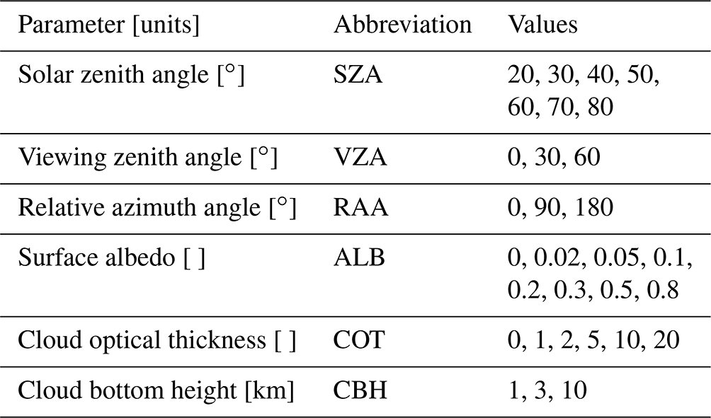
There are three groups of datasets generated by MYSTIC: the first one includes a 1D simulation with a 1 km thick cloud layer for a variety of solar-satellite geometries, surface albedos, and cloud properties as listed in Table 1. This dataset is used to investigate the uncertainty of the NO2 retrieval due to the simplified cloud correction approaches. In addition, clear-sky spectra (COT =0) are calculated for all geometries and surface albedos in order to check the agreement between MYSTIC and VLIDORT RTMs (see Sect. 2.4).
The second dataset includes a simple box cloud with a variety of geometrical and optical thickness. The simulation is performed for a nadir-viewing sensor with a 1×1 km2 field of view (FOV) along a line starting at a distance of 15 km away from the cloud edge in the clear region and ending at a distance of 10 km from the cloud edge in the cloudy scene. This dataset is used to investigate the sensitivity of the NO2 retrieval bias for clear pixels located nearby clouds and to identify the parameters correlated to 3D effects. Furthermore, possible mitigation approaches are investigated using this dataset.
Finally the third dataset includes realistic three-dimensional clouds and typical geometries representative for low Earth orbit (LEO) and geostationary Earth orbit (GEO) satellite observations. The cloud field is taken from the large eddy simulation (LES) based on the ICOsahedral Non–hydrostatic atmosphere model (ICON) (Dipankar et al., 2015; Zängl et al., 2015) for a region including Germany and parts of other surrounding countries. The simulations include all cloud types typical for central Europe. This dataset is used to validate the mitigation approaches described in Sect. 4 below.
2.4 Radiative transfer model settings
Two radiative transfer models are used for the impact assessment of 3D clouds on trace gas retrievals. The synthetic datasets with 3D cloud fields are generated using MYSTIC, whereas the layer-AMFs and modelled reflectances at TOA used for NO2 retrieval and cloud correction are simulated with the linearized vector code VLIDORT (Spurr et al., 2001; Spurr and Christi, 2014, 2019) version 2.7. VLIDORT applies the discrete ordinates method to generate simulated radiances at TOA and analytic derivatives (Jacobians) with respect to atmospheric and surface parameters (i.e. weighting functions). The layer-AMFs ml are derived from altitude-dependent weighting functions determined by VLIDORT:
where I is the simulated TOA radiance, τl is the absorption optical thickness of NO2 at layer l, and the term is the altitude-dependent weighting function for NO2.
We first need to ensure consistency between VLIDORT and MYSTIC; therefore an intercomparison exercise was performed for a 1D plane-parallel clear-sky atmosphere. The simulations from both models use the same atmosphere, including Rayleigh scattering as well as absorption by gases. The comparison of reflectances and layer-AMFs was done for a variety of combinations of solar and viewing geometries and surface albedos as shown in Fig. 1.
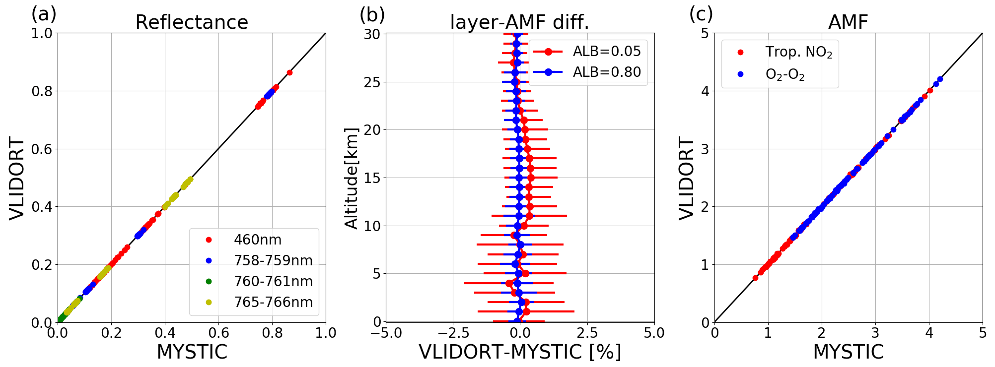
Figure 1Comparison of radiative transfer models (MYSTIC and VLIDORT). (a) TOA reflectance simulated at 460, 758–759, 760–761, and 765–766 nm. (b) Relative difference of layer-AMFs. Red (albedo =0.05) and blue (albedo =0.8) circles with error bars (standard error) are calculated for a variety of geometries. Relative difference between a and b is calculated using % herein. (c) Comparison of AMF calculated with a highly polluted tropospheric NO2 profile (red) and an O2–O2 profile (blue).
Figure 1a compares the reflectance at 460 nm and in three wavelength bands (758–759, 760–761, and 765–766 nm) around the O2–A band for all geometries and surface albedos. The overall differences are 0.0007, 0.0002, 0.0001, and 0.0001 for the above four wavelengths. Corresponding relative differences are generally less than 0.5 %, except for low surface albedo (0.05) at 760–761 nm, where the difference reaches 1 %. Figure 1b shows the comparison of the simulated layer-AMFs at 460 nm for all geometries for surface albedos of 0.05 and 0.8. The averaged difference is within 0.5 % 0.2 % with a standard deviation of 1.8 % 0.7 % for surface albedo . The bias slightly decreases with altitude. The total AMF is calculated from the layer-AMFs by weighting it with two atmospheric absorber profiles: a tropospheric NO2 profile corresponding to a highly polluted case and a O2–O2 profile from the US Standard Atmosphere (Anderson et al., 1986). The tropopause height is set to 15 km in this study. Results are displayed in Fig. 1c. The agreement between the models is good, with average differences of 0.45 % and 0.3 % for NO2 and O2–O2.
In the present work, the main focus is on the effect of 3D clouds. Therefore, radiative transfer model settings in the NO2 and cloud retrievals are made as consistent as possible with those used to generate the synthetic datasets. Although some errors are inevitable, such as those related to differences between MYSTIC and VLIDORT, or due to interpolation in the LUTs, these errors are generally small. We are therefore confident that the differences between retrieved NO2 values and truth (as imposed in the synthetic data) mainly come from the simplified cloud correction approach used in the calculation of the AMF and from 3D cloud effects.
In addition, for very low cloud fraction cases (CFr<1 %), the cloud top height output is highly unstable, and a small difference between the RTMs will lead to a large uncertainty in the cloud height retrieval. Therefore, it is reasonable to consider the observation with CFr<1 % as a clear-sky pixel (i.e. CFw is set 0 in Eq. 2) in order to avoid unnecessary error propagation through the retrievals, which can be as high as 10 %. Moreover, the cloudy scenes (CFw>50 %) are usually excluded in the analysis.
2.5 NO2 retrieval for 1D clouds
In this section, we assess the order of magnitude of the uncertainty that is inherent to conventional cloud correction schemes. We use this uncertainty in order to put in perspective the errors due to the simplistic treatment of clouds for scenes with complex 3D clouds. Two conventional cloud correction schemes are considered here, including FRESCO and the O2–O2 cloud correction scheme. The uncertainty inherent to these schemes is assessed for synthetic scenes with known 1D clouds, considering the deviation of air mass factor obtained by these schemes from the synthetic truth (obtained by MYSTIC), and the difference in the air mass factors between the two schemes.
The retrieval algorithm is applied to synthetic data for 1D cloud scenes with the selected SZAs (30, 60∘), VZAs (0, 30, 60∘), RAAs (0, 90, 180∘), ALBs (0.05, 0.1, 0.3), and various cloud parameters – 1 km thick cloud with CBH of km and COT of . Examples of cloud and NO2 retrievals are shown in Fig. A1. The O2–O2 and FRESCO cloud fraction retrievals show very good agreement. However, cloud pressure retrievals show large differences, especially for high cloud cases. It should be noted that the cloud pressure retrievals based on O2–O2 or O2 absorption must be interpreted as effective values. Furthermore, a more accurate cloud retrieval does not always correspond to a better cloud correction in the NO2 retrieval. For instance, the O2–O2 cloud pressures substantially differ from true values for the high cloud cases, whereas FRESCO cloud pressures are usually compared to the middle of the cloud layer. On the other hand, NO2 AMFs using an O2–O2 correction are often closer to the true AMF than those using FRESCO correction. These results also show different impact on the retrieval between the polluted and clean cases. It implies that the accuracy of the cloud correction relies not only on the accuracy of the cloud retrieval, but also on other factors, such as the NO2 profile.
The error of the NO2 retrieval is evaluated by comparing the calculated AMF with the true AMF, which is calculated using layer-AMFs from MYSTIC (see the companion paper by Emde et al., 2022) combined with the NO2 profile. Figure 2 compares the bias of the NO2 AMF retrieval corrected by cloud parameters derived from the FRESCO and O2–O2 algorithms. The retrievals are applied for polluted and clean NO2 profiles, both taken from the CAMELOT study (Levelt et al., 2009). Retrievals for COT >5 are not shown in the figure, since the corresponding CFws are larger than 50 %, and the cloudy pixels are excluded from the analysis.
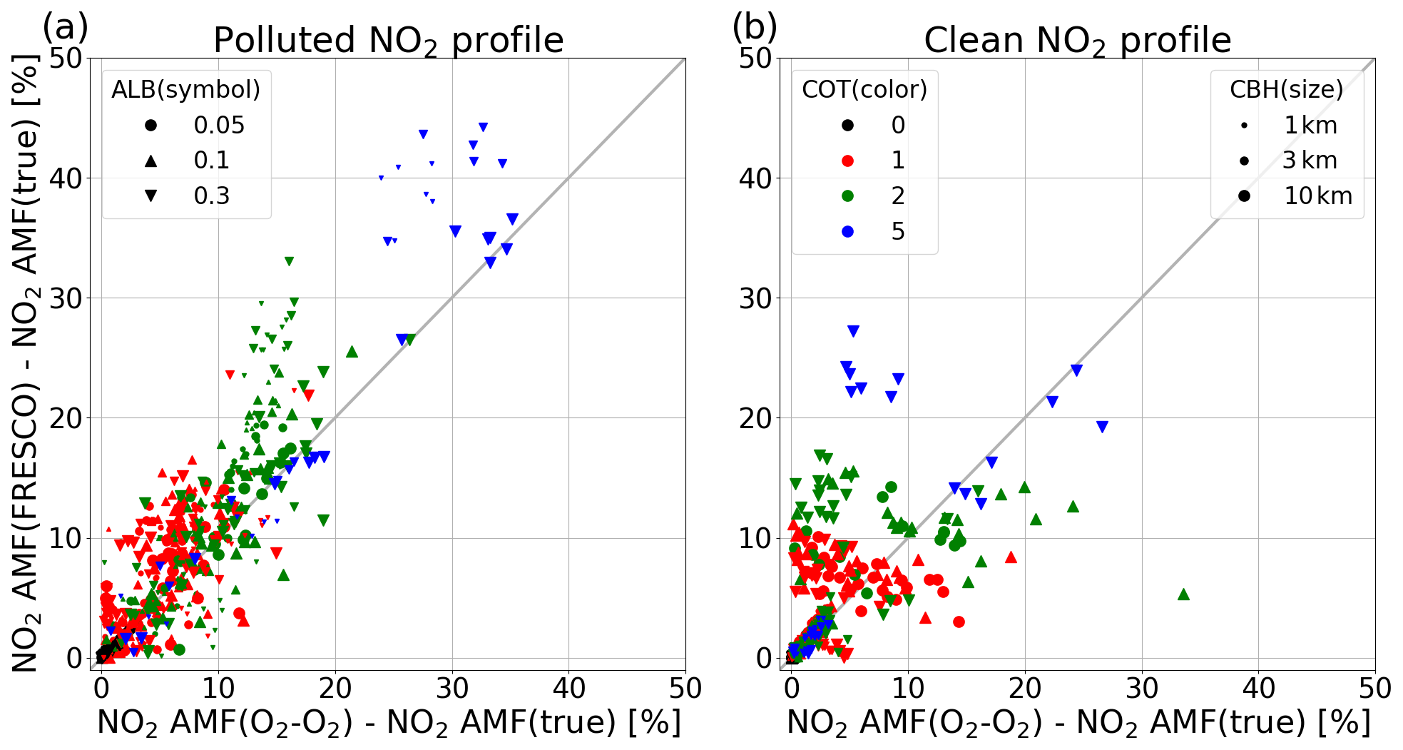
Figure 2Comparison of bias of NO2 AMF retrieval using the cloud correction based on O2–O2 and FRESCO clouds. The retrievals are based on (a) the European polluted and (b) the clean atmospheric NO2 profile, and the retrievals are applied when CFw≤50 %. A variety of symbols, colours, and marker size represent the cases with the different surface albedo, cloud optical thickness, and cloud bottom height.
The NO2 AMF retrieval using FRESCO and O2–O2 cloud corrections generally shows a good agreement, and differences mostly are within 10 %; see Fig. 2. For the polluted cases (Fig. 2a), the bias of the NO2 retrieval is mostly within 20 %. Some higher biases occur for pixels with a high surface albedo (0.3). We also observe that retrieval biases obtained using the FRESCO cloud correction are systematically higher than those obtained using the O2–O2 cloud correction. For clean conditions (Fig. 2b), the retrieval generally shows a lower bias, except a few cases for high clouds (CBH =10 km).
In this study, the calculation of NO2 AMFs assumes perfect knowledge of all parameters, and in particular, the NO2 profile is assumed to be the same inside and outside of the cloud. The error of the NO2 retrieval is mainly from the cloud correction. The bias of the NO2 retrieval using the classic cloud correction schemes is generally lower than 20 %. Therefore, this value is used as a reference amplitude to define the significance of 3D effects in the study.
3.1 Sensitivity study
In reality, the cloud-affected scenes are usually complex; many cloud effects come together that are difficult to distinguish. Moreover, the NO2 retrieval of our interest is a (nearly) cloud-free scene. In order to investigate the influence of the different 3D cloud effects on NO2 retrievals, we start with simple box-cloud cases and investigate the NO2 retrievals for the clear pixels around the clouds. Emde et al. (2022) performed MYSTIC radiative transfer simulations with a box cloud. The simulations are made for an imaginary nadir-viewing sensor with a 1×1 km2 FOV, and two types of cloud base cases are defined to represent a low-altitude liquid cloud (2-3 km) and a high-altitude ice cloud (9-10 km). In addition, the scenarios include a variety of solar zenith angles, surface albedos, cloud optical thickness, cloud geometric thickness (CGT), and cloud bottom heights.
The standard NO2 retrievals based on both O2–O2 and FRESCO cloud algorithms are applied to the synthetic spectra for a polluted case, and the impact of 3D effects is identified on clear-sky pixels by comparing AMF values from the retrieval with corresponding true values. Figure 3 shows the bias of the NO2 AMF retrieval due to cloud in-scattering and shadowing. In the in-scattering region (Fig. 3a), a negative or positive bias is observed for a few pixels next to the cloud edge. For these pixels, the retrieved CFr is greater than 0 due to the enhanced reflectance, and the O2–O2 value is slightly larger than that of FRESCO. Cloud pressure retrieval is usually a bit lower than surface pressure but higher than neighbouring cloud pressure, and the FRESCO cloud pressure is relatively higher (not shown). Although there are some differences between the retrievals using O2–O2 and FRESCO cloud corrections, the biases are generally small. In the cloud shadow region, the reflectance is lower than the clear-sky reflectance. Accordingly, the retrieved CFr is 0, and the calculated AMF corresponds to the clear-sky AMF. Since the true AMF is generally smaller than the clear-sky AMF in the cloud shadow, the retrieved AMF tends to be overestimated (see Fig. 3b), and these differences can reach up to 125 % depending on the SZA, cloud height, and distance from the cloud edge. Outside of the cloud shadow region, a small retrieval bias remains, especially for the low cloud cases, which is due to an effect of horizontal scattering from the cloud edge (namely, channelling effect). The retrieval biases are generally small for a clean profile as shown in Fig. A2 except for the high cloud cases with SZA equal to 80∘.
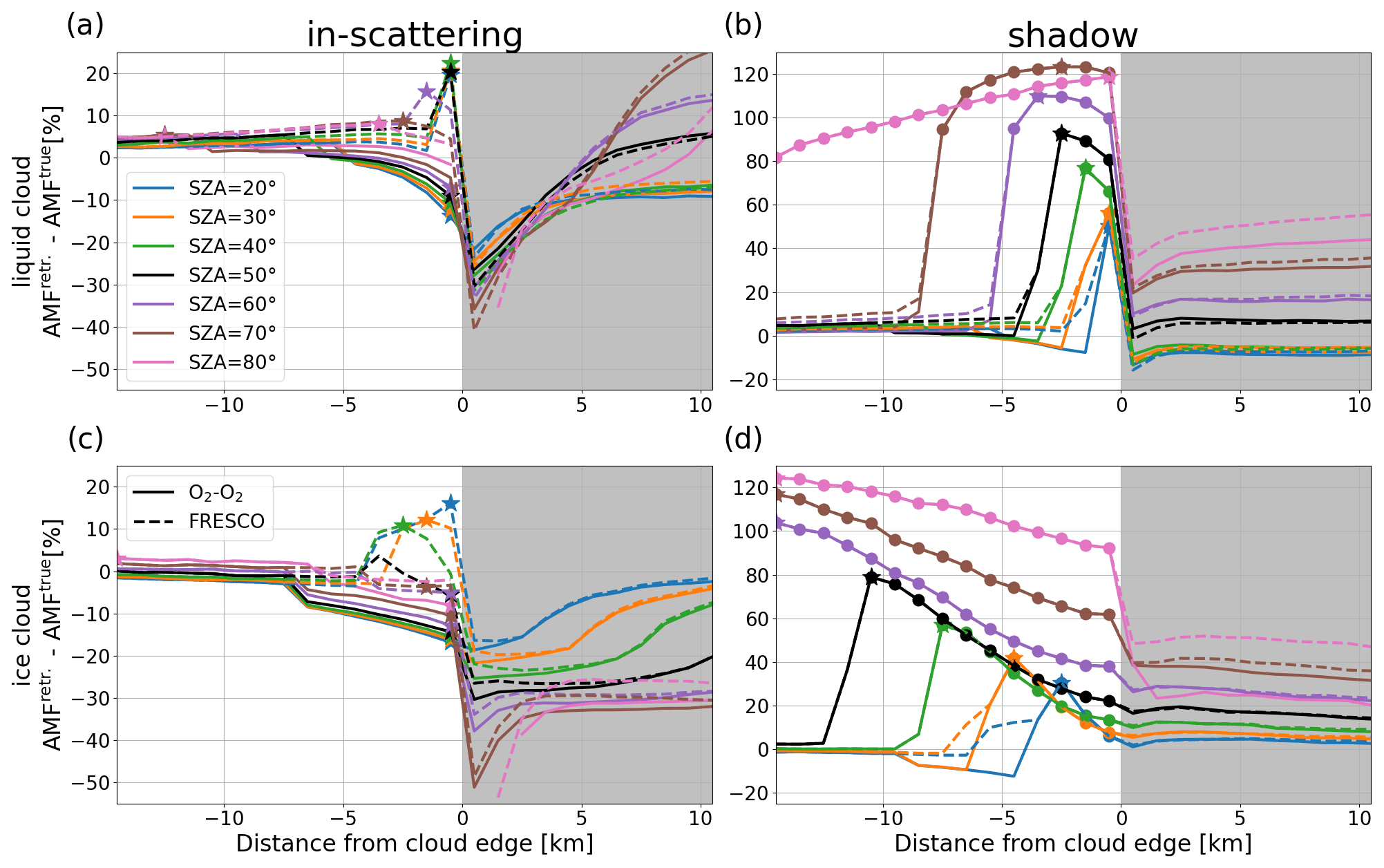
Figure 3NO2 AMF retrieval bias as a function of the distance from the cloud edge for the different SZAs. Negative distances from the cloud edge correspond to the pixels in the clear region (white regions), and positive distances correspond to the pixels in the cloudy region of the domain (grey regions). Panels (a) and (b) are for the low cloud, and panels (c) and (d) are for the high cloud. Panels (a) and (c) show cloud in-scattering, and panels (b) and (d) show cloud shadow. Solid and dashed lines correspond to retrievals corrected by O2–O2 and FRESCO cloud algorithms, respectively. Stars correspond to the largest absolute bias over the clear region for each scenario, and dots in the cloud shadow region (b, d) denote the horizontal extent of the cloud shadow.
Although cloudy pixels are not our primary focus here, it is interesting to note that retrieval biases for such pixels depend on the distance from the cloud edge and imply the effect of 3D clouds. Note also that we obtain very good agreement between the retrievals corrected by the two cloud approaches, and only a slightly larger difference (10 %) occurs for SZA =80∘ in the cloud shadow cases.
3.2 Identification of conditions leading to the largest biases
In order to study the dependence of the NO2 AMF bias due to the cloud shadowing/in-scattering for the parameters defined in the previous section, the largest absolute retrieval bias over the clear region is selected for each scenario and is plotted as a function of various parameters. The retrieval includes the O2–O2 and FRESCO cloud correction, and the results are shown in Fig. 4.
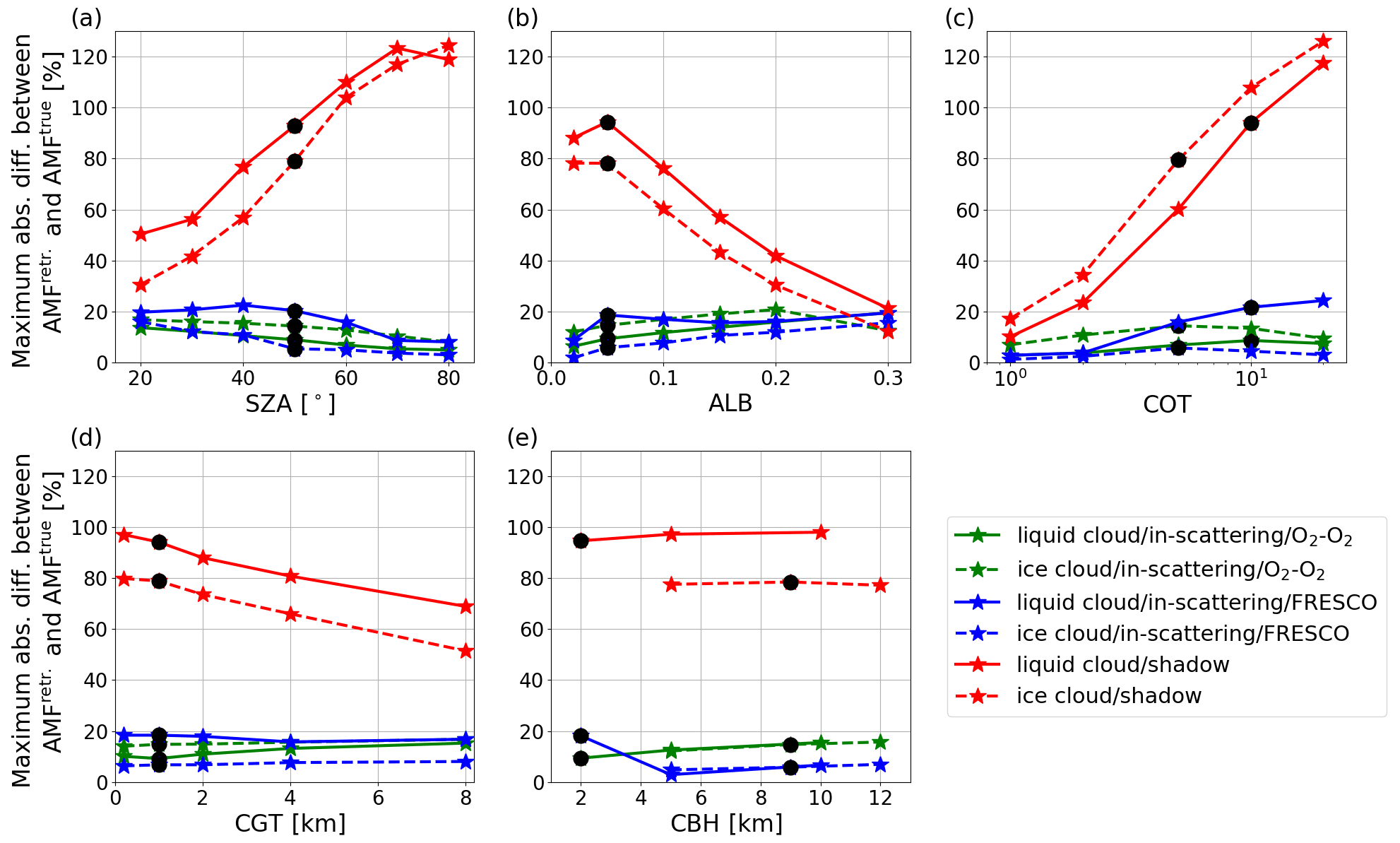
Figure 4Maximum NO2 AMF bias for the polluted NO2 profile in the clear regions as a function of solar zenith angle (a), surface albedo (b), cloud optical thickness (c), cloud geometric thickness (d), and cloud bottom height (e). Solid and dashed lines represent the retrieval for the simulations with liquid and ice water clouds respectively. The green and blue lines depict the AMF biases using O2–O2 and FRESCO cloud corrections over the in-scattering region, and the red lines correspond to the retrieval bias in the cloud shadow. Black dots refer to the base cases (SZA =50∘, ALB =0.05, COT , CGT =1 km, CBH km for liquid/ice cloud), which are defined in Sect. 3.1 of Emde et al. (2022).
In the cloud shadow cases, the retrieved CFr is 0, and therefore the NO2 retrieval does not correct for the presence of clouds. The impact of the cloud shadow strongly depends on the SZA, ALB, and COT. Related biases increase from ∼40 % for SZA =20∘ to more than 100 % at high SZA (>60∘) and from 10 % for COT =0.2 to 120 % for COT =20. They decrease from 80 % to 90 % for ALB =0.02 to 20 % for a higher albedo value (0.3). Increased surface albedos increase the reflection from the ground, which compensates for the reduced transmission of sunlight in the cloud shadow and thus reduces relative biases. The dependence of the bias on CGT is relatively small within the range of 50 % and 100 %, and the impact marginally depends on CBH. In the cloud in-scattering regions, the retrieval biases are much smaller. The retrieval AMFs corrected by O2–O2, and FRESCO cloud algorithms display biases of up to 25 % for all cases. The same analysis was conducted for a clean NO2 profile as shown in Fig. A3. In this case, biases are overall small and mostly within 20 %. Thus, in the following, we will concentrate on the retrievals in the cloud shadow region for polluted conditions, which give the largest 3D-related biases.
3.3 Influence of the NO2 vertical profile
In order to investigate the effect of the NO2 profile on the retrieval, two model profiles with maxima at different heights are used. The box profile has a constant NO2 concentration below the given height, while for the triangle profile, the NO2 concentration decreases linearly with altitude, and the value above the given height is 0. Figure 5 shows examples of the box and triangle model profiles with a height of 3 km, as well as the polluted and clean profiles used in the study. The profiles are normalized by the tropospheric columns. They are used to calculate both retrieval and true AMFs, for the cases corresponding to box clouds at different altitudes. The largest retrieval bias of each case is selected as a function of the model profile height and displayed in Fig. 5b.
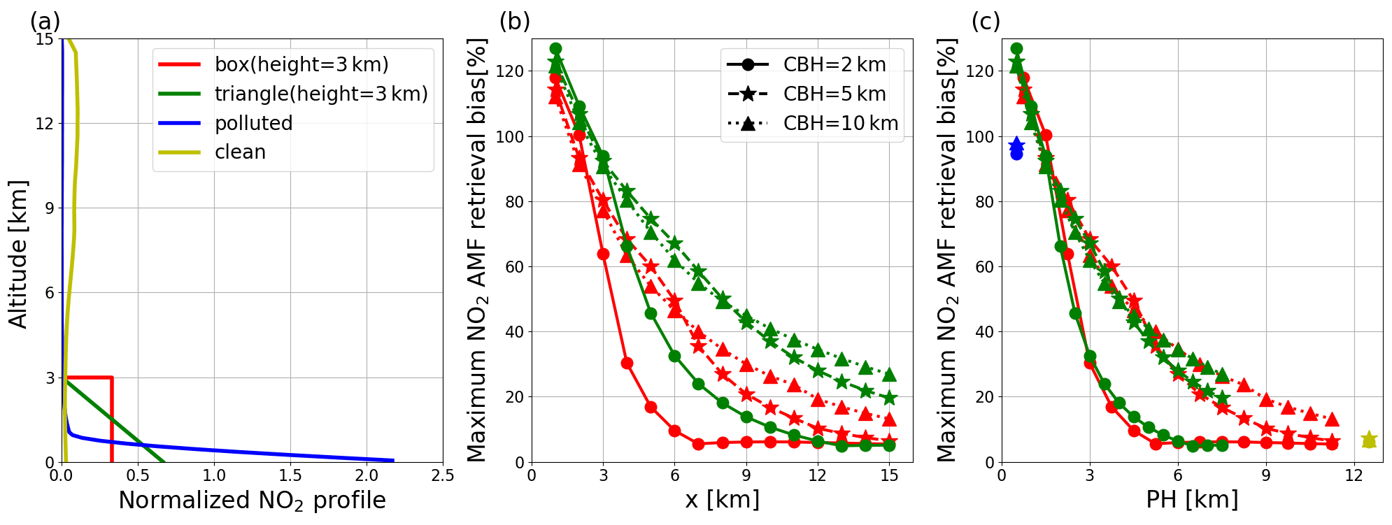
Figure 5Dependence on NO2 profile shape of the NO2 AMF bias in the cloud shadow. (a) Selected NO2 profile shapes. (b) Largest AMF retrieval biases for the cases with liquid water cloud at different altitudes, as a function of the model height. Panel (c) similar to panel (b) but as a function of the profile height parameter. See text for further details.
In order to describe the shape of the NO2 profile, we introduce a parameter: the profile height, i.e. the altitude (pressure) below which resides 75 % of the integrated tropospheric NO2 profile. For example, the profile height for 3 km box and triangle profiles is 2.25 and 1.5 km, respectively. The bias of the NO2 retrieval for both profile shapes shows a consistent dependency on profile height (Fig. 5c). The profile height for the polluted and the clean NO2 profile is 0.5 and 12.5 km, respectively, and the corresponding NO2 retrieval biases are 95 % and 6 %. Note that the retrieval bias for the polluted NO2 profile (blue points) is 20 %–30 % lower than for the 1 km box profile, while both profiles share the same profile height. This may link to other factors not considered here, such as the cloud top height. Generally speaking, 3D effects will increase the layer-AMF above the clouds and decrease it below the clouds (see Fig. 6 of Emde et al., 2022). Because of such compensating effects, the presence of NO2 above the cloud will reduce the bias in the AMF calculation for the polluted profile.
3.4 Change of spatial resolution
The 3D cloud effects depend on the spatial resolution of the satellite measurements. The synthetic data with a box cloud used in this study correspond to a resolution of 1×1 km2, while the spatial scales of TROPOMI (3.5×7 km2 at nadir, 3.5×5.5 km2 since 6 August 2019), Sentinel-4 (from 9×12 km2 at a reference point at 45∘ N and degrading away from the sub-satellite point), and Sentinel-5 (7.3×7.5 km2 at nadir) are larger. In order to investigate 3D effects at the spatial resolution of the Sentinels, we bin synthetic spectra by a factor of 3, 5, 7, 9, 11, 13, and 15 to represent the measurements with spatial resolutions of 3-15 km. The new spectra are obtained using moving averages of 3–15 pixels, and the true layer-AMFs are calculated using an intensity-weighted average based on the radiance at 460 nm.
The standard retrieval algorithm using the O2–O2 cloud correction is applied to the binned dataset. Figure 6 shows examples of the NO2 retrieval error based on the binned data for a variety of SZAs and for spatial scales of 3, 7, 11, and 15 km. The pixels can be divided into three categories: (1) the dark grey region on the right side is the cloudy scene, (2) the region on the left side is the clear scene, and (3) the light grey area in the middle part corresponds to partly cloudy partly clear scenes. In the clear region, the number of pixels completely in the cloud shadow (denoted by dots) decreases with the increasing pixel size. At 3 km resolution, pixels completely in the cloud shadow can be found for SZA ≥50∘, while such pixels are only found for SZA =80∘ for a pixel size of 15 km. This is linked to the cloud shadow area, which is determined by the cloud top height and SZA. The retrieval bias significantly decreases when the cloud shadow fraction is less than 1 (pixels on the left side of the dots).
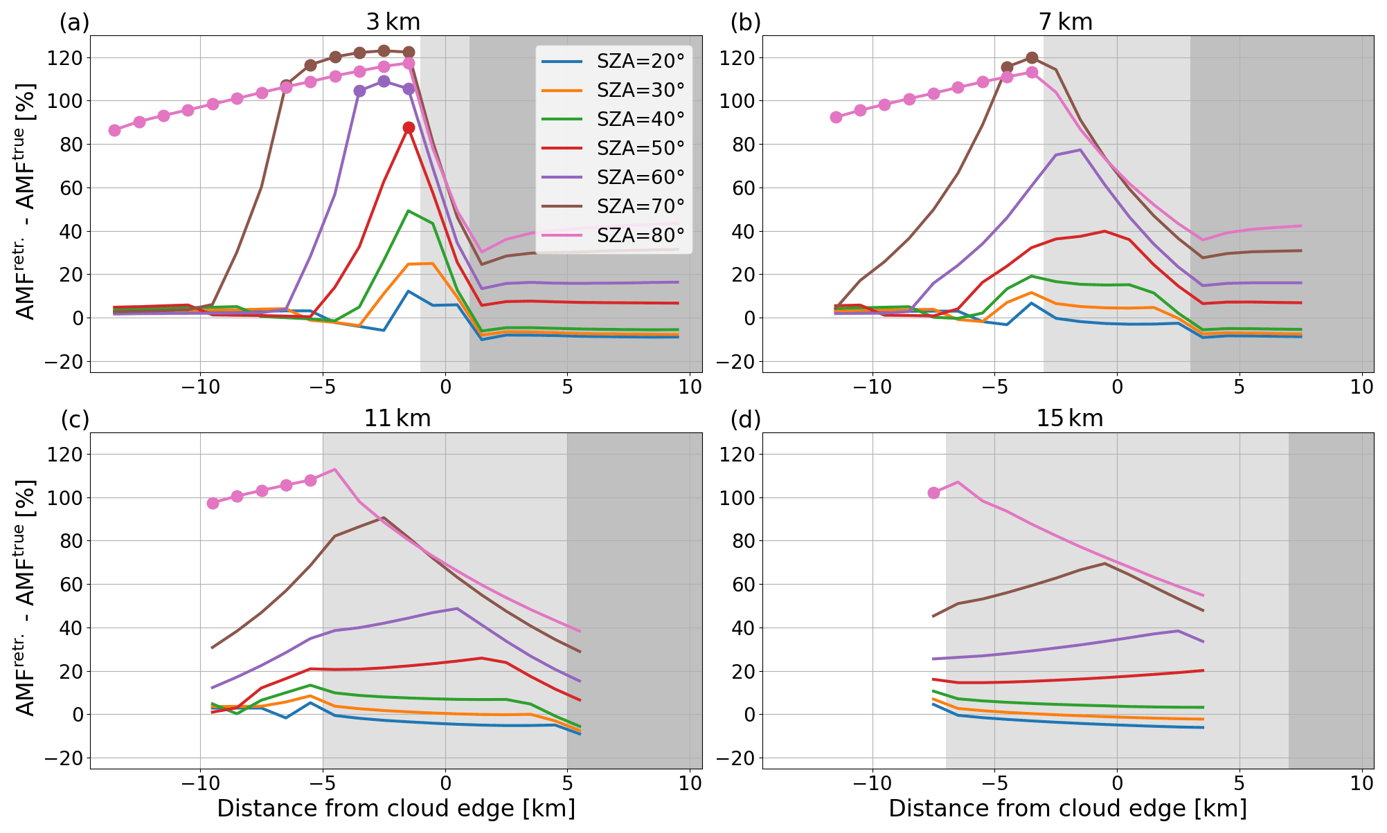
Figure 6Liquid cloud NO2 AMF retrieval bias for box-cloud simulations with spatial resolutions of (a) 3, (b) 7, (c) 11, and (d) 15 km, as a function of the distance from the cloud edge for a variety of SZAs. The dark grey region is fully cloudy, the light grey region partly cloudy, and the white region fully clear. Dots represent conditions where the whole pixel is in the cloud shadow. The AMF uses the O2–O2 cloud correction and is calculated with the polluted NO2 profile.
We apply the standard retrieval algorithm to all binned datasets and extract the same statistics as in Fig. 4. Results are shown in Fig. 7. In general, the retrieval bias decreases with increasing spatial scales due to spatial averaging. The cloud shadow effect strongly depends on the fraction of the pixel that is in the cloud shadow. When the shadow area is smaller than the size of the satellite footprint, the cloud shadow effect will be significantly reduced. Otherwise, the change is relatively small. The cloud shadow area for the low liquid cloud cases is usually less than 15 km, and the AMF retrieval bias significantly decreases with the increasing pixel size, whereas the dependency of the bias on spatial resolution is relatively weak for the high cloud cases, since their cloud shadow area is usually larger than 15 km. Note that the synthetic data used in this study assume that the NO2 column is the same in clear and cloudy regions as well as in cloud shadow. Consequently, the NO2 retrieval is based on the same assumption. In reality, however, the NO2 column usually shows significant to large horizontal variability, which leads to uncertainty in the retrieval. The importance of such effects cannot be easily assessed using tools available for this study and would need to be further investigated.
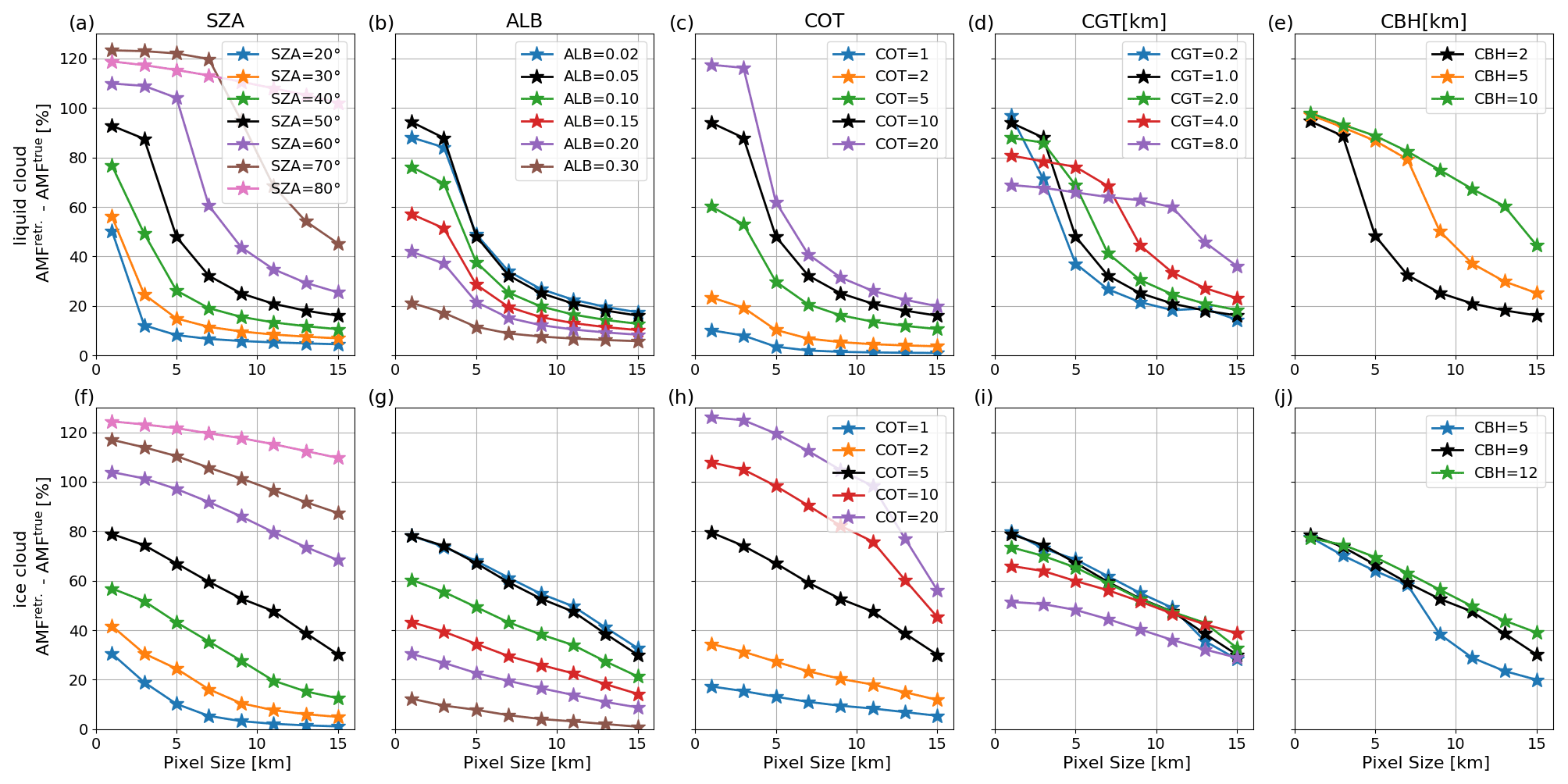
Figure 7Maximum NO2 AMF bias in the cloud shadow as a function of the pixel size for the liquid (2–3 km altitude) and ice clouds (9–10 km altitude) for various values of the SZA, ALB, COT, CGT, and CBH.
3.5 Cloud shadow fraction
As discussed in the previous section, the retrieval bias significantly decreases when the cloud shadow fraction is less than 1. Therefore, the cloud shadow fraction (CSF) is a key parameter to quantify cloud shadow effects. In order to study the relationship between retrieval bias and cloud shadow fraction, we first extract all the pixels in the clear region from the liquid cloud cases for SZAs of 50 and 70∘. Simulations with the different bins are used in the analysis. The cloud shadow fraction is calculated based on the geometric relationship between cloud top height, SZA, and distance from the edge of the cloud. Results are shown in Fig. 8a. Note that the AMF biases and the cloud shadow fractions are nearly linearly dependent.
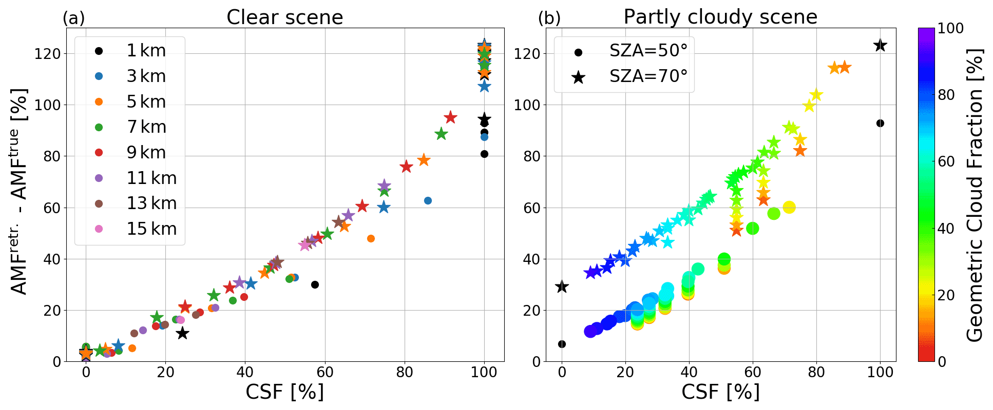
Figure 8NO2 AMF retrieval bias for the liquid cloud cases in the cloud shadow with various spatial resolutions over the clear (a) and the partly cloudy (b) region, depending on cloud shadow fraction. Circles and stars are the cases for SZA =50 and 70∘, respectively. See text for further details.
In addition, a similar analysis (displayed in Fig. 8b) is performed for the partly cloudy region. The colours represent the geometric cloud fraction, and the black points are the averaged retrieval bias in the cloudy and cloud shadow regions. There is an almost linear dependency for most of the pixels. However, some obvious outliers can be found for SZA =70∘ and CSF =0.55, 0.63, and 0.75. This may be linked to the different contributions of cloudy, shadow, and clear sky.
Based on the above discussion, the independent pixel approximation can be used to estimate the retrieval bias. We assume that the bias can be expressed as a linear combination of the bias from the clear-sky, shadow, and cloudy parts, and we apply this approach to the data shown in Fig. 8b. It should be noted that the retrieval bias is negligible for cloud-free pixels since differences between the VLIDORT and MYSTIC models are very small (see Sect. 2.4). Therefore, the retrieval bias is set to 0 for clear-sky scenes. Results are shown in Fig. 9. As can be seen, there is a good general agreement between the true bias and the estimated one.
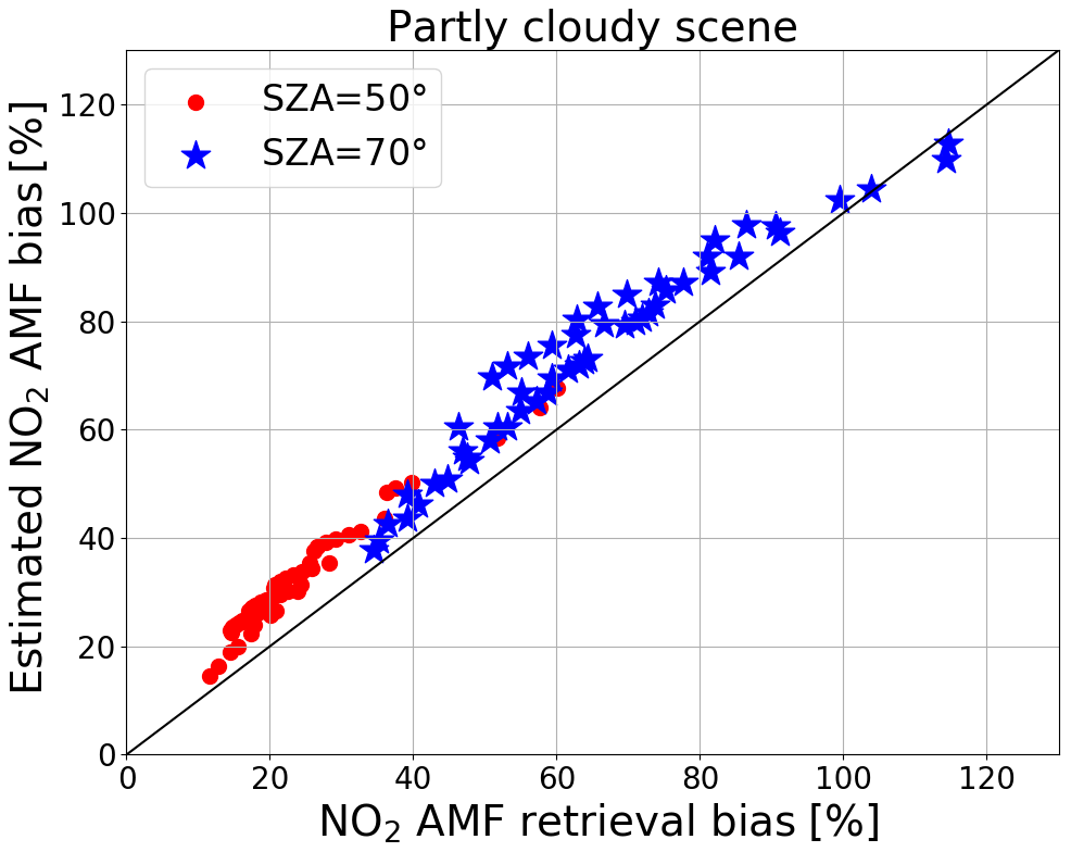
Figure 9Estimated vs. true AMF retrieval bias for partly cloudy scenes. The estimation is based on a linear combination of the AMF retrieval bias over clear, cloud shadow, and cloudy scenes. See text for further explanations.
3.6 Dependence on slant cloud optical thickness
We introduce the slant cloud optical thickness (SCOT), which corresponds to the integrated extinction of the cloud from the Sun through the atmosphere to the ground along the line of sight. The SCOT can be used to judge whether a ground pixel is in the cloud shadow. For the box-cloud cases, the SCOT for the pixels in the cloud shadow is calculated as SCOT . As we can see in Fig. 4, the NO2 bias strongly depends on SZA and COT, which are both linked to the SCOT.
In Fig. 10a, the averaged retrieval bias is calculated over the cloud shadow region for each case as a function of SCOT. There is a quasi-linear relation between the bias and the logarithm of the SCOT. The analysis is also done for the synthetic data with the LES clouds. Simulations for nadir observations (VZA =0∘), a variety of SZAs (20, 40, and 60∘), and surface albedo of 0.05 are used. The SCOT is calculated from the direct transmittance using MYSTIC based on the synthetic input of 3D fields of the cloud optical thickness from ICON. This approach is the same as for the calculation of the cloud shadow index, which is described in Sect. 3.3 of Kylling et al. (2022). Figure 10b shows the AMF retrieval bias as a function of the SCOT. Again, only the nearly cloud-free pixels are used (CFw<50 %). The retrieval error is close to 0 when SCOT <1 and significantly increases for SCOT >1.
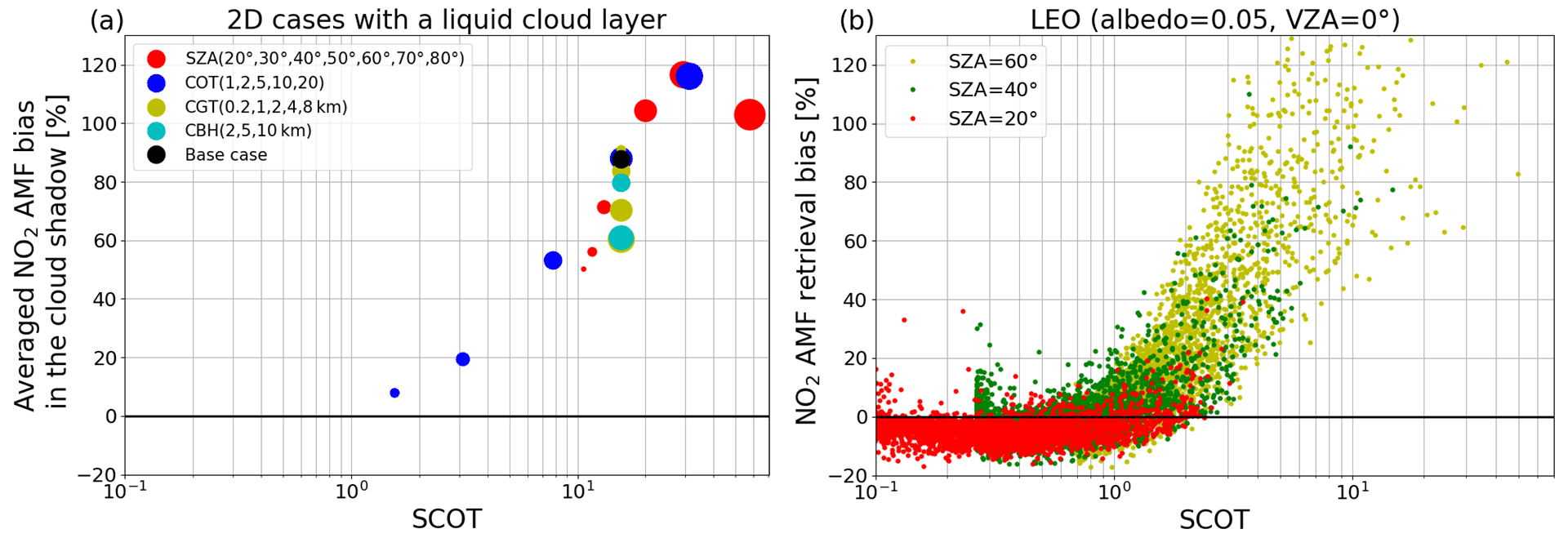
Figure 10NO2 AMF retrieval bias as a function of slant cloud optical thickness. (a) Box-cloud cases with the liquid cloud. The bias is averaged over all the pixels in the cloud shadow, and the various colours and marker sizes represent cases with different solar zenith angles, cloud optical thicknesses, cloud geometric thicknesses, and cloud bottom heights. (b) Synthetic data with LES clouds for low Earth orbit (LEO) satellite geometries (VZA =0∘, SZA =20, 40, and 60∘) and a surface albedo of 0.05. The black line shows the bin average with standard deviations (error bars). Only retrievals with CFw<50 % are used.
4.1 Approaches
In this section, various approaches to mitigate biases due to the cloud shadows are explored. These include (1) calculation of the AMF using an effective isotropic surface albedo that is fitted based on the observed TOA Earth radiance; (2) correction of the NO2 retrieval using the deviation of the retrieved O2–O2 SCDs and the reference calculations for a clear scene under the same geometry and surface albedo; and (3) estimation of the NO2 bias using an empirical formula which parameterizes the bias as a function of driving parameters including the cloud shadow fraction, SCOT, NO2 profile height, and cloud top height.
4.1.1 NO2 AMF using extended cloud retrievals
For pixels in the cloud shadow, the standard NO2 retrieval will treat the scene as cloud-free when the measured radiance is smaller than the corresponding clear-sky radiance. For such pixels, cloud correction is not applied in the AMF calculation. The current cloud algorithms can in fact deal with such situations if the retrieval is extended such that negative cloud fractions are allowed. Figure 11 shows examples of extended O2–O2 (a) and FRESCO (c) cloud retrievals and corresponding NO2 AMFs. In the cloud shadow regions, both CFr values are negative. The FRESCO CFr is slightly smaller than the O2–O2 one, while the FRESCO cloud pressure is higher than the O2–O2 one. In addition, the retrieved cloud pressure in the cloud shadow area is higher than the cloud pressure from the neighbouring cloud pixels. The bias of the NO2 AMF using the extended O2–O2 cloud is higher than the bias based on the standard approach, whereas this bias is significantly reduced when the AMF calculation uses the extended FRESCO cloud.
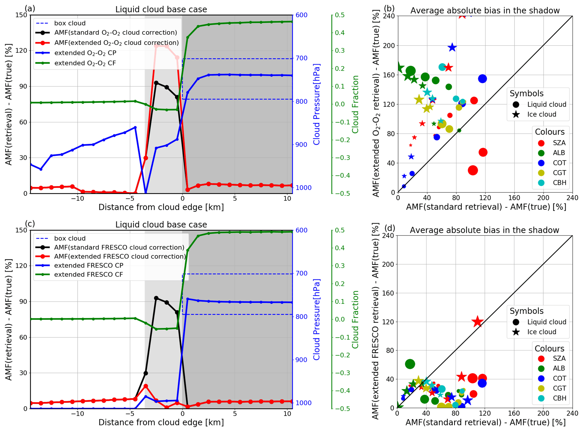
Figure 11Examples of NO2 AMF retrieval using the extended O2–O2 (a, b) and FRESCO (c, d) cloud. (a, c) Comparison of the AMF biases based on the standard retrieval approach and the AMF calculated with the extended cloud retrievals for liquid cloud base case. The dark grey, light grey, and white regions represent cloudy, cloud shadow, and clear scenes, respectively. (b, d) Comparison of the AMF biases for the simulations with a box cloud. Each point represents the average bias in the cloud shadow, and colours correspond to various parameters for the cases with the liquid cloud (circles) and ice cloud (stars). The biases are shown in relative values, and the various marker sizes represent different parameter values.
In order to further verify these correction approaches, we applied the cloud and NO2 retrievals to the various box-cloud scenarios discussed in Sect. 3, and corresponding results are shown in Fig. 11b and d. In the cloud shadow regions, the retrieval biases are even higher than the standard retrieval bias when the correction uses the extended O2–O2 retrieval; however they are mostly reduced for the retrievals based on the extended FRESCO retrieval. Note that the retrieved cloud pressure is close to the surface pressure in the cloud shadows, and the NO2 retrieval for polluted conditions is very sensitive to the cloud pressure retrieval. The cloud pressure differences between both cloud algorithms are usually less than 100 hPa (not shown), and this leads to a change in AMF by more than a factor of 2.
Another possible extension of the cloud retrieval algorithm is to use a more realistic cloud treatment, such as the clouds-as-layers (CAL) approach, which treats the cloud as a uniform layer of light-scattering water droplets, instead of a Lambertian cloud model. This approach has been used to investigate the NO2 retrieval from GOME-2 based on the OCRA/ROCINN cloud retrieval (Liu et al., 2020, 2021). However, OCRA/ROCINN uses a sophisticated approach (Loyola et al., 2018), and to develop such a cloud retrieval algorithm is beyond the purpose of this study. Instead, a simple approach is applied, which assumes that the cloudy scenes are 100 % covered by a uniform layer of water cloud with a 1 km geometrical thickness. The cloud single scattering albedo is set as 1, and the asymmetry parameter is assumed to be 0.85. These values are consistent with those used in the cloud and NO2 retrieval (Liu et al., 2020, 2021). The cloud correction in the NO2 retrieval uses the same cloud properties as the cloud retrieval. This approach retrieves cloud top pressure and optical thickness based on measured reflectances at 460 nm and O2–O2 SCD or three 1 nm (758–759, 760–761, and 765–766 nm) averaged radiances around the O2–A band. In addition, negative cloud optical thicknesses are allowed by using extrapolation in the retrieval in order to treat the cloud shadow situations.
Examples of CAL cloud retrievals are shown in Fig. 12a and c. In the cloudy scene, the cloud optical thickness retrieval is around 8, and the cloud top pressure is slightly higher than 700hPa, which is close to the true value. There is a small difference between the retrievals from the O2–O2 and O2–A band. The bias of the NO2 AMF using the CAL cloud is slightly smaller than the bias based on the Lambertian cloud correction. In the shadow, the retrieved cloud optical thicknesses are negative, and the value from the O2–A retrieval is slightly smaller. The cloud top pressure is higher in the shadow than in the neighbouring cloudy pixels. The bias of the NO2 retrieval using the O2–O2 and O2–A CAL clouds is slightly different from the bias using the Lambertian cloud correction. In general, there is a good agreement between the NO2 retrievals using the CAL and Lambertian cloud models, and the biases of the retrieval corrected by the CAL cloud are slightly higher than those based on the Lambertian cloud correction (Fig. 12b and d).
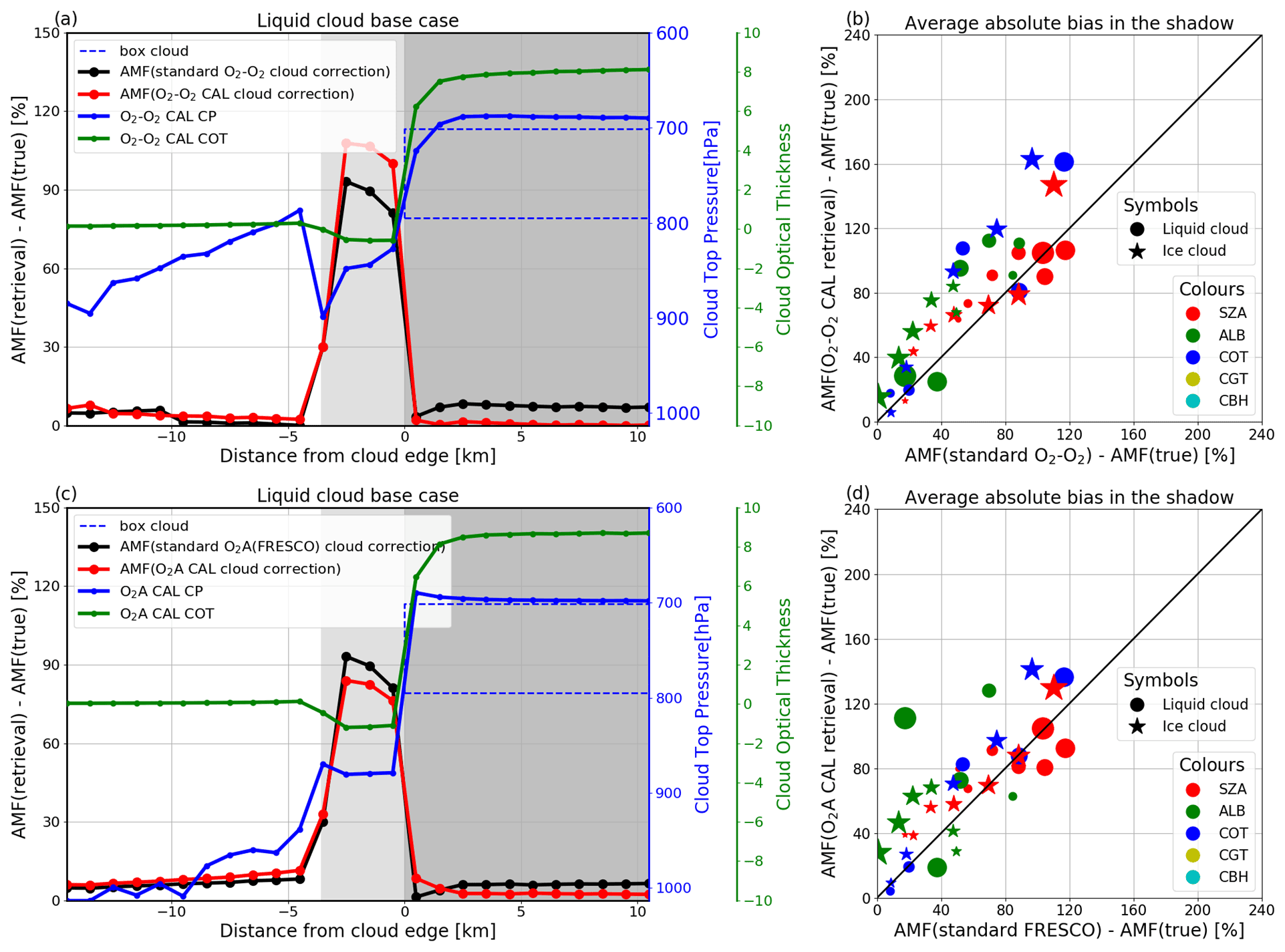
Figure 12Similar to Fig. 11, but the NO2 retrieval uses cloud correction based on a clouds-as-layers approach. Cloud pressures given on the right of panels (a) and (c) are cloud top pressures. In (b) and (d), the x axis on the right represents the retrieval bias based on the NO2 retrieval using the standard O2–O2 (b) and FRESCO (d) clouds, respectively.
4.1.2 NO2 AMF using fitted surface albedo
In the cloud shadow, the standard NO2 retrieval algorithm, which uses a known surface albedo, has a positive bias in the retrieved AMF, whereas the TOA reflectance shows a negative bias compared to the corresponding clear-sky reflectance (Fig. 13a). In an attempt to compensate for such a positive bias, we calculate the AMF using an effective surface albedo based on the measured reflectance. The surface is assumed to be a Lambertian reflector, and the surface albedo is obtained by fitting the simulated reflectance at TOA in a pure Rayleigh scattering atmosphere under a cloud-free condition. The retrieved albedo is then used for the NO2 AMF retrieval. Figure 13a shows that the bias of the retrieval based on AMFs calculated using an effective albedo is significantly reduced in the cloud shadow. However the correction approach tends to increase the retrieval bias for clear-sky pixels outside of the cloud shadow, and for the cloudy region, the retrieval bias based on the effective albedo is much larger than using the standard approach.
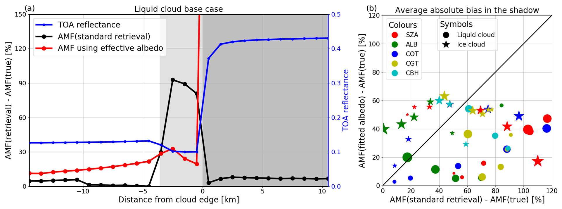
Figure 13Similar to Fig. 11 but for the NO2 AMF using the effective surface albedo. Notice that the x and y range in panel (b) is [0,120] instead of [0,240].
In order to verify the feasibility of the correction approach, we compare the biases of the NO2 retrieval for the standard retrieval approach and calculations based on a fitted surface albedo for various box-cloud scenarios, as shown in Fig. 13b. As can be seen, the retrieval is improved for most of cases; however higher biases are found for high cloud cases (shown as stars in the figure). Further investigations indicate that the retrieved surface albedo is 0 for these pixels, which introduces a large negative error in the AMF calculation. It should be noted that the retrieved albedo value is restricted between 0 and 1. Therefore, the measured radiance for such pixels is smaller than or equal to the corresponding radiance, with an albedo of 0 for clear-sky condition. This correction can be extended to satellite measurements where the fitted surface albedo is lower than climatological values, which may reduce retrieval errors due to surface albedo uncertainties. However, the surface albedo at the UV–visible wavelengths is usually small. Since the NO2 AMF calculation is very sensitive to surface albedo, especially for low surface albedo and polluted regions (Boersma et al., 2004), such cases can cause significant error in the NO2 retrieval.
4.1.3 AMF scaling by O2–O2 SCD
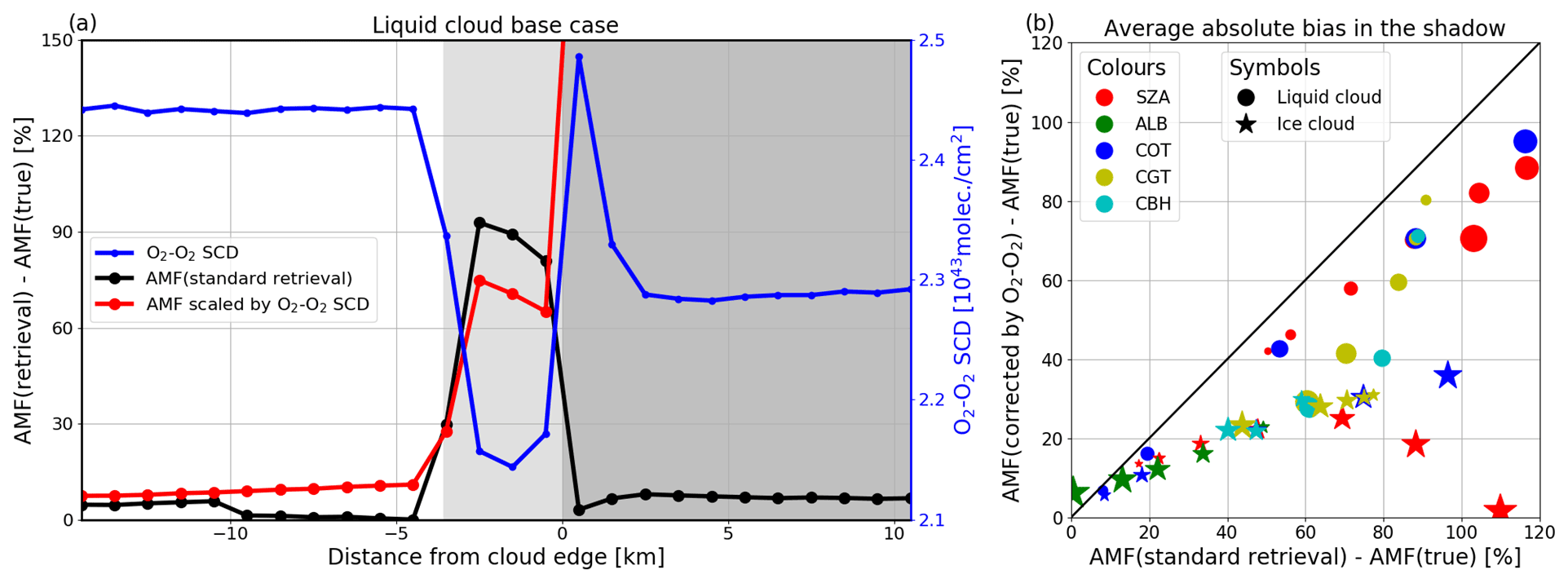
An alternative approach to correct the NO2 retrieval in the cloud shadow is to use the difference between the retrieved O2–O2 SCDs and the reference calculations for a clear scene under the same condition:
where and are the NO2 AMF and the O2–O2 SCD calculated for the clear scene, and is the O2–O2 SCD derived from the observed spectrum. In the cloud shadow regions, the retrieved cloud fraction is 0 since the measured reflectance is smaller than the corresponding clear-sky reflectance. As a result, the AMF in the retrieval is the clear-sky AMF. The basic idea of this correction approach relies on the assumption that there is a certain degree of similarity between the O2–O2 and polluted NO2 profiles, since both species have highest concentration near the surface. However since profiles are not identical, the method can only partly correct for cloud shadow effects. Figure 14 shows a clear negative correlation between O2–O2 SCD and the standard retrieval bias. After applying the correction using Eq. (8), the biases are reduced by about 20 % in the shadow. Again, this approach is not suitable for the cloudy pixels. For the synthetic box-cloud cases, the retrieval bias is systematically reduced when the correction approach is used. The improvement is 10 %–30 % for the low cloud cases and is more noticeable for the high cloud cases.
4.1.4 Parameterization approach
Following the discussion in Sect. 3, the error of the NO2 retrieval in the cloud shadow depends on the cloud shadow fraction, slant cloud optical thickness, NO2 profile, neighbouring pixel cloud top height, and surface albedo, as well as the solar-satellite geometries. Ideally, the 3D bias can be quantified as a function of the above parameters and stored in the LUT. However, there is a limited number of synthetic datasets due to the limited computational resources. Based on the current dataset, an exercise can be done for the condition with a nadir view (VZA =0∘) and a surface albedo of 0.05. In such conditions, the bias of the NO2 retrieval due to cloud shadow effects can be described as
where PH is the NO2 profile height, NCTH is the cloud top height of the neighbouring pixel, log (SCOT) is the logarithm of slant cloud optical thickness, and CSF is the cloud shadow fraction.
F1, F2, and F3 are all quadratic polynomials, and the coefficients of the polynomial are obtained by fitting the averaged NO2 AMF bias in the cloud shadow from a series of simulations with a box cloud as presented in Sect. 3. The cases with a cloud shadow area larger than 16 km are excluded from the analysis (e.g. SZA =80∘ for low cloud and SZA =70∘, 80∘ or CBH =12 km for high cloud) since the synthetic data only simulate the spectra 0–15 km away from the cloud edge. We obtain the following results:
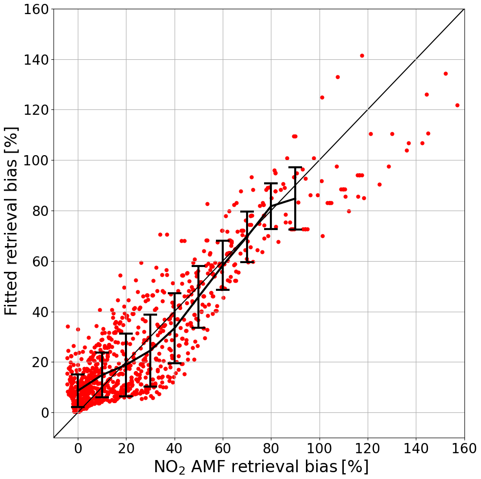
As can be seen in Fig. 15, the difference between the parameterization estimation and the true bias is mostly within 20 %.
4.2 Comparison of mitigation strategies for synthetic data
We applied the correction approaches described in previous sections to NO2 retrievals applied to synthetic dataset with realistic LES clouds. Figure 16 compares AMF biases obtained using the correction approaches described in Sect. 4.1.1, 4.1.2, and 4.1.3 with retrieval biases from the standard algorithm.
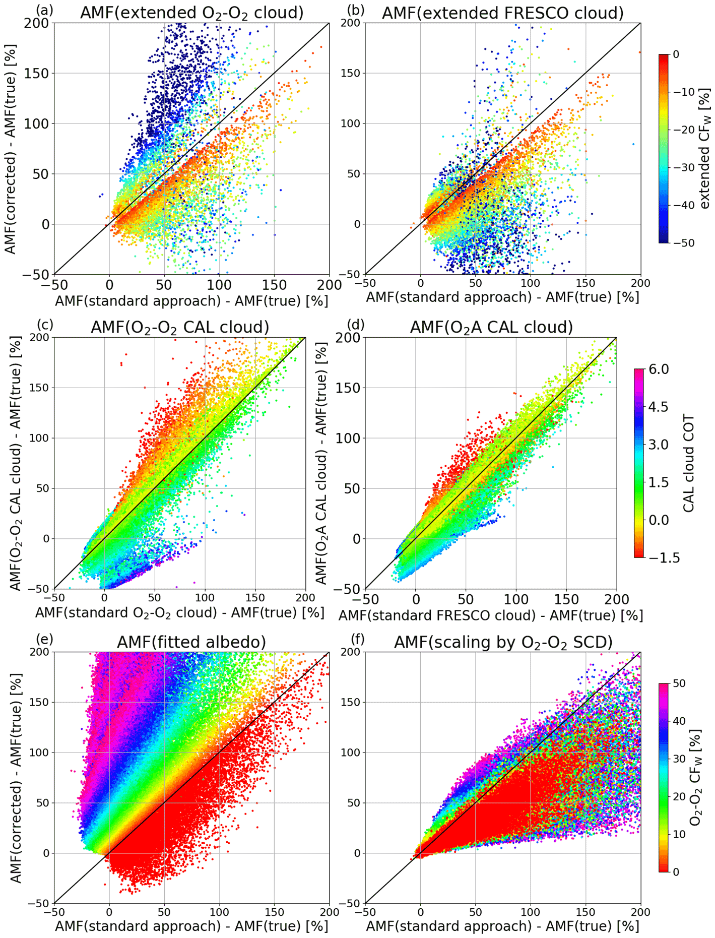
Figure 16Comparison of the AMF bias using the standard retrieval algorithm and three correction approaches for the synthetic data with realistic LES clouds. Panels (a)–(d) show the AMF calculation based on the extended cloud retrievals, including extended standard O2–O2 (a) and FRESCO (b) cloud retrieval, and the CAL retrievals based on O2–O2 (c) and O2–A (d) absorption. (e) The corrected AMF calculated using an effective surface albedo and (f) the correction based on a scaling using O2–O2 SCDs. For panels (a) and (b), only pixels with the retrieved CF % are included in the analysis, and for panels (c)–(f), the pixels with the standard CFw<50 % are used. The colours represent the retrieved CFw (a, b, e, f) and COT (c, d).
For the first approach (Sect. 4.1.1) based on the extended Lambertian cloud correction, only pixels with the extended CF % are used. For such cases, the standard retrieval uses the clear AMF. The AMF bias based on the corrected approach is close to the standard bias when the CFw is close to 0, and the discrepancy increases for lower CFw values. In many cases, the bias of the retrieval using the extended O2–O2 correction is much larger than the bias from the standard retrieval (Fig. 16a), while significant improvement can be obtained for retrievals using the extended FRESCO correction (Fig. 16b). It should be noted that the wavelength dependency of the surface albedo is not considered in our analysis. In reality, there is a large difference in the surface albedo value between visible and near-infrared wavelengths for many regions (see Emde et al., 2022), and this may lead to different results for the retrieval using the FRESCO correction. For the correction based on the CAL cloud, the pixels with the standard CFw<50 % are used. Results show that the biases for the corrected approach are similar to those using the standard Lambertian cloud correction (Fig. 16c and d), and this bias is slightly higher for negative cloud optical thickness pixels. In general, there is basically no improvement in comparison to the standard retrieval approach.
For the second and the third correction approaches (Sect. 4.1.2 and 4.1.3), only pixels with CFw<50 % are used, and the standard retrieval uses cloud correction based on the O2–O2 cloud product. For cloud-free pixels (CFw=0), both approaches can partly improve the retrieval due to the cloud shadow effects (Fig. 16e and f). When using effective surface albedos, biases are reduced by about 30 %, while a 40 % improvement is obtained when using AMFs corrected by a ratio of the measured O2–O2 SCD. However biases significantly increase when CFw>0, especially when using effective albedos to correct AMFs (Fig. 16e). In summary, improvements are obtained using both approaches, but they are limited to cloud-free pixels.
Figure 17 presents examples of the parameterization approach (Sect. 4.1.4) for the synthetic data. Since the approach investigated here is based on the analysis of a limited dataset, the dependency on observation geometry and surface albedo is not taken into account; therefore, we focus on scenarios with VZA of 0∘ and surface albedo of 0.05, consistent with conditions considered in Sect. 4.1.4. The first and second column in Fig. 17 represent results for SZA of 40 and 60∘, respectively. The first row (Fig. 17a and b) shows the bias of the NO2 AMF retrieval based on the standard retrieval approach, including a cloud correction based on the O2–O2 cloud retrieval. As usual, cloudy pixels (CFw>50 %) are excluded from the analysis. The bias in the clear-sky region is generally less than 5 %, except for the pixels next to clouds, which is probably due to cloud shadow effects. In order to obtain the parameters needed for the correction approach, the synthetic input of 3D fields of cloud content from ICON is used, which includes 588×624 pixels for the full domain. Each simulated pixel includes 6×6 ICON cloud pixels. The SCOT is calculated for each subpixel using MYSTIC and is averaged for the simulated pixel (Fig. 17e and f). The pixels affected by 3D clouds need to meet those conditions: nearly cloud-free from the satellite view but affected by the neighbouring clouds' shadows. Here, we use COT <3 (corresponding to CFw<50 % for the nadir view) to define nearly clear sky and SCOT >1 (the NO2 bias becomes significant for SCOT >1 as shown in Fig. 10) to determine the pixels affected by cloud shadows. The CSF is the ratio of the cloud-shadow-affected sub-pixels (in the simulated pixel) to the total number of subpixels. Results are shown in Fig. 17c and d. The cloud top height (not shown) is the maximum value of 6×6 cloud pixels from the southern neighbour, which is from the direction of the Sun. Finally, the estimation of the bias is displayed in Fig. 17g and h. Note that the estimated bias map has a similar pattern as the true bias. The scatter plots comparing estimated and true NO2 biases for the cloud-shadow-affected pixel (CFw>10 %) are given in Fig. 17i and j. Result shows a good general agreement; however, some differences exist, since the real situation is complex and not necessarily well captured by approximations used in our approach. In particular, a CFw dependency can be found in the results. The true retrieval bias for the high CFw is smaller than the bias for the low CFw under the same condition. This is probably due to the simplified cloud correction approach. As discussed in Sect. 3.5, the total error is a linear weight of the error due to the 3D effect in the cloud shadow and the error from the simplified cloud correction for cloudy pixels. The latter is not included in the current parameterization approach.
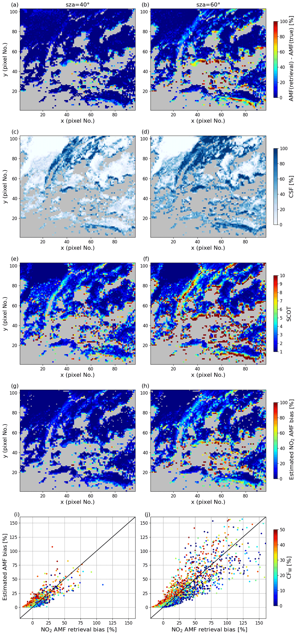
Figure 17Example of our parameterization approach for the NO2 retrieval bias in the cloud shadow for the LEO cases with surface albedo =0.05, VZA =0∘, and SZA =40∘ (a, c, e, g, i) and 60∘ (b, d, f, h, j). Panels (a) and (b) show the bias of NO2 retrieval based on the standard retrieval algorithm using O2–O2 cloud correction. Grey shaded pixels indicate cloudy pixels. Panels (c) and (d) are the cloud shadow fraction. Panels (e) and (f) are the averaged slant cloud optical thickness. Panels (g) and (h) are the estimated NO2 bias using the Eq. (9). Panels (i) and (j) compare the true retrieval bias with the estimation; only the pixels with the cloud shadow fraction >10 % and slant cloud optical thickness >1 are used in the analysis. The colours represent the cloud radiance fraction from the retrieval.
4.3 Comparison of mitigation strategies for observed data
In order to investigate the impact of mitigation strategies discussed above on observed data, one needs to identify 3D cloud cases. For TROPOMI, we selected two cases (24 March and 30 December 2019) as discussed in Kylling et al. (2022). The latter case is used to investigate the effect of the proposed mitigation strategies on real data. For this case, there is a clear cloud band and a completely cloud-free scene with a large extent of a cloud shadow region in the north of the cloud (as shown in Fig. 18). The first correction approach (Sect. 4.1.1) is not applied to the TROPOMI data, since cloud fractions from the current TROPOMI cloud retrievals are confined to the interval [0,1] (Loyola et al., 2018; van Geffen et al., 2022), and building a new extended TROPOMI cloud retrieval is beyond the scope of this study.
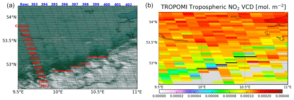
Figure 18Example of satellite observation for the cloud shadow band on 30 December 2019. (a) The VIIRS RGB image with TROPOMI footprint. (b) The TROPOMI tropospheric NO2 VCDs; the grey regions represent pixels with CFw>50 %. The red (left) and black (right) lines indicate the cloud edge in the along-track direction from row 393 to 398.
First, our NO2 AMF retrieval script is adapted to TROPOMI. The effective surface albedo is fitted at 437.5 nm, which is the wavelength used for the AMF calculation. The O2–O2 SCD retrieval follows Veefkind et al. (2016) and includes a correction for its dependency on the temperature profile (Veefkind et al., 2016). The NO2 retrieval using the standard approach, together with the two retrievals using our proposed correction methods (fitted surface albedo and O2–O2 SCD), is shown in Fig. 19a. The three retrievals agree very well over the clear-sky region (white region). In the cloud shadow, the NO2 VCD using the correction approaches is larger than the corresponding NO2 column from the standard retrieval. In order to validate the correction approaches, we compare the averaged NO2 column in the cloud shadow and around the shadow as shown in Fig. 19b. The NO2 around the shadow is the average of the NO2 column using the standard approach for 4 pixels in the clear region and 4 pixels in the cloudy region. We assume that this represents the true NO2 column. The standard NO2 column in the cloud shadow is systematically lower than around the cloud shadow region due to the 3D cloud effects, and the differences are reduced when the retrieval includes the correction in the shadow. The AMF corrected by O2–O2 SCD improves the retrieval for all cases, while the AMF calculated by the effective surface albedo seems to overcorrect for rows 395 and 396. For these cases, the retrieved surface albedo for the pixels in the cloud shadow is 0 (lower limit), which is similar to the results that have been discussed in Sect. 4.1.2.

Figure 19Comparison of the NO2 VCDs using a standard retrieval algorithm and retrievals implementing the correction approaches discussed in Sect. 4.1.2 and 4.1.3. The data use TROPOMI measurements over the cloud shadow band for 30 December 2019. (a) The NO2 retrieval based on three approaches as a function of latitude for TROPOMI row 394. The dark grey, light grey, and white regions represent the cloudy, shadow, and clean regions, respectively. (b) Difference of the NO2 columns in the cloud shadow and that around shadow for the standard retrieval and the retrieval including a correction in the cloud shadow for row 393–398, and the average bias over all rows is given in the legend. See text for further details.
The parameterization approach relies on parameters, such as cloud shadow fraction, slant cloud optical thickness, the NO2 profile, and neighbouring cloud top height. In practice, the NO2 profile height is based on the NO2 vertical profiles from the TM5-MP model (van Geffen et al., 2022), which is used for the calculation of the AMF in the operational product. The cloud top height is a maximum of VIIRS cloud height for the neighbouring pixels of the TROPOMI pixel. The COT and cloud shadow mask are not available for VIIRS data for this case, probably due to the large SZA (≈80∘). Therefore we use an alternative approach based on the correlation of COT and CFr from the 1D simulations described in Sect. 2.5, taking advantage of the fact that the CFr depends strongly on the COT and much less on the surface albedo and the solar and viewing geometries. The SCOT is computed using the SZA of the selected TROPOMI pixel and an averaged COT calculated over 5 neighbouring TROPOMI pixels. Since the VIIRS CTH is up to 7 km, the cloud shadow area is about 40 km, which corresponds to 4.5 TROPOMI pixels. The cloud shadow fraction is based on the VIIRS M3 band. The averaged VIIRS reflectance over the clear pixel near the cloud edge is used as a reference to define whether the VIIRS pixels are in the cloud shadow, and then the cloud shadow fraction is computed. The averaged parameters over the shadow are shown in Fig. 20a.
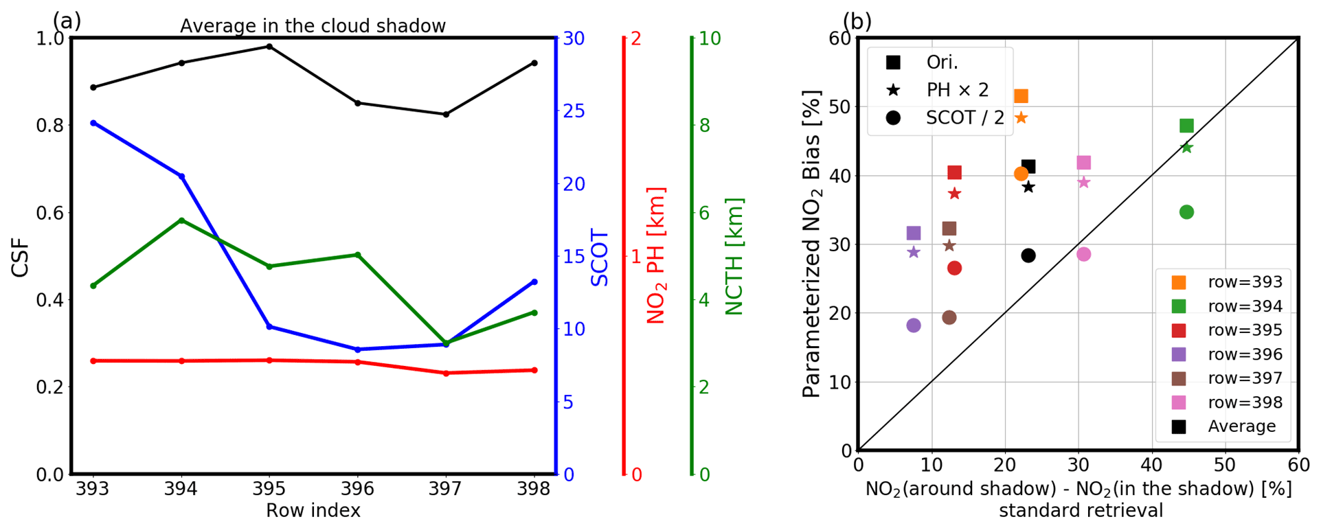
Figure 20Estimation of NO2 retrieval biases over the cloud shadow bands from TROPOMI measurements on 30 December 2019. (a) Averaged parameters in the cloud shadow, which are used to estimate the bias. (b) Comparison of the estimated bias and the NO2 bias calculated based on the difference of NO2 retrieval around and in the cloud shadow. The black is the average over all the rows, and the stars and the circles correspond to the estimation using doubled NO2 profile height and halved slant cloud optical thickness. See the text for further details.
Finally, we estimate the NO2 VCD bias using Eq. (9) for TROPOMI pixels located in the cloud shadow, weighted by the NO2 VCD from the standard retrieval. In Fig. 20b, the averaged NO2 bias from the parameterization approach in the cloud shadow is compared with the difference of the NO2 retrieval around and in the cloud shadow; each point represents the analysis for one row. Although there are only a few data points, the estimated bias shows a positive correlation with the NO2 bias by comparing NO2 retrieval in and around the shadow. The estimated value is however slightly larger. Besides the error due to the parameterization approach itself, the error from deriving various parameters from the satellite images may lead to uncertainties. Doubling the NO2 profile height or halving the slant cloud optical thickness led to a reduction of the bias by 3 % or 13 % respectively (see Fig. 20b). Although it is error-prone due to the complexity of the problem and the difficulty to extract relevant parameters from imager data, the parameterization approach might be very useful to identify satellite pixels likely affected by significant 3D clouds biases.
It should also be noted that other sources of uncertainty in the NO2 retrieval itself may affect such comparison results, in particular the uncertainty on parameters used in the AMF calculation, e.g. the a priori NO2 profile shape. For high SZAs, uncertainties due to the slant column retrieval from the spectral fit and the stratospheric correction are also important. In addition, the true NO2 column is unknown, and NO2 columns usually show a considerable spatial variability, especially over polluted regions. Therefore, without additional independent measurements, the 3D effects on NO2 retrievals are difficult to identify, and correction approaches are hard to validate.
In this study, we have investigated the impact of 3D clouds on the tropospheric NO2 retrieval from UV–visible sensors. In order to identify and quantify this impact, we first applied standard NO2 retrieval methods, including cloud corrections to synthetic data generated by the 3D Monte Carlo radiative transfer model MYSTIC. Since the cloud correction schemes are based on a simple cloud model, the accuracy of the NO2 retrieval depends on not only the cloud retrieval, but also on other factors, such as the NO2 profile. The analysis in the study focused mainly on the error of the NO2 retrieval due to the 3D cloud effects. Then, a sensitivity study for the simulations including a box cloud was made, and dependencies on various parameters were investigated. Finally, possible mitigation strategies such as AMF correction methods and a parameterization approach were investigated and compared based on realistic simulations with LES clouds and observed data.
The most significant biases are related to cloud shadow effects. The cloud products used in the NO2 retrieval treat the cloud shadow pixels as cloud-free, resulting in large positive biases (up to more than 100 %) in the NO2 AMF calculation. The magnitude of cloud shadow effects depends on the NO2 profile and is larger for polluted profiles, i.e. for profiles containing significant NO2 amounts in the lower troposphere. The retrieval bias depends strongly on the cloud shadow fraction, and we find that pixels affected by 3D cloud effects can be corrected using an independent pixel approximation, which assumes that the retrieval bias can be written as a linear combination of the bias from the clear, cloud shadow and cloudy parts. If the cloud shadow area is smaller than the size of the satellite pixel, the cloud shadow effect will be significantly reduced. We conclude that cloud shadow fraction, NO2 profile, cloud optical thickness, and solar zenith angle, as well as surface albedo are the most important parameters to characterize 3D cloud impacts on NO2 retrievals.
Several approaches to correct the NO2 retrieval in the cloud shadow were explored based on both synthetic and observational data. These include (a) the AMF retrieval using cloud correction based on the extended O2–O2/FRESCO and CAL cloud retrievals, (b) calculation of the AMF using an effective surface albedo based on the measured radiance, and (c) correction of the NO2 retrieval using the difference of retrieved O2–O2 SCDs and reference calculations for a clear scene under the same geometry. The latter two methods can partly correct the cloud shadow effects in the NO2 retrievals. However, they are limited to cloud-free conditions. Furthermore, an approach was developed to identify in real data the NO2 measurements that are likely biased due to 3D cloud effects. The approach estimates the size of the NO2 bias using an empirical formula based on relationships derived from an analysis of model simulations. It provides a way to improve the current data flagging method.
In future work, the development of improved parameterization approach accounting for 3D cloud effects requires an appropriate and extended synthetic dataset covering a large range of atmospheric situations. Since 3D cloud effects depend in a non-trivial way on many parameters, machine learning approaches may provide a fruitful way for development of parameterization mitigation methods of 3D cloud impacts on UV and visible trace gas products. Another possible mitigation method is to develop more sophisticated cloud retrievals, which account for the 3D effects, are feasible to apply to satellite observation, and can easily adapt to current trace gas retrieval algorithms.
Moreover, the validation of the mitigation methods is needed. Such validation is non-trivial and possibly requires new experimental approaches for measurements of both cloud shape and trace gas spatial variation. For example, for cloud shadow effect estimation, a cloud shadow product is needed. The 3D radiative transfer simulations as those utilized in this study, but for all relevant spectral bands, may be used to test and validate such algorithms. However, a complete validation must include comparison with independent measurements.
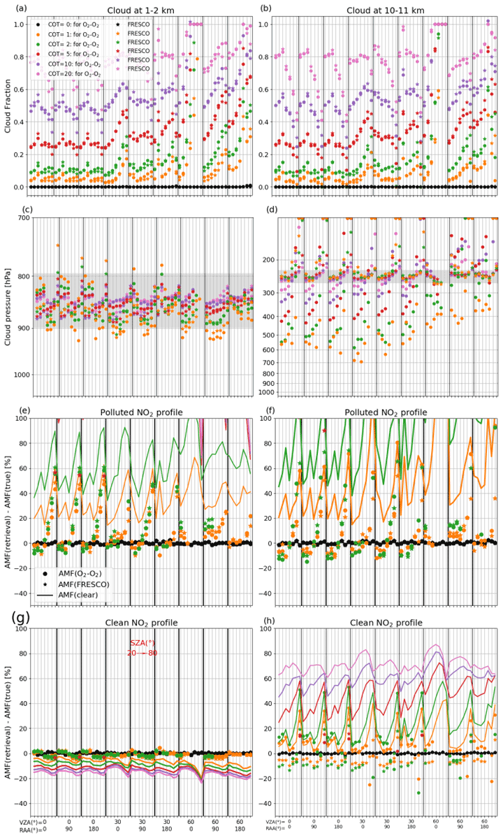
Figure A1Examples of cloud and NO2 retrieval for 1D cloud scenes, discussed in Sect. 2.5, with 1–2 km (a, c, e, g) and 10–11 km (b, d, f, h) cloud height. Panels (a) and (b) show O2–O2 and FRESCO cloud fraction retrievals, and panels (c) and (d) are the cloud pressure retrieval from O2–O2 and FRESCO cloud algorithms; the grey regions indicate the true cloud layer. Panels (e)–(h) compare the bias of the NO2 AMFs using cloud correction based on O2–O2 and FRESCO cloud products, as well as the AMFs without cloud correction, for polluted (e, f) and clean (g, h) conditions. The cloud correction is applied when the pixels with CFw are less than 50 %. The x axis represents the cases with different geometries. The variety of colours represents the cases with different cloud optical thicknesses.


The QDOAS software for DOAS retrieval of trace gases is available from https://uv-vis.aeronomie.be/software/QDOAS/ (last access: 24 September 2022; Danckaert et al., 2022). VIIRS data were accessed through the NOAA Comprehensive Large Array-Data Stewardship System (CLASS, https://www.bou.class.noaa.gov, last access: 24 September 2022; NOAA, 2022). TROPOMI data were downloaded from https://s5phub.copernicus.eu/ (last access: 24 September 2022; Copernicus Open Access Hub, 2022).
HY is the main contributor to the study. He applied the NO2 retrieval algorithm on the synthetic data, analysed the impact of 3D cloud on the retrieval, investigated the possible mitigation strategies, and led the writing of this paper. CE provided synthetic data from 3D radiative transfer simulations. AK contributed to data analysis and software development. MVR, KS, BV, and BM contributed to conceptualization and methodology. All co-authors were involved in the discussion of results and the writing of this article.
At least one of the (co-)authors is a member of the editorial board of Atmospheric Measurement Techniques. The peer-review process was guided by an independent editor, and the authors also have no other competing interests to declare.
Publisher’s note: Copernicus Publications remains neutral with regard to jurisdictional claims in published maps and institutional affiliations.
We would like to thank the two anonymous referees for their comments.
This research has been supported by the European Space Agency (3DCATS project no. 4000124890/18/NL/FF/gp).
This paper was edited by Diego Loyola and reviewed by two anonymous referees.
Acarreta, J. R., De Haan, J. F., and Stammes, P.: Cloud pressure retrieval using the O2-O2 absorption band at 477 nm, J. Geophys. Res.-Atmos., 109, D05204, https://doi.org/10.1029/2003JD003915, 2004. a, b, c
Anderson, G., Clough, S., Kneizys, F., Chetwynd, J., and Shettle, E.: AFGL atmospheric constituent profiles (0–120km), in: Environmental research papers, Hanscom AFB, Mass., no. 954, AFGL-TR, 86-0110, Optical Physics Division, Air Force Geophysics Laboratory, U.S. Air Force Geophysics Laboratory, Optical Physics Division, Hanscom AFB edn., 1986. a, b
Bodhaine, B. A., Wood, N. B., Dutton, E. G., and Slusser, J. R.: On Rayleigh optical depth calculations, J. Atmos. Ocean Tech., 16, 1854–1861, 1999. a
Boersma, K. F., Eskes, H. J., and Brinksma, E. J.: Error analysis for tropospheric NO2 retrieval from space, J. Geophys. Res., 109, D04311, https://doi.org/10.1029/2003JD003962, 2004. a, b, c, d, e
Boersma, K. F., Eskes, H. J., Veefkind, J. P., Brinksma, E. J., van der A, R. J., Sneep, M., van den Oord, G. H. J., Levelt, P. F., Stammes, P., Gleason, J. F., and Bucsela, E. J.: Near-real time retrieval of tropospheric NO2 from OMI, Atmos. Chem. Phys., 7, 2103–2118, https://doi.org/10.5194/acp-7-2103-2007, 2007. a
Boersma, K. F., Eskes, H. J., Dirksen, R. J., van der A, R. J., Veefkind, J. P., Stammes, P., Huijnen, V., Kleipool, Q. L., Sneep, M., Claas, J., Leitão, J., Richter, A., Zhou, Y., and Brunner, D.: An improved tropospheric NO2 column retrieval algorithm for the Ozone Monitoring Instrument, Atmos. Meas. Tech., 4, 1905–1928, https://doi.org/10.5194/amt-4-1905-2011, 2011. a, b
Boersma, K. F., Eskes, H. J., Richter, A., De Smedt, I., Lorente, A., Beirle, S., van Geffen, J. H. G. M., Zara, M., Peters, E., Van Roozendael, M., Wagner, T., Maasakkers, J. D., van der A, R. J., Nightingale, J., De Rudder, A., Irie, H., Pinardi, G., Lambert, J.-C., and Compernolle, S. C.: Improving algorithms and uncertainty estimates for satellite NO2 retrievals: results from the quality assurance for the essential climate variables (QA4ECV) project, Atmos. Meas. Tech., 11, 6651–6678, https://doi.org/10.5194/amt-11-6651-2018, 2018. a, b
Bucsela, E. J., Celarier, E. A., Wenig, M. O., Gleason, J. F., Veefkind, J. P., Boersma, K. F., and Brinksma, E. J.: Algorithm for NO2 vertical column retrieval from the ozone monitoring instrument, IEEE T. Geosci. Remote, 44, 1245–1258, https://doi.org/10.1109/TGRS.2005.863715, 2006. a
Bucsela, E. J., Krotkov, N. A., Celarier, E. A., Lamsal, L. N., Swartz, W. H., Bhartia, P. K., Boersma, K. F., Veefkind, J. P., Gleason, J. F., and Pickering, K. E.: A new stratospheric and tropospheric NO2 retrieval algorithm for nadir-viewing satellite instruments: applications to OMI, Atmos. Meas. Tech., 6, 2607–2626, https://doi.org/10.5194/amt-6-2607-2013, 2013. a
Copernicus Open Access Hub: S5P, ESA [data set], https://s5phub.copernicus.eu/, last access: 24 September 2022. a
Danckaert, T., Fayt, C., Van Roozendael, M., De Smedt, I., Letocart, V., Merlaud, A., and Pinardi, G.: QDOAS, Royal Belgian Institute for Space Aeronomy [code], https://uv-vis.aeronomie.be/software/QDOAS/, last access: 24 September 2022. a
De Smedt, I., Theys, N., Yu, H., Danckaert, T., Lerot, C., Compernolle, S., Van Roozendael, M., Richter, A., Hilboll, A., Peters, E., Pedergnana, M., Loyola, D., Beirle, S., Wagner, T., Eskes, H., van Geffen, J., Boersma, K. F., and Veefkind, P.: Algorithm theoretical baseline for formaldehyde retrievals from S5P TROPOMI and from the QA4ECV project, Atmos. Meas. Tech., 11, 2395–2426, https://doi.org/10.5194/amt-11-2395-2018, 2018. a, b
De Smedt, I., Pinardi, G., Vigouroux, C., Compernolle, S., Bais, A., Benavent, N., Boersma, F., Chan, K.-L., Donner, S., Eichmann, K.-U., Hedelt, P., Hendrick, F., Irie, H., Kumar, V., Lambert, J.-C., Langerock, B., Lerot, C., Liu, C., Loyola, D., Piters, A., Richter, A., Rivera Cárdenas, C., Romahn, F., Ryan, R. G., Sinha, V., Theys, N., Vlietinck, J., Wagner, T., Wang, T., Yu, H., and Van Roozendael, M.: Comparative assessment of TROPOMI and OMI formaldehyde observations and validation against MAX-DOAS network column measurements, Atmos. Chem. Phys., 21, 12561–12593, https://doi.org/10.5194/acp-21-12561-2021, 2021. a
Dipankar, A., Stevens, B., Heinze, R., Moseley, C., Zängl, G., Giorgetta, M. A., and Brdar, S.: Large eddy simulation using the general circulation model ICON, J. Adv. Model. Earth Sy., 7, 963–986, https://doi.org/10.1002/2015MS000431, 2015. a
Emde, C., Buras, R., and Mayer, B.: ALIS: An efficient method to compute high spectral resolution polarized solar radiances using the Monte Carlo approach, J. Quant. Spectrosc. Ra., 112, 1622–1631, 2011. a
Emde, C., Buras-Schnell, R., Kylling, A., Mayer, B., Gasteiger, J., Hamann, U., Kylling, J., Richter, B., Pause, C., Dowling, T., and Bugliaro, L.: The libRadtran software package for radiative transfer calculations (version 2.0.1), Geosci. Model Dev., 9, 1647–1672, https://doi.org/10.5194/gmd-9-1647-2016, 2016. a
Emde, C., Yu, H., Kylling, A., van Roozendael, M., Stebel, K., Veihelmann, B., and Mayer, B.: Impact of 3D cloud structures on the atmospheric trace gas products from UV–Vis sounders – Part 1: Synthetic dataset for validation of trace gas retrieval algorithms, Atmos. Meas. Tech., 15, 1587–1608, https://doi.org/10.5194/amt-15-1587-2022, 2022. a, b, c, d, e, f, g
Eriksson, P., Buehler, S. A., Davis, C. P., Emde, C., and Lemke, O.: ARTS, the atmospheric radiative transfer simulator, version 2, J. Quant. Spectrosc. Ra., 112, 1551–1558, 2011. a
Koelemeijer, R. B. A., Stammes, P., Hovenier, J. W., and de Haan, J. F.: A fast method for retrieval of cloud parameters using oxygen A band measurements from the Global Ozone Monitoring Experiment, J. Geophys. Res., 106, 3475–3490, 2001. a, b
Krijger, J. M., van Weele, M., Aben, I., and Frey, R.: Technical Note: The effect of sensor resolution on the number of cloud-free observations from space, Atmos. Chem. Phys., 7, 2881–2891, https://doi.org/10.5194/acp-7-2881-2007, 2007. a
Kylling, A., Emde, C., Yu, H., van Roozendael, M., Stebel, K., Veihelmann, B., and Mayer, B.: Impact of 3D cloud structures on the atmospheric trace gas products from UV–Vis sounders – Part 3: Bias estimate using synthetic and observational data, Atmos. Meas. Tech., 15, 3481–3495, https://doi.org/10.5194/amt-15-3481-2022, 2022. a, b, c
Lerot, C., Stavrakou, T., De Smedt, I., Müller, J.-F., and Van Roozendael, M.: Glyoxal vertical columns from GOME-2 backscattered light measurements and comparisons with a global model, Atmos. Chem. Phys., 10, 12059–12072, https://doi.org/10.5194/acp-10-12059-2010, 2010. a
Levelt, P., Veefkind, J., Kerridge, B., Siddans, R., de Leeuw, G., Remedios, J., and Coheur, P.: Observation Techniques and Mission Concepts for Atmospheric Chemistry (CAMELOT), Tech. rep., Report RP-CAM-KNMI-050, KNMI, European Space Agency, Noordwijk, the Netherlands, 2009. a
Liu, S., Valks, P., Pinardi, G., De Smedt, I., Yu, H., Beirle, S., and Richter, A.: An improved total and tropospheric NO2 column retrieval for GOME-2, Atmos. Meas. Tech., 12, 1029–1057, https://doi.org/10.5194/amt-12-1029-2019, 2019. a
Liu, S., Valks, P., Pinardi, G., Xu, J., Argyrouli, A., Lutz, R., Tilstra, L. G., Huijnen, V., Hendrick, F., and Van Roozendael, M.: An improved air mass factor calculation for nitrogen dioxide measurements from the Global Ozone Monitoring Experiment-2 (GOME-2), Atmos. Meas. Tech., 13, 755–787, https://doi.org/10.5194/amt-13-755-2020, 2020. a, b, c, d
Liu, S., Valks, P., Pinardi, G., Xu, J., Chan, K. L., Argyrouli, A., Lutz, R., Beirle, S., Khorsandi, E., Baier, F., Huijnen, V., Bais, A., Donner, S., Dörner, S., Gratsea, M., Hendrick, F., Karagkiozidis, D., Lange, K., Piters, A. J. M., Remmers, J., Richter, A., Van Roozendael, M., Wagner, T., Wenig, M., and Loyola, D. G.: An improved TROPOMI tropospheric NO2 research product over Europe, Atmos. Meas. Tech., 14, 7297–7327, https://doi.org/10.5194/amt-14-7297-2021, 2021. a, b
Lorente, A., Folkert Boersma, K., Yu, H., Dörner, S., Hilboll, A., Richter, A., Liu, M., Lamsal, L. N., Barkley, M., De Smedt, I., Van Roozendael, M., Wang, Y., Wagner, T., Beirle, S., Lin, J.-T., Krotkov, N., Stammes, P., Wang, P., Eskes, H. J., and Krol, M.: Structural uncertainty in air mass factor calculation for NO2 and HCHO satellite retrievals, Atmos. Meas. Tech., 10, 759–782, https://doi.org/10.5194/amt-10-759-2017, 2017. a, b
Loyola, D. G., Thomas, W., Livschitz, Y., Ruppert, T., Albert, P., and Hollmann, R.: Cloud properties derived from GOME/ERS-2 backscatter data for trace gas retrieval, IEEE T. Geosci. Remote, 45, 2747–2758, https://doi.org/10.1109/TGRS.2007.901043, 2007. a
Loyola, D. G., Gimeno García, S., Lutz, R., Argyrouli, A., Romahn, F., Spurr, R. J. D., Pedergnana, M., Doicu, A., Molina García, V., and Schüssler, O.: The operational cloud retrieval algorithms from TROPOMI on board Sentinel-5 Precursor, Atmos. Meas. Tech., 11, 409–427, https://doi.org/10.5194/amt-11-409-2018, 2018. a, b, c, d
Massie, S. T., Schmidt, K. S., Eldering, A., and Crisp, D.: Observational evidence of 3-D cloud effects in OCO-2 CO2 retrievals, J. Geophys. Res.-Atmos., 122, 7064–7085, https://doi.org/10.1002/2016JD026111, 2017. a
Massie, S. T., Cronk, H., Merrelli, A., O'Dell, C., Schmidt, K. S., Chen, H., and Baker, D.: Analysis of 3D cloud effects in OCO-2 XCO2 retrievals, Atmos. Meas. Tech., 14, 1475–1499, https://doi.org/10.5194/amt-14-1475-2021, 2021. a
Mayer, B.: Radiative transfer in the cloudy atmosphere, EPJ Web. Conf., 1, 75–99, 2009. a
Mayer, B. and Kylling, A.: Technical note: The libRadtran software package for radiative transfer calculations – description and examples of use, Atmos. Chem. Phys., 5, 1855–1877, https://doi.org/10.5194/acp-5-1855-2005, 2005. a
Nikolaeva, O. V., Bass, L. P., Germogenova, T. A., Kokhanovsky, A. A., Kuznetsov, V. S., and Mayer, B.: The influence of neighbouring clouds on the clear sky reflectance studied with the 3-D transport code RADUGA, J. Quant. Spectrosc. Ra., 94, 405–424, https://doi.org/10.1016/j.jqsrt.2004.09.037, 2005. a
NOAA: Comprehensive Large Array-data Stewardship System (CLASS), NOAA [data set], https://www.avl.class.noaa.gov, last access: 24 September 2022. a
Palmer, P. I., Jacob, D. J., Chance, K., Martin, R. V., Spurr, R. J., Kurosu, T. P., Bey, I., Yantosca, R., Fiore, A., and Li, Q.: Air mass factor formulation for spectroscopic measurements from satellites: Application to formaldehyde retrievals from the Global Ozone Monitoring Experiment, J. Geophys. Res.-Atmos., 106, 14539–14550, https://doi.org/10.1029/2000JD900772, 2001. a
Platt, U. and Stutz, J.: Differential Optical Absorption Spectroscopy: Principles and Applications, Springer-Verlag Berlin Heidelberg, https://doi.org/10.1007/978-3-540-75776-4, 2008. a
Rothman, L. S., Gordon, I. E., Babikov, Y., Barbe, A., Chris Benner, D., Bernath, P. F., Birk, M., Bizzocchi, L., Boudon, V., Brown, L. R., Campargue, A., Chance, K., Cohen, E. A., Coudert, L. H., Devi, V. M., Drouin, B. J., Fayt, A., Flaud, J. M., Gamache, R. R., Harrison, J. J., Hartmann, J. M., Hill, C., Hodges, J. T., Jacquemart, D., Jolly, A., Lamouroux, J., Le Roy, R. J., Li, G., Long, D. A., Lyulin, O. M., Mackie, C. J., Massie, S. T., Mikhailenko, S., Müller, H. S., Naumenko, O. V., Nikitin, A. V., Orphal, J., Perevalov, V., Perrin, A., Polovtseva, E. R., Richard, C., Smith, M. A., Starikova, E., Sung, K., Tashkun, S., Tennyson, J., Toon, G. C., Tyuterev, V. G., and Wagner, G.: The HITRAN2012 molecular spectroscopic database, J. Quant. Spectrosc. Ra., 130, 4–50, https://doi.org/10.1016/j.jqsrt.2013.07.002, 2013. a
Schwaerzel, M., Emde, C., Brunner, D., Morales, R., Wagner, T., Berne, A., Buchmann, B., and Kuhlmann, G.: Three-dimensional radiative transfer effects on airborne and ground-based trace gas remote sensing, Atmos. Meas. Tech., 13, 4277–4293, https://doi.org/10.5194/amt-13-4277-2020, 2020. a
Schwaerzel, M., Brunner, D., Jakub, F., Emde, C., Buchmann, B., Berne, A., and Kuhlmann, G.: Impact of 3D radiative transfer on airborne NO2 imaging remote sensing over cities with buildings, Atmos. Meas. Tech., 14, 6469–6482, https://doi.org/10.5194/amt-14-6469-2021, 2021. a
Sneep, M., de Haan, J. F., Stammes, P., Wang, P., Vanbauce, C., Joiner, J., Vasilikov, A. P., and Levelt, P. F.: Three-way comparison between OMI and PARASOL cloud pressure products, J. Geophys. Res., 113, D15S23, https://doi.org/10.1029/2007JD008694, 2008. a
Spurr, R. and Christi, M.: On the generation of atmospheric property Jacobians from the (V)LIDORT linearized radiative transfer models, J. Quant. Spectrosc. Ra., 142, 109–115, https://doi.org/10.1016/j.jqsrt.2014.03.011, 2014. a
Spurr, R. and Christi, M.: The LIDORT and VLIDORT Linearized Scalar and Vector Discrete Ordinate Radiative Transfer Models: Updates in the Last 10 Years, Springer, Cham, https://doi.org/10.1007/978-3-030-03445-0_1, 2019. a
Spurr, R., Kurosu, T. P., and Chance, K. V.: A linearized discrete ordinate radiative transfer model for atmospheric remote-sensing retrieval, J. Quant. Spectrosc. Ra., 68, 689–735, 2001. a
Stammes, P., Sneep, M., de Haan, J. F., Veefkind, J. P., Wang, P., and Levelt, P. F.: Effective cloud fractions from the Ozone Monitoring Instrument: Theoretical framework and validation, J. Geophys. Res., 113, D16S38, https://doi.org/10.1029/2007JD008820, 2008. a, b
Theys, N., De Smedt, I., Van Gent, J., Danckaert, T., Wang, T., Hendrick, F., Stavrakou, T., Bauduin, S., Clarisse, L., Li, C., Krotkov, N., Yu, H., Brenot, H., and Van Roozendael, M.: Sulfur dioxide vertical column DOAS retrievals from the Ozone Monitoring Instrument: Global observations and comparison to ground-based and satellite data, J. Geophys. Res.-Atmos., 120, 2470–2491, https://doi.org/10.1002/2014JD022657, 2015. a
Theys, N., De Smedt, I., Yu, H., Danckaert, T., van Gent, J., Hörmann, C., Wagner, T., Hedelt, P., Bauer, H., Romahn, F., Pedergnana, M., Loyola, D., and Van Roozendael, M.: Sulfur dioxide retrievals from TROPOMI onboard Sentinel-5 Precursor: algorithm theoretical basis, Atmos. Meas. Tech., 10, 119–153, https://doi.org/10.5194/amt-10-119-2017, 2017. a, b
Valks, P., Pinardi, G., Richter, A., Lambert, J.-C., Hao, N., Loyola, D., Van Roozendael, M., and Emmadi, S.: Operational total and tropospheric NO2 column retrieval for GOME-2, Atmos. Meas. Tech., 4, 1491–1514, https://doi.org/10.5194/amt-4-1491-2011, 2011. a
van Geffen, J., Boersma, K. F., Eskes, H., Sneep, M., ter Linden, M., Zara, M., and Veefkind, J. P.: S5P TROPOMI NO2 slant column retrieval: method, stability, uncertainties and comparisons with OMI, Atmos. Meas. Tech., 13, 1315–1335, https://doi.org/10.5194/amt-13-1315-2020, 2020. a
van Geffen, J. H. G. M., Eskes, H. J., Boersma, K. F., Maasakkers, J. D., and Veefkind, J. P.: TROPOMI ATBD of the total and tropospheric NO2 data products, Tech. rep., Report S5P-KNMI-L2-0005-RP, version 2.4.0, KNMI, De Bilt, the Netherlands, https://sentinel.esa.int/web/sentinel/technical-guides/sentinel-5p/products-algorithms/, last access: 6 October 2022. a, b, c
Várnai, T. and Marshak, A.: MODIS observations of enhanced clear sky reflectance near clouds, Geophys. Res. Lett., 36, L06807, https://doi.org/10.1029/2008GL037089, 2009. a
Várnai, T., Marshak, A., and Yang, W.: Multi-satellite aerosol observations in the vicinity of clouds, Atmos. Chem. Phys., 13, 3899–3908, https://doi.org/10.5194/acp-13-3899-2013, 2013. a
Veefkind, J. P., de Haan, J. F., Sneep, M., and Levelt, P. F.: Improvements to the OMI O2–O2 operational cloud algorithm and comparisons with ground-based radar–lidar observations, Atmos. Meas. Tech., 9, 6035–6049, https://doi.org/10.5194/amt-9-6035-2016, 2016. a, b, c, d
Wang, P., Stammes, P., van der A, R., Pinardi, G., and van Roozendael, M.: FRESCO+: an improved O2 A-band cloud retrieval algorithm for tropospheric trace gas retrievals, Atmos. Chem. Phys., 8, 6565–6576, https://doi.org/10.5194/acp-8-6565-2008, 2008. a, b, c
Zängl, G., Reinert, D., Rípodas, P., and Baldauf, M.: The ICON (ICOsahedral Non-hydrostatic) modelling framework of DWD and MPI-M: Description of the non-hydrostatic dynamical core, Q. J. Roy. Meteor. Soc., 141, 563–579, https://doi.org/10.1002/qj.2378, 2015. a