the Creative Commons Attribution 4.0 License.
the Creative Commons Attribution 4.0 License.
 | 14 Oct 2022
3D trajectories and velocities of rainfall drops in a multifractal turbulent wind field
Ioulia Tchiguirinskaia
Daniel Schertzer
Weather radars measure rainfall in altitude, whereas hydro-meteorologists are mainly interested in rainfall at ground level. During their fall, drops are advected by the wind, which affects the location of the measured field.
The governing equation of a rain drop's motion relates the acceleration to the forces of gravity and buoyancy along with the drag force. It depends non-linearly on the instantaneous relative velocity between the drop and the local wind, which yields complex behaviour. Here, the drag force is expressed in a standard way with the help of a drag coefficient expressed as a function of the Reynolds number. Corrections accounting for the oblateness of drops greater than 1–2 mm are suggested and validated through a comparison of the retrieved “terminal fall velocity” (i.e. without wind) with commonly used relationships in the literature.
An explicit numerical scheme is then implemented to solve this equation for a 3+1D turbulent wind field, and hence analyse the temporal evolution of the velocities and trajectories of rain drops during their fall. It appears that multifractal features of the input wind are simply transferred to the drop velocity with an additional fractional integration whose level depends on the drop size, and a slight time shift. Using an actual high-resolution 3D sonic anemometer and a scale invariant approach to simulate realistic fluctuations of wind in space, trajectories of drops of various sizes falling form 1500 m are studied. For a strong wind event, drops located within a radar gate in altitude during 5 min are spread on the ground over an area of the size of a few kilometres. The spread for drops of a given diameter is found to cover a few radar pixels. Consequences on measurements of hydro-meteorological extremes that are needed to improve the resilience of urban areas are discussed.
- Article
(3661 KB) - Full-text XML
- BibTeX
- EndNote


During their fall, drops are advected by wind. Quantitative rainfall estimation with the help of weather radars is affected by this issue since drops can be displaced horizontally between their measurement location in altitude and their ground impact location, which is of interest for hydro-meteorologists. This effect is usually called wind drift in the literature and sometimes wind advection. The potential bias and uncertainty introduced in radar measurements is stronger at higher resolution, i.e. typically with pixel sizes smaller than 1–2 km2, which are needed for urban applications, for example. Collier (1999) suggests that correction schemes should be implemented for this kind or higher radar resolution. Lauri et al. (2012) reported that far from the radar (i.e. typically more than 150 km), even with low elevation (0.3∘), displacements of few tens of kilometres are found, which actually distort the measured area.
Most correction schemes rely on the use of 4D wind profiles derived from numerical prediction models (Mittermaier et al., 2004; Lack and Fox, 2007; Lauri et al., 2012; Sandford, 2015) or a combination of them with reanalysis (Dai et al., 2013, 2019; Yang et al., 2020). The latter also accounts for drop size distribution (DSD). They report an improvement by ≈3 % of the correlation between radar and rain gauge measurement and a reduction of discrepancy of ≈18 % over eight selected events. Lack and Fox (2007) directly used Doppler radar wind measurement at 2.5 km scale to adjust for the wind drift effect. In general, correction schemes use wind data of rather coarse resolution (typically km(s)) and assume a constant wind shear. Nevertheless, some variability at smaller space-time scales is usually acknowledged, especially during convective events, i.e. those for which wind drift causes the greatest uncertainty (Lack and Fox, 2007).
Wind effects on rainfall drops is also reported to generate discrepancies between the vertical velocities measured and expected terminal fall velocities. For example, Montero-Martínez and García-García (2016) studied events with calm, light and moderate wind with various rainfall levels and found a widening of the fall velocity distribution under windy conditions. They found super-terminal drops only for diameters <0.7 mm and more often under wind conditions. Sub-terminal fall velocities for drops of sizes up to 2 mm are reported. Bringi et al. (2018) found that under low wind speed and turbulence, no discrepancies with expectations are found, while under high wind speed and turbulence, there is a clear widening of the distribution. A linear decrease of the mean fall velocity with increasing turbulence intensity is reported. Maximum decreases of 25 %–30 % are observed. Thurai et al. (2019) also found such decreases for drops greater than 2 mm in high turbulence intensity conditions. It is associated to an asymmetry that also appears in the drop shape. They also found that horizontal drop velocities in both direction and magnitude show a “remarkable agreement” with the wind sensor at 10 m. Stout et al. (1995) explored the effect of the nonlinear drag coefficient on the fall velocity through numerical simulations. They showed that even heavy drops exhibited a reduced settling velocity in isotropic turbulence.
Turbulence is found to have contradictory effects on the distribution of the fall velocity. Indeed, increasing the turbulence level in windy and rainfall conditions will yield more collision and breakup, resulting in smaller drops inheriting the speed of larger parent drops, and hence observations of super-terminal velocities. On the other hand, turbulence is said to yield a decrease in fall velocities because drops (especially ones of <1 mm) are more affected by eddies.
Such findings on the discrepancies between observed and expected fall velocities have effects on the relation between rainfall and kinetic energy, i.e. the erosivity “power” of rainfall (Pedersen and Hasholt, 1995) and also building performance to outdoor conditions (Tian et al., 2018; Blocken et al., 2011).
The studies previously mentioned basically do not account for small-scale wind fluctuations in both space and time. In this paper, we suggest studying the behaviour of individual rainfall drops of various sizes in a high-resolution turbulent wind field. The variability of the wind is accounted for through the framework of universal multifractals (UM) (see Schertzer and Tchiguirinskaia, 2020, for a recent review). Such a physically based framework is designed to analyse and simulate geophysical fields exhibiting extreme variability over a wide range of space-time scales as wind. Drop oblateness is also accounted for.
The paper is organised as follows. In Sect. 2, a deterministic equation for the fall of individual oblate drops in a 3D field is derived and validated through the comparison of the terminal fall velocity obtained with commonly used formulas. In Sect. 3, the framework of universal multifractals is described briefly. Then, the drops are subjected to simulated multifractal fields as the wind input and multifractal behaviour of the horizontal drop velocity is assessed. Finally, in Sect. 4, 3D wind is reconstructed from high-resolution 3D sonic anemometer data and strong scaling assumptions. This field is used to study the trajectories of drops between falling from 1500 m to the ground.
2.1 Formulation of the equation
Let us denote the horizontal, lateral and vertical coordinates in a standard Cartesian framework with unit vectors (, , ). We aim at writing the motion equation of a particle of water (a drop) of velocity , density ρp and falling in the atmosphere under the influence of the gravity (where g=9.81 m s−2) and the wind (with three components). The density of the atmosphere is denoted ρair. The water particle is characterised by its equivolumic diameter Deq, which corresponds to the diameter of the sphere having the same total volume. Hence we have Vol . Finally, the relative velocity between the wind and the falling particle is ( is the vector with three components, while vrel is its Euclidean norm).
The drop is subjected to three forces:
-
The gravity equal to .
-
The buoyancy equal to .
-
The drag, which is commonly written as . Re is the common Reynolds number , where μair is the absolute viscosity of air; cD is the drag coefficient and depends in general on Re and Deq. The next section is devoted to its determination.
As a consequence, the equation of motion of the falling particle is given by Newton's second law, which equals the mass times the acceleration to the net force (here, it was divided by the mass):
2.2 Determination of the drag coefficient
Before discussing how the drag coefficient is determined, it should be recalled that the rainfall drops considered in this paper are not spherical. Indeed, drops greater than typically 1.5 mm become oblate in their fall. This oblateness increases with size. A very commonly used model consists in an ellipsoid with an axis ratio varying depending on the size. Thurai et al. (2007) showed that such model is too simplistic since drops are not symmetric in the direction perpendicular to their fall. Following an in-depth analysis of the drop shape assessed with the help of a 2D-video disdrometer (Kruger and Krajewski, 2002) in the measurement campaign of an artificial rainfall experiment, they suggested the following formula for the shape:
with:
This shape corresponding to a solid of revolution around the z axis is used in this paper. It is displayed in Fig. 2a for drops with equivolumic diameter ranging from 1.5 to 5.5 mm. It should be mentioned that computing the volume as an integral of the shape (Vol , see Fig. 1) yields minor differences with the expected volume of . They are highlighted in Fig. 2b. In order to account for this small difference, once an equivolumic diameter is set, the corresponding one that would lead to the expected volume from Eqs. (2) and (3) is computed from a correspondence table. The relationship, which is obviously close to the bisector, is displayed in Fig. 2c with the horizontal axis corresponding to the real Deq of the drop and the vertical axis to the Deq to be input in Eqs. (2) and (3) to retrieve the correct expected volume. A consequence is that the oblateness of drops will be considered only from an equivolumic diameter greater than 1.527 mm.
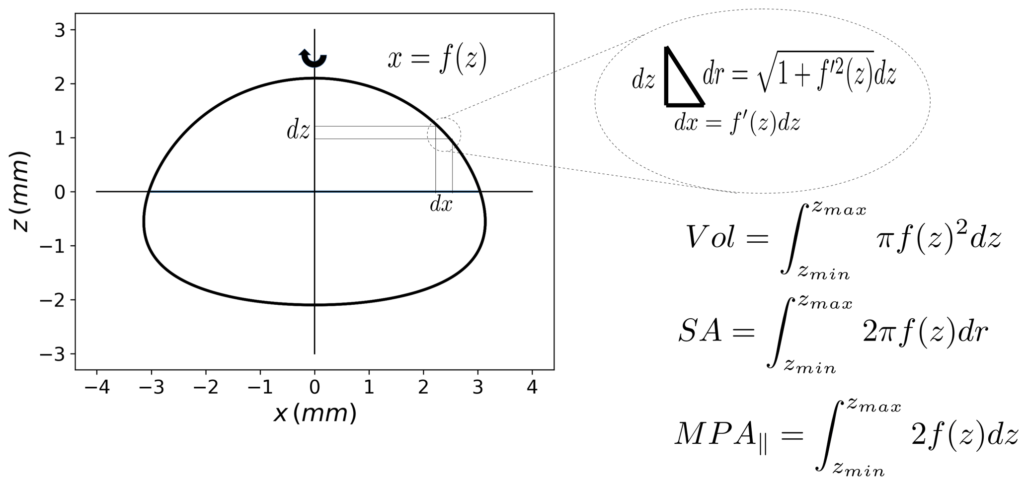
Figure 1Illustration of how the volume (Vol), the surface area (SA) and the mean projected longitudinal cross-sectional area (MPA∥) of the particle used in this paper can be computed via integral calculus. The drop is actually a solid of revolution around the “z” axis.
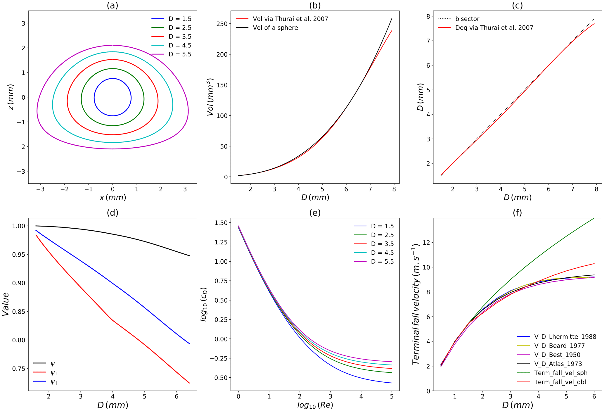
Figure 2(a) Drop shape model used in this paper; (b) drop volume vs. equivolumic diameter; (c) diameter relation to retrieved wanted volume; (d) parameters characterising non-spherical shape of drops vs. equivolumic diameter; (e) drag coefficient cD vs. Re number and (f) terminal fall velocity vs. equivolumic diameter.
For non-spherical shapes, it is quite tricky to compute the corresponding drag coefficient as a function of the Reynolds number. The literature about this issue is quite abundant, and the interested reader is referred to Chap. 4 of the PhD dissertation of Bagheri (2015) or Hölzer and Sommerfeld (2008) for details. In the approach that they implemented, three parameters are used to characterize the non-spherical shapes of the falling particle with the help of three dimensionless parameters: the sphericity, the crosswise sphericity and the lengthwise sphericity. The latter two depend on the orientation of the particle with regards to the flow. Here, it is assumed that drops are oriented perpendicularly to the flow, i.e. the “z” axis of Eq. (2) is parallel to . In the general case, these parameters may be complex to assess but with the shape derived from Eq. (2) (Thurai et al., 2007), theoretical formula can be obtained. See Fig. 1 for an illustration of the computations via integral calculus. The three parameters are:
-
The sphericity ψ, which is equal to ratio between the surface area (SA) of the equivolumic sphere to the actual surface area of the particle. It is equal to 1 for sphere and decreases for increasingly and fewer spherical particles; . That is, within the framework of this paper, we have SA .
-
The crosswise sphericity ψ⟂, which is equal to the ratio between the projected area of the volume equivalent sphere and the projected area of the particle normal to the falling direction (here, ); . It is equal to 1 for sphere and decreases for larger drops since they become oblate.
-
The lengthwise sphericity ψ∥, which is defined as the cross-sectional area of the volume equivalent sphere divided by the difference between half the surface area and the mean projected longitudinal cross-sectional area of particle (MPA ∥); . In the specific drop model of this paper, we have MPA (it basically corresponds to the 2D area of the drop plotted in Fig. 1).
The evolution of these parameters as a function of Deq for the drops considered is shown in Fig. 2d. The increasing oblateness of drops with increasing size is translated through the fact that the parameters are getting further away from 1. In order to define the drag coefficient, the corrections suggested by Hölzer and Sommerfeld (2008) to account for non-sphericity of particles are then implemented in the formula of White (1974), previously used by Stout et al. (1995) who worked only on spherical drops. This yields
The evolution of cD as a function of Re for various drop parameters is displayed in Fig. 2e and follows standard patterns.
2.3 Validation of the formula
In order to validate the developed equation, the retrieved terminal fall velocity is assessed for each equivolumic diameter. It corresponds to the velocity of the permanent regime with no wind, i.e. the drag plus the buoyancy exactly compensate the gravity. Computations are carried out with ρair=1.205 kg m−3, kg m−1 m−2, ρwater=998.2 kg m−3 g=9.81 m s−2, as in Stout et al. (1995).
The relation between the terminal fall velocity obtained vs. the equivolumic diameter is displayed in red in Fig. 2f. The developed equations enable us to retrieve the commonly used relation (Beard, 1977; Lhermitte, 1988; Best, 1950; Atlas et al., 1973) for drops of diameters of up to 4 mm. The deviations found when considering spherical drops (in green) are visible for diameters greater than 2 mm, which highlights the need to account for drop oblateness.
2.4 Numerical scheme for solving the equation
Equation (1) is solved numerically through the implementation of a simple Eulerian numerical scheme. Within such a framework: (i) a discretization of time with time step Δt is introduced yielding discrete time steps , where n is an integer; (ii) we aim at finding an approximation of at time step n denoted ; (iii) the first derivative in Eq. (1) is approximated as . This leads to the following equation for the numerical scheme:
where and cD,n are computed at time step tn using the formulas discussed in Sects. 2.1 and 2.2. Assuming some initial conditions (always no horizontal velocity and a vertical one equal to the terminal fall for the corresponding diameter), it is then possible to reconstruct the time series of velocity for the drops. From this, the temporal evolution of the position (i.e. the trajectory) is derived. It is necessary to properly assess the wind accounting for the current position of the drop. A time step of Δt=0.01 s is used in this paper, and it was checked that it ensured a stability of the numerical scheme.
3.1 Brief recollection of the universal multifractal framework
It is outside the scope of the paper to introduce the framework of universal multifractals (UM) in detail. Hence, only the most important elements are recalled here, and interested readers are referred to the references mentioned or to a recent review by Schertzer and Tchiguirinskaia Schertzer and Tchiguirinskaia (2020) for more details.
Let us consider a field ϵλ at a resolution λ defined as the ratio between the outer scale (L) and the observation scale (l), . For multifractal fields, the moment of order q of the field is a power law related to the resolution:
where K(q) is the scaling moment function. It fully characterizes the variability across scales of the field. Within the specific framework of UM (Schertzer and Lovejoy, 1987, 1997), towards which multiplicative cascades processes converge, only two parameters with physical interpretation are needed to characterize K(q) for conservative fields:
-
C1, the mean intermittency co-dimension, which measures the clustering of the (average) intensity at smaller and smaller scales; C1=0 for an homogeneous field;
-
α, the multifractality index (), which measures the clustering variability with regards to the intensity level.
For UM, we have:
A non-conservative field (ψλ), i.e. whose mean is not preserved across the scale can be written as , where H is the non-conservativeness parameter; H=0 for conservative fields. Positive values correspond to a fractional integration to go from ϵλ to ψλ and to stronger correlations within the field ψλ. Negative values correspond to a fractional differentiation; H is typically between 0 and 1 for geophysical fields.
The first step of a multifractal analysis usually consists in a spectral analysis. For multifractal fields, the power spectra (E) should scale with wave number k:
with the spectral slope β
where Kc is the scaling moment function (Eq. 7) of the conservative part of the field. To analyse the latter, a trace moment (TM) is implemented. It notably enables us to assess the quality of the scaling behaviour. It basically consists in plotting Eq. (6) in log–log. Straight lines should be retrieved, and the slope gives K(q). Finally, UM parameters are estimated with the help of the double trace moment (DTM) technique, which is tailored for UM fields and enables robust estimation of UM parameters (Lavallée et al., 1993).
3.2 Methodology
In this section, the scaling behaviour of the horizontal drop velocity is assessed using numerical simulations. Working with such input whose features are fully known is helpful to understand how drops react to wind.
More precisely, a horizontal input vx,wind for Eq. (1) is simulated with the help of blunt multifractal discrete cascades (Gires et al., 2020). Such a process yields only positive values, which is not realistic for wind. Hence, a standard “complex trick” was used to generate a field with both positive and negative values (Schertzer and Lovejoy, 1995). To implement it, two fields X1 and X2 are generated with the wanted features, and a third one is obtained with the help of the following equation (Real is the real part):
Such a field divided by 2 was used as input. With UM parameter α=1.7 and C1=0.2 1024 long time step series are generated, which corresponds to typical values for turbulent wind fields (Fitton et al., 2011). The time step is assumed to be 0.01 s, which means that drops are basically studied over 10 s. For the initial conditions, drops are assumed to have no horizontal velocity and a vertical component equal to its corresponding terminal fall velocity. Since scaling is a statistical behaviour, an ensemble of 100 independent samples was generated, and the corresponding ensemble of horizontal drop velocity was simulated using Eq. (5) for drops of various sizes ().
3.3 Results and discussion
Figure 3 displays the temporal evolution of drops' horizontal velocity over 10 s for a sample of wind input (shown in black). Three drop diameters are displayed (0.1, 0.6 and 2 mm). It can be seen, notably on the zoomed in part of the figure (lower panel) that the smaller drop (Deq=0.1 mm, shown in blue) follows wind fluctuations well, with only a limited dampening of the fluctuations. A small delay (≈0.01 s) corresponding to a reaction time is noted. As can be expected, larger drops (Deq=0.6 mm, shown in green; and Deq=2 mm, shown in red) tend to dampen wind fluctuations even more.
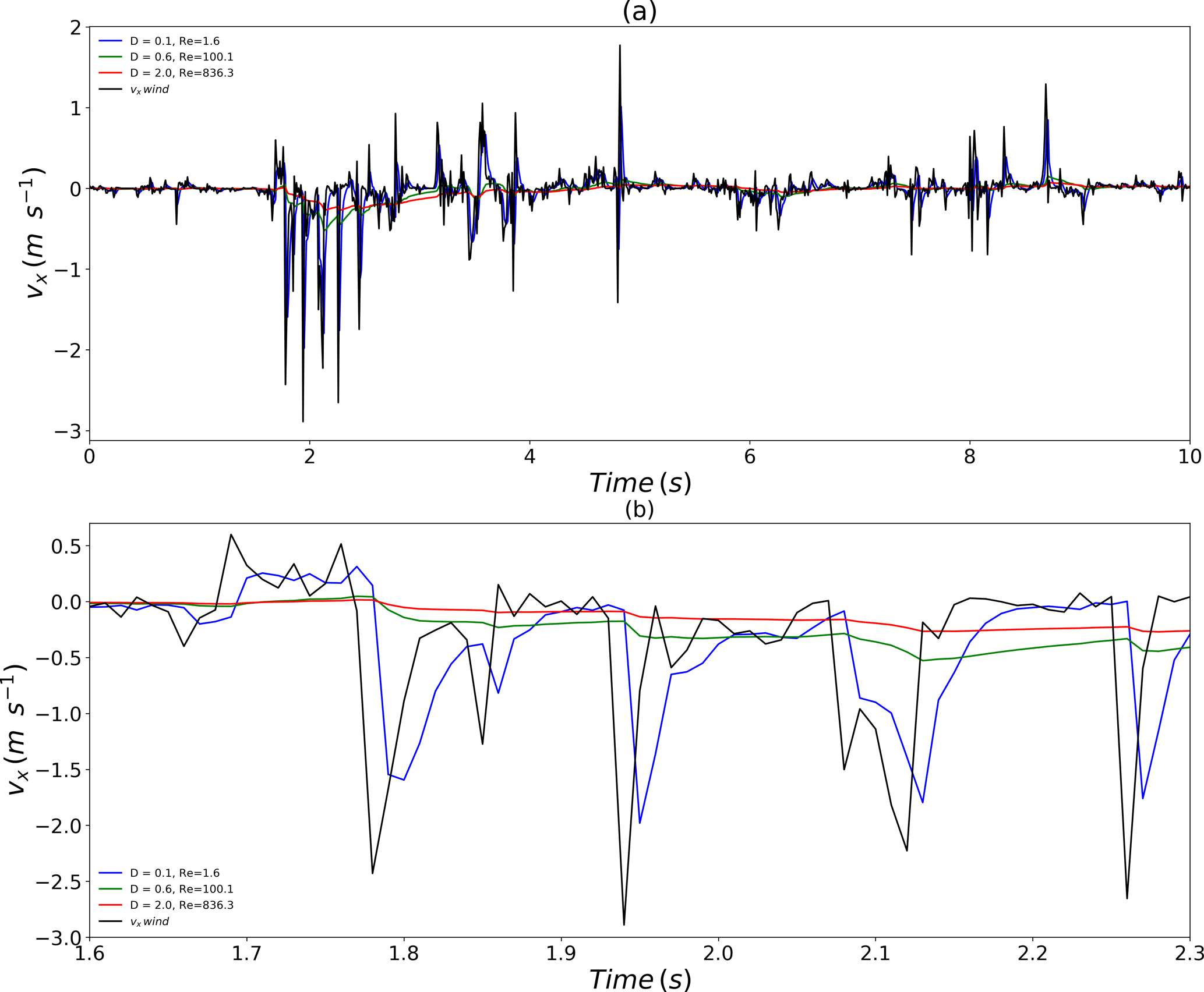
Figure 3(a) Temporal evolution of the drop horizontal velocity during 10 s for various drop diameters (the equivolumic diameter is indicated) with the same multifractal wind input (black). (b) A zoom of the above curve on a shorter period.
In order to quantify this qualitative behaviour more precisely, a multifractal analysis on the retrieved ensembles was performed. Figure 4 displays the outcome of spectral and TM analyses for drops of equivolumic diameter ranging from 0.1 to 2 mm. The spectral analyses reflect a good scaling behaviour over the whole range of scales. Spectral slopes (β in Eq. 8) of 0.86 and 2.25, respectively, are retrieved. For the 2 mm drop, the value corresponds to non-conservative fields. In order to ensure that a conservative field is studied in TM analysis, which is necessary (Lavallée et al., 1993), a fractional differentiation with an exponent is implemented on the field before implementing this TM analysis. TM analysis is displayed in the right-hand column of Fig. 4. For the 0.1 mm drop, an excellent scaling behaviour is retrieved with the coefficient of determination r2 for q=1.5 greater than 0.99. DTM analysis yields estimates of UM parameters α, C1 and H equal to 1.68, 0.21 and 0.12, respectively, which is close to the features of the input series. For the 2 mm drop, the scaling is slightly degraded but remains good (r2=0.95 for q=1.5), and we find α=1.69, C1=0.14 and H=0.79.
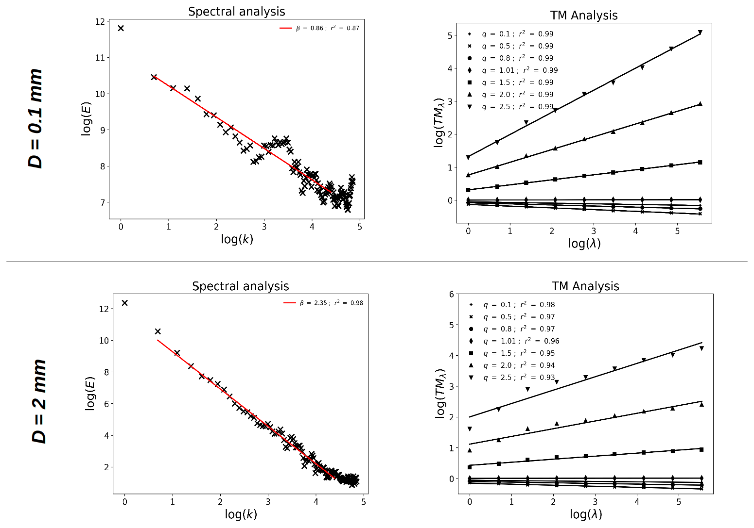
Figure 4Scaling behaviour of the simulated drop velocity for Deq equal to 0.1 mm (top row) and 2 mm (bottom row). Spectral analysis (i.e. Eq. 8 in log–log) on the direct simulations is displayed in the left-hand column. TM analysis (i.e. Eq. 6 in log–log) on the velocity after implementing a fractional integration is displayed in the right-hand column.
Figure 5 displays a summary of the UM analysis carried out on the generated series for the various drops. The scaling behaviour is excellent for small drops and remains good for all drop sizes with r2 for q=1.5 always greater than 0.95 (Fig. 5e). The need for a fractional differentiation before implementing TM analysis is visible with the very poor scaling found when analysing the field directly. The non-conservativeness parameter rapidly increases from 0.1 to 0.8 with the drop size increasing from 0.1 to ≈ 1–1.5 mm. For larger drops, it remains rather stable. This increase of H is basically a quantification of the increased dampening of wind fluctuations observed for larger drops, shown in Fig. 3. With respect to the UM parameters α and C1, the former remains stable and close to the input value of 1.7 for all drop sizes. The latter exhibits a small decrease with larger drops. It should be recalled that this approach is somehow artificial since all drops perceive the same wind, which would not be the case in reality because they do not fall at the same vertical speed. In summary, this investigation shows that horizontal drop velocity basically reproduces the multifractal properties of the wind input with an increased level of non-conservativeness H; H increases strongly for drops smaller than 1 mm and then stabilizes.
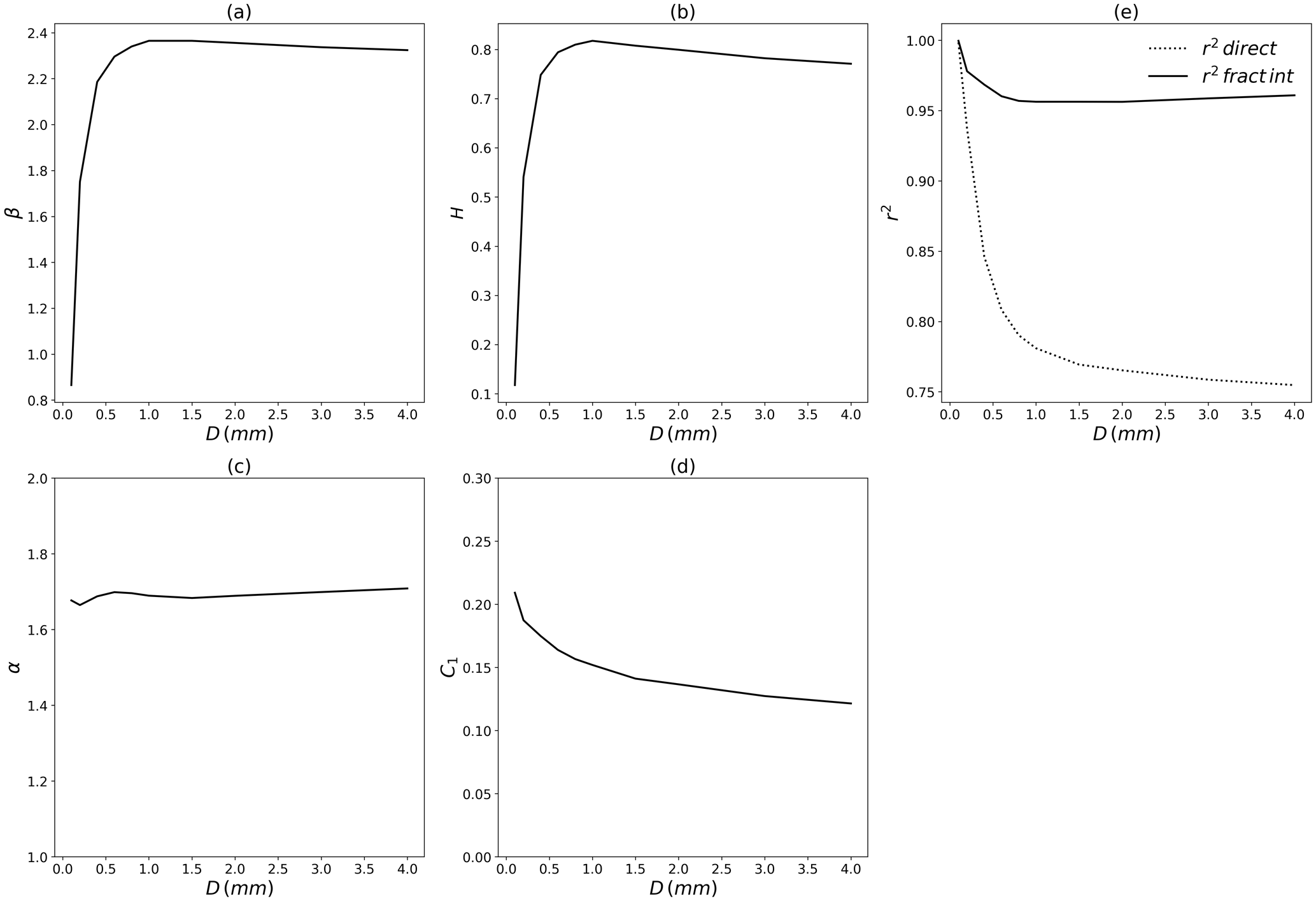
Figure 5Summary of the multifractal analysis performed on the ensembles of simulated horizontal drop velocities using a wind input with α=1.7, C1=0.2. The various multifractal parameters are displayed vs. D (the equivolumic drop diameter).
4.1 Methodology
The purpose of this section is to investigate where drops falling from a height of 1500 m reach the ground. Given the time step of 0.01 s used in the equation and the fact that drops move in space during their fall, this means that it is necessary to have high-resolution space-time 3D wind data over an area of the typical size of a few kilometres to fully address the issue. Such data is unfortunately not available. Hence, we suggest here to reconstruct a somehow realistic wind from a punctual measurement relying on previous findings on turbulence.
4.1.1 Wind data
More precisely, we use 100 Hz 3D sonic anemometer data collected at by a device installed at 78 m on a meteorological mast located on the Pays d'Othe wind farm within the framework of the ANR RW-Turb project. The wind farm is roughly 120 km south-east of Paris on a slightly sloppy area. More details can be found in the data paper under discussion at ESSD (Gires et al., 2022) and in the data set (Gires et al., 2021). Two wind series with very different average horizontal wind speeds (i.e. 1.8 vs. 11.8 m s−1) were extracted for this study. They were later denoted low wind event and strong wind event. The corresponding time series of the three components of the wind for both events are displayed in Fig. 6 over approximately 900 s. The low wind event was collected on 20 January 2021, while the strong one occurred on 6 January 2021.
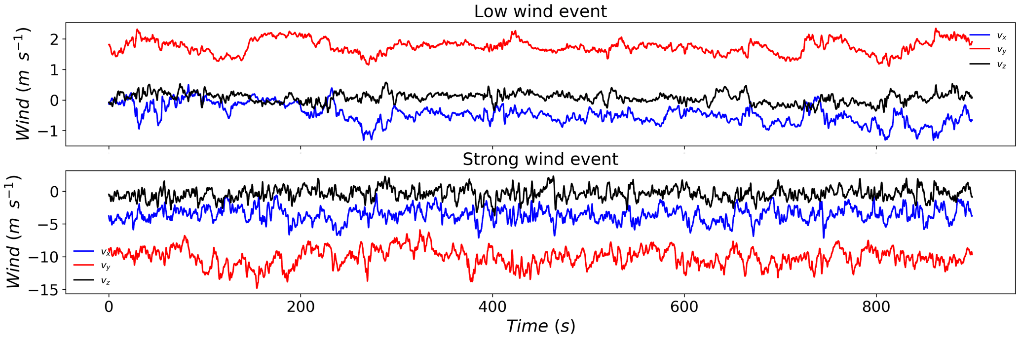
Figure 6Temporal evolution of the 100 Hz wind data from a 3D sonic anemometer for the low (top) and strong (bottom) wind events used in this paper.
4.1.2 Generation of an anisotropic 3D turbulent field
In this section, we discuss how to stochastically generate a turbulent field reproducing the physics of such a flow constraint as well as possible to have the empirical velocity values of the 3D sonic anemometer located at .
Scaling and anisotropy
It is quite obvious that gravity has such a strong impact on drop trajectories and dynamics of drops that classical scaling approaches just fail because they presuppose isotropy. On the contrary, the anisotropy between the vertical and the horizontal induced by gravity is so ubiquitous in geophysics that it has led to the general concept and framework of “generalized scale invariance” for the analysis and simulation of anisotropic fields (Schertzer and Lovejoy, 1985, 1988, 1989; Lazarev et al., 1994; Schertzer et al., 2012), and new extensions have been developed for vector fields (Schertzer and Tchiguirinskaia, 2015, 2020). While classical approaches consider scaling only after assuming isotropy, general scale invariance first posit scaling and then study the remaining non-trivial symmetries. Because this paper deals with scalar discrete cascades, and, therefore, their limitations, we consider an oversimplification of the generalised scale invariance. Recall that for the simplest case of generalised scale invariance, a v horizontal component of a statistically translation invariant velocity field satisfies the following self-affine scale invariance:
where stands for equality in distribution, for a (vector) pair separation, for the induced velocity component shear, Hh for the horizontal scaling exponent ( for Kolmogorov's scaling) and Tλ for a self-affine change of scale:
where G is the generator of Tλ, is the scaling anisotropy exponent and Hv the scaling exponent along the vertical; for a Bolgiano–Obukhov scaling along the vertical, and, therefore, , while for isotropic 3D turbulence . The main property of Tλ is that it broadly generalises in a straightforward manner scales from classical isotropic frameworks (Hz=1) to generalised scales of anisotropic frameworks (e.g. Hz≠1), so that any isotropic cascade can be transformed in this manner into an anisotropic cascade without anything else. Just recall the canonical example of generalised scales for a diagonal generator (p≥1):
which displays the (generalised) scaling property of the generalised scales.
Equation (11) is valid for any direction of (), in particular along the horizontal Δx and the vertical Δz:
which, respectively, can be interpreted as:
with scaling exponents for the kinetic energy flux density ε and for the buoyancy force flux density ϕ. Due to the fact that eddies can be defined as structures having a given velocity shear Δv, we have, in fact, the following balance between both flux densities:
and finally:
due to the respective scaling of the horizontal and vertical eddy sizes defined by the scale change Tλ (Eq. 12).
This confirms that ϕ and ε are both sides of the same coin (Eq. 11). In summary, what is only needed is an anisotropic cascade defined by an anisotropic scale compatible (e.g. Eq. 14) with the anisotropic scale change Tλ (Eq. 12), the intermittency being introduced either by the flux density ε or ϕ (Eq. 15), which respect their equivalence (Eq. 17).
Practical difficulties only occur with discrete scales because they cannot easily deal with arbitrary Hz.
Discrete scales and an ad-hoc approximation
To get around these difficulties, it was tentatively proposed to consider the following 3D model:
where is the (classical), horizontal distance from the anenometer and θ is the buoyancy force flux but is supposed independent of ε contrary to ϕ (Eq. 17). Unfortunately, this model suffers from a number of basic problems:
-
Equalities in distribution are replaced by deterministic equalities, which oversimplify and trivialise the dynamics for each realisation.
-
The flux density ε is defined only along three directions instead along all directions (Eq. 11), whose corresponding components (εx, εy, εz) are supposed to be independent, which is not a tenable assumption.
-
The introduction of θ independent of ε is purely ad hoc to additively(!) introduce a second isotropic scaling (!), and therefore the change of scaling is reduced to a linear cross-over.
-
The scale of the flux densities ε and θ is implicitly taken as the scale of the simulation resolution instead of the pair separation scale (Eq. 15). The resulting mismatch between both scales will introduce a statistical bias.
-
Moreover, the density values are arbitrarily taken at the locations ( for ε) and z+Δz for θ. This introduces a dissymmetry that is not without consequences.
-
All time steps are fully independent, with the exception of the empirical velocity values measured by the 3D sonic anemometer.
The limitations of this model are, therefore, extremely strong. Many of them would have been resolved with the help of the scalar anisotropic cascades recalled above (see the previous paragraph). But to fully overcome them would require us to consider their extension to vector fields (Schertzer and Tchiguirinskaia, 2015, 2020). This remains outside the scope of this paper, and this simplistic approach is used for a sort of exploratory step focused on the interaction of drops and a given velocity field. The results obtained, therefore, have to be critically examined, since many of them are sensitive to the aforementioned oversimplifications.
4.1.3 Practical implementation
The fields ϵ (i.e. the ones for the horizontal shift) are simulated in space time with a size using discrete UM cascades and Eq. (10) to obtain either positive or negative values. The number 729 refer to space, while 64 refers to time. Before stating the physical resolution of the field, it should be explained that a simple anisotropy between space and time is accounted through a scaling anisotropy coefficient Ht. Within such framework, when the spatial scale of the data is changed by a ratio of λxy, the temporal scale should be changed by a factor of ; Ht is expected to be equal to (Marsan et al., 1996), hence when the spatial scale is multiplied by 3, the temporal scale should be multiplied by 2 (i.e. ) (Biaou et al., 2005; Gires et al., 2014). These fields are assumed to cover an area of the size 40 km × 40 km × 1024 s, which is needed for drift of 0.1 mm drops during their fall when wind is strong. This means that a voxel is of size 53 m × 53 m × 16 s.
The fields θ (i.e. those for the vertical shift) are of size 512×64 covering a physical are of 1600 m × 1024 s, meaning a pixel size 3 m × 16 s. All UM fields are simulated with α=1.7, C1=0.2, as in the previous section.
Finally, at any point a bi or tri-linear interpolation is implemented to obtain the value of the field from the nearest points. The value of the prefactor were set to , and through an heuristic approach of trial and error to get some realistic fluctuations. In the future, it would obviously be necessary to tune them to local wind properties. However, such tuning is outside the scope of this section, which aims more at being a proof of concept.
4.2 Illustration
In order to illustrate the suggested process, let us consider a 0.5 mm drop during the low wind event. Its initial position is in m. It is “dropped” with no horizontal velocity and a vertical velocity equal to that of its terminal. The anemometer is assumed to be located at m. Then Eq. (5) is implemented. At each time step, the local wind is assessed using the methodology described in the previous paragraphs.
The actual total wind perceived by the drop (i.e. the input in Eq. 5) is recorded and displayed in last row of Fig. 7. It corresponds to the sum of the wind from the anemometer (the first row in Fig. 7) plus a wind shift field (the middle row in Fig. 7). This leads to a given trajectory in space, which is shown in Fig. 8. The projected trajectory on the planes (x,y) and (x,z) is also shown. This trajectory exhibits a nonlinear complex pattern, which results from the turbulent nature of the wind. It should be mentioned that not accounting for oblateness affects not only the vertical velocity but the whole trajectory as well. Depending on the model (spheres or oblate drops), shifts of more than few hundred metres are found even for large drops for some events.
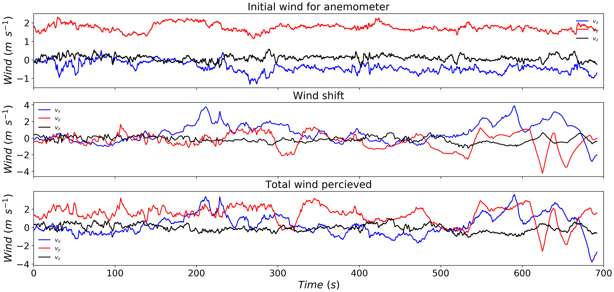
Figure 7(Top) Temporal evolution with 0.01 s time steps of the wind data from 3D sonic anemometer, (middle) the wind shift and (bottom) the total wind perceived by the 0.5 mm drop falling from the position during the low wind event. Bottom panel is actually the wind input used to obtain the trajectory of Fig. 8.
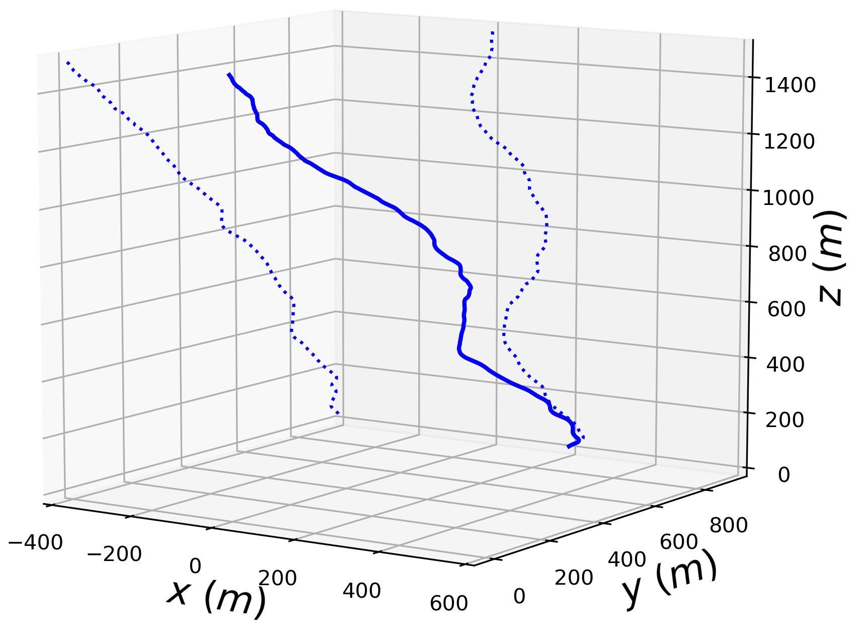
Figure 8Trajectory (solid line) of a 0.5 mm drop in a turbulent wind field for the low wind event. The dotted lines correspond to the trajectory projected on the (x,z) and (y,z) plane.
4.3 Sensitivity to the wind shift field
The process to generate an estimation of a 3D wind field is actually stochastic through the UM fields ϵ and θ used in Eq. (18). In this section, the sensitivity to the given realization of the process is discussed. In order to achieve that, 10 wind samples are generated with the same input parameters (described in Sect. 4.1) and the corresponding trajectories for drops of size 0.5, 1, 2 and 3 mm are computed.
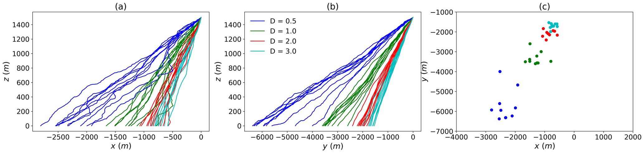
The projected trajectories for the low wind event, are displayed in Fig. 9a and b. The position of the dropa when they reach the ground is shown in Fig. 9c. The spread of the drops strongly depends on their size, with a decrease as the drop size increases. Indeed, Δx (xmax−xmin) is equal to 1238, 591, 415 and 404 m for drops of sizes 0.5, 1, 2 and 3 mm, respectively. For Δy, the values are 2123, 897, 461 and 322 m. Such a decrease is due to a combination of the fact that smaller drops are more subject to wind fluctuations (Sect. 3) and that they spend more time in the atmosphere (Sect. 2) before they reach the ground. Similar trends are retrieved for the strong wind event (Fig. 10) with a stronger absolute shift. In that case, the values for Δx are 890, 868, 500 and 448 m, respectively. For Δy, they are 2382, 1003, 568 and 448 m.
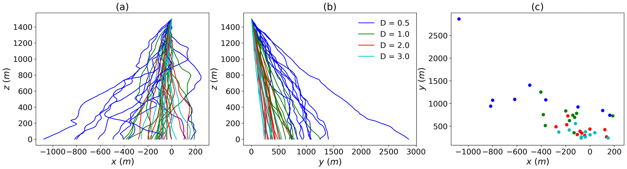
Figure 9(a, b) Trajectories of drops of various sizes falling from the position, projected on the (x,z) and (y,z) plane, respectively. The low wind event is used. The ten curves correspond to different realizations of the wind shift field. (c) Position of the ground impact of the various drops.
4.4 Illustration of impact on rainfall retrieval with weather radars
In this last section, initial investigations toward understanding the consequence of previous work on quantitative rainfall measurement with weather radars are carried out. Indeed, weather radar measure rainfall at a given altitude, while hydro-meteorologists are interested in rainfall at ground level. During their fall, significant shifts can occur. In order to study it, the following process is implemented. For 5 min, one rainfall drop is dropped every 15 s from a random position within a voxel of size 100 m centred on m. Hence it covers a total duration of 5 min. The trajectories and positions on the ground of the drops is then studied. This enables us to basically mimic the measurement of a weather radar at its typical gate size and temporal resolution.
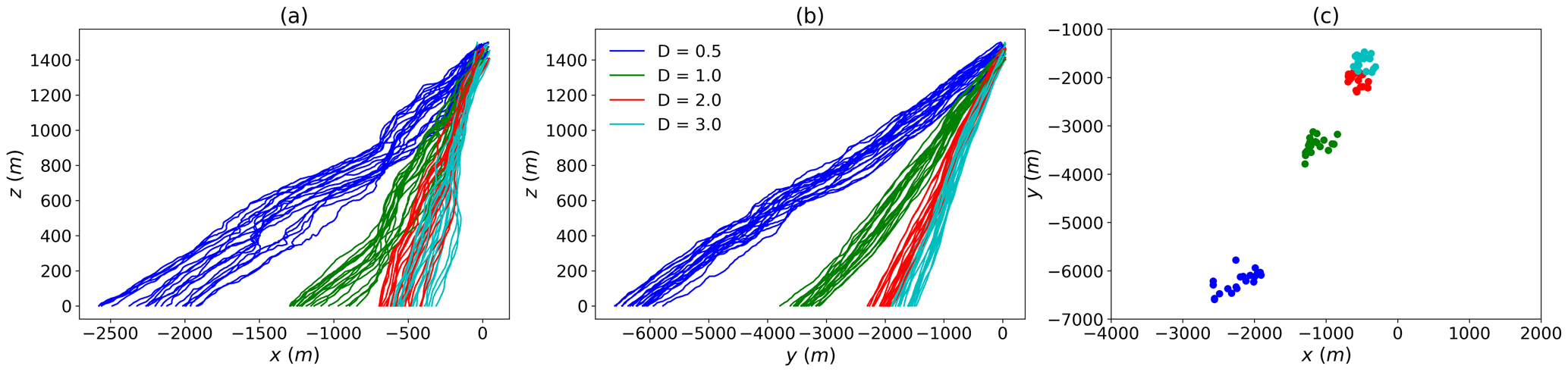
Figure 11 displays the trajectories and ground impact location in the case of the low wind event for a given realisation of the stochastic wind shift. A shift of more than 1 km for small drops is found, and more than 300 m for 3 mm drops. As noted in the previous section, the spread of drops at ground level tends to decrease with increasing drop size. Indeed, Δx (xmax−xmin) is equal to 206, 119, 165 and 121 m for drop of sizes 0.5, 1, 2 and 3 mm, respectively. For Δy, the values are 184, 134, 112 and 88 m. For the strong wind event (Fig. 12), shifts of more than 6 and 1.5 km are reported for drops of size 0.5 and 3 mm respectively. Similar results as for the low wind event are found with regards to the spread. The corresponding figures are of 665, 450, 284 and 307 m for Δx, and of 819, 664, 429 and 420 m for Δy.
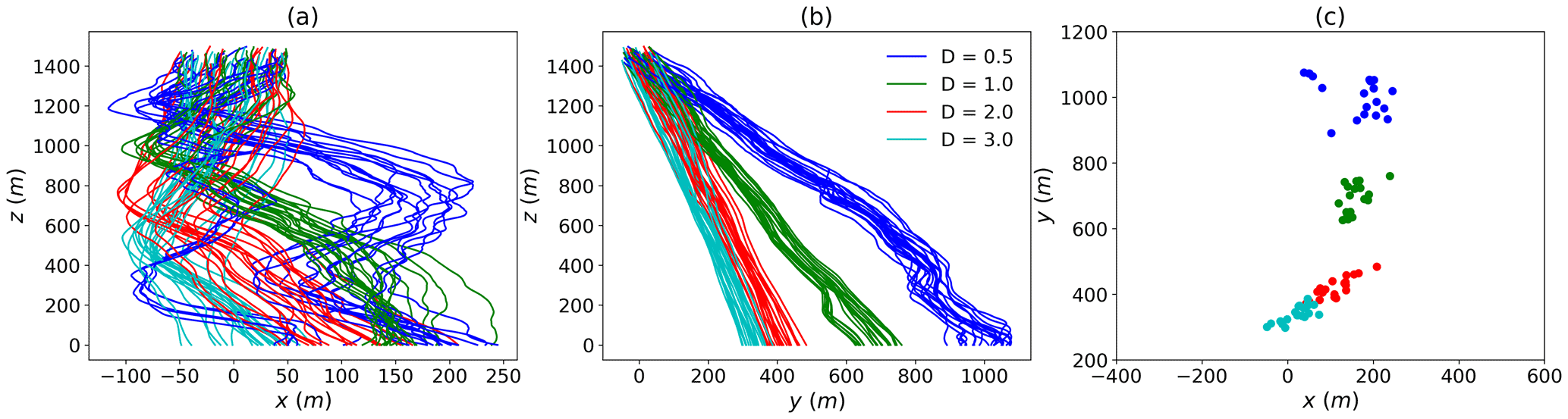
Figure 11(a, b) Trajectories of drops of various sizes falling from a 100 m cubic voxel centred on a position, projected on the (x,z) and (y,z) plane, respectively. The low wind event is used. For each size, the 20 drops are dropped every 15 s (hence over a total duration of 5 min). A single realization of the wind shift field is used. (c) Position of the ground impact of the various drops.
As was previously pointed out, this spread is due to the fact that smaller drops spend more time in the atmosphere and are more sensitive to wind fluctuations. Indeed, the duration of a fall from 1500 m to the ground at 0 m is equal to 716, 378, 238 and 192 s for drops of size 0.5, 1, 2 and 3 mm, respectively. Given that high-resolution radar pixels are typically of the size of a few hundred metres, one should note that drops within a given voxel at measurement height can reach the ground within an area of size 3 km × 6 km. Even within a drop diameter class, shifts are of few radar pixels. Given that drop size distribution also varies, such a shift can significantly affect rainfall retrieval, even in low wind conditions.
In this paper, we have aimed for a better understanding of the behaviour of individual rainfall drops falling from typically 1500 m. In a first step, we developed a new approach to compute the drag coefficient accounting for drop oblateness and findings in fluid mechanics. This was validated for drops of equivolumic size of up to 4 mm through the comparison between the retrieved terminal fall velocity and the commonly used formula.
Then the temporal evolution of the horizontal drop velocity under turbulent wind constraints was studied. It appears that multifractal features of the input wind are simply transferred to drop velocity with an additional fractional integration and slight time shift. The UM parameters α and C1 are basically conserved, while H is increased. The increase ranges from 0.1 for 0.1 mm size drops to 0.8 for 1–1.5 mm size drops. It remains rather constant for larger drops.
Finally, the trajectories of drops of various sizes falling form 1500 m was studied as a proof of concept. For this, 100 Hz anemometer data was used, and an approach to simulate realistic fluctuations of wind in space was developed. It notably enables to analyse how drop shift during their fall between their location measurement by weather radars and ground impact. For a strong wind event, drops located within a radar gate in altitude for 5 min are spread on the ground over an area of a few kilometres. The spread for drops of a given diameter is found to cover a few radar pixels.
In order to further explore the consequences of these findings on quantitative rainfall estimation with weather radars, further investigations are needed. More precisely, (i) the model to simulate wind fluctuations should be improved, notably to use vector simulations and tune the prefactors according to local wind conditions; (ii) space-time outputs of numerical weather prediction models could also be tested to retrieve wind fields; (iii) the actual drop size distribution should be used to better assess the impact for the ground estimation of precipitation, which implies making some simulations for a much larger number of drops; (v) a longer period of time should be tested to investigate where the water volume (i.e. all the drops) of a given radar gate fall during an event. For the two last points, data is available within the RW-Turb project. Such step would then need to be repeated over various radar gates to derive updated radar maps. Given the limited computation power that will not allow us to simulate the trajectories of all the drops, some statistical behaviour according to each radar gate and wind conditions would need to be designed and then computed. It should also be stressed that only individual drops are currently being handled. This means that the methodology developed does not account for either collision, aggregation between drops or for breakup. Such processes are also known to affect drop velocities by changing their size and shape. Future investigations should also aim at accounting for them. Finally, it should also be stressed that the method developed stochastically simulates wind fluctuations at small scales. This means that the output will not be a deterministic radar measurement but an ensemble of possible realistic outputs, out of which a probability distribution could be derived. Such a probabilistic approach is discussed in Kirstetter et al. (2015) with a focus on intrinsic radar uncertainties and not wind drift.
The algorithms used in this paper were developed in Python programming language and can be obtained from the authors on request.
Wind data used in this paper can be found at https://doi.org/10.5281/zenodo.5801900 (Gires et al., 2021). The description of the data set can be found in Gires et al. (2022, https://doi.org/10.5194/essd-14-3807-2022).
All authors designed the structure and main content of the paper. AG performed the numerical simulations and wrote most of the text. DS and IT identified and highlighted the limitations of the current modelling and outlined perspectives to overcome them. All authors contributed to the revision of the paper.
The contact author has declared that none of the authors has any competing interests.
Publisher's note: Copernicus Publications remains neutral with regard to jurisdictional claims in published maps and institutional affiliations.
The authors gratefully acknowledge partial financial support from the Chair “Hydrology for Resilient Cities” (endowed by Veolia) of Ecole des Ponts ParisTech, the Île-de-France region RadX@IdF Project.
This research has been supported by the ANR JCJC RW-Turb project (grant no. ANR-19-CE05-0022).
This paper was edited by Alexis Berne and reviewed by Miguel Angel Rico-Ramirez and one anonymous referee.
Atlas, D., Srivastava, R. C., and Sekhon, R. S.: Doppler radar characteristics of precipitation at vertical incidence, Rev. Geophys., 11, 1–35, https://doi.org/10.1029/RG011i001p00001, 1973. a
Bagheri, G.: Numerical and experimental investigation of particle terminal velocity and aggregation in volcanic plumes, Thèse de doctorat no. Sc. 4844, PhD thesis, Université de Genève, https://doi.org/10.13097/archive-ouverte/unige:77593, 2015. a
Beard, K. V.: Terminal velocity adjustment for cloud and precipitation aloft, J. Atmos. Sci, 34, 1293–1298, 1977. a
Best, A. C.: Empirical formulae for the terminal velocity of water drops falling through the atmosphere, Q. J. Roy. Meteor. Soc., 76, 302–311, https://doi.org/10.1002/qj.49707632905, 1950. a
Biaou, A., Chauvin, F., Royer, J.-F., and Schertzer, D.: Analyse multifractale des précipitations dans un scénario GIEC du CNRM, Note de centre GMGEC, CNRM, Vol. 101, 2005. a
Blocken, B., Stathopoulos, T., Carmeliet, J., and Hensen, J. L.: Application of computational fluid dynamics in building performance simulation for the outdoor environment: an overview, J. Build. Perform. Simu., 4, 157–184, https://doi.org/10.1080/19401493.2010.513740, 2011. a
Bringi, V., Thurai, M., and Baumgardner, D.: Raindrop fall velocities from an optical array probe and 2-D video disdrometer, Atmos. Meas. Tech., 11, 1377–1384, https://doi.org/10.5194/amt-11-1377-2018, 2018. a
Collier, C.: The impact of wind drift on the utility of very high spatial resolution radar data over urban areas, Phys. Chem. Earth Pt. B, 24, 889–893, https://doi.org/10.1016/S1464-1909(99)00099-4, 1999. a
Dai, Q., Han, D., Rico-Ramirez, M. A., and Islam, T.: The impact of raindrop drift in a three-dimensional wind field on a radar–gauge rainfall comparison, Int. J. Remote Sens., 34, 7739–7760, https://doi.org/10.1080/01431161.2013.826838, 2013. a
Dai, Q., Yang, Q., Han, D., Rico-Ramirez, M. A., and Zhang, S.: Adjustment of Radar-Gauge Rainfall Discrepancy Due to Raindrop Drift and Evaporation Using the Weather Research and Forecasting Model and Dual-Polarization Radar, Water Resour. Res., 55, 9211–9233, https://doi.org/10.1029/2019WR025517, 2019. a
Fitton, G., Tchiguirinskaia, I., Schertzer, D., and Lovejoy, S.: Scaling Of Turbulence In The Atmospheric Surface-Layer: Which Anisotropy?, J. Phys. Conf. Ser., 318, 072008, https://doi.org/10.1088/1742-6596/318/7/072008, 2011. a
Gires, A., Tchiguirinskaia, I., Schertzer, D., Schellart, A., Berne, A., and Lovejoy, S.: Influence of small scale rainfall variability on standard comparison tools between radar and rain gauge data, Atmos. Res., 138, 125–138, https://doi.org/10.1016/j.atmosres.2013.11.008, 2014. a
Gires, A., Tchiguirinskaia, I., and Schertzer, D.: Blunt extension of discrete universal multifractal cascades: development and application to downscaling, Hydrolog. Sci. J., 65, 1204–1220, https://doi.org/10.1080/02626667.2020.1736297, 2020. a
Gires, A., Jose, J., Tchiguirinskaia, I., and Schertzer, D.: Data for: “Three months of combined high resolution rainfall and wind data collected on a wind farm”, Zenodo [data set], https://doi.org/10.5281/zenodo.5801900, 2021. a, b
Gires, A., Jose, J., Tchiguirinskaia, I., and Schertzer, D.: Combined high-resolution rainfall and wind data collected for 3 months on a wind farm 110 km southeast of Paris (France), Earth Syst. Sci. Data, 14, 3807–3819, https://doi.org/10.5194/essd-14-3807-2022, 2022. a, b
Hölzer, A. and Sommerfeld, M.: New simple correlation formula for the drag coefficient of non-spherical particles, Powder Technol., 184, 361–365, https://doi.org/10.1016/j.powtec.2007.08.021, 2008. a, b
Kirstetter, P.-E., Gourley, J. J., Hong, Y., Zhang, J., Moazamigoodarzi, S., Langston, C., and Arthur, A.: Probabilistic precipitation rate estimates with ground-based radar networks, Water Resour. Res., 51, 1422–1442, https://doi.org/10.1002/2014WR015672, 2015. a
Kruger, A. and Krajewski, W. F.: Two-Dimensional Video Disdrometer: A Description, J. Atmos. Ocean. Tech., 19, 602–617, https://doi.org/10.1175/1520-0426(2002)019<0602:TDVDAD>2.0.CO;2, 2002. a
Lack, S. A. and Fox, N. I.: An examination of the effect of wind-drift on radar-derived surface rainfall estimations, Atmos. Res., 85, 217–229, https://doi.org/10.1016/j.atmosres.2006.09.010, 2007. a, b, c
Lauri, T., Koistinen, J., and Moisseev, D.: Advection-Based Adjustment of Radar Measurements, Mon. Weather Rev., 140, 1014–1022, https://doi.org/10.1175/MWR-D-11-00045.1, 2012. a, b
Lavallée, D., Lovejoy, S., and Ladoy, P.: Nonlinear variability and landscape topography: analysis and simulation, in: Fractas in geography, edited by: de Cola, L. and Lam, N., Prentice-Hall, 171–205, ISBN 9780131058675, 1993. a, b
Lazarev, A., Schertzer, D., Lovejoy, S., and Chigirinskaya, Y.: Unified multifractal atmospheric dynamics tested in the tropics: part II, vertical scaling and generalized scale invariance, Nonlin. Processes Geophys., 1, 115–123, https://doi.org/10.5194/npg-1-115-1994, 1994. a
Lhermitte, R. M.: Cloud and precipitation remote sensing at 94 GHz, IEEE T. Geosci. Remote, 26, 207–216, 1988. a
Marsan, D., Schertzer, D., and Lovejoy, S.: Causal space-time multifractal processes: Predictability and forecasting of rain fields, J. Geophys. Res., 101, 26333–26346, 1996. a
Mittermaier, M. P., Hogan, R. J., and Illingworth, A. J.: Using mesoscale model winds for correcting wind-drift errors in radar estimates of surface rainfall, Q. J. Roy. Meteor. Soc., 130, 2105–2123, https://doi.org/10.1256/qj.03.156, 2004. a
Montero-Martínez, G. and García-García, F.: On the behaviour of raindrop fall speed due to wind, Q. J. Roy. Meteor. Soc., 142, 2013–2020, 2016. a
Pedersen, H. S. and Hasholt, B.: Influence of wind speed on rainsplash erosion, CATENA, 24, 39–54, https://doi.org/10.1016/0341-8162(94)00024-9, 1995. a
Sandford, C.: Correcting for wind drift in high resolution radar rainfall products: a feasibility study, J. Hydrol., 531, 284–295, https://doi.org/10.1016/j.jhydrol.2015.03.023, 2015. a
Schertzer, D. and Lovejoy, S.: The dimension and intermittency of atmospheric dynamics, in: Turbulent shear flow 4. Selected papers from the Fourth International Symposium on “Turbulent Shear Flow”, edited by: Bradbury, L. J. S., Durst, F., Launder, E., Schmidt, F. W., and Whitelaw, J. H., Springer-Verlag, Berlin, 7–33, ISBN 9783642699986, 1985. a
Schertzer, D. and Lovejoy, S.: Physical modelling and analysis of rain and clouds by anisotropic scaling and multiplicative processes, J. Geophys. Res., 92, 9693–9714, 1987. a
Schertzer, D. and Lovejoy, S.: Nolinear variability in geophysics multifractal analysis and simulations, in: Fractals Physical Origin and properties, edited by: Pietronero, L., Plenum Press, New-York, 41–82, ISBN-13: 978-0306434136, ISBN-10: 030643413X, 1988. a
Schertzer, D. and Lovejoy, S.: Generalised scale invariance and multiplicative processes in the atmosphere, Pure Appl. Geophys., 130, 57–81, https://doi.org/10.1007/BF00877737, 1989. a
Schertzer, D. and Lovejoy, S.: From scalar cascades to lie cascades: joint multifractal analysis of rain and cloud processes, in: Space/time variability and interdependence for various hydrological processes, edited by: Feddes, R., Cambridge University Press, 153–173, ISBN 9780521495080, 1995. a
Schertzer, D. and Lovejoy, S.: Universal multifractals do exist!: Comments, J. Appl. Meteorol., 36, 1296–1303, https://doi.org/10.1175/1520-0450(1997)036<1296:UMDECO>2.0.CO;2, 1997. a
Schertzer, D. and Tchiguirinskaia, I.: Multifractal vector fields and stochastic Clifford algebra, Chaos, 25, 123127, https://doi.org/10.1063/1.4937364, 2015. a, b
Schertzer, D. and Tchiguirinskaia, I.: A Century of Turbulent Cascades and the Emergence of Multifractal Operators, Earth and Space Science, 7, e2019EA000608, https://doi.org/10.1029/2019EA000608, 2020. a, b, c, d
Schertzer, D., Tchiguirinskaia, I., Lovejoy, S., and Tuck, A. F.: Quasi-geostrophic turbulence and generalized scale invariance, a theoretical reply, Atmos. Chem. Phys., 12, 327–336, https://doi.org/10.5194/acp-12-327-2012, 2012. a
Stout, J. E., Arya, S. P., and Genikhovich, E. L.: The Effect of Nonlinear Drag on the Motion and Settling Velocity of Heavy Particles, J. Atmos. Sci., 52, 3836–3848, https://doi.org/10.1175/1520-0469(1995)052<3836:TEONDO>2.0.CO;2, 1995. a, b, c
Thurai, M., Huang, G. J., Bringi, V. N., Randeu, W. L., and Schönhuber, M.: Drop Shapes, Model Comparisons, and Calculations of Polarimetric Radar Parameters in Rain, J. Atmos. Ocean. Tech., 24, 1019–1032, https://doi.org/10.1175/JTECH2051.1, 2007. a, b
Thurai, M., Schönhuber, M., Lammer, G., and Bringi, V.: Raindrop shapes and fall velocities in “turbulent times”, Adv. Sci. Res., 16, 95–101, https://doi.org/10.5194/asr-16-95-2019, 2019. a
Tian, L., Zeng, Y.-J., and Fu, X.: Velocity Ratio of Wind-Driven Rain and Its Application on a Transmission Tower Subjected to Wind and Rain Loads, J. Perform. Constr. Fac., 32, 04018065, https://doi.org/10.1061/(ASCE)CF.1943-5509.0001210, 2018. a
White, F.: Viscous Fluid Flow, McGraw-Hill, ISBN 0-07-069712-4, 1974. a
Yang, Q., Dai, Q., Han, D., Zhu, Z., and Zhang, S.: Uncertainty analysis of radar rainfall estimates induced by atmospheric conditions using long short-term memory networks, J. Hydrol., 590, 125482, https://doi.org/10.1016/j.jhydrol.2020.125482, 2020. a
- Abstract
- Introduction
- A deterministic equation for oblate drops in a wind field
- Behaviour of horizontal drop velocity with multifractal input
- Ground impact location of drops falling in a turbulent wind field
- Conclusions
- Code availability
- Data availability
- Author contributions
- Competing interests
- Disclaimer
- Acknowledgements
- Financial support
- Review statement
- References