the Creative Commons Attribution 4.0 License.
the Creative Commons Attribution 4.0 License.
 | 25 Oct 2022
An improved OSIRIS NO2 profile retrieval in the upper troposphere–lower stratosphere and intercomparison with ACE-FTS and SAGE III/ISS
Daniel Zawada
Adam Bourassa
Doug Degenstein
William Randel
David Flittner
Patrick Sheese
Kaley Walker
The v7.2 NO2 retrieval for the Optical Spectrograph and InfraRed Imager System (OSIRIS) was designed to improve sensitivity in the upper troposphere–lower stratosphere (UTLS) and to reduce an observed low bias in the previous version, v6.0. The details of this retrieval are described and then the data are compared to coincident NO2 profiles from the Atmospheric Chemistry Experiment–Fourier Transform Spectrometer (ACE-FTS) and the Stratospheric Aerosol and Gas Experiment III on the International Space Station (SAGE III/ISS). The PRATMO photochemical box model was used to account for differences in the measurement times of the instruments: all datasets were scaled to the same local solar time of 12:00 LST. Coincident ACE-FTS and OSIRIS NO2 measurements agree within 20 % throughout much of the stratosphere. Coincident SAGE III/ISS and OSIRIS NO2 measurements also agree within 20 %, with OSIRIS biased low at all altitudes and latitudes. The ACE-FTS, OSIRIS, and SAGE III-ISS NO2 monthly zonal mean data show very similar variability in time at most altitude and latitudes.
- Article
(8767 KB) - Full-text XML
- BibTeX
- EndNote


Satellite observations are crucial for monitoring changes in atmospheric composition. Measurements of stratospheric NO2 in particular are important as NO2 is a key factor for ozone photochemistry. It is often necessary to use data from multiple instruments in order to fully explain the distribution of NO2 throughout the stratosphere, but such studies require detailed understanding of the biases between the different datasets. This can be challenging in the case of NO2, where a complex daily photochemical cycle prevents the direct comparison of measurements taken at different local solar times (LSTs). Here we focus on NO2 retrieved from limb scatter and solar occultation instruments. These measurements have excellent vertical resolution, making it possible to study variations in NO2 from the upper troposphere to the mid-stratosphere.
Updated NO2 retrievals were recently developed for several instruments: the Optical Spectrograph and InfraRed Imager System (OSIRIS, Llewellyn et al., 2004), the Atmospheric Chemistry Experiment–Fourier Transform Spectrometer (ACE-FTS, Bernath et al., 2005), and the Stratospheric Aerosol and Gas Experiment on the International Space Station (SAGE III/ISS, Cisewski et al., 2014). OSIRIS takes limb scatter measurements near 06:30 LT (local time, descending node), while ACE-FTS and SAGE III/ISS use the solar occultation technique, with measurements at sunrise and sunset. The latest OSIRIS NO2 retrieval, v7.2, was designed to fix a low bias and to improve performance in the UTLS (upper troposphere–lower stratosphere) through better cloud and aerosol filtering. This retrieval is discussed in detail in Sect. 2. The v7.2 data are then compared to coincident NO2 profiles from ACE-FTS and SAGE III/ISS. The PRATMO photochemical box model, developed by Prather and Jaffe (1990) and updated by McLinden et al. (2000) and later Adams et al. (2017), is used to account for the different instrument measurement times. The ACE-FTS and SAGE III/ISS data are described in Sect. 3, and the results of the comparison are given in Sect. 4.
2.1 The OSIRIS instrument
OSIRIS has been operating from a sun-synchronous orbit on the Odin satellite since October 2001 (Murtagh et al., 2002; Llewellyn et al., 2004). The optical spectrograph measures 100 to 400 vertical profiles of limb-scattered solar irradiance each day, at wavelengths from 275 to 810 nm. Only the descending-phase measurements are used here because the ascending-phase measurements have inconsistent sampling due to drifts in the orbit. The equatorial crossing of the descending phase occurs near 06:30 LST, although the exact timing varies by approximately 1 h due to the spacecraft orbit.
2.2 Prior data versions
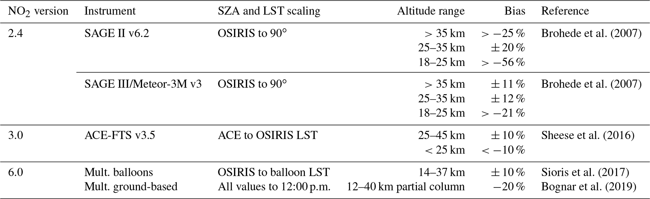
The initial OSIRIS NO2 retrieval was described by Sioris et al. (2003). Subsequent versions of the retrieval were developed by Haley et al. (2004) (v2.4), Haley and Brohede (2007) (v3.0), Bourassa et al. (2011) (“fast” version), and Sioris et al. (2017) (v6.0). Validation studies for previous versions of the OSIRIS retrieval accounted for the NO2 daily photochemical cycle in different ways and found mixed results. A summary of the validation results for the earlier OSIRIS NO2 retrieval versions is provided in Table 1. In general the retrieved OSIRIS v3.0 and v6.0 NO2 values were biased low compared to other instruments, although the bias varies with altitude.
Brohede et al. (2007)Brohede et al. (2007)Sheese et al. (2016)Sioris et al. (2017)Bognar et al. (2019)Table 1Summary of validation results for prior versions of the OSIRIS NO2 retrieval. The SZA and LST scaling column describes how the different measurement times of the instruments were accounted for. A negative bias means that OSIRIS is biased low.
2.3 OSIRIS v7.2 algorithm description
The core of the algorithm is a spectral fit to high-altitude normalized radiances in the 434.8–476.7 nm spectral region,
where Ij(λ) is the OSIRIS-measured radiance at tangent altitude index j and wavelength λ; and are the ozone and nitrogen-dioxide cross sections at the measurement tangent altitude,; and Aj, Bj, Cj, Dj, Ej, and yj are coefficients determined through a linear regression. Ej and yj are related to the slant path optical depths. The ozone cross sections of Daumont et al. (1992), Brion et al. (1993), and Malicet et al. (1995) are used, with the NO2 cross sections taken from Vandaele et al. (1998). The forward model radiative transfer calculation includes the full temperature dependence at all altitudes and the regression for each line of sight uses the temperature at the tangent point to compute the cross section. Both sets of cross sections are sampled at the native resolution of the spectroscopic measurements (typically ∼ 0.02 nm) and then convolved to the OSIRIS measurement spectral resolution (1 nm). A discussion on the stability of the spectral resolution is given in Bognar et al. (2022). The cross section temperature is that at the tangent altitude, where most of the absorption occurs, so the cross section is slightly different for each line of sight. The output of the spectral fitting is the vector , which is then used to represent the observed values in the iterative equation,
where x is a vector of NO2 number density on a 1 km vertical grid with length n, K is the Jacobian matrix , Sy is the covariance matrix of y, xa is the a priori state, R is a regularization matrix, γ is the Levenberg–Marquardt damping parameter, and F is the forward model. The lowest retrieved altitude is determined from the cloud detection performed in the OSIRIS v7.0 aerosol retrieval (Rieger et al., 2019), and the highest altitude extends to 40 km. The forward model is a combination of the SASKTRAN radiative transfer model (Bourassa et al., 2008; Zawada et al., 2015) and the application of Eq. (1). Included in the forward model calculation are the results from the OSIRIS v7.2 ozone, stratospheric aerosol, and surface albedo retrievals. The measurement covariance is assumed to be diagonal and determined through the residuals of the linear regression procedure. A second-derivative Tikhonov-style regularization matrix is used which is scaled by the prior state,
where α is a scale factor, Γ is a numerical second-derivative operator of size , and is the element-wise inverse of xa. The prior state is calculated from a latitude- and month-dependent climatology computed through the box model of Prather and Jaffe (1990).
Convergence is detected through analysis of the quantity being minimized,
The predicted value of χ2, assuming the problem is linear, can be evaluated as follows:
where Δxl,i is found by setting γ=0 in Eq. (2) and evaluating . The iteration is then stopped when
which results in profiles that have converged to a level orders of magnitude less than the estimated precision. Scans where this criteria is not achieved are flagged and discarded.
For each scan, various error characterization metrics are also calculated. The covariance of the retrieved state is calculated as follows:
with the gain matrix G given by
The averaging kernel is computed through
To determine the optimal regularization scale factor, α in Eq. (3), an analysis was performed on representative OSIRIS scans. Regularization scale factor values that are too high result in averaging kernels that are not sharply peaked in the UTLS with degraded vertical resolution, while values that are too low can lead to over-fitting, oscillations, and poor convergence. Figure 1 shows an example of these tests for one OSIRIS scan and three different values of the regularization scale parameter (1, 5, 20). For α=1, we see large oscillations in the UTLS leading to highly negative values. At α=20 the oscillations are damped; however, the response in the UTLS is greatly damped, with poorer vertical resolution in the stratosphere and worse agreement between the OSIRIS measurements and the forward model, particularly above 30 km. At α=5 there is a balance between the oscillations and response and this value maintains a vertical resolution of 2–3 km in most of the stratosphere, which matches the vertical OSIRIS sampling resolution. For these reasons the v7.2 processing uses a regularization value of α=5.

Figure 1Retrieved NO2 and diagnostic information for three different regularization scale values for OSIRIS scan 32921024 (8 March 2007, 23.9∘ N). (a) The retrieved NO2 profile (solid lines) and 1σ error estimates (shaded areas) for three regularization values. (b) The estimated vertical resolution of the retrieval for three regularization values. (c) The ratio of the OSIRIS measurement vector to the simulated measurement vector for three regularization values. (d–f) The averaging kernels for the three regularization values.
2.4 Comparison to OSIRIS v6.0
The v6.0 algorithm uses a similar procedure where the measurement vector is determined from the regression fit in Eq. (1), but v7.2 makes key improvements aimed to reduce the observed low biases and improve the knowledge of the response in the UTLS. A full description of the v6.0 algorithm can be found in Sioris et al. (2017). The key differences between v6.0 and v7.2 are as follows.
-
Version 6.0 assumed pre-flight calibration values for the OSIRIS spectral resolution in the NO2 absorption band, while v7.2 fits the spectral resolution on a scan-by-scan basis by fitting to solar Fraunhofer lines. This reduces the low bias because the full width at half maximum (FWHM) from the fitting in v7.2 is larger than the assumed FWHM in v6.0 due to the temperature of the optics decreasing over time. A wider spectral resolution results in weaker absorption features and therefore in an increased retrieved number density to compensate.
-
Version 6.0 used a fixed number of iterations of a multiplicative algebraic reconstruction technique to minimize the differences of the measurement vector. The technique forced the retrieved NO2 number density to be positive, did not rigorously verify convergence, and made it computationally prohibitive to calculate averaging kernels for each scan, whereas v7.2 uses Levenberg–Marquardt iteration, allows negative number densities to be retrieved, performs extensive convergence checks, and provides an averaging kernel for each scan. Negative values should be used when computing means or the results will be biased high.
-
Version 6.0 normalized radiances from the range 50–70 km, while v7.2 lowers the normalization range to 45–50 km in order to reduce the effect of residual stray light.
-
Both version 6.0 and version 7.2 determine the lowest retrieved altitude from cloud detection: v6.0 uses the vertical gradient of radiance in the 810 nm OSIRIS measurement to detect cloud, while v7.2 uses an improved method of Rieger et al. (2019) that combines stratospheric aerosol information with a radiance colour ratio.
Table 2 summarizes the difference between the v6.0 and v7.2 retrieval settings.
Rieger et al. (2019)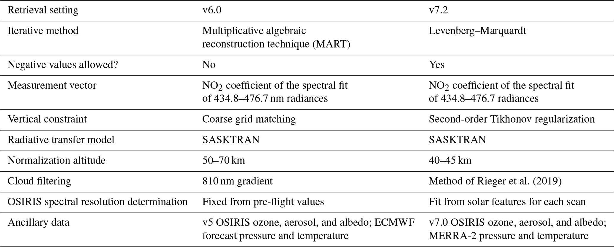
The zonal mean differences between v6.0 and v7.2 are shown in Fig. 2. The v7.2 NO2 concentrations are greater than those of v6.0 NO2, with the largest differences below 20 km. The observed differences are encouraging, suggesting that the observed low biases in v6.0 validation efforts will be reduced in v7.2. Later sections will explore this further, comparing both v6.0 and v7.2 to co-located satellite measurements.
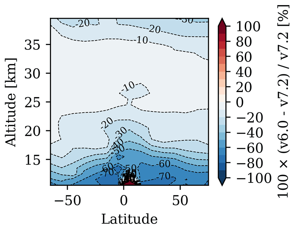
Figure 2Mean percent difference between v6.0 and v7.2 OSIRIS NO2 for all observations from November 2001 to May 2020. Bin spacing is 1 km and 10 degrees of latitude.
The second goal of v7.2 was to improve the response in the UTLS. Figure 3 shows the distributions of the v6.0 and v7.2 NO2 in 20∘ latitude bins for every third altitude level below 24.5 km. The v7.2 NO2 is normally distributed, but the v6.0 NO2 has a log-normal distribution shape at the lower altitudes. We expect the retrieved NO2 to be normally distributed because the distributions are dominated by the precision of the measurements rather than geophysical NO2 variation at the lowest altitudes. Thus log-normal distributions are less physically realistic and are likely a result of the low bias in the v6.0 retrieval, combined with the inability of the v6.0 retrieval to retrieve negative number density values.
2.5 Averaging-kernel-based lower bound
The limb scatter technique rapidly loses sensitivity to NO2 in the UTLS due to an increased optical path length and relatively low values of NO2. The combination of the averaging kernel and retrieval error covariance matrix characterizes this loss of sensitivity; however, for many scientific applications it is not possible to consider the averaging kernel directly in the analysis. For this reason a filter based on the averaging kernel for each profile was developed as a way to put a lower altitude limit on the retrieved NO2. The averaging kernel A relates the change in the retrieved atmospheric state, , to the change in the true state, x,
which characterizes the information content of the retrieval.
Ideally the averaging kernel is a sharply peaked Gaussian at the altitude for which we are retrieving information: the width of the averaging kernel defines the spatial resolution of the retrieval. This allows us to use the width of the averaging kernel and the altitude at which it peaks to characterize the performance of the retrieval.
Figure 4a shows the 15.5 and 30.5 km averaging kernels for a sample OSIRIS scan, with the Gaussian fits overlaid as dashed lines. The reported retrieval altitudes are marked with solid black lines and the peak altitudes of the Gaussian are marked with dashed black lines. The difference between these altitudes is calculated for each averaging kernel. By inspection of these differences it was determined that the filter should remove all measurements below the highest altitude at which the altitude difference is greater than or equal to 1.5 km. Several values were tested, and a threshold of 1.5 km provides a compromise between including information that is far from the tangent point, and removing what are likely real geophysical signals. Figure 4b, c, and d show the NO2 profile, FWHM, and altitude difference for a sample OSIRIS profile, respectively. While there is nothing obviously unusual about the NO2 itself, the FWHM increases below 15.5 km and the difference between the peak averaging kernel altitude and the reported retrieval altitude becomes greater than 1.5 km at 15.5 km. Therefore, in this case the kernel filter says that the retrieval is adding minimal information below 15.5 km, and thus the NO2 values at lower altitudes should not be used.
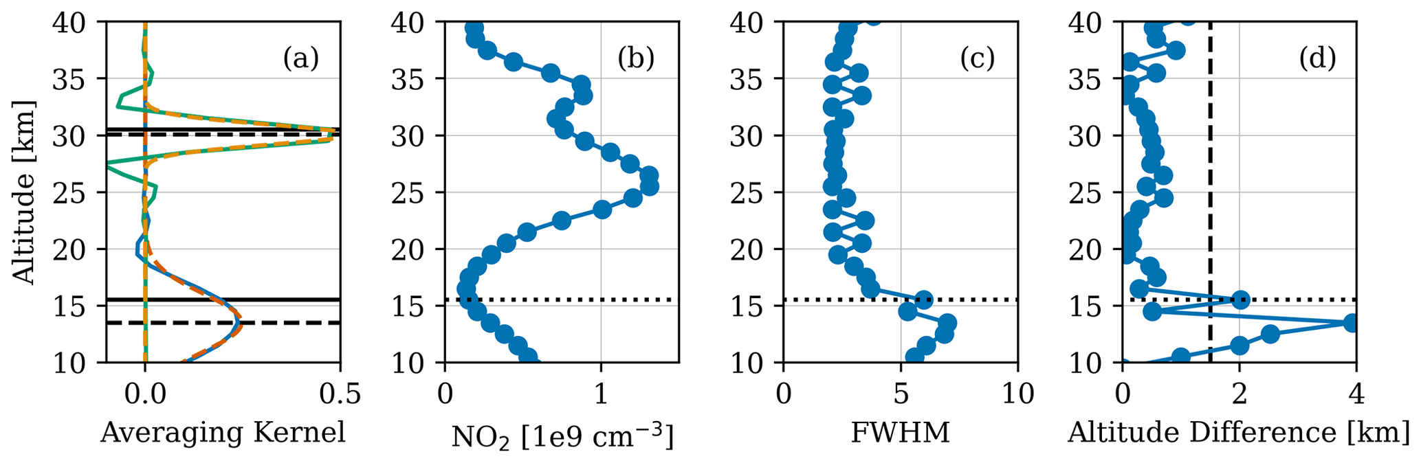
Figure 4NO2 retrieval diagnostics for OSIRIS scan 3292102 (8 March 2007, 23.9∘ N). (a) Averaging kernels at 15.5 km (blue) and 30.5 km (green). The dashed red line is the Gaussian fit to the 15.5 km averaging kernel and the dashed orange line is the Gaussian fit to the 30.5 km averaging kernel. The solid black lines mark the retrieval altitudes and the dashed black lines mark the peak altitude of the Gaussian fits. (b) NO2 profile. (c) FWHM of the averaging kernels. (d) Difference between averaging kernel altitude and reported retrieval altitude. The dashed black line marks a difference of 1.5 km. In the last three panels the dotted black line is the altitude at which the kernel filter would cut off this profile.
Figure 5a shows the percentage of NO2 data in 2010 at each altitude and latitude that is successfully retrieved, and that is above the cloud top (OSIRIS measures scattered sunlight so it is incapable of measuring anything below the cloud top). Up to 25 % of the data is retrieved down to 10 km, which is well into the troposphere in the tropics. The dashed orange line in Fig. 5 is the average tropopause height based on the temperature lapse rate (the value is provided with each OSIRIS profile). The solid orange line is the average 380 K potential temperature height. It was calculated using the temperature and pressure information included with the OSIRIS NO2 data. This level is an alternative definition of the tropopause location. Figure 5b shows the percentage of the data that remains after applying the averaging kernel filter to the v7.2 retrieved NO2. The majority of the NO2 data below the lapse rate tropopause is removed. Based on this filter, only about 20 % of the NO2 profiles extend down to ∼16 km in the tropics and ∼ 12 km at higher latitudes.

Figure 5(a) The percentage of data that are retrieved and above the cloud top. (b) The percentage of data that remain after applying the averaging kernel filter. The solid orange line is the average altitude of the 380 K potential temperature. The dashed orange line is the mean tropopause height based on the temperature lapse rate. The percentages were calculated for all OSIRIS profiles from 2010.
3.1 ACE-FTS
ACE-FTS has been in orbit on SCISAT since 2003 and collecting data since February 2004. It is in a high-inclination circular orbit (74∘) at 650 km. ACE-FTS is an infrared Fourier transform spectrometer, measuring from 750 to 4400 cm−1, with a resolution of 0.02 cm−1 (Boone et al., 2005, 2013). There are typically 30 occultation events each day, 15 at sunrise and 15 at sunset.
Vertical profiles for over 40 molecules and over 20 isotopologues are retrieved from the ACE-FTS measurements. The observed interferograms are first converted to atmospheric transmission spectra, and then the volume mixing ratio is retrieved from each spectrum using a non-linear least-squares technique (Boone et al., 2013). The v3.5 NO2 retrieval uses 40 microwindows between 1204.4 and 2950.9 cm−1, and the retrieved profiles extend from a minimum altitude of 7 km to a maximum altitude of 52 km. The retrieval uses global fitting, assumes horizontal homogeneity, and does not require a priori NO2 data (only a first guess). It also accounts for interfering species (e.g. H2O, CH4, OCS).
A detailed validation of the v3.5 NO2 retrieval is given in Sheese et al. (2016). Note that a change in the processor is the only difference between v3.5 and v3.6. The current recommended version is v4.2. The only difference between v4.1 and v4.2 is the global environment settings, which caused no significant difference between v4.1 and v4.2 NO2 volume mixing ratios; v4.1 is described in Boone et al. (2020). The changes from v3.6 to v4.1 and v4.2 had a minimal effect on the retrieved NO2: the difference between the two versions is within ± 5 % at most latitudes and altitudes above 15 km. Here we focus on v4.1 and v4.2.
3.2 SAGE III/ISS
SAGE III has been collecting data from the ISS since June 2017. The inclination of the ISS is 51.6∘, which allows SAGE III/ISS to view latitudes from 70∘ N to 70∘ S. It uses a configurable charge-coupled device (CCD) spectrometer, observing wavelengths from 280 to 1035 nm, with a 1–2 nm resolution. A separate photodiode observes from 1542 ± 15 nm. SAGE III/ISS continuously scans back and forth across the sun during each occultation in order to measure the irradiance as a function of altitude. There are typically 16 sunrise and 16 sunset events per day.
The measured irradiances are used to determine the O3, NO2, and H2O number densities, along with the aerosol extinction at several wavelengths. The algorithm first uses the measured irradiance to calculate slant path transmission profiles for each channel. Each slant path transmission profile is converted to a slant path optical depth profile containing contributions from Rayleigh scattering, aerosol extinction, and absorption by at least one species. Multiple linear regression is then used to solve for the NO2 and O3 slant path number density profiles simultaneously. NO2 is retrieved from channel S3 (433–450 nm). A global fit method is used to convert the slant path number density to vertical number density profiles. Further details on the retrieval are given in the SAGE III Algorithm Theoretical Basis Document (2002). The NO2 number density is available from 10 to 45 km on a 0.5 km grid with a vertical resolution of around 1.5 km. The reported uncertainty due to measurement noise in the SAGE III/ISS NO2 is approximately 5 % at 30 km, increasing up to 20 % at 10 and 40 km.
The recent v5.2 retrieval algorithm improves upon the v5.1 algorithm in many aspects, the most important being the refined wavelength map and bandpass for the spectrograph. Additional improvements relevant to NO2 include better oxygen dimer (O4) corrections and the removal of all vertical smoothing of the input Level 1 transmission profiles. In addition, the number density profiles are not smoothed in v5.2 as they were in v5.1. A five-point triangular smoothing was applied to each individual profile used here in order to better compare with v5.1. This smoothing is comparable to the 2–3 km vertical resolution provided by OSIRIS.
3.2.1 The diurnally varying retrieval
Photochemistry causes the NO2 number density to vary throughout the course of a day. During an occultation measurement the solar zenith angle (SZA) is 90∘ at the tangent point, but it varies along the line of sight (LOS). The SAGE III/ISS and ACE-FTS NO2 retrieval algorithms both neglect these deviations along the instrument's LOS by assuming there is a constant gradient in the NO2 number density with respect to the vertical dimension within each layer of the atmosphere. This assumption can result in retrieved NO2 that is biased high at the tangent point.
Dubé et al. (2021) describes an update to the SAGE III/ISS retrieval that accounts for variations in NO2 along the LOS (referred to as the diurnally varying (DV) retrieval). They used the NO2 number densities from the SAGE v5.1 retrieval. The NO2 values at each point along the LOS for a given scan were scaled to the SZA at that location using factors calculated with the PRATMO photochemical box model (Prather and Jaffe, 1990; McLinden et al., 2000). The input to PRATMO is an atmospheric state, consisting of pressure, temperature, air density, and O3 profiles. These values are set to be those provided with the SAGE III/ISS NO2 data. The sensitivity of the PRATMO NO2 to the exact values of the input parameters was estimated by perturbing them in the model. The effect on NO2 is small, with NO2 being most sensitive to changes in temperature: a variation on the order of −1∘ K results in a 1 % change in NO2. The PRATMO inputs are kept constant as the model iterates over a set of chemical reactions for a single day. This continues until the start and end values converge. The result is a 24 h steady-state system of each species in the model. This allows us to get the NO2 number density at any specified SZA.
Dubé et al. (2021) found that accounting for diurnal variations in the SAGE III/ISS retrieval improved agreement between SAGE III/ISS and OSIRIS NO2 by up to 20 % below 25 km. This DV retrieval, applied to both SAGE v5.1 and v5.2 NO2 products, is considered in the comparisons with OSIRIS presented here, along with the standard SAGE v5.1 and v5.2 retrievals.
The coincidence criteria are 1 d, 5∘ latitude, and 10∘ longitude. Figure 6 shows the number of coincident profiles with OSIRIS in each 10∘ latitude bin for both ACE-FTS and SAGE III/ISS. The ACE-FTS orbit results in significantly more coincidences at the high latitudes. The relatively low number of coincidences between OSIRIS and SAGE III/ISS is due to the much shorter overlap period between the missions, compared to OSIRIS and ACE-FTS. Most latitude bins still have at least 100 pairs. The lack of coincidences with SAGE III/ISS from 0 to 30∘ in the Northern Hemisphere is because OSIRIS took few measurements in this region during 2019 and 2020, which makes up the bulk of the overlap with the SAGE III/ISS mission.
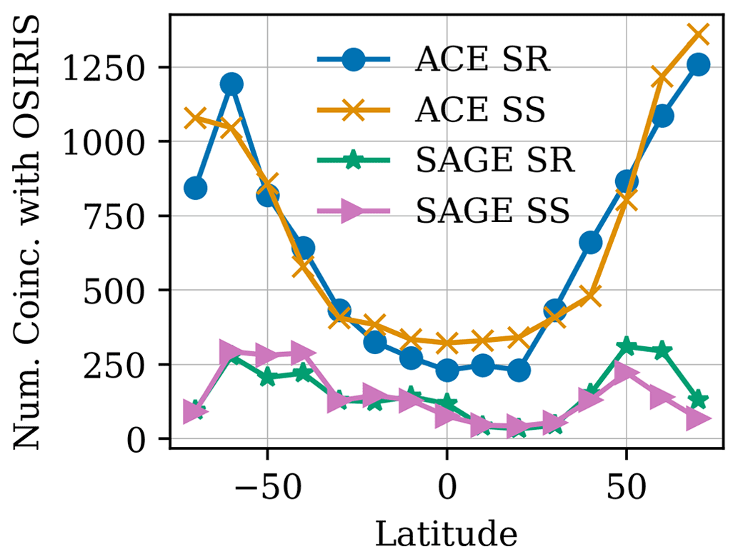
Figure 6Number of coincident profiles in each 10∘ latitude bin for ACE-FTS and SAGE III/ISS with OSIRIS at 25.5 km. SS refers to sunset occultations, while SR refers to sunrise occultations.
The daily photochemical cycle results in considerably different NO2 concentrations at sunrise and sunset (when ACE-FTS and SAGE III/ISS measure) and near 06:30 LST (when OSIRIS measures). This must be accounted for before the different datasets can be compared. All datasets were shifted to a common local solar time of 12:00 LST using PRATMO. The ratio of the model NO2 at 12:00 LST to the model NO2 at the instrument measurement time is used to scale the measured NO2 to 12:00 LST. This method is further described in Dubé et al. (2020).
While this scaling generally works well, it cannot always account for the differences between sunrise and sunset occultations from a single instrument. As an example, Fig. 7 compares the OSIRIS and ACE-FTS NO2 distributions at three altitudes in the tropics (left), at mid-latitudes (centre), and at high latitudes (right). The labels OSIRIS SR and OSIRIS SS refer to OSIRIS coincidences with ACE-FTS sunrise and sunset occultations, respectively. After scaling to 12:00 LST, the sunrise and sunset distributions in the tropics and mid-latitudes have similar shapes but a bias in the mean values. At high latitudes there is a clear double-peak structure in the ACE-FTS sunset measurements and corresponding OSIRIS coincident data. This shape is caused by the time of year at which the measurements are taken. The sunrise coincidences are mostly from the NH summer months, but the sunset coincidences also include NH spring observations. The sunrise distribution at these latitudes has a different shape than the sunset distribution. One should be cautious of this difference in shape and the bias between the mean values if intending to combine sunrise and sunset NO2 data from ACE-FTS (or SAGE III/ISS). In order to avoid any such complications we consider sunrise and sunset occultations separately throughout this work.
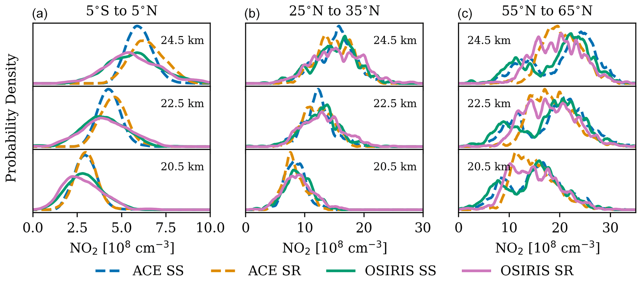
Figure 7Probability densities for ACE-FTS v4.1 and OSIRIS v7.2 coincident NO2, after shifting from their individual local times to 12:00 LST, for several altitudes from 5∘ S to 5∘ N (a) and from 55 to 65∘ N (c).
4.1 Comparison with ACE-FTS
As an example, Fig. 8 shows coincident ACE-FTS and OSIRIS NO2 profiles from 5 to 15∘ latitude. This bin is representative of the difference profile structure in the Northern Hemisphere. OSIRIS v7.2 shows better agreement with ACE-FTS than v6.0 above 20 km. As expected, there is minimal difference in the NO2 from the two ACE-FTS retrievals. The percent difference between OSIRIS and ACE-FTS is of comparable magnitude at both sunrise and sunset, except at the highest altitudes where OSIRIS v7.2 agrees better with the ACE sunset data. The cloud and averaging kernel filters result in OSIRIS v7.2 having fewer data points than v6.0 below ∼ 20 km, which could be why v6.0 shows better agreement with ACE-FTS at the lower altitudes.
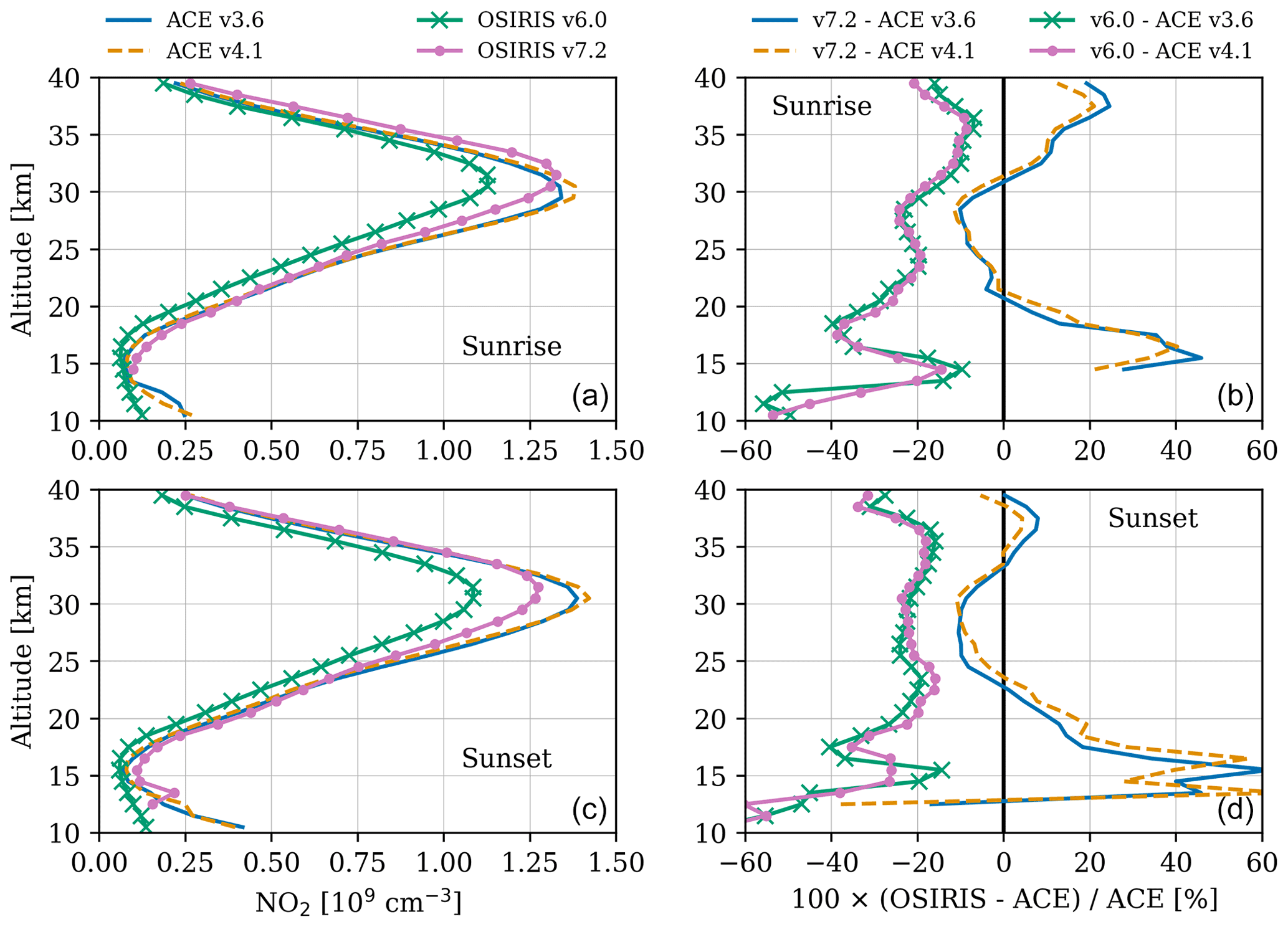
Figure 8Comparison of mean coincident ACE-FTS and OSIRIS NO2 profiles from 5 to 15∘ latitude. (a, b) ACE-FTS sunrise occultations. (c, d) ACE-FTS sunset occultations.
Figure 9 shows the mean percent difference between coincident ACE-FTS and OSIRIS NO2 profiles for several versions of the OSIRIS retrieval. This figure only considers the ACE-FTS v4.1 retrieval as the difference from the v3.6 retrieval is minimal. The first column compares OSIRIS v6.0 to ACE-FTS. OSIRIS is biased low everywhere, with the most negative bias occurring at lower altitudes. The middle column compares OSIRIS v7.2 to ACE-FTS. OSIRIS is lower than ACE-FTS in the Southern Hemisphere below 30 km and higher than ACE-FTS above 30 km. The lower bias in the Southern Hemisphere appears in the comparisons with both OSIRIS v6.0 and v7.2 NO2 so it is likely a feature of the ACE-FTS NO2 product. In the Northern Hemisphere the OSIRIS profiles coincident with ACE-FTS have a higher mean NO2 value than the profiles from the full OSIRIS mission.
For the most part the difference between ACE-FTS and OSIRIS v7.2 is less than the difference between ACE-FTS and OSIRIS v6.0. The only regions this is not true are for the sunrise measurements (top row) above 33 km and for both sunrise and sunset in the troposphere. Including the averaging kernel filter for the OSIRIS data reduces the bias with ACE-FTS sunset occultations in the troposphere by up to ∼ 50 % from the v7.2 difference without the filter.
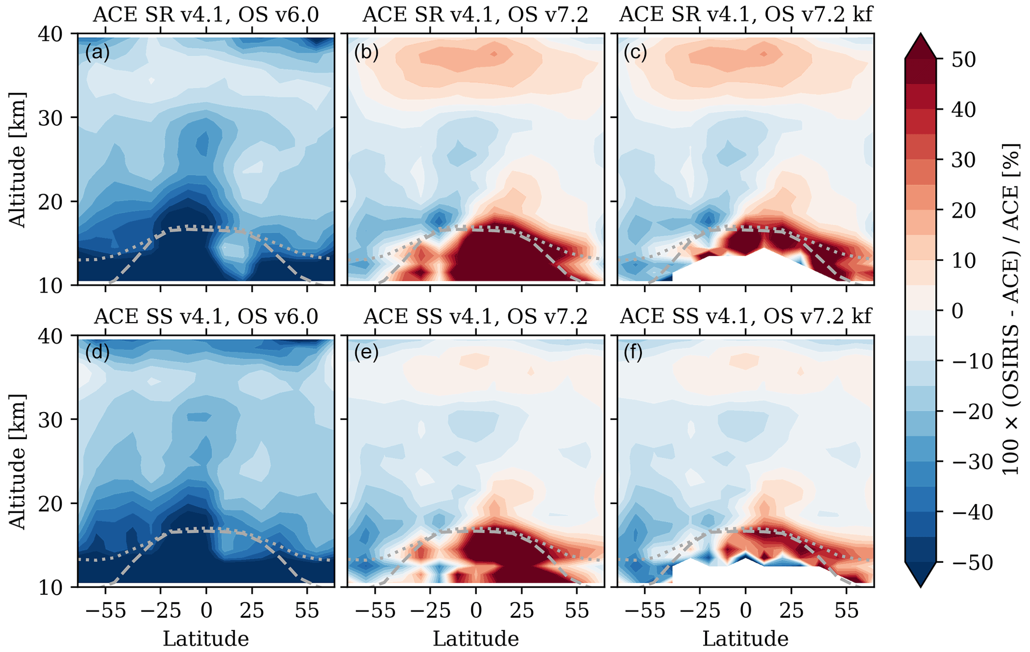
Figure 9Mean percent difference between coincident profiles from ACE-FTS v4.1 and OSIRIS. (a–c) Sunrise occultations. (d–f) Sunset occultations. The last column is the same as the centre column, but with the averaging kernel filter applied to the OSIRIS NO2. In all panels the dashed line is the average tropopause altitude and the dotted line is the average 380 K potential temperature altitude.
4.2 Comparison with SAGE III/ISS
Figure 10 compares coincident SAGE III/ISS and OSIRIS NO2 profiles from −25 to 15∘ latitude. This sample bin generally represents the differences between SAGE III/ISS and OSIRIS in the Southern Hemisphere. OSIRIS is biased lower than SAGE III/ISS at all altitudes for each retrieval version included in Fig. 10. The best agreement occurs between OSIRIS v7.2 and SAGE III/ISS DV v5.2 (the most recent version for each instrument). Including the diurnal correction reduces the SAGE III/ISS NO2 by about 10 % at 25 km and more than 10 % at lower altitudes (see Fig. 7 of Dubé et al., 2021). For the most part the magnitudes of the differences between OSIRIS v7.2 and SAGE III/ISS are comparable for both sunrise and sunset occultations.

Figure 10Comparison of mean coincident SAGE III/ISS and OSIRIS NO2 profiles from −25 to −15∘ latitude. (a, b) SAGE sunrise occultations. (c, d) SAGE III/ISS sunset occultations.
Figure 11 shows the mean percent difference between coincident SAGE III/ISS and OSIRIS NO2 profiles for the v5.2 diurnally varying SAGE III/ISS retrieval. The difference between SAGE III/ISS and OSIRIS is smaller for v7.2 of the OSIRIS retrieval than for v6.0 at all latitudes above 20 km. The agreement is better with sunrise (rather than sunset) occultations at the higher altitudes (which is the opposite of what we see when comparing to ACE). The averaging kernel filter removes some of the values with a very high difference at the low altitudes. For the sunset NO2 there is still a region remaining where OSIRIS is biased quite high. In this region the diurnally varying retrieval has a large effect, resulting in much lower SAGE III/ISS data. This increases the bias with OSIRIS compared to using the standard SAGE III/ISS retrieval (discussed in Dubé et al., 2021).

Figure 11Mean percent difference between coincident profiles from SAGE III/ISS and OSIRIS. (a–c) Sunrise occultations. (d–f) Sunset occultations. The last column is the same as the centre column but with the averaging kernel filter applied to the OSIRIS NO2. In all panels the dashed line is the average tropopause altitude, while the dotted line is the average 380 K potential temperature altitude.
4.3 The diurnal effect
Neither the OSIRIS retrieval nor the ACE-FTS retrieval accounts for diurnal variations in NO2 along the instrument's LOS. This effect can result in a significant bias in the data below ∼25 km. Here we estimate the effect of diurnal variations on the percent difference between NO2 from OSIRIS and ACE-FTS and OSIRIS and SAGE III/ISS. Note that the magnitude of the bias caused by neglecting the diurnal effect is expected to be the same in all versions of the OSIRIS and ACE-FTS NO2 data.
The magnitude of the diurnal effect depends on the direction of the LOS relative to the sun. For occultation instruments the SZA is always 90∘, but for limb scatter instruments the SZA is not consistent. McLinden et al. (2006) examined the effect of diurnal variations in retrievals of NO2 from OSIRIS and found that neglecting the diurnal effect can introduce a bias of 10 % to 35 % in the lower stratosphere for ∼16 % of the NO2 profiles. The bias is greater the closer the SZA is to 90∘. Based on the findings of McLinden et al. (2006) we repeated our analysis using only OSIRIS scans that have a SZA < 85∘. This reduced the number of coincidences with ACE-FTS by 14 % and the number of coincidences with SAGE III/ISS by 12 %. The majority of the removed coincidences were in the Southern Hemisphere. Figure 12 shows the change in the bias between OSIRIS and ACE-FTS and OSIRIS and SAGE III/ISS after excluding these coincident profiles. In Fig. 12 a negative number means that removing OSIRIS scans with a significant diurnal effect improved the agreement (reduced the bias). In general the only significant changes to the mean percent difference between ACE-FTS and OSIRIS NO2 occur below the tropopause. For SAGE III/ISS the difference is also small in most bins above the tropopause, although it does decrease by up to 10 % in some bins in the lower stratosphere. This bias with the SAGE III/ISS sunset occultations also decreases noticeably at all altitudes near −50∘, which is where the majority of the removed OSIRIS coincidences occur.
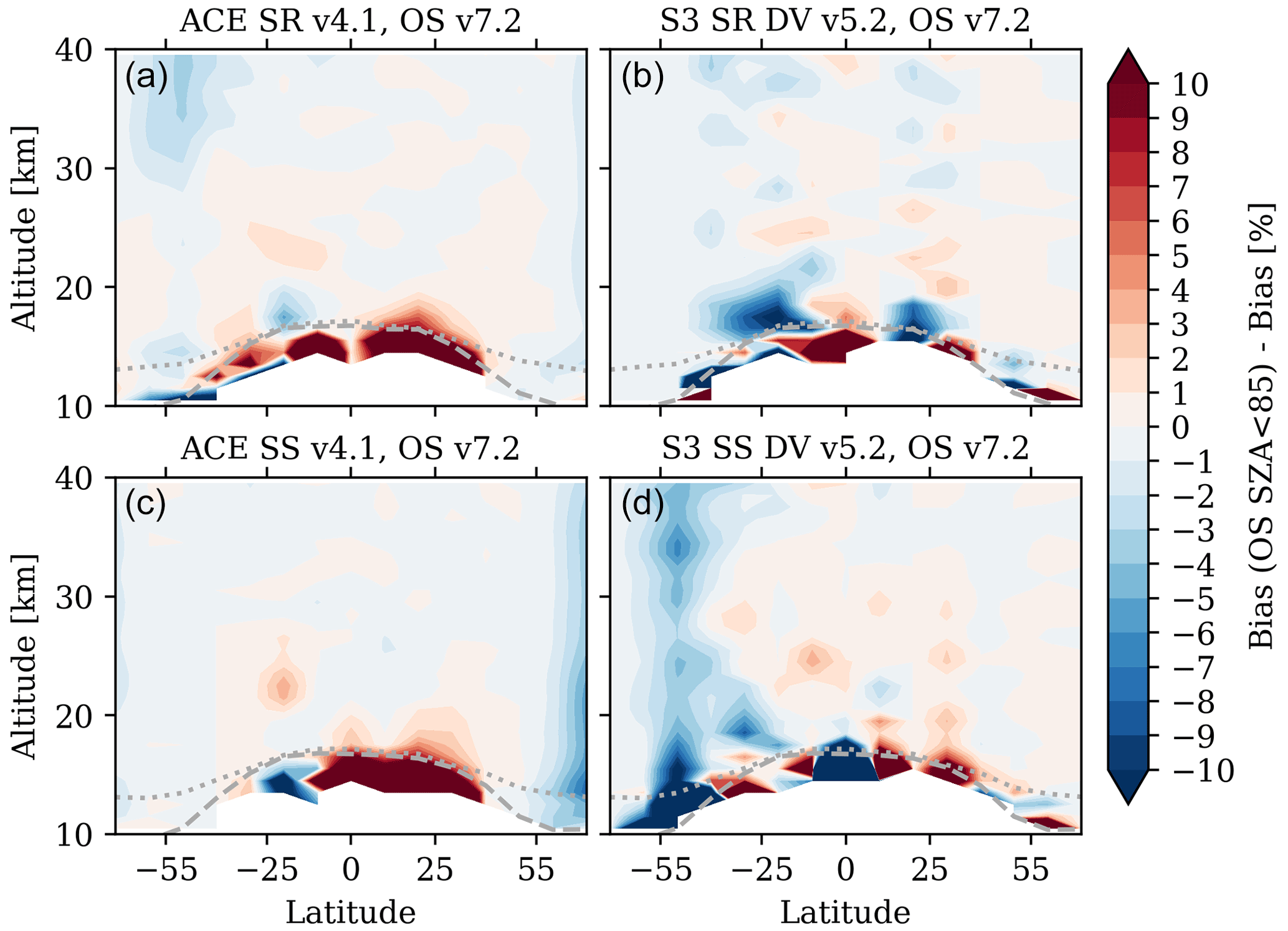
Figure 12Difference between the bias with and without including OSIRIS scans with SZA <85∘. (a) ACE-FTS sunrise occultations. (b) SAGE III/ISS sunrise occultations. (c) ACE-FTS sunset occultations. (d) SAGE III/ISS sunset occultations. In all panels the dashed line is the average tropopause altitude, while the dotted line is the average 380 K potential temperature altitude.
It is also necessary to consider the effect of diurnal variations in the ACE-FTS NO2. Based on the results of Dubé et al. (2021) for SAGE III/ISS and of Brohede et al. (2007) for a simulated occultation instrument, we expect there to be a high bias of greater than 10 % in the ACE NO2 below ∼30 km. Accounting for this effect would improve the agreement with OSIRIS in the SH but decrease agreement in the NH where ACE is already low compared to OSIRIS.
4.4 Time series comparison
Figure 13 shows the monthly mean relative anomaly time series for OSIRIS v7.2, SAGE III/ISS v5.2 DV, and ACE-FTS v4.1 NO2 in several bins. The relative anomaly is calculated by subtracting the overall mean value for a given month from all values for that month to remove the seasonal cycle (e.g. the mean June NO2 concentration is subtracted from each individual June NO2 concentration) and then dividing by the overall mean of the data. The relative anomaly allows for sources of variability (apart from the seasonal cycle) to be more easily detected. The bins were chosen to show a range of latitudes and altitudes, with a focus on the lower altitudes as this is where OSIRIS v7.2 NO2 changed most from the previous version. The anomaly time series for several more bins are provided in Appendix A. Overall, the datasets shows similar variability over a range of altitudes and latitudes. The correlation of OSIRIS with ACE-FTS sunset NO2 is greater than 0.7 at most latitudes from 20 to 35 km, and the correlation with ACE-FTS sunrise NO2 is greater than 0.5 at most latitudes. The correlation of OSIRIS with SAGE III/ISS is slightly lower but still greater than 0.5 at most altitudes above 20 km from −40 to 40∘. The lower correlation is likely because there are only a few years of SAGE III/ISS data available.
The ACE-FTS sunrise NO2 is noisier than the sunset data in the top panel of Fig. 13 (low altitude and high latitude). Sheese et al. (2016) suggested that this is because of differences in the diurnal variation along the LOS between sunrise and sunset observations. At sunrise ACE-FTS samples a region of the atmosphere that has not been illuminated long enough for the NO2 to reach equilibrium; however, this is not an issue at sunset. If this was indeed the problem it should also affect the SAGE III/ISS sunrise NO2 but that is not the case. In addition, the SAGE III/ISS anomaly time series looks very similar, whether or not the diurnal variations along the LOS are included in the retrieval.
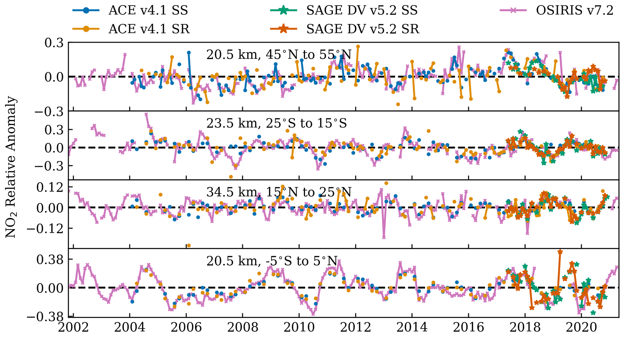
Figure 13Anomaly time series comparing OSIRIS v7.2 to ACE v4.1 and SAGE III/ISS v5.2 DV for four latitude/altitude bins.
There is significant variability within each panel of Fig. 13. Dubé et al. (2020) merged the previous OSIRIS v6.0 NO2 with NO2 from SAGE II and found that elevated aerosol levels and the quasi-biennial oscillation were the main factors influencing the NO2 anomaly. Dubé et al. (2020) also showed that there is a significant increasing trend in NO2 of 8 %–10 % in the tropical lower stratosphere from 1984 to 2014.
A new version of the OSIRIS NO2 retrieval was developed with the goal of reducing an observed low bias in the previous OSIRIS NO2 version and improving the retrieval response in the UTLS. The major improvements are better knowledge of the OSIRIS spectral resolution, attempts to reduce the effect of residual stray light, a different iterative scheme to improve convergence, and better cloud filtering. The improved spectral fitting and the lowering of the normalization altitude to reduce stray light are the main factors that result in higher retrieved NO2 number densities. A filter based on the averaging kernel was also developed as a way to determine the lowest altitude at which the retrieved NO2 contains useful information. The values for this filter are provided in the OSIRIS v7.2 data files. This new OSIRIS v7.2 NO2 retrieval was compared to coincident profiles from two occultation instruments: ACE-FTS and SAGE III/ISS. PRATMO was used to scale all datasets to 12:00 LT to account for the diurnal cycle in NO2 before performing the comparisons. OSIRIS v7.2 agrees better with NO2 from both ACE-FTS and SAGE III/ISS than the previous OSIRIS v6.0. The agreement is within 20 % at most latitudes and altitudes. In general OSIRIS agrees better with ACE-FTS than with SAGE III/ISS, although this could be due to the higher number of coincidences with ACE-FTS.
OSIRIS agrees slightly better with ACE-FTS sunset (rather than sunrise) occultations. The bias between OSIRIS v7.2 and ACE-FTS sunset is within 10 % above 20 km. This is likely because the ACE-FTS sunrise data is noisier. Conversely, OSIRIS agrees slightly better with SAGE III/ISS sunrise occultations (rather than sunset). The average sunset profile has a higher peak NO2 number density than the average sunrise profile, resulting in a greater bias with OSIRIS. As noted, the photochemical scaling to 12:00 LST is not able to account for all the differences between measurements taken at sunrise and sunset, when there are considerable changes occurring in the nitrogen chemistry.
NO2 from the SAGE III/ISS DV retrieval shows improved agreement with OSIRIS compared to NO2 from the standard SAGE retrieval. The diurnal effect produces a high bias in NO2 retrieved from occultation instruments below 25 km. There is no version of the ACE-FTS NO2 retrieval that accounts for diurnal variations along the line of sight, which could be increasing the difference with OSIRIS below about 25 km. It is not expected that the diurnal effect would be greater in ACE-FTS than in SAGE III/ISS, so this will add at most a 5 % to 40 % bias, with the largest bias at the lowest altitudes (Dubé et al., 2021). If we assume an approximate high bias of 25 % below 20 km in the ACE-FTS NO2, the difference between ACE-FTS and OSIRIS will become greater near the tropopause and especially in the NH. The bias in this region will be >50 %, as it is for SAGE III/ISS and OSIRIS. In the SH the bias between ACE-FTS and OSIRIS is % below 20 km. In this region, including the diurnal correction will result in a bias of ∼10 %, corresponding to improved agreement between OSIRIS and ACE-FTS. This is opposite in sign and smaller in absolute value than the bias between SAGE III/ISS and OSIRIS in this region. There are significantly more coincidences between ACE-FTS and OSIRIS than there are between SAGE III/ISS and OSIRIS at Southern Hemisphere mid-latitudes and high latitudes, which could explain why we see a smaller bias between ACE-FTS and OSIRIS.
We also considered the effect of diurnal variations along the OSIRIS LOS by repeating the analysis using only OSIRIS scans with a SZA < 85∘, corresponding to scans shown by McLinden et al. (2006) to have a significant bias. Removing these scans had a minimal effect on the comparisons between OSIRIS and ACE-FTS in the stratosphere, changing the bias by at most 3 %. It had a greater effect on the comparison with SAGE III/ISS, where the agreement improved by up to 10 % in some bins in the lower stratosphere.
The anomaly time series from each dataset shows very similar variability. Both ACE-FTS and OSIRIS are ageing, and thus it will soon be necessary to use a newer instrument like SAGE III/ISS to extend the NO2 data record. The good agreement between the time series provides confidence that SAGE III/ISS NO2 can easily be combined with NO2 from OSIRIS and/or ACE-FTS in the same manner that Dubé et al. (2020) combined NO2 from SAGE II (the precursor to SAGE III/ISS) and OSIRIS. These long-term datasets are important for monitoring the trend in NO2 as increasing anthropogenic N2O emissions and the associated increase in stratospheric NO2 can result in a decrease of O3.
Overall, we conclude based on comparison with NO2 from ACE-FTS and SAGE III/ISS that the OSIRIS v7.2 NO2 product is an improvement over the previous v6.0 OSIRIS NO2, particularly below 30 km. The bias between OSIRIS v7.2 and both ACE-FTS and SAGE III/ISS has decreased from v6.0, except for in a few bins near the tropopause where including the diurnal effect in SAGE III/ISS (or estimating the magnitude of the effect for ACE-FTS) makes the bias greater than it was in v6.0
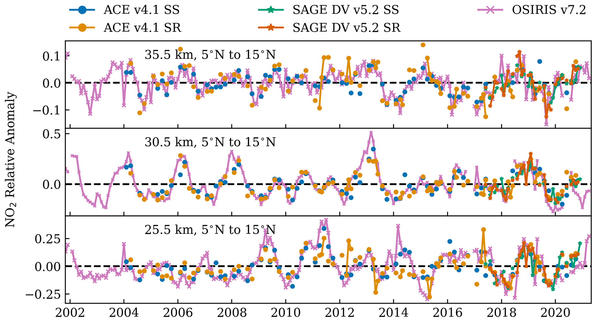
Figure A1Anomaly time series comparing OSIRIS v7.2 to ACE v4.1 and SAGE III/ISS v5.2 DV for three altitudes in the tropics.
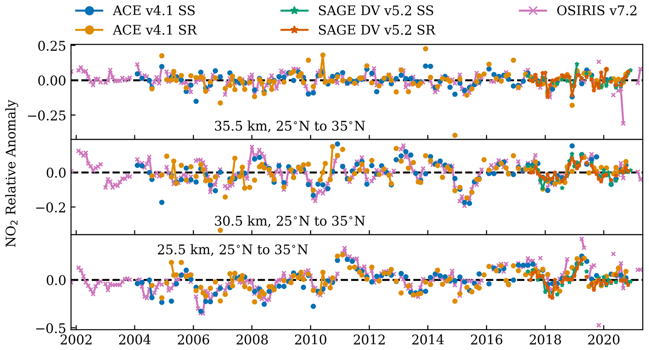
Figure A2Anomaly time series comparing OSIRIS v7.2 to ACE v4.1 and SAGE III/ISS v5.2 DV for three altitudes at Northern Hemisphere subtropics.

Figure A3Anomaly time series comparing OSIRIS v7.2 to ACE v4.1 and SAGE III/ISS v5.2 DV for three altitudes at Northern Hemisphere mid-latitudes.
OSIRIS data are available at https://research-groups.usask.ca/osiris/data-products.php#OSIRISLevel2DataProducts (last access: 13 March 2022, Zawada et al., 2022). SAGE III/ISS data are available at https://asdc.larc.nasa.gov/project/SAGE III-ISS/g3bssp_52 (last access: 13 March 2022, NASA/LARC/SD/ASDC, 2017). SAGE III/ISS NO2 data corrected for diurnal variations are available at https://research-groups.usask.ca/osiris/data-products.php/#SAGEIII (last access: 13 March 2022, Dubé, 2022). ACE data are available at https://databace.scisat.ca/level2/ (last access: 13 March 2022, ACE-FTS, 2022). The PRATMO python package can be downloaded from https://arg.usask.ca/wheels/ (last access: 22 August 2022, University of Saskatchewan Atmospheric Research Group, 2022a), and the documentation is available at https://arg.usask.ca/docs/Pratmo/pratmo_boxmodel.html (last access: 22 August 2022, University of Saskatchewan Atmospheric Research Group, 2022b).
KD performed the analysis and prepared the manuscript. DZ created the OSIRIS v7.2 NO2 retrieval. AB and DD assisted with the analysis and the creation of the OSIRIS data. DF provided guidance on using the SAGE III/ISS data. PS provided guidance on using the ACE-FTS data. All authors provided significant feedback on the analysis and the manuscript.
The contact author has declared that none of the authors has any competing interests.
Publisher's note: Copernicus Publications remains neutral with regard to jurisdictional claims in published maps and institutional affiliations.
The authors thank the Swedish National Space Agency and the Canadian Space Agency for the continued operation and support of Odin-OSIRIS. The Atmospheric Chemistry Experiment (ACE) is a Canadian-led mission mainly supported by the CSA and the NSERC, and Peter Bernath is the principal investigator.
The OSIRIS mission is supported by the Canadian Space Agency (grant no. RGPIN 04850-2019). Kimberlee Dubé, Adam Bourassa, and Doug Degenstein were supported by NSERC (grant no. RGPIN 04850-2019).
This paper was edited by Folkert Boersma and reviewed by Chris McLinden and one anonymous referee.
Adams, C., Bourassa, A. E., McLinden, C. A., Sioris, C. E., von Clarmann, T., Funke, B., Rieger, L. A., and Degenstein, D. A.: Effect of volcanic aerosol on stratospheric NO2 and N2O5 from 2002–2014 as measured by Odin-OSIRIS and Envisat-MIPAS, Atmos. Chem. Phys., 17, 8063–8080, https://doi.org/10.5194/acp-17-8063-2017, 2017. a
ACE-FTS: Level 2 Data, Version 4.1/4.2, ACE-SCISAT Database [data set], https://databace.scisat.ca/level2/, last access: 13 March 2022. a
Bernath, P. F., McElroy, C. T., Abrams, M. C., Boone, C. D., Butler, M., Camy-Peyret, C., Carleer, M., Clerbaux, C., Coheur, P.-F., Colin, R., DeCola, P., DeMazière, M., Drummond, J. R., Dufour, D., Evans, W. F. J., Fast, H., Fussen, D., Gilbert, K., Jennings, D. E., Llewellyn, E. J., Lowe, R. P., Mahieu, E., McConnell, J. C., McHugh, M., McLeod, S. D., Michaud, R., Midwinter, C., Nassar, R., Nichitiu, F., Nowlan, C., Rinsland, C. P., Rochon, Y. J., Rowlands, N., Semeniuk, K., Simon, P., Skelton, R., Sloan, J. J., Soucy, M.-A., Strong, K., Tremblay, P., Turnbull, D., Walker, K. A., Walkty, I., Wardle, D. A., Wehrle, V., Zander, R., and Zou, J.: Atmospheric Chemistry Experiment (ACE): Mission overview, Geophys. Res. Lett., 32, L15S01, https://doi.org/10.1029/2005GL022386, 2005. a
Bognar, K., Zhao, X., Strong, K., Boone, C., Bourassa, A., Degenstein, D., Drummond, J., Duff, A., Goutail, F., Griffin, D., Jeffery, P., Lutsch, E., Manney, G., McElroy, C., McLinden, C., Millán, L., Pazmino, A., Sioris, C., Walker, K., and Zou, J.: Updated validation of ACE and OSIRIS ozone and NO2 measurements in the Arctic using ground-based instruments at Eureka, Canada, J. Quant. Spectrosc. Ra. Transf., 238, 106571, https://doi.org/10.1016/j.jqsrt.2019.07.014, 2019. a
Bognar, K., Tegtmeier, S., Bourassa, A., Roth, C., Warnock, T., Zawada, D., and Degenstein, D.: Stratospheric ozone trends for 1984–2021 in the SAGE II–OSIRIS–SAGE III/ISS composite dataset, Atmos. Chem. Phys., 22, 9553–9569, https://doi.org/10.5194/acp-22-9553-2022, 2022. a
Boone, C., Bernath, P., Cok, D., Jones, S., and Steffen, J.: Version 4 retrievals for the atmospheric chemistry experiment Fourier transform spectrometer (ACE-FTS) and imagers, J. Quant. Spectrosc. Ra. Transf., 247, 106939, https://doi.org/10.1016/j.jqsrt.2020.106939, 2020. a
Boone, C. D., Nassar, R., Walker, K. A., Rochon, Y., McLeod, S. D., Rinsland, C. P., and Bernath, P. F.: Retrievals for the atmospheric chemistry experiment Fourier-transform spectrometer, Appl. Opt., 44, 7218–7231, https://doi.org/10.1364/AO.44.007218, 2005. a
Boone, C. D., Walker, K. A., and Bernath, P. F.: Version 3 retrievals for the atmospheric chemistry experiment Fourier transform spectrometer (ACE-FTS), in: The Atmospheric Chemistry Experiment ACE at 10: a Solar Occultation Anthology, edited by: Bernath, P., vol. 10, 103–127, A. Deepak Publishing, 2013. a, b
Bourassa, A. E., Degenstein, D. A., and Llewellyn, E. J.: SASKTRAN: A spherical geometry radiative transfer code for efficient estimation of limb scattered sunlight, J. Quant. Spectrosc. Ra. Transf., 109, 52–73, https://doi.org/10.1016/j.jqsrt.2007.07.007, 2008. a
Bourassa, A. E., McLinden, C. A., Sioris, C. E., Brohede, S., Bathgate, A. F., Llewellyn, E. J., and Degenstein, D. A.: Fast NO2 retrievals from Odin-OSIRIS limb scatter measurements, Atmos. Meas. Tech., 4, 965–972, https://doi.org/10.5194/amt-4-965-2011, 2011. a
Brion, J., Chakir, A., Daumont, D., Malicet, J., and Parisse, C.: High-resolution laboratory absorption cross section of O3. Temperature effect, Chem. Phys. Lett., 213, 610–612, https://doi.org/10.1016/0009-2614(93)89169-I, 1993. a
Brohede, S. M., Haley, C. S., Mclinden, C. A., Sioris, C. E., Murtagh, D. P., Petelina, S. V., Llewellyn, E. J., Bazureau, A., Goutail, F., Randall, C. E., Lumpe, J. D., Taha, G., Thomasson, L. W., and Gordley, L. L.: Validation of Odin/OSIRIS stratospheric NO2 profiles, J. Geophys. Res.-Atmos., 112, D07310, https://doi.org/10.1029/2006JD007586, 2007. a, b, c
Cisewski, M., Zawodny, J., Gasbarre, J., Eckman, R., Topiwala, N., Rodriguez-Alvarez, O., Cheek, D., and Hall, S.: The Stratospheric Aerosol and Gas Experiment (SAGE III) on the International Space Station (ISS) Mission, in: Sensors, Systems, and Next-Generation Satellites XVIII, vol. 9241, p. 924107, International Society for Optics and Photonics, https://doi.org/10.1117/12.2073131, 2014. a
Dubé, K.: SAGE III/ISS NO2 profiles retrieved by accounting for diurnal variations, University of Saskatchewan Atmospheric Research Group [data set], https://research-groups.usask.ca/osiris/data-products.php/#SAGEIII, last access: 13 March 2022. a
Daumont, D., Brion, J., Charbonnier, J., and Malicet, J.: Ozone UV spectroscopy I: Absorption cross-sections at room temperature, J. Atmos. Chem., 15, 145–155, https://doi.org/10.1007/BF00053756, 1992. a
Dubé, K., Randel, W., Bourassa, A., Zawada, D., McLinden, C., and Degenstein, D.: Trends and Variability in Stratospheric NOx Derived From Merged SAGE II and OSIRIS Satellite Observations, J. Geophys. Res.-Atmos., 125, e2019JD031798, https://doi.org/10.1029/2019JD031798, 2020. a, b, c, d
Dubé, K., Bourassa, A., Zawada, D., Degenstein, D., Damadeo, R., Flittner, D., and Randel, W.: Accounting for the photochemical variation in stratospheric NO2 in the SAGE III/ISS solar occultation retrieval, Atmos. Meas. Tech., 14, 557–566, https://doi.org/10.5194/amt-14-557-2021, 2021. a, b, c, d, e, f
Haley, C. S. and Brohede, S.: Status of the Odin/OSIRIS stratospheric O3 and NO2 data products, Can. J. Phys., 85, 1177–1194, https://doi.org/10.1139/p07-114, 2007. a
Haley, C. S., Brohede, S. M., Sioris, C. E., Griffioen, E., Murtagh, D. P., McDade, I. C., Eriksson, P., Llewellyn, E. J., Bazureau, A., and Goutail, F.: Retrieval of stratospheric O3 and NO2 profiles from Odin Optical Spectrograph and Infrared Imager System (OSIRIS) limb-scattered sunlight measurements, J. Geophys. Res.-Atmos., 109, D16303, https://doi.org/10.1029/2004JD004588, 2004. a
Llewellyn, E. J., Lloyd, N. D., Degenstein, D. A., Gattinger, R. L., Petelina, S. V., Bourassa, A. E., Wiensz, J. T., Ivanov, E. V., McDade, I. C., Solheim, B. H., McConnell, J. C., Haley, C. S., von Savigny, C., Sioris, C. E., McLinden, C. A., Griffioen, E., Kaminski, J., Evans, W. F., Puckrin, E., Strong, K., Wehrle, V., Hum, R. H., Kendall, D. J., Matsushita, J., Murtagh, D. P., Brohede, S., Stegman, J., Witt, G., Barnes, G., Payne, W. F., Piché, L., Smith, K., Warshaw, G., Deslauniers, D. L., Marchand, P., Richardson, E. H., King, R. A., Wevers, I., McCreath, W., Kyrölä, E., Oikarinen, L., Leppelmeier, G. W., Auvinen, H., Mégie, G., Hauchecorne, A., Lefèvre, F., de La Nöe, J., Ricaud, P., Frisk, U., Sjoberg, F., von Schéele, F., and Nordh, L.: The OSIRIS instrument on the Odin spacecraft, Can. J. Phys., 82, 411–422, https://doi.org/10.1139/p04-005, 2004. a, b
Malicet, J., Daumont, D., Charbonnier, J., Parisse, C., Chakir, A., and Brion, J.: Ozone UV spectroscopy. II. Absorption cross-sections and temperature dependence, J. Atmos. Chem., 21, 263–273, https://doi.org/10.1007/BF00696758, 1995. a
McLinden, C. A., Olsen, S. C., Hannegan, B., Wild, O., Prather, M. J., and Sundet, J.: Stratospheric ozone in 3-D models: A simple chemistry and the cross-tropopause flux, J. Geophys. Res.-Atmos., 105, 14653–14665, https://doi.org/10.1029/2000JD900124, 2000. a, b
McLinden, C. A., Haley, C. S., and Sioris, C. E.: Diurnal effects in limb scatter observations, J. Geophys. Res.-Atmos., 111, D14302, https://doi.org/10.1029/2005JD006628, 2006. a, b, c
Murtagh, D., Frisk, U., Merino, F., Ridal, M., Jonsson, A., Stegman, J., Witt, G., Eriksson, P., Jiménez, C., Megie, G., Noë, J. d. l., Ricaud, P., Baron, P., Pardo, J. R., Hauchcorne, A., Llewellyn, E. J., Degenstein, D. A., Gattinger, R. L., Lloyd, N. D., Evans, W. F., McDade, I. C., Haley, C. S., Sioris, C., Savigny, C. v., Solheim, B. H., McConnell, J. C., Strong, K., Richardson, E. H., Leppelmeier, G. W., Kyrölä, E., Auvinen, H., and Oikarinen, L.: An overview of the Odin atmospheric mission, Can. J. Phys., 80, 309–319, https://doi.org/10.1139/p01-157, 2002. a
NASA/LARC/SD/ASDC: SAGE III/ISS L2 Solar Event Species Profiles (HDF5) V052, NASA Langley Atmospheric Science Data Center DAAC [data set], https://asdc.larc.nasa.gov/project/SAGE III-ISS/g3bssp_52 (last access: 13 March 2022), 2017. a
Prather, M. and Jaffe, A. H.: Global impact of the Antarctic ozone hole: Chemical propagation, J. Geophys. Res.-Atmos., 95, 3473–3492, https://doi.org/10.1029/JD095iD04p03473, 1990. a, b, c
Rieger, L. A., Zawada, D. J., Bourassa, A. E., and Degenstein, D. A.: A Multiwavelength Retrieval Approach for Improved OSIRIS Aerosol Extinction Retrievals, J. Geophys. Res.-Atmos., 124, 7286–7307, https://doi.org/10.1029/2018JD029897, 2019. a, b, c
SAGE III Algorithm Theoretical Basis Document, T.: SAGE III Algorithm Theoretical Basis Document (ATBD) Solar and Lunar Algorithm, Tech. rep., LaRC 475-00-109, https://eospso.gsfc.nasa.gov/sites/default/files/atbd/atbd-sage-solar-lunar.pdf (last access: 19 January 2021), 2002. a
Sheese, P. E., Walker, K. A., Boone, C. D., McLinden, C. A., Bernath, P. F., Bourassa, A. E., Burrows, J. P., Degenstein, D. A., Funke, B., Fussen, D., Manney, G. L., McElroy, C. T., Murtagh, D., Randall, C. E., Raspollini, P., Rozanov, A., Russell III, J. M., Suzuki, M., Shiotani, M., Urban, J., von Clarmann, T., and Zawodny, J. M.: Validation of ACE-FTS version 3.5 NOy species profiles using correlative satellite measurements, Atmos. Meas. Tech., 9, 5781–5810, https://doi.org/10.5194/amt-9-5781-2016, 2016. a, b, c
Sioris, C. E., Haley, C. S., McLinden, C. A., von Savigny, C., McDade, I. C., McConnell, J. C., Evans, W. F. J., Lloyd, N. D., Llewellyn, E. J., Chance, K. V., Kurosu, T. P., Murtagh, D., Frisk, U., Pfeilsticker, K., Bösch, H., Weidner, F., Strong, K., Stegman, J., and Mégie, G.: Stratospheric profiles of nitrogen dioxide observed by Optical Spectrograph and Infrared Imager System on the Odin satellite, J. Geophys. Res.-Atmos., 108, 4215, https://doi.org/10.1029/2002JD002672, 2003. a
Sioris, C. E., Rieger, L. A., Lloyd, N. D., Bourassa, A. E., Roth, C. Z., Degenstein, D. A., Camy-Peyret, C., Pfeilsticker, K., Berthet, G., Catoire, V., Goutail, F., Pommereau, J.-P., and McLinden, C. A.: Improved OSIRIS NO2 retrieval algorithm: description and validation, Atmos. Meas. Tech., 10, 1155–1168, https://doi.org/10.5194/amt-10-1155-2017, 2017. a, b, c
University of Saskatchewan Atmospheric Research Group: Software wheels, University of Saskatchewan [code], https://arg.usask.ca/wheels, last access: 22 August 2022a. a
University of Saskatchewan Atmospheric Research Group: Pratmo_BoxModel – pratmo 2.0 documentation, University of Saskatchewan [code], https://arg.usask.ca/docs/Pratmo/pratmo_boxmodel.html, last access: 22 August 2022b. a
Vandaele, A. C., Hermans, C., Simon, P. C., Carleer, M., Colin, R., Fally, S., Merienne, M.-F., Jenouvrier, A., and Coquart, B.: Measurements of the NO2 absorption cross-section from 42 000 cm−1 to 10 000 cm−1 (238–1000 nm) at 220 K and 294 K, J. Quant. Spectrosc. Ra. Transf., 59, 171–184, https://doi.org/10.1016/S0022-4073(97)00168-4, 1998. a
Zawada, D., Warnock, T., Bourassa, A., and Degenstein, D.: OSIRIS Level 2 Data: Version 7.2 NO2, University of Saskatchewan Atmospheric Research Group [data set], https://research-groups.usask.ca/osiris/data-products.php/#OSIRISLevel2DataProducts, last access: 13 March 2022. a
Zawada, D. J., Dueck, S. R., Rieger, L. A., Bourassa, A. E., Lloyd, N. D., and Degenstein, D. A.: High-resolution and Monte Carlo additions to the SASKTRAN radiative transfer model, Atmos. Meas. Tech., 8, 2609–2623, https://doi.org/10.5194/amt-8-2609-2015, 2015. a