the Creative Commons Attribution 4.0 License.
the Creative Commons Attribution 4.0 License.
 | 26 Oct 2022
Improved spectral processing for a multi-mode pulse compression Ka–Ku-band cloud radar system
Liping Liu
Cloud radars are widely used in observing clouds and precipitation. However, the raw data products of cloud radars are usually affected by multiple factors, which may lead to misinterpretation of cloud and precipitation processes. In this study, we present a Doppler-spectra-based data processing framework to improve the data quality of a multi-mode pulse-compressed Ka–Ku radar system. Firstly, non-meteorological signal close to the ground was identified with enhanced Doppler spectral ratios between different observing modes. Then, for the Doppler spectrum affected by the range sidelobe due to the implementation of the pulse compression technique, the characteristics of the probability density distribution of the spectral power were used to identify the sidelobe artifacts. Finally, the Doppler spectra observations from different modes were merged via the shift-then-average approach. The new radar moment products were generated based on the merged Doppler spectrum data. The presented spectral processing framework was applied to radar observations of a stratiform precipitation event, and the quantitative evaluation shows good performance of clutter or sidelobe suppression and spectral merging.
- Article
(8983 KB) - Full-text XML
- BibTeX
- EndNote


Clouds and precipitation are important for the Earth's energy budget and the hydrological cycle. Over the past few decades, a great deal of effort has been made to understand the microphysics and dynamics of clouds and precipitation. As remote sensing instruments, cloud radars operating in millimeter wavelengths have shown their unique role in addressing the observational gaps in clouds and precipitation (Kollias et al., 2002; Stephens et al., 2002; Illingworth et al., 2007; Li and Moisseev, 2020). Compared with weather radars, shorter wavelengths of cloud radars allow for the detection of small hydrometeors without the use of high-power transmitters and large antennas. Meanwhile, their compact size enables good portability, making them a powerful tool for observing clouds and weak precipitation (Kollias et al., 2007).
Most cloud radars work at the vertically pointing mode, and it is a common practice to use time–height plots to present the traditional radar data, such as equivalent reflectivity factor (Ze), mean Doppler velocity (V), and spectrum width (σ). These data products are also known as the moments of radar the Doppler spectrum, which is the decomposition of the radar return as a function of Doppler velocities (Kollias et al., 2011a). Radar Doppler spectra observations have been used to retrieve the dynamics (Shupe et al., 2008; Li et al., 2021; e.g., Zhu et al., 2021) and microphysics (Luke and Kollias, 2013; Tridon et al., 2013; Verlinde et al., 2013; Kalesse et al., 2016; e.g., Kneifel et al., 2016) of clouds and precipitation. However, preprocessing of radar Doppler spectra observations can be challenging due to the following issues.
(1) The contamination of non-meteorological signals. The non-meteorological echoes produced by stationary targets (e.g., buildings, trees, or terrain) and moving targets (e.g., insects, birds, or power lines moving in the wind) are unwanted but often detected by radar. A narrow-beamwidth antenna makes the cloud radars less susceptible to non-meteorological signals in contrast to high-power long-wavelength radars (Kollias et al., 2007). To discriminate clutter echoes from clouds, some algorithms, e.g., based on the coherent characteristics of clouds (Kalapureddy et al., 2018), the Bayesian method (Hu et al., 2021) or polarimetric measurements (Martner and Moran, 2001), have been proposed. But such approaches fall short when meteorological signals are mixed with clutter. Alternatively, cloud and/or precipitation signals can be discriminated from clutter properly if the clutter removal is made in the radar Doppler spectrum (Luke et al., 2008; Moisseev and Chandrasekar, 2009; Williams et al., 2018, 2021). For example, for stationary ground clutter signals characterized by the Doppler velocity of around 0 m s−1, an interpolation method can be performed to remove the clutter after identifying the narrow spectral peaks (Williams et al., 2018). Williams et al. (2021) have also used spectral linear depolarization ratio observations to identify asymmetric insect clutter. To the best of our knowledge, there is a lack of a non-polarimetric spectral approach to separate such nonstationary clutter signals.
(2) The advance in solid-state amplifiers has led to the development of solid-state cloud radars. Solid-state transmitters are typically smaller, more reliable, and more affordable than traditional vacuum-tube-type transmitters, but their output power is much lower than other types of tubes. To enhance the detection capability, modulated wide pulses are transmitted and then compressed into short pulses after being received. Pulse compression techniques are widely employed to achieve high range resolutions; however, significant range sidelobe can be present around radar echoes. This may have a negligible impact on Ze but can severely affect the estimation of higher-order radar moments (Liu and Zheng, 2019). To remove the sidelobe artifacts introduced by the pulse compression, a simple threshold approach (Moran et al., 1998; Clothiaux et al., 1999) has been applied to radar moment products. To alleviate range sidelobe contamination, the processors of Atmospheric Radiation Measurement (ARM) Millimeter Wavelength Cloud Radars (MMCRs) have been upgraded by reducing the number of code bits used in pulse-compressed modes (Moran et al., 2002). In China, pulse compression cloud radars are nationally deployed, and sidelobe contamination is one of the major issues in radar data products. The threshold approach has been applied to the Doppler spectrum observations by Liu and Zheng (2019). However, the best power threshold always needs to be adjusted according to the received signal, and sometimes several rounds of processing are required.
(3) Multiple operating modes have been employed to address the trade-off among the sensitivity, spatial and temporal resolution, Nyquist velocity, and maximum unambiguous range. For modes with pulse compression techniques, the emission of long pulses leads to an increase in the radar blind range, limiting the capability of mapping the vertical distributions of clouds. However, the blind zones and sensitivities of various observing modes are different, leaving complicated data processing procedures in radar applications.
In this study, we present an improved data processing framework to tackle the abovementioned issues. Section 2 describes the radars used in this study, followed by clutter and sidelobe artifact removal algorithms in Sect. 3. The merging of Doppler spectra observations at different modes is given in Sect. 4. The new data processing framework was applied to radar observations of a stratiform precipitation event, and the results are quantitatively evaluated in Sect. 5. Conclusions are presented in Sect. 6.
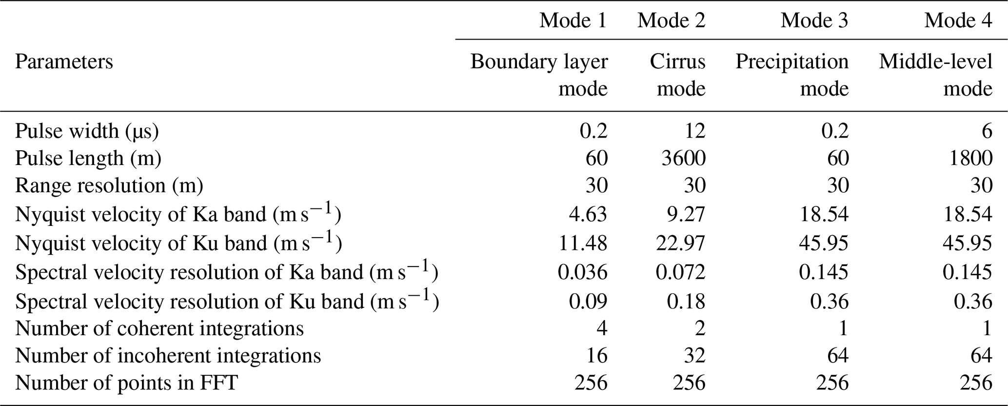
The vertically pointing Ka–Ku dual-frequency radar used in this paper has been operating at the Longmen Observation Station (114.27∘ E, 23.79∘ N; 80.3 m above mean sea level) in southeastern China since 2019. The operating parameters of four observation modes are shown in Table 1. Both radars are implemented with solid-state transmitters and pulse compression techniques. The maximum detection range is 15 km with a range resolution of 30 m. The antenna beamwidth is 0.9∘ for the Ku-band radar and 0.35∘ for the Ka band. Both radars operate with four modes: boundary layer mode (mode 1), cirrus mode (mode 2), precipitation mode (mode 3), and middle-level mode (mode 4). These four modes are characterized by different pulse compression ratios and numbers of coherent integration as well as incoherent integration. The boundary layer mode aims to detect low-level clouds and a narrower pulse waveform as well as a larger number of coherent integrations is used to improve the detection ability. The cirrus mode uses the pulse compression technique to improve the sensitivity to detect clouds with weaker radar echoes at higher altitudes. The middle-level mode also uses pulse compression techniques but fewer coherent integration times. The precipitation mode is characterized by a larger unambiguous range and velocity for rainfall observations. These four different modes are routinely cycled in operations, and each mode takes 7 s to finish the observation. The radar Doppler spectra are computed using a 256-point fast Fourier transform (FFT). The resolutions of spectral velocity at all modes are interpolated into 0.072 m s−1 (Ka-band radar) and 0.09 m s−1 (Ku-band radar). The spectral noise floor is determined using the Hilderbrand–Sekhon method (Hildebrand and Sekhon, 1974). It should be noted that due to the use of long pulses in mode 2 and mode 4 for both radars, the heights below 2 and 1 km are blind zones, respectively. The blind zones of modes 1 and 3 are 30 m. In addition, the Nyquist velocity of the Ka-band radar at mode 1 is 4.6 m s−1, and the observed Doppler spectrum easily gets aliased; therefore, the Ka-band radar observations at mode 1 were not used.
Table 1Operating parameters for the Ka–Ku-band cloud radar system deployed at Longmen Observation Station in southeastern China.
The cross-calibration between different modes is necessary before comparing observations at different modes. We selected the stable and weak precipitation cases, and the systematic offset in reflectivity observations was identified. For both radars, the reflectivity observations at mode 2 were used as the reference to calibrate radar data at other modes. For both radars, the reflectivity observations at mode 2 were used as the reference to calibrate radar data at other modes. The reflectivity offsets are 3.8 dB (mode 2–mode 3) and −3.6 dB (mode 2–mode 4) at Ka band. For the Ku-band radar, these values are 7.5 dB (mode 2–mode 1), −1.0 dB (mode 2–mode 3), and −2.9 dB (mode 2–mode 4). Note that we did not do the attenuation calibration, since it is out of the scope of this study.
Clutter contamination is a long-standing issue in scanning and vertically pointing radar observations. Both ground clutter and insect clutter obscure the boundary layer returns, affecting the high-order moments estimated from Doppler spectra observations (Sato and Woodman, 1982). In addition, the implementation of pulse compression techniques in modes 2 and 4 usually results in significant range sidelobes around the melting layer, which does not significantly affect Ze and V estimates but can severely degrade the estimation of spectrum width. In this section, Ku-band radar observations are used to demonstrate the spectral processing procedure for mitigating clutter contamination and range sidelobe.
3.1 Clutter mitigation
Stationary ground clutter is usually manifested as a narrow symmetric peak around 0 m s−1 (Williams et al., 2018). A commonly used approach for mitigating ground clutter signals is the interpolation of adjacent spectral powers after removing the spectral peak around 0 m s−1. Williams et al. (2018) claimed that this method is also suitable for the identification and removal of insect clutter since the insect targets also produce narrow peaks in Doppler spectra observations. We have tried to apply this approach to our radar data, but the performance is not as good as that of the Ka-band zenith-pointing radar (KAZR) deployed at Oliktok Point, Alaska. Figure 1a shows an example of the Ku-band Doppler spectrum with clutter signals present at around 0 m s−1. The clutter signals do not always present a sharp narrow peak as shown in Fig. 3 in Williams et al. (2018), and this approach does not apply to our observations. We have also found that such clutter signals appear more frequently and significantly in Ku-band radar observations than in the Ka band.
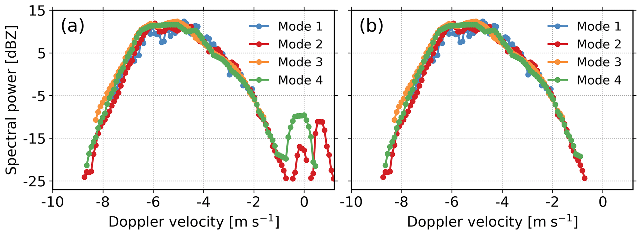
Figure 1(a) Noise-removed Ku-band Doppler power spectrum on 6 June 2020 at 22:52:08 LST at the range of 2.34 km. (b) Same as (a) but decluttered with our clutter mitigation algorithm. The unit of Doppler power spectral density data is mm6 m−3 (m s; we simply use the unit “dBZ” here and after to denote spectral power in the dB scale.
Figure 2 shows the time series of Doppler velocity spectra on 6 June 2020 from 22:40 to 23:01 LST at 2.34 km range (the same range bin as Fig. 1). The clutter signals are in the vicinity of 0 m s−1 and are not continuous with time. Compared with meteorological signals, it appears that clutter echoes randomly occur with some dependence on the observing mode. The cause of such clutter signals is still unclear and we hesitate to attribute them to insects (Williams et al., 2018) since the spectral powers at different modes deviate from each other significantly.
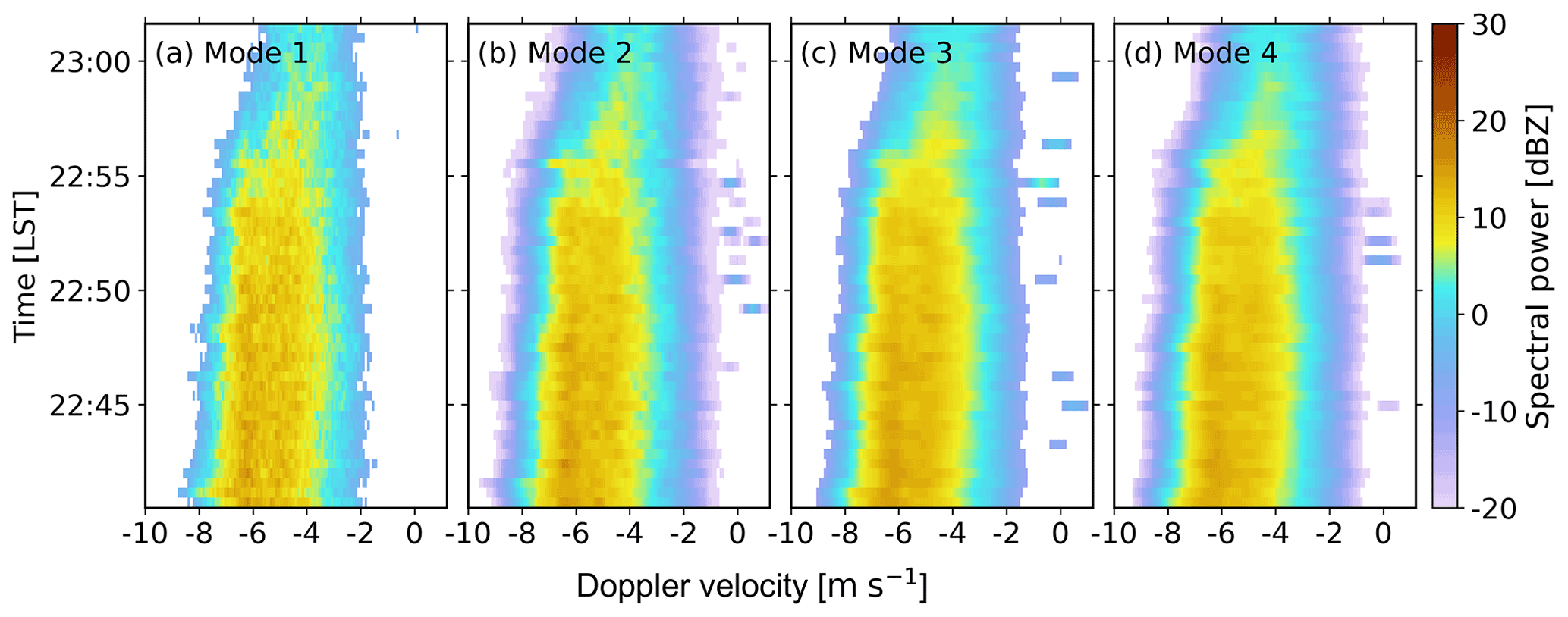
Figure 2Time series of noise-removed Ku-band Doppler velocity spectra on 6 June 2020 from 22:40 to 23:01 LST at 2.34 km range.
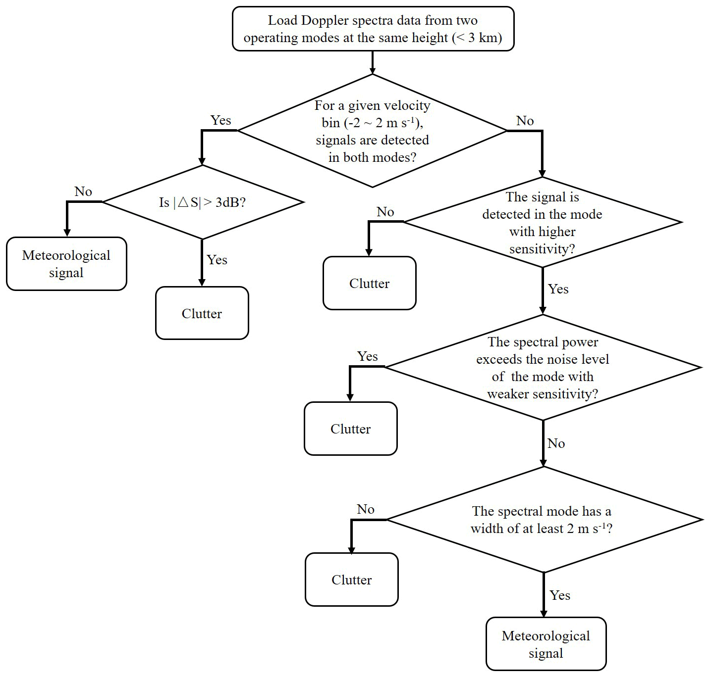
As shown in Fig. 3, we have developed an algorithm to identify and remove clutter signals. The algorithm is mainly based on the non-coherent nature of clutter, which produces a significant spectral power ratio (ΔS) between observations from different modes. The selection of the threshold is a comprise between a false alarm and miss hit. We want to preserve the meteorological signals to the best of our ability, and therefore we checked the magnitudes of for meteorological signals. Appendix A presents the statistical plot of for meteorological signals (height of 2–3 km and Doppler velocity of 2–5 m s−1). It appears that the probability of tends to be flat after 3 dB, and the use of 3 dB can ensure that 95.6 % of precipitation signals are well preserved (Fig. A1). Therefore, 3 dB is used in this study. If a larger threshold is employed, we expect more clutter signals will be mislabeled as precipitation. As shown in Fig. 1b, clutter signals have been successfully removed, while the meteorological signals are marginally affected.
It should be noted that this method relies on observations recorded at different observing modes. However, the sensitivities of different modes are not identical. Therefore, if the clutter is presented in the most sensitive mode (e.g., mode 2) only, it cannot be filtered out with the method. In this case, the width of a valid meteorological spectral mode is assumed to be longer than 2 m s−1; otherwise, it is attributed to clutter. We are aware that Shupe et al. (2004) have used a width of 0.448 m s−1 to identify supercooled liquid water. We have tried this value, but the width of clutter present in this dual-wavelength radar system easily exceeds 1 m s−1 (Fig. 2). Actually, the selection of the spectrum width is similar with the use of a signal-to-noise ratio (SNR) value in noise removal. A higher SNR means stricter noise removal but higher chance of losing valid signals. We have tested the width of 1, 1.5, 2, and 3 m s−1 (visual inspection, not shown) and found that 2 m s−1 can effectively remove clutter signals for both radars, though very light precipitation (detected by the most sensitive mode only) can be removed as well. Admitting this potential issue, it suffices for the application in rainfall. In addition, for clouds with highly variable reflectivity, the presented algorithm may mislabel them as clutter according to our assumption that meteorological signals are coherent in a round of observation (28 s).
Figure 4 compares the Doppler spectrum observations before and after applying the declutter algorithm. As shown in Fig. 4a1 and c1, the clutter signals appear below 2 km at modes 1 and 3. For modes 2 and 4, the impact of clutter can be up to 3 km (Fig. 4b1 and d1). After imposing the declutter algorithm, no significant clutter signals can be detected (Fig. 4a2, b2, c2, and d2).
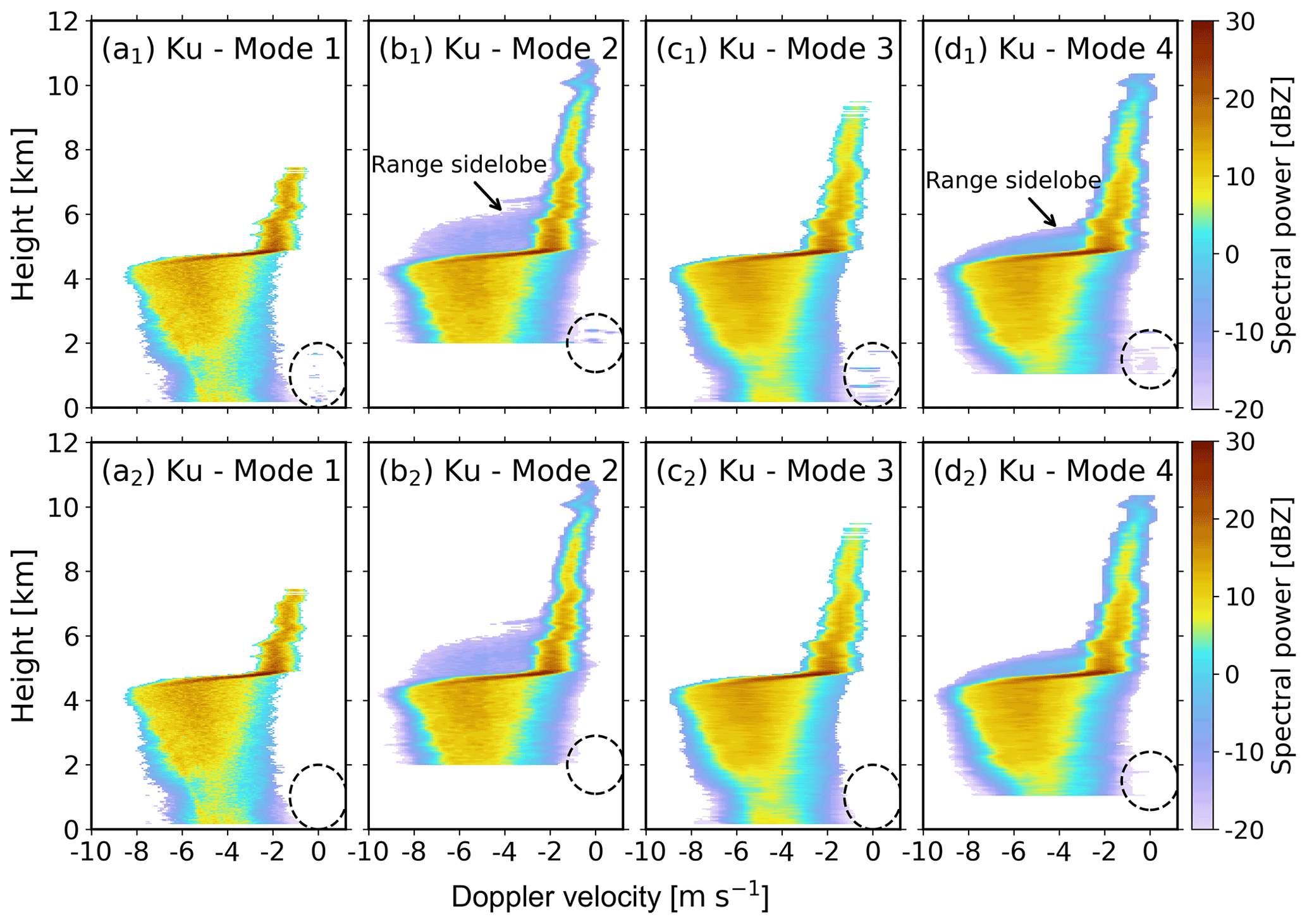
Figure 4(a1–d1) Noise-removed Ku-band Doppler power spectra on 6 June 2020 at 22:52:08 LST recorded at (a1) mode 1, (b1) mode 2, (c1) mode 3, and (d1) mode 4. (a2–d2) Decluttered observations. The dashed circles mark the clutter signals. Note that the heights below 2 and 1 km are blind zones for modes 2 and 4, respectively.
3.2 Range sidelobe artifacts
The utilization of pulse compression usually leads to significant range sidelobe artifacts (Fig. 4b1 and d1) around the melting layer, which can severely affect the estimates of high-order radar moments. Moran has proposed an approach that distinguishes the range sidelobe artifacts from reflectivity data using non-range-corrected return power through the power transfer function (Moran et al., 1998; Clothiaux et al., 1999). By reducing the number of code bits used in pulse compression modes, the ARM MMCRs' upgraded processor is capable of suppressing the range sidelobe effects (Moran et al., 2002). However, mitigating range sidelobe artifacts is still challenging for multi-mode pulsed compression cloud radars in China. To improve both the radar detection performance and range resolution, linear frequency modulation was used to widen the signal bandwidth when transmitting pulses in modes 2 and 4 at both Ka and Ku band. But, the matched pulse compression filter output exhibits sidelobe behavior, making the power of range sidelobe appear in the wrong range gates. Liu and Zheng (2019) have applied the method proposed by Moran et al. (1998) to radar Doppler spectrum data to remove the range sidelobe artifacts. However, the performance of this approach depends on a given threshold, which needs to be adjusted for different scenarios.
As shown in Fig. 4b1 and d1, the range sidelobe associated with the strong radar echoes of melting particles is located above the melting layer. Compared with radar Doppler spectrum observations without the sidelobe contamination (see, for example, Li and Moisseev, 2020), Doppler spectra above the melting layer at large velocity bins were contaminated by the range sidelobe of the echo below. The artifacts in mode 2 accumulate to higher altitudes but are weaker in spectral power (Fig. 4b1), while mode 4 accumulates to lower altitudes and with a larger magnitude of power (Fig. 4d1), which is caused by the different pulse compression ratio and peak sidelobe ratio (the ratio of the main lobe peak power to the highest sidelobe peak power) of the two modes.
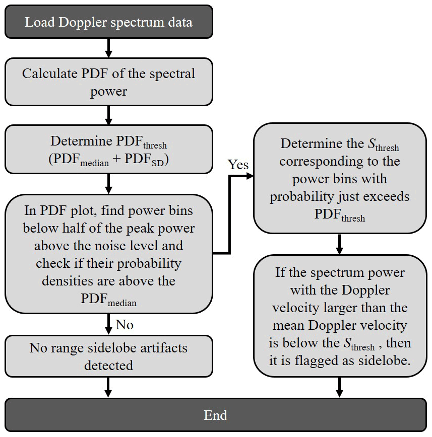
An interesting feature of the range sidelobe caused by pulse compression is that its spectral power is much flatter than cloud and precipitation signals. Figure 5a shows the probability density functions (PDFs) of received spectral power at 2.4, 5.01, and 6.6 km, which respectively represent the liquid precipitation, Doppler spectrum contaminated by range sidelobe, and solid precipitation. For the sidelobe-contaminated Doppler spectrum, it can be seen that the range bins contaminated by range sidelobe have different spectral power distributions; the peak of the PDFs appears close to the noise level and is mostly below 15 dB above the noise level. A closer look into the radar Doppler spectra at 5.01 km (Fig. 6a) shows that the strong PDF peak in Fig. 5b is explained by the relatively flat range sidelobe signals. Here, we introduce a parameter called the spectral power threshold (Sthresh) to distinguish the range sidelobe from meteorological signals. Figure 7 shows the flowchart for the identification and removal of the range sidelobe artifacts. The procedures are briefly summarized as follows.
-
Sort the spectral power values above noise level in ascending order to get a PDF curve of each Doppler spectrum.
-
Calculate the median and standard deviation (SD) of the PDFs, and set PDFthresh= PDFmedian+ PDFSD; note that the determination of this relation is given in Appendix B.
-
Below half of the peak power above the noise level of the Doppler spectrum, find the power bins' probability density that just exceeds the PDFthresh, and the corresponding spectral power is set as Sthresh. (The range of PDFthresh is limited to half of the peak power above the noise level to avoid finding the PDFpeak corresponding to large spectral power, which makes the determined Sthresh correspond well to the power of sidelobe in this way.)
-
If the spectrum power with the Doppler velocity larger than the mean Doppler velocity is below the Sthresh, then it is flagged as sidelobe.
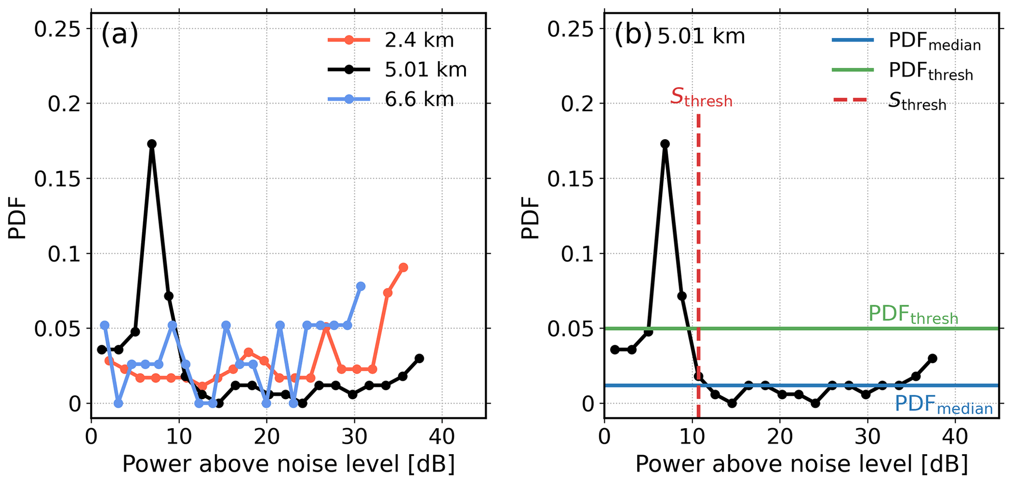
Figure 5(a) PDFs of Doppler spectra from 2 to 7 km at mode 2; (b) PDF of Doppler spectrum recorded at 5.01 km.
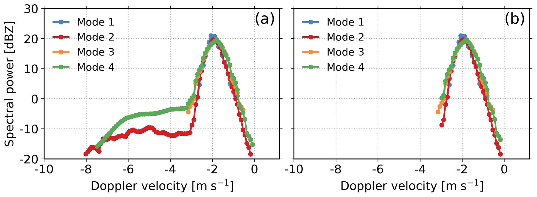
Figure 6Ku-band Doppler power spectra recorded at different modes at 5.01 km on 6 June 2020 at 22:52:08 LST. (a) Noise-removed Doppler spectrum; (b) the same as (a) but after the removal of range sidelobe.
As shown in Fig. 6b, the range sidelobe artifacts in modes 2 and 4 have been removed well. We have applied this algorithm to the vertical profiles of Doppler spectra observations at modes 2 and 4 (Fig. 4b1 and d1). As shown in Fig. 8, the sidelobe artifacts have been removed well at modes 2 and 4. Furthermore, we have compared this algorithm with the threshold method (Liu and Zheng, 2019), and all the results and analysis are included in Appendix C.
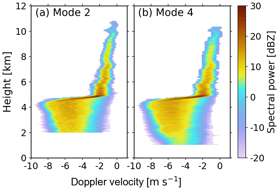
Figure 8Doppler power spectra after removing range sidelobe at modes 2 and 4 on 6 June 2020 at 22:52:08 LST. The Doppler spectra observations before the sidelobe removal are shown in Fig. 4b1 and d1.
For multi-mode cloud radars, it is cumbersome to interpret the radar observations recorded at four modes in operational applications. Moreover, the air motion variability and the velocity bin-to-bin spectrum power fluctuations can lead to noisy estimates of high-order spectral moments. Therefore, we have merged radar observations from different observing modes. Data from the Ku band were still taken as an example to illustrate the data merging process.
4.1 Merging of Doppler spectra recorded at different modes
Before the merging procedure, it is necessary to check the consistency of radar data at four modes. Particularly, coherent integrations were made to modes 1 and 2 (Table 1) to improve the signal-to-noise ratio. But this step may result in a decrease in spectral power with large Doppler velocities (Liu et al., 2017; Liu and Zheng, 2019). This effect leads to the underestimation of V, which is critical in the merging process, and Ze. Here, we evaluate this impact by comparing Ze and V estimates at different modes. We define the differences of Ze and V between different modes as ΔZ and ΔV, respectively, and radar observations at mode 3 (no pulse compression and only one round of coherent integration were performed) were used as a reference. To compare the impact of coherent integration under various precipitation intensities, radar observations were grouped into Ze>20 dBZ and Ze<10 dBZ. Note that the Ku-band wet radome attenuation has been corrected with a collocated C-band radar (Cui et al., 2020).
In light precipitation (Ze<10 dBZ, Fig. 9a1, b1, and c1), radar observations at these four modes agree with each other rather well. For precipitation cases with Ze>20 dBZ, good agreement between modes 3 and 4 can also be found (Fig. 9c2), which is expected since the coherent integration number is 1 at both modes. The agreement between modes 2 and 3 also seems good (Fig. 9b2), despite two rounds of coherent integration being made to mode 2. In Fig. 9a2, significant biases of ΔZ and ΔV can be identified, and ΔV increases with ΔZ. This is attributed to the underestimation of spectrum powers at high Doppler velocities during the long-time coherent integration (four rounds). Given the results above, Ku-band Doppler spectra observations at mode 1 were discarded.
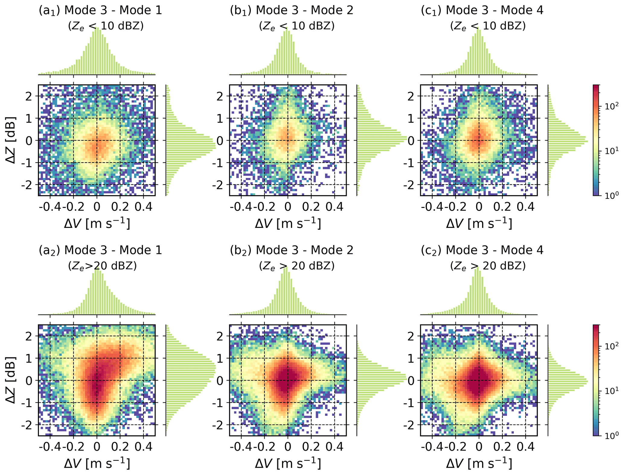
Figure 9Statistics of ΔZ and ΔV for the Ku-band radar. (a1–c1) Precipitation cases with Ze<10 dBZ; (a2–c2) precipitation cases with Ze>20 dBZ.
The same method was applied to the Ka-band radar (Fig. 10). Note that the data from mode 1 were not used due to the small Nyquist velocity (4.63 m s−1 as shown in Table 1). Interestingly, 2 times the coherent integration marginally affects ΔZ and ΔV for the Ku-band radar data (Fig. 9b2), but this impact is rather significant at Ka band (Fig. 10a2). Therefore, Ka-band radar observations from both modes 1 and 2 were not used.
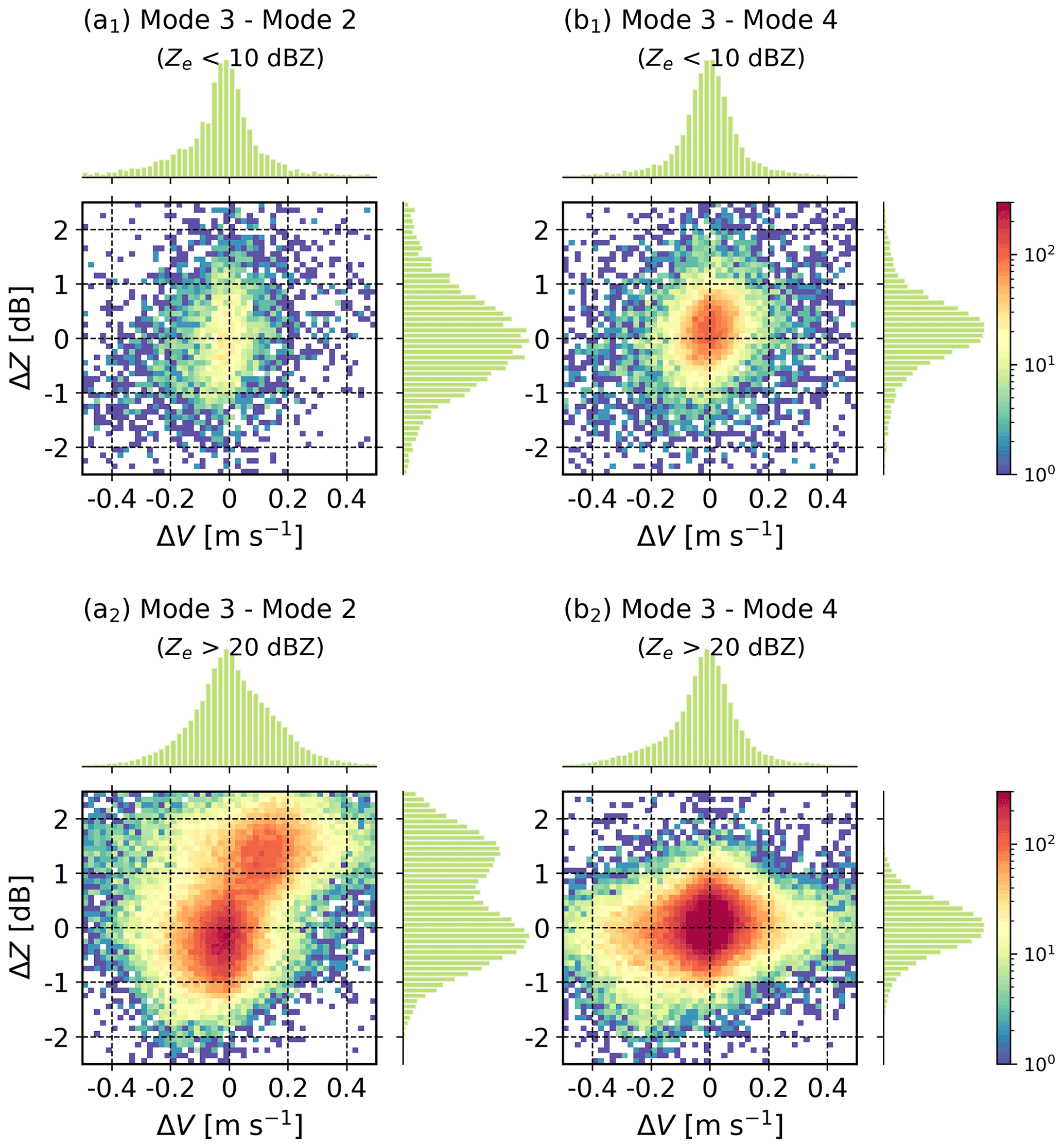
Figure 10Same as Fig. 9 but for the Ka-band radar. Note that the data at mode 1 were excluded due to the limited Nyquist velocity.
4.2 Shift-then-average spectra
To maximize the detection advantages of each mode and to obtain high-quality and easy-to-use radar datasets, Doppler spectra observations from various modes were merged as follows (Giangrande et al., 2001; Luke and Kollias, 2013; Williams et al., 2018).
-
Velocity shift: set the mean of the mean Doppler velocity at each mode as the reference velocity, and then shift the Doppler spectrum at each mode to match the mean Doppler velocities at all modes.
-
Spectral power average: average the spectral powers observed at all modes in each observation round.
For the Ku-band radar, observations at modes 2, 3, and 4 were merged (Fig. 11a), while modes 3 and 4 were used for the Ka-band radar (Fig. 11b). The merged Doppler spectrum is significantly less uncertain thanks to the averaging process. It should be noted that the drawback of the mode merging is that the time resolution changes from 7 to 28 s.
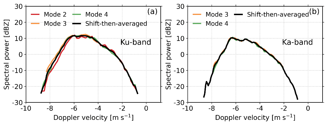
Figure 11(a) Ku-band Doppler velocity spectra from modes 2, 3, and 4 recorded on 6 June 2020 at 22:52:08 LST at 2.34 km. The merged Doppler spectrum was derived from the Doppler spectra recorded at modes 2, 3, and 4 after shifting and averaging. Note that Ku-band radar observations at mode 1 were not used due to the power loss during coherent integration. (b) The same as in (a) but for Ka-band, and observations at modes 3 and 4 were used.
High-order moments of the Doppler spectrum are representative of the key microphysical processes in clouds and precipitation (Luke and Kollias, 2013; Maahn and Löhnert, 2017; Li et al., 2021). The second, third, and fourth moments of the radar Doppler spectrum are spectrum width, skewness, and kurtosis, respectively. Figure 12 compares these high-order moments estimated from the Ku-band radar Doppler spectra at modes 2, 3, and 4, as well as the merged data. The sidelobe impacts on spectrum width, skewness, and kurtosis are significant between 5 and 7 km at modes 2 and 4 (Fig. 12a–c). In rain, the estimates of high-order moments at modes 2, 3, and 4 agree rather well with each other. In snow, the spectrum width at mode 2 is systematically smaller than those at other modes (Fig. 12a). This may be explained by the finer spectral velocity resolution at mode 2 (Table 1). In addition, as the radar echo approaches the noise level, underestimation of kurtosis becomes more significant (mode 3 in Fig. 12c).

Figure 12(a) Spectrum width, (b) skewness, and (c) kurtosis estimated from Ku-band radar Doppler spectra recorded at modes 2, 3, and 4, as well as the merged data; (d) the profile of merged Doppler velocity spectra. Note that Ku-band radar observations at mode 1 were not used due to the power loss during coherent integration.
The results for the Ka-band radar are shown in Fig. 13. The agreement among different modes is better than that at Ku band thanks to higher spectral velocity resolution and fewer uncertainties for the Ka-band radar, while the bias of kurtosis in the snow at mode 3 (Fig. 13c) is more contrasting. These findings indicate that the uncertainties of estimated radar moments as introduced by different observing modes should be taken into account in snow retrievals (Maahn and Löhnert, 2017).
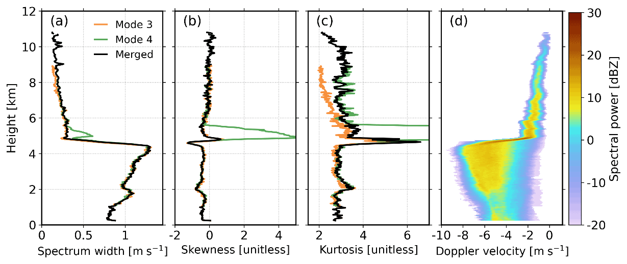
Figure 13Same as Fig. 12 but for the Ka-band radar. Note that Ka-band radar observations at mode 1 were not used due to the limited Nyquist velocity, while mode 2 data were discarded due to the power loss during coherent integration.
The presented methods were used to construct a new spectra-based radar data processing framework as shown in Fig. 14. In this section, we take a rainfall event to illustrate the algorithms presented in this study. On 6 June 2020, a stratiform rainfall system moved over the Longmen station. The melting layer is about 5 km, and the bright band signatures can be identified well from Ku- and Ka-band radar reflectivity observations as shown in Figs. 15 and 16.
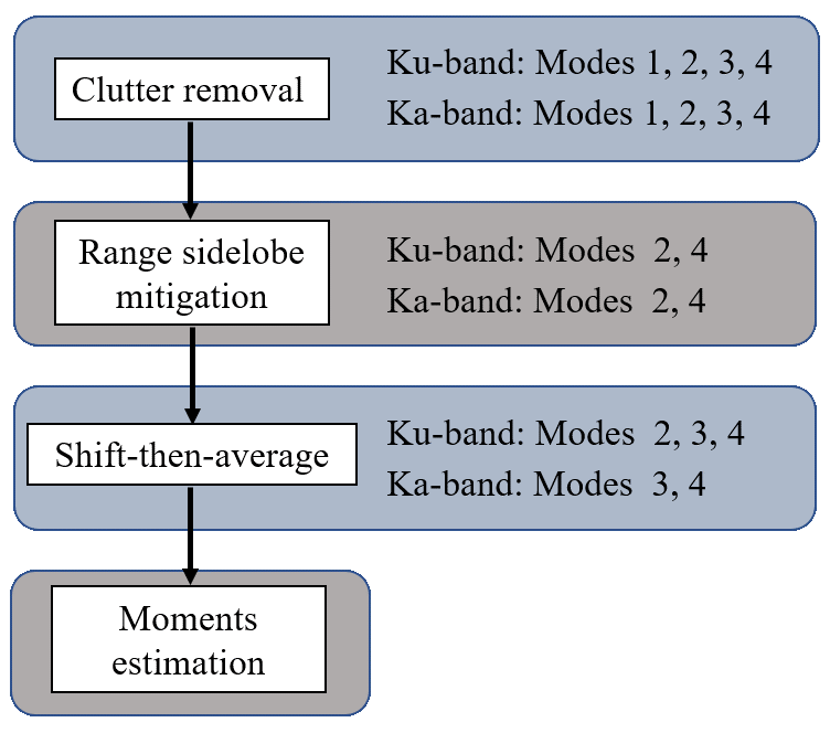
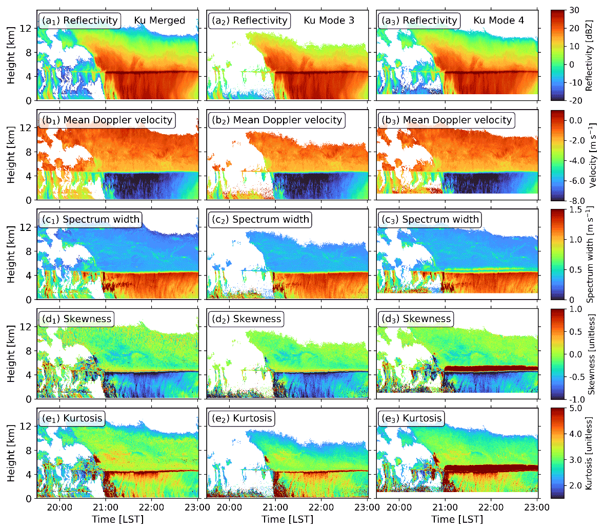
Figure 15Time–height cross-section plots of Ku-band Doppler spectra moments from 19:30:19 to 23:01:26 LST. The left column (a1–e1) is estimated from the merged Doppler spectra, and the middle (a2–e2) and right (a3–e3) columns are from the data recorded at modes 3 and 4, respectively. From top to bottom: (a1–a3) reflectivity; (b1–b3) mean Doppler velocity; (c1–c3) spectrum width; (d1–d3) skewness; (e1–e3) kurtosis.


Figure 17Spectrum width comparison between C band, (a1, a2) Ku band, and (b1, b2) Ka band. The spectrum width observations at mode 4 (a1, b1) and for merged data (a2, b2) were used for comparison. Radar observations from 1 to 9 km during this event were employed.
5.1 Case study
To evaluate the performance of the presented framework, the merged radar products were compared with raw data products at modes 3 and 4 after processing the Ku- and Ka-band data with the proposed algorithm. The time–height cross-section plots of Ku- and Ka-band radar observations are shown in Figs. 15 and 16, respectively. The cloud-top height is about 14 km (Fig. 15a1), while it is much lower at mode 3 (9–10 km), which is attributed to the lower sensitivity at this mode. At Ka band, due to the increased attenuation from rain, the melting layer, and the wet radome (Li and Moisseev, 2019), the observed cloud top descends to around 7 km during the most intensive precipitation period (around 22:00 LST, Fig. 16a2). The bias in spectrum width, skewness, and kurtosis introduced by sidelobe effect is rather significant at mode 4 for both radars (Figs. 15c3–e3 and 16c3–e3), while it was well mitigated in the merged products (Figs. 15c1–e1 and 16c1–e1).
In addition, we have calculated statistics of the power leakage to range sidelobe, and the results for Ku–Ka-band radars are given in Appendix D (Fig. D1). The results show that the sidelobe signals are usually below −20 dB. Since the reflectivity enhancement in the melting layer usually does not exceed 10 dB (Li et al., 2020), the sidelobe contamination in rain is not significant. However, the fall velocity of snow is much slower than raindrops. Namely, no meteorological signals are present in the range of 3–10 m s−1, and the sidelobe signal becomes evident.
Skewness and kurtosis are indicative of the degree of asymmetry and peakness of the spectrum, respectively. Skewness has been used as an early qualitative predictor of drizzle onset in clouds and locating supercooled liquid water since it is very sensitive to drizzle generation (Luke et al., 2010; Kollias et al., 2011a, b). Higher-order radar moments have been less frequently used for studying the melting layer. It appears that skewness presents a “decrease–increase–decrease” feature, while kurtosis is characterized by a distinct enhancement. These observations of skewness and kurtosis in the melting layer are interesting, and how these changes are linked to the change in cloud and precipitation microphysics warrants future studies.
5.2 Comparison with a C-band radar
Observations from a collocated C-band frequency-modulated continuous wave radar (FMCW) radar (Cui et al., 2020) were used for a sanity check for the processed Ka–Ku-band radar data products. The C-band radar's data products include reflectivity, Doppler velocity, and spectrum width. The spectrum width observed by the C-band radar was compared with those from mode 4 of Ku- and Ka-band radars. As shown in Fig. 17a1 and b1, the surge of Ku- and Ka-band spectrum width at around 0.4 m s−1 is attributed to the sidelobe effect, while the artifacts were well mitigated after applying the presented algorithm (Fig. 17a2 and b2). It is interesting to note that the observed spectrum width at Ku–Ka band does not necessarily follow the 1:1 line, since the Rayleigh scattering may not be satisfied at Ku–Ka band for heavy precipitating cases.
5.3 Quantitative evaluation
This precipitation event is also used for quantitative evaluations of the presented methods. Spectral moments (reflectivity, Doppler velocity, spectrum width, skewness, and kurtosis) before and after the spectral processing are quantitatively compared to show the effectiveness and necessity of the presented methods. The results of clutter and sidelobe mitigation are presented in separate subsections.
5.3.1 Clutter removal
To show how the clutter mitigation procedure improves the radar data quality, we have compared the standard deviation between the data products before and after the clutter removal and the “reference data”. At Ku band, the reference data are defined as
where denotes the spectral moment derived from decluttered Doppler spectra at mode i. Similarly, the reference data at Ka band are
We introduce the standard deviation to assess the difference between radar products at a given mode and the reference data:
where m denotes the number of rainfall cases between 0 and 3 km. The results for the Ku- and Ka-band radar during this event are given in Tables 2 and 3, respectively.
Table 2Standard deviation (SD) for Ku-band spectral moments before and after the declutter approach compared with the reference data. Radar observations from 0 to 3 km are used for comparison.
As we can see from Table 2, clutter signals affect the estimation of spectral moments, and the SD for the reflectivity at Ku band is reduced by a value between 0.36 and 0.8 dB after imposing the clutter removal algorithm. Significant improvement can also be identified for mean Doppler velocity and spectrum width observations. Compared with the Ku-band radar, clutter signals are weaker at Ka band (Table 3). The data quality improvement of spectral moments at the Ka band is not as pronounced as that at Ku band, which is expected since the Ka-band radar's beamwidth (0.35∘) is smaller than that of the Ku band (0.9∘). The presented results indicate that clutter removal is essential for producing high-quality Ku data products.
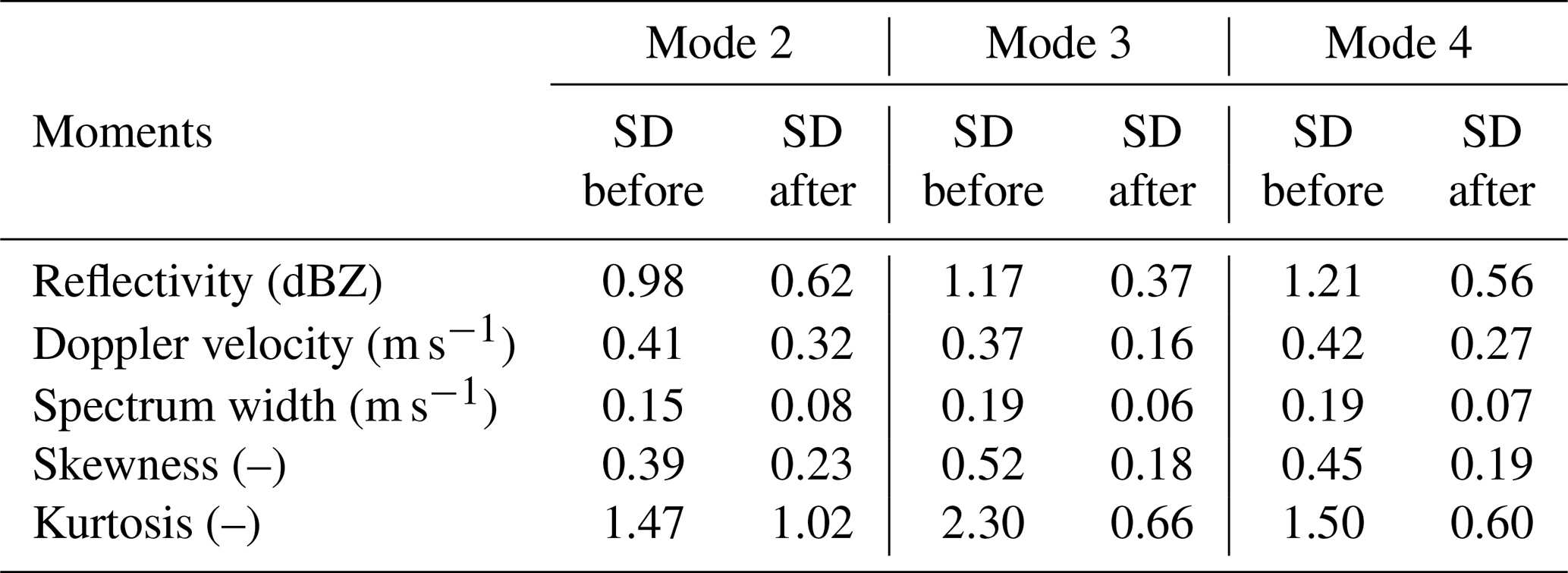
5.3.2 Sidelobe mitigation
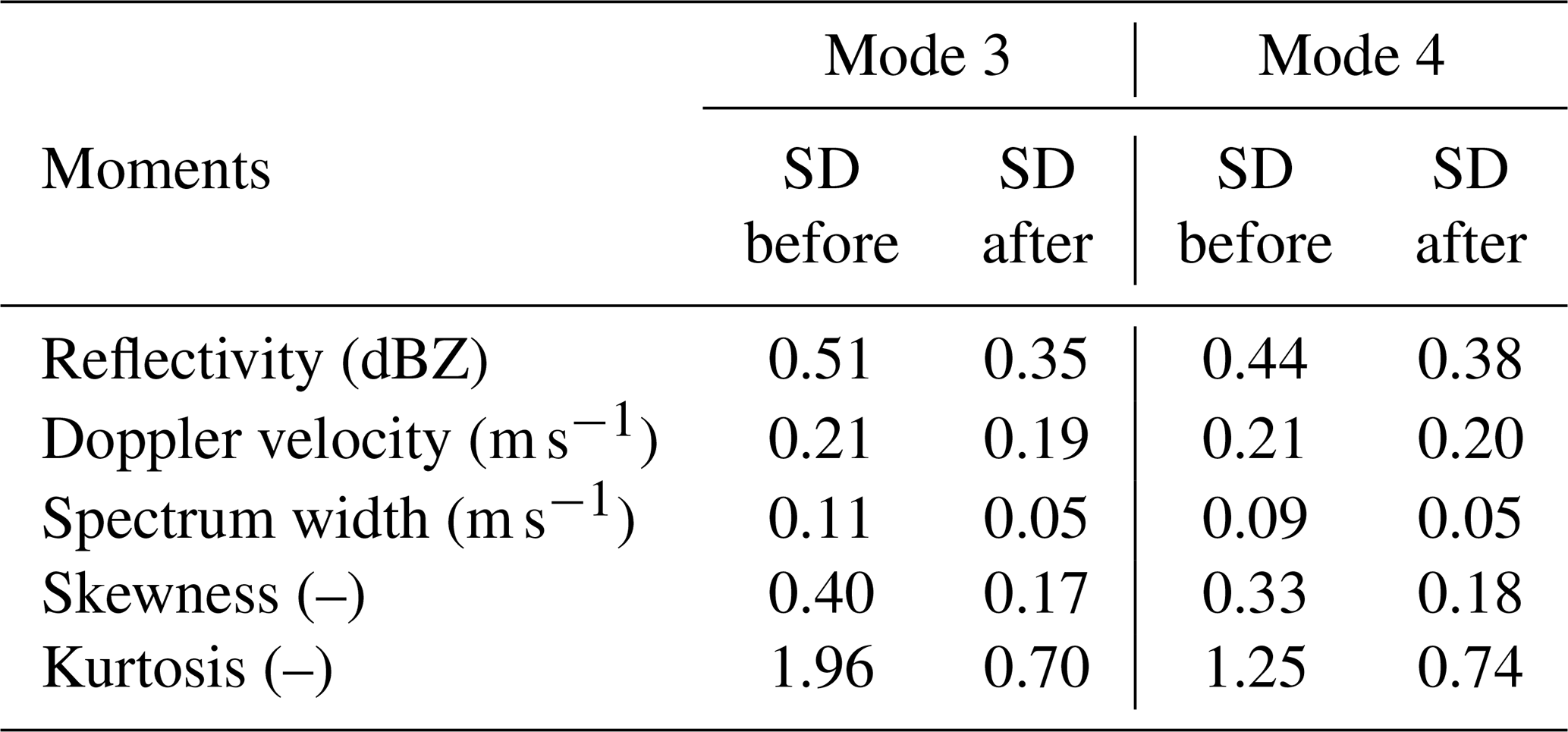
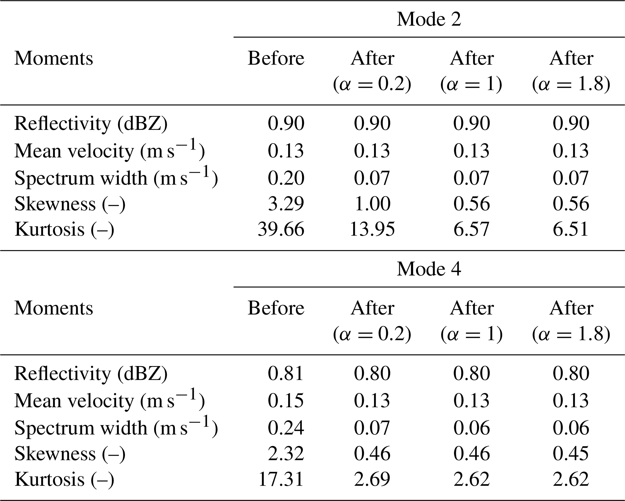
The effect of sidelobe mitigation was also quantitatively evaluated. Since no pulse compression was employed at mode 3 for the Ka–Ku-band radars, we use radar data products at mode 3 as reference data. Radar observations from 4.5 to 6 km are used for the assessment, and the results for the Ku-band radar are given in Appendix B (see Table B1 for details). Since the signals associated with sidelobe are relatively weak (Fig. D1 in Appendix D), no significant changes in reflectivity and mean Doppler velocity before and after sidelobe suppression can be identified in both modes 2 and 4. As the order of spectral moments increases, the effect of range sidelobe becomes significant. The SD values of spectrum width are reduced by an order of magnitude after the sidelobe mitigation at both modes 2 and 4. Moreover, the improvement of skewness and kurtosis after the sidelobe mitigation is more obvious. The Ku-band SD of skewness at mode 2 (mode 4) decreased from 2.88 (0.4) to 1.61 (0.26), and that of kurtosis decreased from 31.38 (5.4) to 11.64 (1.32). Similar improvement in skewness and kurtosis can also be found at Ka band (Table B2 in Appendix B).
In this study, a framework for processing the Doppler spectra observations of a multi-mode pulse compression Ka–Ku cloud radar system is presented. We first proposed an approach to identify and remove the clutter signals in the Doppler spectrum based on spectral power ratios between different operating modes. Then, we developed a new algorithm to remove the range sidelobe around the melting layer at the modes implementing the pulse compression technique. We further show that coherent integration has a decent impact on reflectivity and Doppler velocity observations and should be used with caution when the spectral merging is made. The radar observations from different modes were then merged using the shift-then-average method. The presented spectral processing framework was applied to radar observations of a stratiform precipitation event, and the quantitative evaluations of the processed data suggest that clutter or sidelobe suppression and spectral merging results demonstrated good performance.
The presented methods mainly deal with the challenges in observing stratiform rainfall events in southern China, given the weaker signal attenuation at both bands compared with that in convective precipitation. We are aware that cloud radars have proven to be an effective tool for snowfall observations (e.g., Kollias et al., 2007; Li et al., 2021), and the applicability of the presented framework in snowfall is expected but has not been proven yet. The multiyear radar observations recorded at the Longmen station will be processed with the present framework for elucidating the dynamics and microphysics of clouds and precipitation in southern China.
The meteorological signals with a height of 2–3 km and Doppler velocity of 2–5 m s−1 were statistically analyzed to determine the appropriate .

Figure A1(a) Probability density and (b) cumulative distribution of the spectral power ratio of meteorological signals between different modes at Ku band.
Here, we define PDFthresh= PDFmedian+α PDFSD. By varying α, different values of PDFthresh can be obtained. A similar quantitative evaluation can be made to find the appropriate value of α to maximize the sidelobe mitigation. Since the Doppler spectra observations at mode 3 for both radars are not affected by the sidelobe effect, they are used as the reference data at both Ku and Ka band. That is,
Then, the standard deviation between spectral moments with different α and observations at mode 3 was calculated through Eq. (B1) and compared. Radar observations between 4.5 and 6 km were evaluated, and the results for Ku- and Ka-band radars are given in Tables B1 and B2, respectively. As we can see, the sidelobe artifacts have a minimized impact on reflectivity and mean Doppler velocity observations. After applying the PDF method, smaller standard deviation values can be found for spectrum width, skewness, and kurtosis. In addition, the performance of the PDF method depends on the selection of α. The value of 1 seems to yield the best results. Smaller α (e.g., 0.2) may mislabel sidelobe signals as meteorological echoes, while larger α (e.g., 1.8) may not able to fully remove sidelobe signals. We have also tried other values such as 0.8 and 1.2 for α and found rather similar results with the use of 1. This demonstrates that α=1 seems to be robust.
Table B1Standard deviation (SD) for Ku-band spectral moments before and after the sidelobe removal compared with observations at mode 3. Radar observations from 4.5 to 6 km are used for comparison.
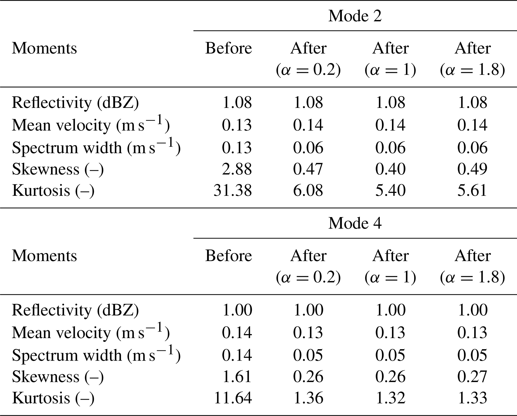
Table B2Standard deviation (SD) for Ka-band spectral moments before and after the sidelobe removal compared with observations at mode 3. Radar observations from 4.5 to 6 km are used for comparison.
This Appendix shows the comparison of the presented sidelobe mitigation algorithm (PDF method) with the threshold method (Liu and Zheng, 2019). The range sidelobe caused by pulse compression technology appears in both the upper and lower range gates of the target bin, which is weaker compared with the echo of the target. At Ku band, the theoretical peak sidelobe ratio (the ratio of the main lobe peak power to the highest sidelobe peak power) is 36 and 30 dB for mode 2 and mode 4, respectively. Figure C1 shows the comparison of sidelobe mitigation effects of the threshold method and the PDF method. The implementation of theoretical thresholds (Fig. C1a1 and b1) is insufficient to remove sidelobe signals. However, a smaller threshold may remove valid signals (Fig. C1a3 and b3). This effect is more evident in the zoomed-in plot (Fig. C2). In contrast, our algorithm is an adaptive method that efficiently removes sidelobe signals with the valid signal well preserved (Figs. C1a4 and b4 and C2a4 and b4).
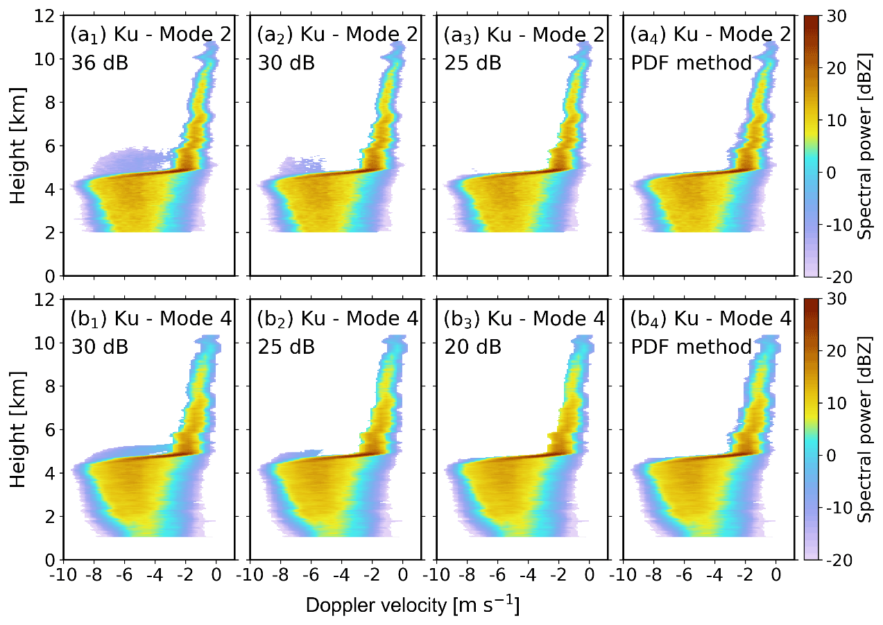
Figure C1Ku-band Doppler power spectra after mitigating range sidelobe at modes 2 and 4 after the sidelobe mitigation using the threshold method (a1–a3, b1–b3) and PDF method (a4, b4) on 6 June 2020 at 22:52:08 LST. The Doppler spectra observations before the sidelobe mitigation can be found in Fig. 4b1 and d1.
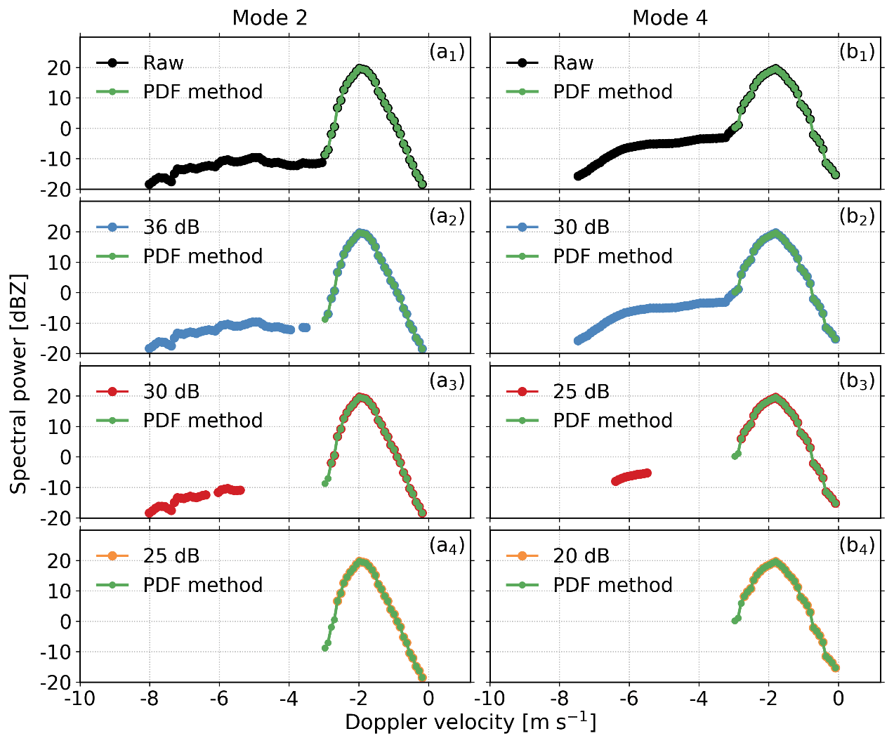
Figure C2Ku-band Doppler power spectra recorded at (a1–a4) modes 2 and (b1–b4) 4 at 5.01 km after the sidelobe mitigation using the threshold method and PDF method on 6 June 2020 at 22:52:08 LST.
This Appendix shows how much power is leaking into the range sidelobes. For a given velocity bin in a spectra profile, the maximum spectral power is denoted as Speak, and the corresponding height is Hpeak. Then, the sidelobe spectral power is denoted as Ssidelobe and the height as Hsidelobe. The difference between Speak and Ssidelobe and the corresponding Hpeak and Hsidelobe were analyzed. As can be seen in Fig. C1, the patterns of range sidelobes at modes 2 and 4 are different due to their different pulse compression ratios.
The theoretical peak sidelobe ratio (the ratio of the main lobe peak power to the highest sidelobe peak power) depends on the transmitted waveform after pulse compression and is 36 and 30 dB for modes 2 and 4, respectively. Therefore, the sidelobe of mode 2 is weaker than that of mode 4. At the height close to Hpeak, the power difference between Ssidelobe and Speak can be much higher than the theoretical value due to the overlap of multiple sidelobes.

Figure D1Statistical distribution of range sidelobe power as a function of heights at Ku band (a1, b1) and Ka band (a2, b2).
The data used in this study can be made available upon request to the corresponding author.
HL and LL conceptualized this study; HD performed the investigation and co-wrote the draft with HL. All authors contributed to reviewing and editing the paper.
The contact author has declared that none of the authors has any competing interests.
Publisher's note: Copernicus Publications remains neutral with regard to jurisdictional claims in published maps and institutional affiliations.
This research has been supported by the National Natural Science Foundation of China (grant no. 41875036), National Key Research and Development Program of China (grant no. 2017YFC1501703), National Natural Science Foundation of China (grant nos. 42105141 and U2142210), the Basic Research Fund of CAMS (grant no. 451490), and the Postgraduate Research & Practice Innovation Program of Jiangsu Province (grant no. KYCX22_1153).
This paper was edited by Stefan Kneifel and reviewed by three anonymous referees.
Clothiaux, E. E., Moran, K. P., Martner, B. E., Ackerman, T. P., Mace, G. G., Uttal, T., Mather, J. H., Widener, K. B., Miller, M. A., and Rodriguez, D. J.: The Atmospheric Radiation Measurement Program Cloud Radars: Operational Modes, J. Atmos. Ocean. Tech., 16, 819–827, https://doi.org/10.1175/1520-0426(1999)016<0819:Tarmpc>2.0.Co;2, 1999.
Cui, Y., Ruan, Z., Wei, M., Li, F., and Ge, R.: Vertical structure and dynamical properties during snow events in middle latitudes of China from observations by the C-band vertically pointing radar, J. Meteorol. Soc. Jpn. Ser. II, 98, 527–550, https://doi.org/10.2151/jmsj.2020-028, 2020.
Giangrande, S. E., Babb, D. M., and Verlinde, J.: Processing Millimeter Wave Profiler Radar Spectra, J. Atmos. Ocean. Tech., 18, 1577–1583, https://doi.org/10.1175/1520-0426(2001)018<1577:Pmwprs>2.0.Co;2, 2001.
Hildebrand, P. H. and Sekhon, R.: Objective determination of the noise level in Doppler spectra, J. Appl. Meteorol., 13, 808–811, 1974.
Hu, X., Ge, J., Du, J., Li, Q., Huang, J., and Fu, Q.: A robust low-level cloud and clutter discrimination method for ground-based millimeter-wavelength cloud radar, Atmos. Meas. Tech., 14, 1743–1759, https://doi.org/10.5194/amt-14-1743-2021, 2021.
Illingworth, A. J., Hogan, R. J., O'Connor, E. J., Bouniol, D., Brooks, M. E., Delanoé, J., Donovan, D. P., Eastment, J. D., Gaussiat, N., Goddard, J. W. F., Haeffelin, M., Baltink, H. K., Krasnov, O. A., Pelon, J., Piriou, J.-M., Protat, A., Russchenberg, H. W. J., Seifert, A., Tompkins, A. M., van Zadelhoff, G.-J., Vinit, F., Willén, U., Wilson, D. R., and Wrench, C. L.: Cloudnet: Continuous Evaluation of Cloud Profiles in Seven Operational Models Using Ground-Based Observations, B. Am. Meteorol. Soc., 88, 883–898, https://doi.org/10.1175/bams-88-6-883, 2007.
Kalapureddy, M. C. R., Sukanya, P., Das, S. K., Deshpande, S. M., Pandithurai, G., Pazamany, A. L., Ambuj K., J., Chakravarty, K., Kalekar, P., Devisetty, H. K., and Annam, S.: A simple biota removal algorithm for 35 GHz cloud radar measurements, Atmos. Meas. Tech., 11, 1417–1436, https://doi.org/10.5194/amt-11-1417-2018, 2018.
Kalesse, H., Szyrmer, W., Kneifel, S., Kollias, P., and Luke, E.: Fingerprints of a riming event on cloud radar Doppler spectra: observations and modeling, Atmos. Chem. Phys., 16, 2997–3012, https://doi.org/10.5194/acp-16-2997-2016, 2016.
Kneifel, S., Kollias, P., Battaglia, A., Leinonen, J., Maahn, M., Kalesse, H., and Tridon, F.: First observations of triple-frequency radar Doppler spectra in snowfall: Interpretation and applications, Geophys. Res. Lett., 43, 2225–2233, 2016.
Kollias, P., Albrecht, B. A., and Marks, F., Jr.: Why Mie?, B. Am. Meteorol. Soc., 83, 1471–1484, https://doi.org/10.1175/bams-83-10-1471, 2002.
Kollias, P., Clothiaux, E. E., Miller, M. A., Albrecht, B. A., Stephens, G. L., and Ackerman, T. P.: Millimeter-Wavelength Radars: New Frontier in Atmospheric Cloud and Precipitation Research, B. Am. Meteorol. Soc., 88, 1608–1624, https://doi.org/10.1175/bams-88-10-1608, 2007.
Kollias, P., Rémillard, J., Luke, E., and Szyrmer, W.: Cloud radar Doppler spectra in drizzling stratiform clouds: 1. Forward modeling and remote sensing applications, J. Geophys. Res.-Atmos., 116, D13201, https://doi.org/10.1029/2010JD015237, 2011a.
Kollias, P., Szyrmer, W., Rémillard, J., and Luke, E.: Cloud radar Doppler spectra in drizzling stratiform clouds: 2. Observations and microphysical modeling of drizzle evolution, J. Geophys. Res.-Atmos., 116, D13203, https://doi.org/10.1029/2010JD015238, 2011b.
Li, H. and Moisseev, D.: Melting Layer Attenuation at Ka- and W-Bands as Derived From Multifrequency Radar Doppler Spectra Observations, J. Geophys. Res.-Atmos., 124, 9520–9533, https://doi.org/10.1029/2019JD030316, 2019.
Li, H. and Moisseev, D.: Two Layers of Melting Ice Particles Within a Single Radar Bright Band: Interpretation and Implications, Geophys. Res. Lett., 47, e2020GL087499, https://doi.org/10.1029/2020GL087499, 2020.
Li, H., Tiira, J., von Lerber, A., and Moisseev, D.: Towards the connection between snow microphysics and melting layer: insights from multifrequency and dual-polarization radar observations during BAECC, Atmos. Chem. Phys., 20, 9547–9562, https://doi.org/10.5194/acp-20-9547-2020, 2020.
Li, H., Korolev, A., and Moisseev, D.: Supercooled liquid water and secondary ice production in Kelvin–Helmholtz instability as revealed by radar Doppler spectra observations, Atmos. Chem. Phys., 21, 13593–13608, https://doi.org/10.5194/acp-21-13593-2021, 2021.
Li, H., Möhler, O., Petäjä, T., and Moisseev, D.: Two-year statistics of columnar-ice production in stratiform clouds over Hyytiälä, Finland: environmental conditions and the relevance to secondary ice production, Atmos. Chem. Phys., 21, 14671–14686, https://doi.org/10.5194/acp-21-14671-2021, 2021.
Liu, L. and Zheng, J.: Algorithms for Doppler Spectral Density Data Quality Control and Merging for the Ka-Band Solid-State Transmitter Cloud Radar, Remote Sens., 11, 209, https://doi.org/10.3390/rs11020209, 2019.
Liu, L., Zheng, J., and Wu, J.: A Ka-band solid-state transmitter cloud radar and data merging algorithm for its measurements, Adv. Atmos. Sci., 34, 545–558, https://doi.org/10.1007/s00376-016-6044-8, 2017.
Luke, E. P. and Kollias, P.: Separating cloud and drizzle radar moments during precipitation onset using Doppler spectra, J. Atmos. Ocean. Tech., 30, 1656–1671, 2013.
Luke, E. P., Kollias, P., Johnson, K. L., and Clothiaux, E. E.: A Technique for the Automatic Detection of Insect Clutter in Cloud Radar Returns, J. Atmos. Ocean. Tech., 25, 1498–1513, 10.1175/2007jtecha953.1, 2008.
Luke, E. P., Kollias, P., and Shupe, M. D.: Detection of supercooled liquid in mixed-phase clouds using radar Doppler spectra, J. Geophys. Res.-Atmos., 115, D19201, https://doi.org/10.1029/2009JD012884, 2010.
Maahn, M. and Löhnert, U.: Potential of Higher-Order Moments and Slopes of the Radar Doppler Spectrum for Retrieving Microphysical and Kinematic Properties of Arctic Ice Clouds, J. Appl. Meteorol. Clim., 56, 263–282, https://doi.org/10.1175/jamc-d-16-0020.1, 2017.
Martner, B. E. and Moran, K. P.: Using cloud radar polarization measurements to evaluate stratus cloud and insect echoes, J. Geophys. Res.-Atmos., 106, 4891–4897, https://doi.org/10.1029/2000JD900623, 2001.
Moisseev, D. N. and Chandrasekar, V.: Polarimetric Spectral Filter for Adaptive Clutter and Noise Suppression, J. Atmos. Ocean. Tech., 26, 215–228, https://doi.org/10.1175/2008jtecha1119.1, 2009.
Moran, K., Martner, B., Clark, K., and Chanders, C.: Forthcoming Upgrades to the ARM MMCRs: Improved Radar Processor and Dual-Polarization, in: Proceedings of the Twelfth ARM Science Team Meeting, St. Petersburg, Florida, 8–12 April 2002, https://armweb0-stg.ornl.gov/publications/proceedings/conf12/extended_abs/moran-kp.pdf (last access: 25 October 2022), 2002.
Moran, K. P., Martner, B. E., Post, M. J., Kropfli, R. A., Welsh, D. C., and Widener, K. B.: An Unattended Cloud-Profiling Radar for Use in Climate Research, B. Am. Meteorol. Soc., 79, 443–456, https://doi.org/10.1175/1520-0477(1998)079<0443:Aucprf>2.0.Co;2, 1998.
Sato, T. and Woodman, R. F.: Spectral parameter estimation of CAT radar echoes in the presence of fading clutter, Radio. Sci., 17, 817–826, https://doi.org/10.1029/RS017i004p00817, 1982.
Shupe, M. D., Kollias, P., Matrosov, S. Y., and Schneider, T. L.: Deriving mixed-phase cloud properties from Doppler radar spectra, J. Atmos. Ocean. Tech., 21, 660–670, 2004.
Shupe, M. D., Kollias, P., Persson, P. O. G., and McFarquhar, G. M.: Vertical Motions in Arctic Mixed-Phase Stratiform Clouds, J. Atmos. Sci., 65, 1304–1322, https://doi.org/10.1175/2007jas2479.1, 2008.
Stephens, G. L., Vane, D. G., Boain, R. J., Mace, G. G., Sassen, K., Wang, Z., Illingworth, A. J., O'connor, E. J., Rossow, W. B., Durden, S. L., Miller, S. D., Austin, R. T., Benedetti, A., and Mitrescu, C.: THE CLOUDSAT MISSION AND THE A-TRAIN: A New Dimension of Space-Based Observations of Clouds and Precipitation, B. Am. Meteorol. Soc., 83, 1771–1790, https://doi.org/10.1175/bams-83-12-1771, 2002.
Tridon, F., Battaglia, A., and Kollias, P.: Disentangling Mie and attenuation effects in rain using a Ka-W dual-wavelength Doppler spectral ratio technique, Geophys. Res. Lett., 40, 5548-5552, https://doi.org/10.1002/2013GL057454, 2013.
Verlinde, J., Rambukkange, M. P., Clothiaux, E. E., McFarquhar, G. M., and Eloranta, E. W.: Arctic multilayered, mixed-phase cloud processes revealed in millimeter-wave cloud radar Doppler spectra, J. Geophys. Res.-Atmos., 118, 13199–113213, https://doi.org/10.1002/2013JD020183, 2013.
Williams, C. R., Maahn, M., Hardin, J. C., and de Boer, G.: Clutter mitigation, multiple peaks, and high-order spectral moments in 35 GHz vertically pointing radar velocity spectra, Atmos. Meas. Tech., 11, 4963–4980, https://doi.org/10.5194/amt-11-4963-2018, 2018.
Williams, C. R., Johnson, K. L., Giangrande, S. E., Hardin, J. C., Öktem, R., and Romps, D. M.: Identifying insects, clouds, and precipitation using vertically pointing polarimetric radar Doppler velocity spectra, Atmos. Meas. Tech., 14, 4425–4444, https://doi.org/10.5194/amt-14-4425-2021, 2021.
Zhu, Z., Kollias, P., Yang, F., and Luke, E.: On the Estimation of In-Cloud Vertical Air Motion Using Radar Doppler Spectra, Geophys. Res. Lett., 48, e2020GL090682, https://doi.org/10.1029/2020GL090682, 2021.
- Abstract
- Introduction
- Data
- Clutter and range sidelobe mitigation
- Mode merging
- Evaluation: a case study
- Summary
- Appendix A: Statistics for spectral power ratios of meteorological signals between different modes at Ku band
- Appendix B: Determination of PDFthresh
- Appendix C: Comparison of different range sidelobe mitigation methods
- Appendix D: Statistical distribution of range sidelobe power as a function of height
- Data availability
- Author contributions
- Competing interests
- Disclaimer
- Financial support
- Review statement
- References