the Creative Commons Attribution 4.0 License.
the Creative Commons Attribution 4.0 License.
 | 27 Oct 2022
3D cloud envelope and cloud development velocity from simulated CLOUD (C3IEL) stereo images
Paolo Dandini
Céline Cornet
Renaud Binet
Laetitia Fenouil
Vadim Holodovsky
Yoav Y. Schechner
Didier Ricard
Daniel Rosenfeld
A method to derive the 3D cloud envelope and the cloud development velocity from high spatial and temporal resolution satellite imagery is presented. The CLOUD instrument of the recently proposed C3IEL mission lends itself well to observing at high spatial and temporal resolutions the development of convective cells. Space-borne visible cameras simultaneously image, under multiple view angles, the same surface domain every 20 s over a time interval of 200 s. In this paper, we present a method for retrieving cloud development velocity from simulated multi-angular, high-resolution top of the atmosphere (TOA) radiance cloud fields. The latter are obtained via the image renderer Mitsuba for a cumulus case generated via the atmospheric research model SAM and via the radiative transfer model 3DMCPOL, coupled with the outputs of an orbit, attitude, and camera simulator for a deep convective cloud case generated via the atmospheric research model Meso-NH. Matching cloud features are found between simulations via block matching. Image coordinates of tie points are mapped to spatial coordinates via 3D stereo reconstruction of the external cloud envelope for each acquisition. The accuracy of the retrieval of cloud topography is quantified in terms of RMSE and bias that are, respectively, less than 25 and 5 m for the horizontal components and less than 40 and 25 m for the vertical components. The inter-acquisition 3D velocity is then derived for each pair of tie points separated by 20 s. An independent method based on minimising the RMSE for a continuous horizontal shift of the cloud top, issued from the atmospheric research model, allows for the obtainment of a ground estimate of the velocity from two consecutive acquisitions. The mean values of the distributions of the stereo and ground velocities exhibit small biases. The width of the distributions is significantly different, with higher a distribution width for the stereo-retrieved velocity. An alternative way to derive an average velocity over 200 s, which relies on tracking clusters of points via image feature matching over several acquisitions, was also implemented and tested. For each cluster of points, mean stereo and ground positions were derived every 20 s over 200 s. The mean stereo and ground velocities, obtained as the slope of the line of best fit to the mean positions, are in good agreement.
- Article
(18193 KB) - Full-text XML
- BibTeX
- EndNote


Large uncertainties concerning the evolution of climate still prevail (Masson-Delmotte et al., 2022). Based on the current knowledge, these uncertainties are largely ascribable to the interactions of clouds with aerosols and to the role played by clouds in the general circulation. In this respect, aerosol–cloud interaction is one of the fundamental subjects of the 2021 IPCC report (chap. 8), and the link between clouds, general circulation, and climate sensitivity, of major importance (Bony et al., 2015), is one of the seven top challenges of the World Climate Research Programme (WCRP). Despite the progress made over the last 30 years, clouds still represent a large source of uncertainty for meteorological models at any scale – from large-eddy simulations (LES) to numerical weather predictions (NWPs) – and, in turn, for general circulation models (GCMs). Our understanding and ability to constrain cloud processes have to improve if a better representation of clouds in the models is to be achieved. The current discrepancies between observations and climate simulations are mainly associated with the still relatively little knowledge of the physical processes from which they originate and develop. In particular, current observations do not allow for the resolution of the turbulent eddies that drive cloud development. These are the result of the entrainment of air in the cumulus clouds (Sherwood et al., 2014; Donner et al., 2016), deriving from the combination of air streams ascending and descending within the cloud. Although estimates of convective buoyancy and entrainment rate (Luo et al., 2010) were obtained from the A-Train data – while CloudSat observations were used to observe the relationship among convective intensity, entrainment rate, convective core width, and outflow height (Takahashi et al., 2017) – these relations remain highly challenging to reproduce in the models. The cloud development velocity and the characterisation of the turbulent structures associated with it, resulting from the air streams inside the clouds, are key for understanding cloud precipitation systems and for determining the interaction between cumulus ensembles and large-scale atmospheric environments (Hamada and Takayabu, 2016). Unfortunately, given the intrinsic difficulty associated with cloud observations, only a limited amount of direct measurements exists, such as in situ measurements of vertical wind in oceanic convective cumulus clouds (Lucas et al., 1994), cumulonimbus vertical velocities from wind profilers (LeMone and Zipser, 1980), vertical velocities in the convection from Doppler radar measurements (Heymsfield et al., 2010), vertical air motion from ground-based and air-borne Doppler radars (Collis et al., 2013), velocity retrievals from a ground-based wind profiling radar (Giangrande et al., 2013), and profiler observations to provide vertical velocity statistics on the full spectrum of tropical convective clouds (Schumacher et al., 2015). All these works have provided reliable information, but they do not allow for the resolution of small cloud structures and are lacking in terms of spatio-temporal coverage. Satellite observations have been exploited to overcome such limitations. Following the pioneering study by Adler and Fenn (1979) and the recent work of Luo et al. (2014), Hamada and Takayabu (2016) estimate convective cloud top vertical velocity from the decreasing rate of infrared brightness temperature observed by the Multi-functional Transport Satellite-1R (MTSAT-1R). However, when it comes to IR cloud top retrieval, complicated thermodynamics can cause problems for IR height assignments, and the low resolution leads to underestimating the cloud top height. Stereo imaging methods, on the other hand, have become more and more utilised with the new generation of GEO satellites. The wide field of view and continuous measurements obtainable from geostationary satellites allow for a considerable number of samples independent of region and season. Stereo methods allow the direct observation of atmospheric motion vectors (AMV) by tracing cloud or water vapour features over multiple synchronous images. In a feasibility study (Horvath and Davis, 2001a), cloud motion vectors were derived from simulated multi-angle images to be obtained from the Multiangle Imaging Spectroradiometer (MISR); horizontal wind vectors (advection) and cloud heights were retrieved over a mesoscale domain of about 70 km × 70 km. The first retrievals from actual data (Horvath and Davis, 2001b) were consistent with the pre-launch error estimates (Horvath and Davis, 2001a) of ±3 m s−1 and ±400 m for horizontal winds and heights, respectively. These retrievals were obtained for the first time from the polar orbiting spacecraft Terra. Only recently, Mitra et al. (2021) provided the first evaluation of the Terra Level 2 cloud top height (CTH) retrievals against the Cloud–Aerosol Transport System (CATS) Lidar CTHs, with uncertainties of m. The main limitations of the method of Horvath and Davis are that vertical cloud motion is neglected and a constant horizontal cloud advection over the domain is assumed, which under intense convection, for instance, may lead to unreliable retrieved winds. Similarly, cloud top heights and winds, retrieved from the Meteosat geostationary satellites (Seiz et al., 2007) via stereo imaging, were tested against retrievals from MISR and MODIS observations. One of the main drawbacks in this case is the time difference between Meteosat satellites, which significantly affects matching accuracy. The multi-spectral stereo atmospheric remote sensing (STARS) employs a stereoscopic imaging technique on two satellites (CubeSats) to simultaneously retrieve cloud motion vectors (CMVs), cloud-top temperatures (CTTs), and cloud geometric heights (CGH) from multi-angle, multi-spectral observations of cloud features (Kelly et al., 2018). In another work, Seiz and Davies (2006) present a feasibility study for the 3D reconstruction of cloud geometry from MISR data and via stereo imaging at a resolution of 1 km.
Cloud structure was also recovered from simulated and empirical airborne multi-view images (Levis et al., 2015), emulating the JPL's Airborne Multiangle SpectroPolarimetric Imager (AirMSPI) (Diner et al., 2013). This was done by computed tomography (CT), which inverts a 3D radiative transfer model, to retrieve the extinction coefficient in 3D; 3D cloud geometry is an important product for constraining the retrieval of cloud properties.
Loeub et al. (2020) attained 3D volumetric cloud retrievals from multiple simulated views through stochastic scattering tomography. Ronen et al. (2021) derived spatio-temporal 4D cloud CT reconstruction using space-borne simulations and AirMSPI data; 4D CT generalises 3D CT, enabling the use of a few imaging platforms, which move (orbit) while capturing multiangular data. Sde-Chen et al. (2021) devised a neural network for spaceborne 3D cloud CT, leading to a significant reduction in terms of run time relative to Levis et al. (2015). While these studies focused on multi-view cloud imaging from above, Veikherman et al. (2015) and Aides et al. (2020) performed 3D recovery of cloud geometry using a ground-based distributed imaging system, which consists of a wireless network of sky cameras.
We draw on these previously published works on stereo retrieval of cloud geometry and cloud motion vectors and present a method for the 3D retrieval of cloud envelope and cloud development velocity at a high spatial resolution from multi-angular, multi-view imagery. This work was carried out during phase A in preparation for the C3IEL (Cluster for Cloud Evolution, Climate and Lightning) space mission. Although, at present, we are not aware of when C3IEL will make it to the next phase of the project, we were able to follow through on this work that relies entirely on realistic image simulations. C3IEL will consist of a train of two to three satellites on a sun-synchronous orbit, observing simultaneously the same cloud scene every 20 s over 200 s. The CLOUD cameras of the C3IEL mission will image the same cloud domain at unprecedented high spatial and temporal resolutions. While no observations are yet available, image simulations were used to present the method. Results from this work are expected to shed light on whether the use of a third satellite leads to significant improvement in terms of retrieved products. Simulations were obtained for two test cases: a deep convective cloud case and a trade wind cumulus case.
This work is organised as follows. In Sect. 2, the principle of measurement and the methodology used to develop and assess the retrieval algorithm are presented. In Sect. 3, the two cloud cases are presented together with the physical model from which they are derived and the radiance simulators used. The reference cloud envelope is also defined. In Sect. 4, we present the method to obtain 3D cloud reconstruction and how we test the 3D retrieval against the reference cloud. Section 5 is devoted to the method for the retrieval of the stereo cloud development velocity and the method for deriving a ground estimate of cloud development velocity; in the same section, results and a discussion of the testing of the 3D velocity retrieval are also presented. In Sect. 6, conclusions are drawn.
2.1 C3IEL mission and the CLOUD cameras
C3IEL (Cluster for Cloud Evolution, ClimatE and Lightning) is a project for a joint space mission between the French (CNES) and the Israeli (ISA) space agencies. It relies on a cluster of synchronised nano-satellites mainly focused on the study of convective clouds at high spatial resolutions for the retrieval of cloud updraft and the monitoring of water vapour and lightning activity. The different nano-satellites of the C3IEL mission (2 or 3 to be defined) will carry visible spectrum cameras (CLOUD) measuring at a spatial resolution of about 20 m, near-infrared imagers (WV) measuring in and around water vapour absorption bands (500 m resolution), and optical lightning sensors and photometers (LOIP). The observational strategy for the imagers will consist of multi-angular observations of a given cloud scene during 200 s, with instantaneous (not continuous) stereoscopic pairs or triplets captured every 20 s (11 acquisitions, A1–A11; see Fig. 1) corresponding to the lifetime of cloud perturbations at a small scale. Three or four sequences of acquisition, each of the duration of 200 s, will be acquired per orbit. The image capture event will not be triggered dynamically but scheduled at specific latitudes, depending on the season and on climatology, or where and when clouds are more likely to be observed. This schedule will also be tuned periodically, two to three times a year, to maximise the chance of observing convective cloud scenes and to achieve co-localised measurements with ground observations when possible. As for the synchronisation of the image capture event from the different cameras, the pulse per second (PPS) signal from the GNSS receiver will allow one to achieve atomic-clock accuracy with no need for communication between satellites. Lightning observations will be made continuously during the same time. The measurements of these space-borne sensors will simultaneously document the vertical cloud development retrieved by a stereoscopic method, the lightning activity, and the distribution of water vapour at a high resolution by exploiting the multi-angle acquisitions.
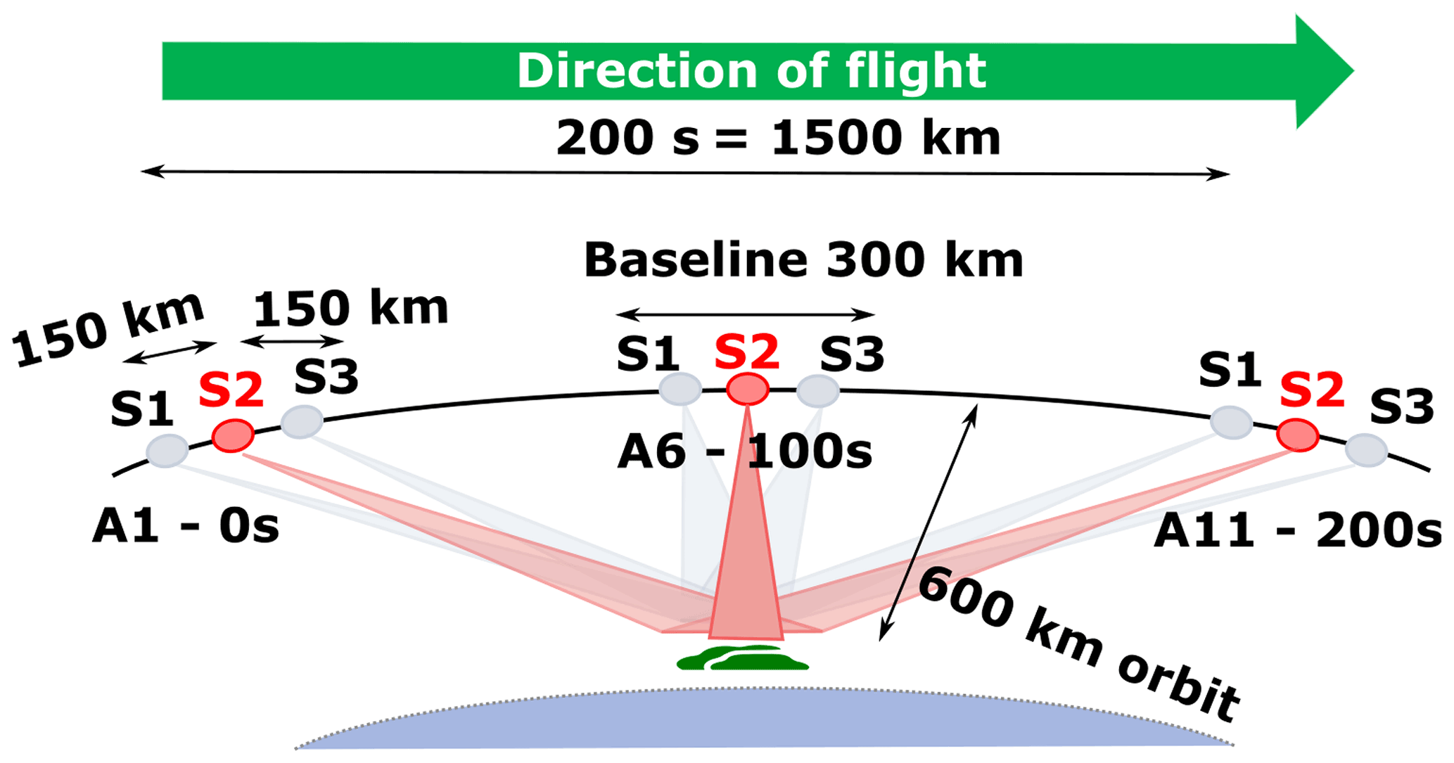
Figure 1CLOUD (C3IEL) observational strategy: multi-view and simultaneous imaging from satellites flying at an altitude of 600 km. Instantaneous (not continuous) stereoscopic pairs or triplets captured every 20 s over 200 s – that is 11 acquisitions (A1–A11). Acquisitions A1, A6, and A11 occur at time t=0, 100, and 200 s, respectively.
The CLOUD cameras, which are the focus of this work, will simultaneously observe the same pixel area under different view angles. Figure 2 shows simulations of some of the successive CLOUD observations corresponding to acquisitions A1 (far from nadir), A6 (close to nadir), and A11 (far form nadir and on the diametrically opposite view to A1 with respect to nadir). The distance between satellites, referred to as baseline B, will be about 150 km.
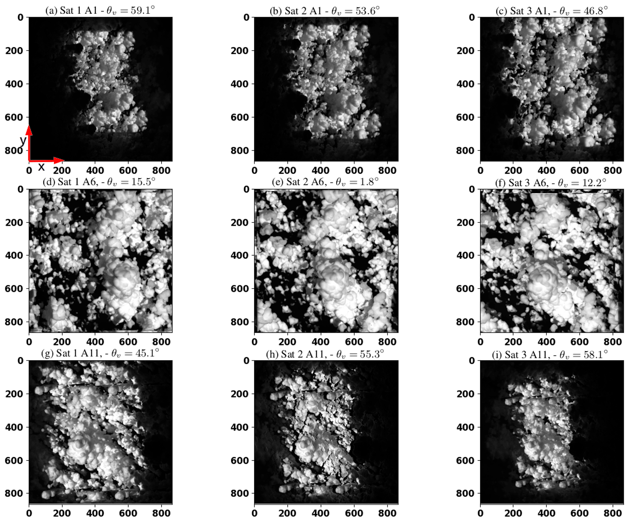
Figure 2Realistic CLOUD (C3IEL) radiance simulations of a deep convective cloud corresponding to A1 (a, b, c), A6 (d, e, f), and A11 (g, h, i); θv is the angular distance of the camera centre from nadir. The sun, at an incidence angle equal to θs=13.6∘, illuminates from the right-hand side of the images. The along and across track directions are identified by the x and y arrows, respectively.
The CLOUD cameras will image a footprint area of about 80 km × 45 km (notice that Fig. 2 shows an area of 15 km × 15 km), with the aim of obtaining an accuracy of the order of a few m s−1 in terms of vertical development speed. The operative wavelength will be 670 nm, where cloud contrast is larger, with molecular and aerosol effects as well as surface brightness being less important. It should be noticed that the satellites are moving from north to south (see x arrow in Fig. 2), and while the across track resolution remains almost constant, the along track resolution decreases for tilted views. This is due to the increase of the footprint in the along track direction and the consequent increase of the ground sampling distance (GSD). Finally, there are image artifacts, mostly towards the periphery of the images and especially visible in the close-to-nadir view (A6) and the off-nadir acquisition (A11), which are associated with the cyclic replication of the cloud field via the Monte-Carlo code. The calculations presented in this paper, namely those corresponding to Figs. 8, 9b, 11a, and 12, were obtained using acquisitions A5 and A6. For such calculations, the region of interest (ROI) used for stereo processing corresponds to the central part of the images (see input images in Fig. 8 – step 1 and Fig. 11a – step 1). Although some artifacts, due to the cyclic conditions of the Monte-Carlo simulations, are visible, they do not affect the results obtained in any way.
The end-to-end simulator: methodology
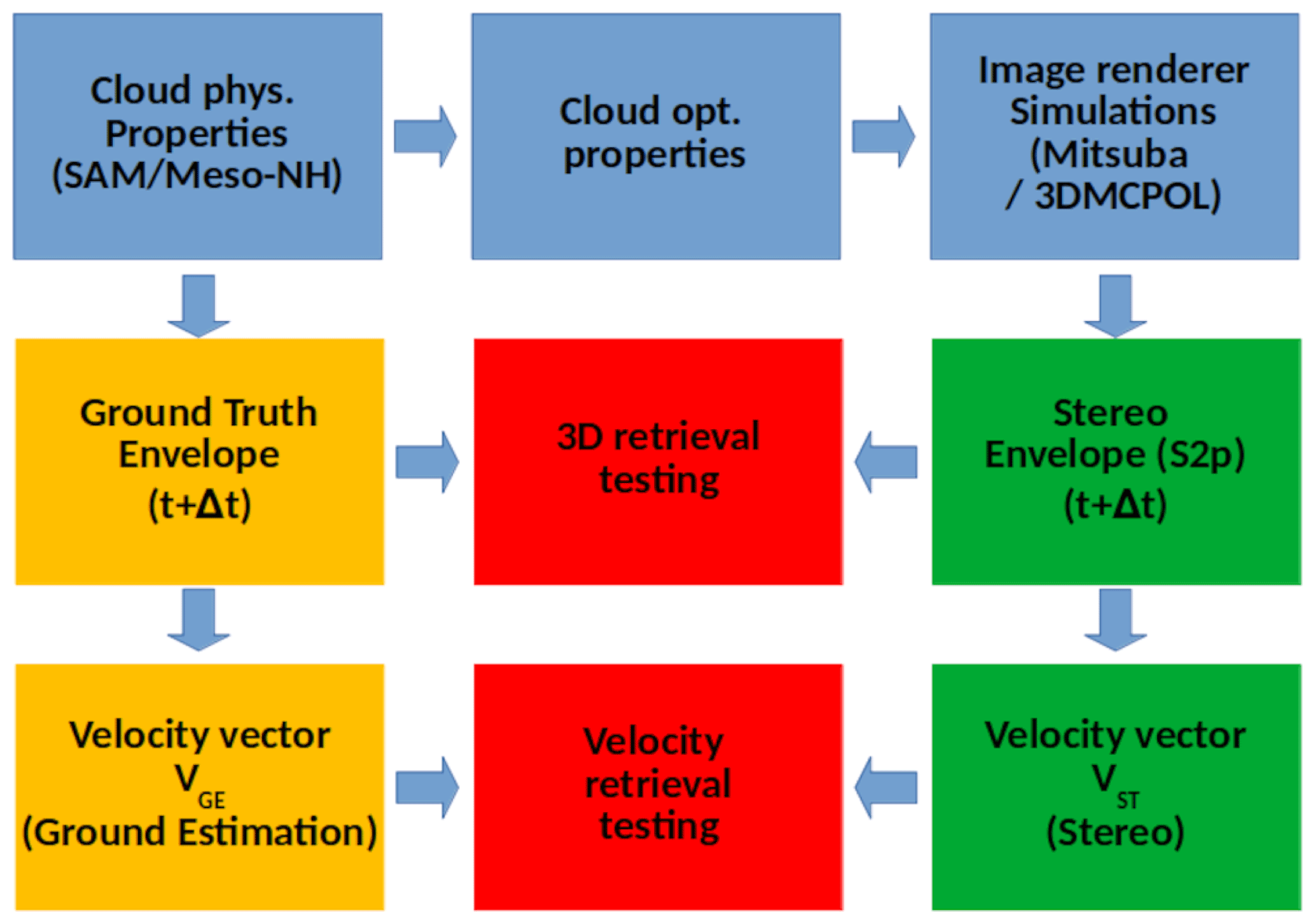
In order to carry out this work while no real C3IEL data yet exist, we had to rely on simulations. A flow diagram of the methodology used (the end-to-end CLOUD simulator) for the retrieval of cloud development velocity is given in Fig. 3. The physical parameters (from the MESO-NH model for the deep convective case and from the System For Atmospheric Modelling (SAM) for the cumulus case) were converted into optical properties, which are then fed to the radiative transfer model 3DMCPOL (Cornet et al., 2010) for the deep convective case and to the image renderer Mitsuba for the cumulus case (Wenzel, 2010) for radiance rendering. Simulations were obtained for perspective projection cameras. The geometry of the external cloud envelope (stereo, ST, cloud) is retrieved for each acquisition from image pairs or triplets and tested against the GT cloud envelope, to which we will refer to as ground truth (GT) cloud envelope, obtained from the cloud physical properties (extinction coefficient or liquid water content) input to the radiance renderers. From these synthetic observations, corresponding cloud pixels, matching cloud features that we refer to as tie points, were tracked between acquisitions; then 3D reconstruction of the cloud envelope was used to map image coordinates to space coordinates for all tie points. In this way, the between-acquisition mean cloud velocity vector (ST velocity vector) was obtained by dividing the distance travelled by the inter acquisition time (20 s). The velocity retrieval was done only for the deep convective case and was, analogously to the geometry retrieval, tested against a ground estimation of cloud velocity (GE velocity vector). The latter was derived from the GT cloud envelopes and independently from the stereo retrieval.
As no real data are available, in order to develop and test the cloud envelope and cloud development velocity retrievals, we simulate C3IEL observations for two test cases ( images for each case). The first case is a cumulus case generated via the atmospheric research model SAM and the image renderer code Mitsuba. The second test case, a deep convective cloud, was simulated via the atmospheric research model Meso-NH and the radiative transfer model 3DMCPOL. The latter allows for the exploitation of more realistic phase functions and was coupled with the outputs of an orbit, attitude, and camera simulator. This second simulation is thus more realistic than the first one and, in the future, will allow one to account for image distortion and satellite orientation error. However, time constraints associated with the high computational cost of the 3DMCPOL runs did not allow the re-simulation of the cumulus cloud.
3.1 Test case 1: the trade wind cumulus
3.1.1 Physical and optical properties
In this section, we turn to the cumulus cloud case generated via the System for Atmospheric Modelling (SAM), a non-hydrostatic anelastic model that simulates cloudy atmospheres in a wide range of scales, from boundary-layer turbulence to hurricanes. It can be configured as an LES model to investigate cloudy or cloud-free boundary layers or as a cloud-resolving model (CRM) to study deep convective clouds and meso-scale cloud systems. The SAM has been successfully ported to many different computing platforms, including massively parallel supercomputers. The original version of the model is discussed by Khairoutdinov and Randall (2003). The CRM that represents subgrid processes in the CSU (Colorado State University) multi-scale modelling framework (MMF) has a relatively simple representation of cloud microphysics. This scheme is fast, but it does not allow for the explicit representation of the freezing or melting of hydrometeors, size sorting of falling precipitation, and aerosol effects on clouds (also known as aerosol indirect effects). Phases of condensed water are diagnosed from the temperature. The physical parameters obtained via SAM for the trade wind cumulus fields are the liquid water path (LWP), the particle number concentration (NC), the wind velocities, the particle effective radius, and the liquid water content (LWC). The cloud field domain consists of voxels, each with size m3. The vertical section of water content (see Fig. 4a) and the relatively low winds (see Fig. 4b and c) of up to 10 m s−1 were plotted for a horizontal resolution of 20 m. With a cloud base between 1 and 2 km, this test case is an example of cumulus cloud that is not well developed, as is often found at mid-latitudes. For the liquid phase, which is the only cloud phase taken into account in this case, the optical properties were quantified from the liquid water content and the effective radius using the Mie theory of scattering. Extinction coefficient σliq and the phase function (PF) were then fed into the rendering code Mitsuba (Wenzel, 2010) to obtain the cloud radiance. In comparison to the deep convective case, we notice vertical winds and COT values (see Fig. 4g) up to 4 and 7 times lower, respectively.
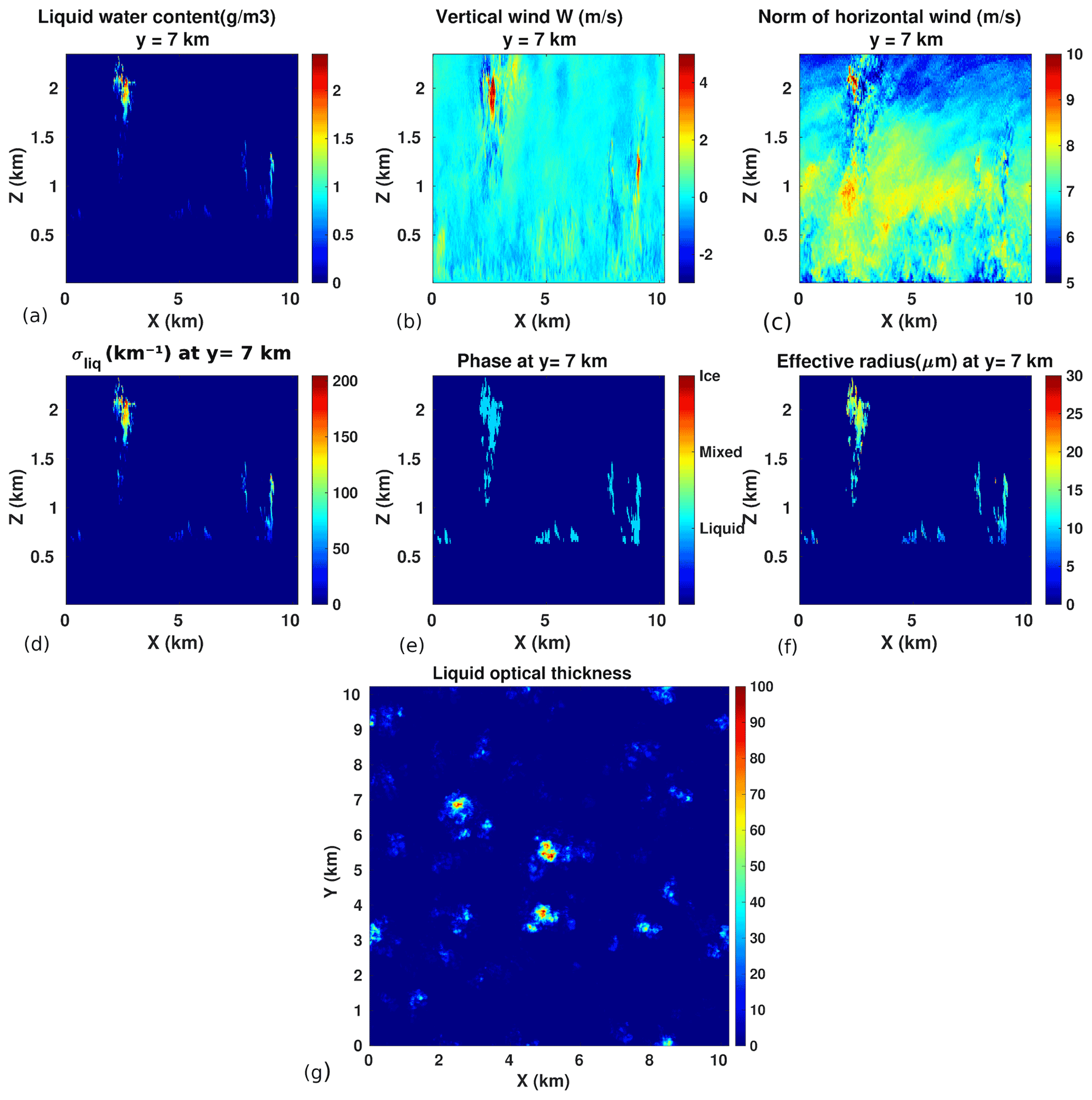
Figure 4Trade wind cumulus physical properties. (a, b, c) Vertical section for y=7 km, from left: liquid water content, vertical, and horizontal wind components, respectively. (d, e, f) Vertical section (y=7 km), from left: liquid extinction coefficient, cloud phase, and effective radius. Panel (g): cloud liquid optical thickness.
3.1.2 The rendering code: Mitsuba
The Mitsuba rendering code enables the simulation of radiance, as observed from a perspective camera. Similarly to 3DMCPOL, Mitsuba implements 3D Monte-Carlo calculations. However, Mitsuba back-propagates radiance from each camera to the sun. Mitsuba is a relatively fast rendering software. However, it is not based on physical first principles that can be derived for an atmospheric medium. This affects the radiometric reliability of the images. However, this effect is not significant in the context of 3D geometric surface reconstruction and tracking of feature points. Here are the assumptions that underlie Mitsuba and our use of it:
-
Only one particle type exists in the medium: a cloud droplet. Hence, the effects of scattering by molecules and aerosols are not accounted for. This is tolerable in our context, because the system is planned to image clouds around optical wavelength of 670 nm. At this wavelength, the effect of molecules and aerosols on space-borne images is small.
-
The angular distribution of scattering is set by the PF. The PF can be derived from physical first principles using Mie theory and the droplet size distribution. The size distribution has some parameters, including the effective radius reff, which vary across the domain. In contrast, Mitsuba assumes a single particle type, a spatially invariant reff, and a Henyey–Greenstein PF. This is a discrepancy from physics. However, this discrepancy is moderated by multiple scattering, which is dominant in clouds. We use a value of 0.85 for the Henyey–Greenstein anisotropy parameter (Mayer, 2009). We use reff and LWC, as provided by the SAM, (see Sect. 3.2.1). The liquid extinction coefficient, σliq (km−1) is calculated via Eq. (2).
-
We simulate clouds over the ocean in the red spectrum. So, we set the ground albedo to 0.
Simulations were obtained for a constellation of three satellites orbiting at an altitude of about 600 km, separated by a distance of 150 km, and imaging the same ground footprint of about 10.24×10.24 km2. The sun is at 22.5∘ from zenith, and the three satellites carry the same camera, with a field of view of 1∘ (field of view in x and y directions are the same). The domain size along the vertical (z) is 4 km. The sensor size is 500×500 pixels for a pixel footprint at the ground of approximately 20×20 m2. Each pixel radiance is simulated using 4 096 photons. In order to test the algorithm for the retrieval of cloud geometry, 11 simulations, obtained every 20 s over a time range of 200 s, were used. Some of them, namely those obtained at a large distance from nadir (t=0 s, 200 s) and those closer to nadir (t=100 s), are shown in Fig. 5. Satellites travel north–south on a linear orbit, and the same considerations about across and along track resolutions for tilted views, seen for the deep convective case, still stand. In Fig. 5, notice the bright cloud tops and shaded cloud sides. In the dark-shaded regions, feature identification is more difficult.
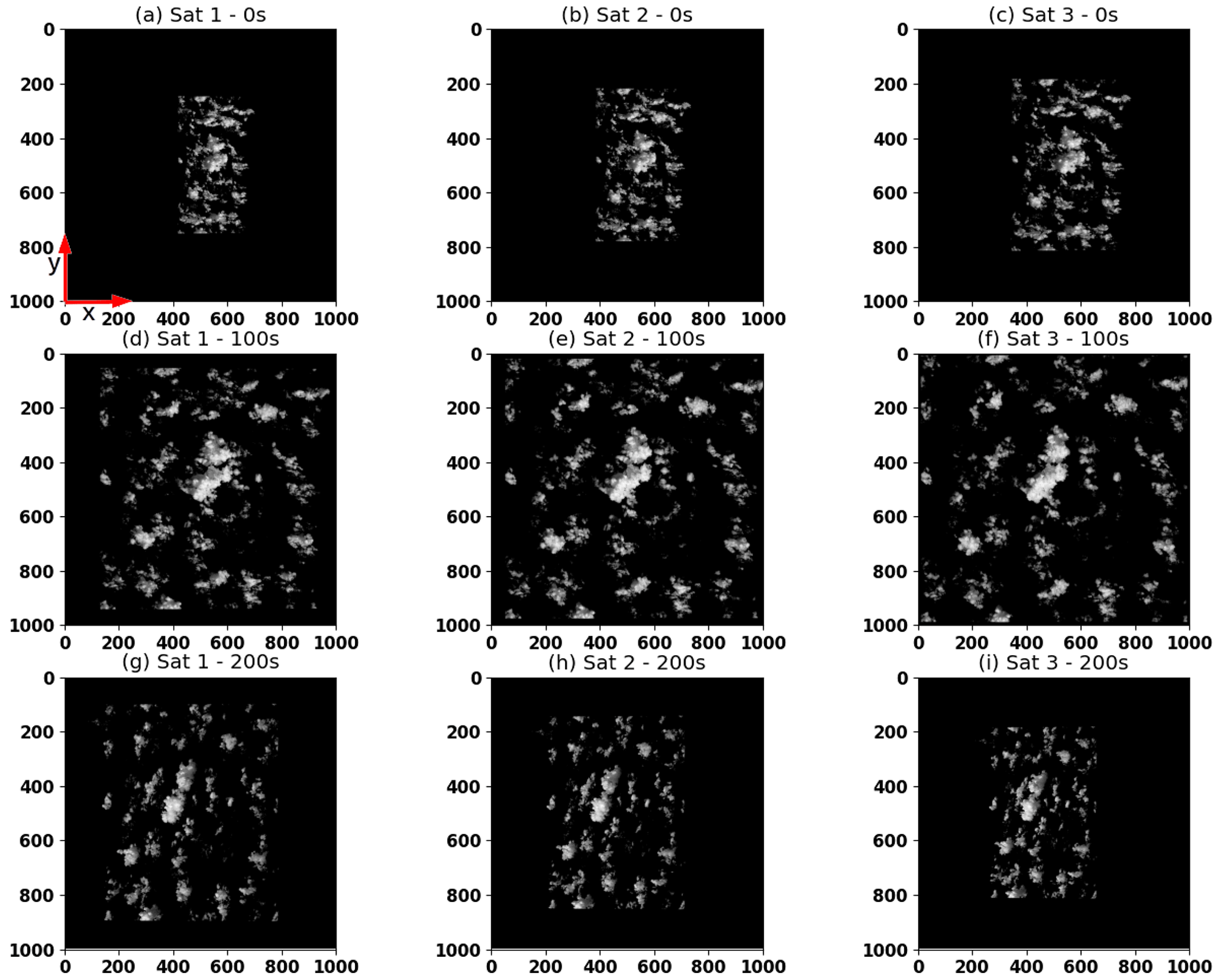
Figure 5Realistic CLOUD (C3IEL) radiance simulations for a cumulus cloud case and corresponding to acquisitions A1, A6, and A11. The along and across track directions are identified by the x and y arrows, respectively.
3.2 Test case 2: a deep convective cloud
3.2.1 Physical properties from LES
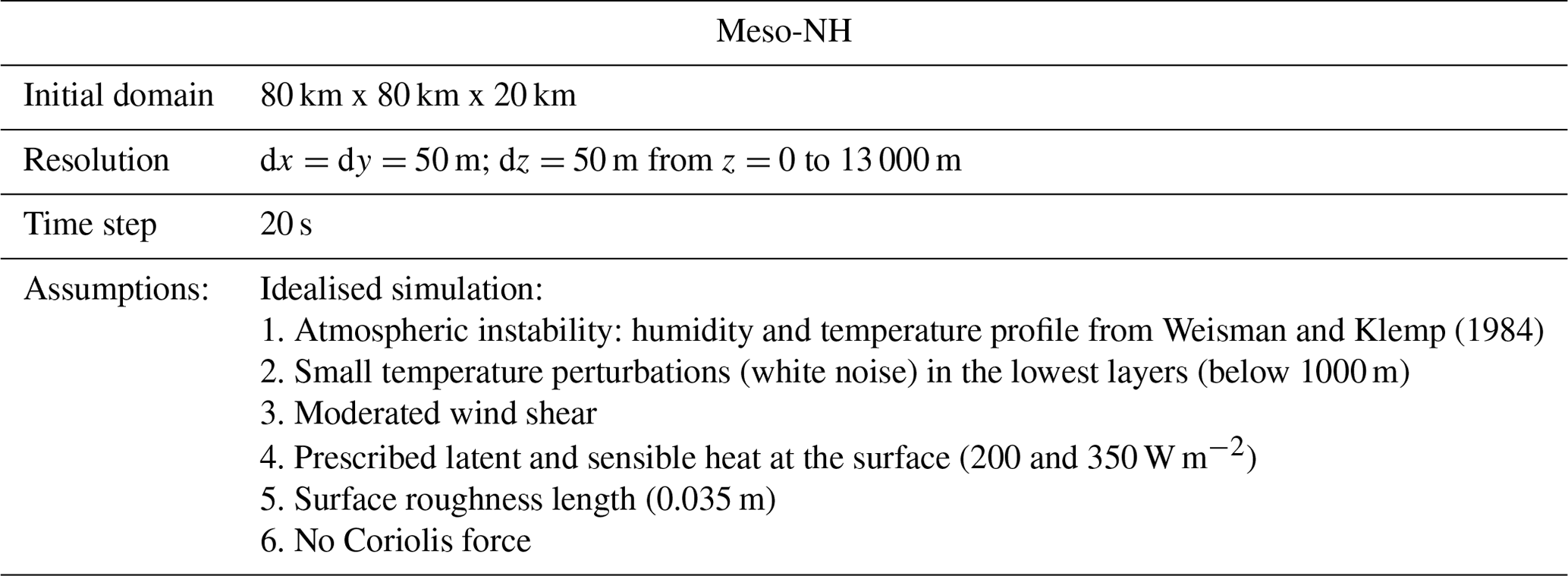
The second test case is a deep convective cloud simulated with the non-hydrostatic mesoscale atmospheric model Meso-NH model (Lac et al., 2018), used in LES mode. Figure 6 shows the vertical section, at 22 km (6 km from the origin of the y axis located at 16 km, see Fig. 6g and h), of total water content as well as vertical and horizontal wind components. Simulations were done (Strauss et al., 2019) with a 3D turbulence scheme (Cuxart et al., 2000), the microphysical scheme ICE3, including five hydrometeor species (Pinty and Jabouille, 1998), and no radiation scheme. Cloud model domain, resolution, and assumptions are given in Table 1. The spatial resolution of the domain is 50 m. As the entire cloud scene ( cells) is too large to be handled by 3DMCPOL, sub-domains of cloud cells were extracted from the initial scene. With a horizontal extent of around 10 km and a cloud top at about 9 km, this is a case of well-developed convective cloud characterised by relatively strong in-cloud air stream speeds of up to 20 m s−1 for both horizontal and vertical components. Consistently, relatively large values of water vapour mixing ratio (not shown), up to kg kg−1, are observed up to 2 km from the ground.
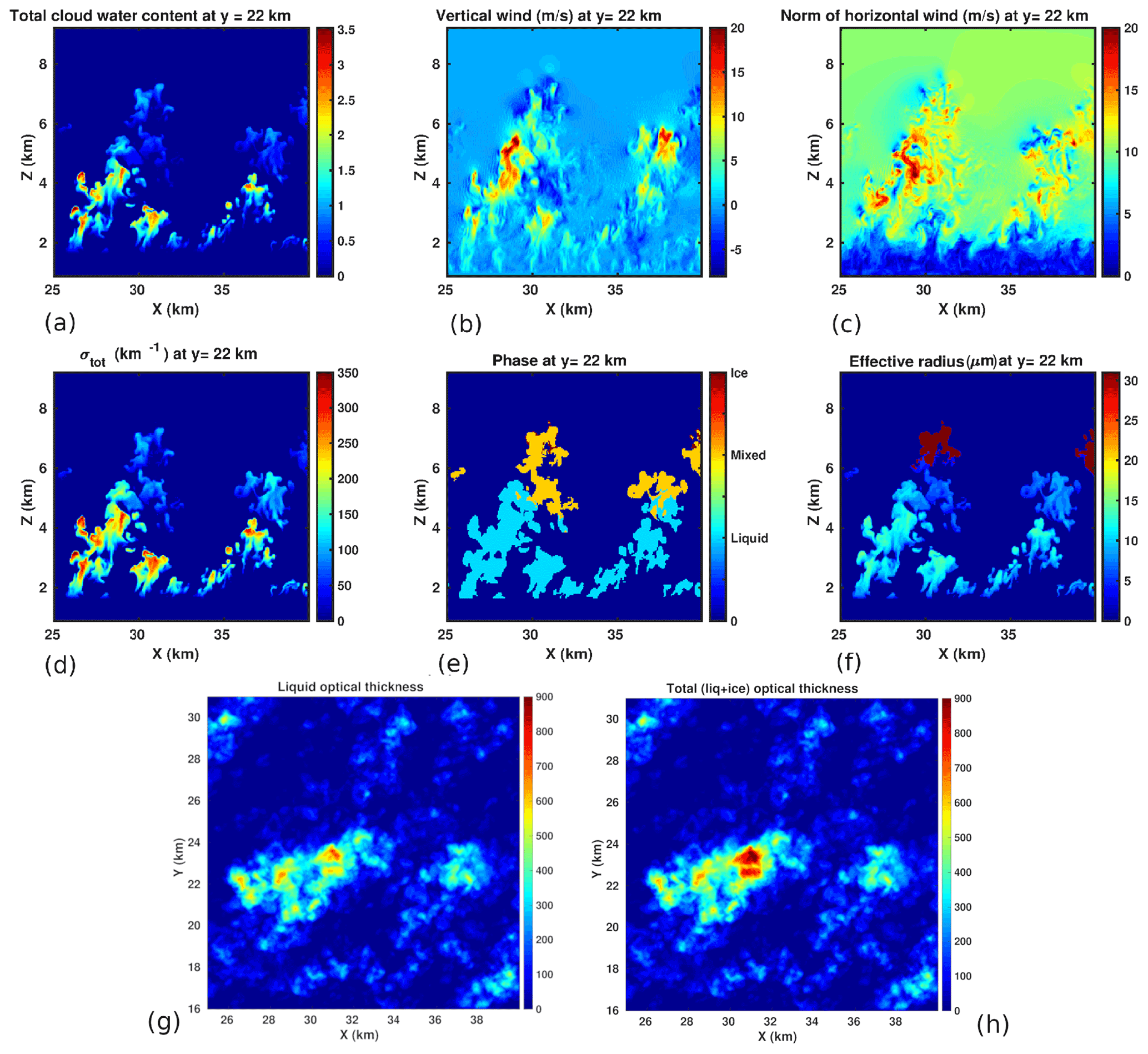
Figure 6Deep convective cumulus physical properties. (a, b, c) Vertical section (y=22 km, that is 6 km from the origin of the y axis located at 16 km) of cloud total water content as well as vertical and horizontal wind components, respectively. (d, e, f) Vertical section (y=22 km) of total extinction coefficient, cloud phase, and effective radius, respectively. Value of 31 (dark red) is associated with voxels where the mean ice phase function is used. (g, h) Liquid optical thickness and total optical thickness (liquid + ice), respectively.
Table 1Settings of Meso-NH for the simulations of the deep convective cloud.
3.2.2 From physical to optical properties
Cloud optical properties – such as extinction coefficient, single scattering albedo, and phase function (PF) – have to be fed into the 3DMCPOL in order to compute cloud radiances. For the liquid phase, they are quantified from the water content and effective radius using the Mie theory of scattering. As the version of the Meso-NH model used here does not compute the particle size distribution (PSD), we find the effective radius of the water droplets by using Eq. (1) (Martin et al., 1994):
where rl is the mass of liquid water per unit volume of air, ρ is density of water, and k is a constant – 0.8 or 0.67, for the maritime or continental scenario, respectively. The droplet number per unit volume N is set to 300 cm−3. Equation (1) was established for stratocumulus clouds, and although not completely appropriate for deep convective clouds, it reproduces the observed values fairly well (Freud and Rosenfeld, 2012). Furthermore, this is not going to affect the assessment of the stereo retrieval in any way. The liquid extinction coefficient, σliq (km−1), is calculated using Eq. (2):
For the ice part, the Baran's parameterisation (Baran et al., 2014) is used to compute extinction coefficient, ice single scattering albedo ωice, and PF from the ice water content and ice temperature. In this case, the extinction coefficient is obtained from look-up tables of absorption and scattering coefficients. A modified Henyey–Greenstein phase function (Baran et al., 2001) is then computed from the asymmetry parameter g, and the average ice phase function is taken. For the mixed phase, the extinction coefficient is the sum of the liquid and ice extinction coefficient, while the single scattering albedo ωmix is taken as the average of ωice and ωliq weighted by the respective extinction coefficient. The cloud phase associated with the larger extinction coefficient (ice vs. liquid) is selected. As a result, the vertical section of total extinction σtot, cloud phase, and reff are plotted in Fig. 6d, e, f. Relatively large values of σtot up to 300 km−1 are observed between 3 and 4 km, where mostly liquid particles are found, as well as significantly lower values of σtot above 4.5 km, where the transition from liquid to mixed phase occurs; also, noticeably, the position of the peak of the particle size distribution varies with altitude, with larger ice crystals above 6 km and smaller cloud particles below. Liquid and total optical thickness τliq and τtot (see Fig. 6g and h), obtained by integrating σliq and σtot respectively, over the geometric extent of the cloud, have also been plotted. Noticeable are the very high cloud optical thickness (COT) values of up to 700, typical of this type of cloud.
3.2.3 The radiative transfer: 3DMCPOL
Shadowing and illumination effects are of great importance when it comes to detecting identical cloud features from pairs or triplets of CLOUD images. That is why clouds cannot be assumed to be plane-parallel and homogeneous when computing radiances. Moreover, the high resolution of the CLOUD cameras makes the independent pixel approximation no longer valid. In order to account for these effects, a radiative transfer model allowing calculations in a 3D atmosphere is necessary. With the aim of obtaining realistic observations of the CLOUD sequence of acquisitions, we use the forward 3D Monte-Carlo radiative transfer model (Cornet et al., 2010). 3DMCPOL was initially devised for computing radiances in an orthographic mode that has parallel output directions for the radiance of each camera pixel. As the satellite can be considered to be at infinity, this assumption is valid for the simulation of a small part of a large swath or when 3D radiative transfer is used to simulate sub-pixel heterogeneity (Cornet et al., 2018). However, to render a large portion of the images at a high spatial resolution in camera mode, the orthographic assumption is no more valid. Furthermore, pixel size increases with the distance from the image centre, and so does the footprint for tilted views. To account for this particular geometry, 3DMCPOL uses the output of an orbit, attitude, and camera simulator developed by CNES and dedicated to the C3IEL mission. This simulator is coupled with CNES geometric library (Euclidium) in order to obtain grids at different altitudes, giving the correspondence between a 3D position in the medium to the index (i,j) of the camera image and to the output direction defined by a zenithal and azimuthal angles. From these grids, trilinear interpolation gives access to the image pixel line and column and to the line of sight in order to apply the local estimate method used in 3DMCPOL. Sampling of the grids is managed so that the trilinear interpolation does not bias the samples within 0.1-pixel accuracy. In this way, the sphericity of the orbit and the orientation of the satellites are accounted for. In this work, satellite position and orientation are assumed to be known exactly. However, this is not true, and the corresponding errors are expected to deteriorate the results presented here. We will be able to test such a statement in the future – once these sources of error will have been modelled for each camera – by exploiting the combined use of Euclidium and 3DMCPOL. Another advantage of the simulator is the possibility of including image distortion. Due to computational limitations, we were not able to compute the entire field of view of the cameras, which is 80 km × 45 km, composed of 4608×2592 pixels, with a size of 17 m at nadir. Consequently, the input cloud was chosen to be a 3D medium, with voxels and with 50 m resolution in the three directions, corresponding to a horizontal extent of the cloudy medium of 15 km × 15 km. Figure 2 shows 3DMCPOL simulations for the acquisition A1 (T0) off nadir (top three figures), acquisition A6 (T0+100 s) (middle images – approximately at nadir), and acquisition A11 (T0+200 s) off nadir but on the diametrically opposite view to A1 with respect to nadir (bottom figures), respectively. Each simulation is identified by satellite and acquisition numbers .
3.3 The ground truth point cloud
To test the stereo algorithm as a function of the geometry and the number of satellites, the ground truth (GT) point cloud was derived from the LWC, issued from the physical models, for both cloud cases. The GT point cloud is defined for each direction x, y, and z as the boundary cloud voxels corresponding to the cloud contour and was determined for all cross sections parallel to the xy, yz, and xz planes and for each cloud cell. As for testing of the stereo cloud (ST cloud) against the GT cloud, covered in Sect. 4, the GT cloud was mapped from East-North-Up (ENU) to UTM (Universal Transverse Mercator) coordinates. The GT point cloud so obtained is shown in Fig. 7 for the deep convective case and for the trade wind cumulus – Fig. 7a and b, respectively. For simplicity, in what follows, we will refer to it as the GT cloud or GTAN (AN= acquisition number) when the acquisition number is specified.

Figure 73D cloud envelope referred to as GT (ground truth) point clouds. Point colour shows the Z coordinate (altitude from ground expressed in m).
In this section, we first discuss the stereo retrieval of cloud geometry – in other words, the 3D space retrieval of the cloud pixels sensed by the cameras – then the method applied for testing the retrieval, and eventually the results of the testing in Sect. 4.2.
4.1 The 3D reconstruction: dense matching and triangulation
For each acquisition of synthetic pairs or triplets, retrieval of the cloud envelope (ST cloud) is performed. On general grounds, for each image point, the corresponding scene point depth (i.e. distance from the camera) is determined by first finding matching pixels (i.e. pixels showing the same scene point) in the other image(s) and then applying triangulation to the found matches to determine their depth. The retrieval was done by means of the stereo reconstruction algorithm s2p (satellite stereo pipeline) (de Franchis et al., 2014). The use of this algorithm requires knowledge of the analytical camera models that are inverse (see Eqs. 3 and 4) and direct (see Eqs. 7 and 8) projection models of the camera mapping from geographical coordinates (lat, long, height) to image coordinates (r, c) and vice versa, respectively. Such models are expressed as the ratio of polynomials of degree Nth, whose coefficients, the RPCs (rational polynomial coefficients), are fit to the mapping of the physical camera model for each camera and each orientation. Such calculations were done for polynomials of degree 3 () according to the procedure described by Tao and Hu (2001) for the cumulus case and via the Euclidium library for the deep convective case.
The s2p process pipeline can be summarised as follows: input images are first cut into tiles, where the cameras are assumed to be affine (i.e. perspective projection). With respect to the calculations presented in this work, we use a tile size equal to the ROI (865 pixels × 865 pixels), as we achieve satisfactory rectification with no need of further reduction of the tiling. With regard to Fig. 8, the input reference (ref) and secondary images (sec) are first rectified (rect ref, rect sec). Stereo rectification allows for the restriction of the search for corresponding features from the entire image to a single line. For any point p in the reference view, the corresponding point p′ in the secondary image, provided that it exists, lies on the epipolar line of p, that is EL p. Analogously, p lies on the epipolar line of p′, EL p′. There is a correspondence between the epipolar lines of the two views for images taken with pinhole cameras. In this case, the epipolar lines are said to be conjugate. The purpose of rectification is that of resampling the images in such a way that matching points are located on the same row (epipolar lines become horizontal), thus simplifying the search of matching features and allowing one to use conventional stereo matching algorithms. Rectification consists in projecting the input images onto a common grid, given a reference altitude, such that the epipolar direction is line-wise. Consequently, any point having a different altitude than the reference altitude will experience a disparity in line direction. Rectified and reference images are linked via the homography transforms H1 and H2; s2p calculates the homographies by exploiting the RPC camera models. The stereo-rectified images are fed to the stereo matching algorithm to find all pairs of matching cloud features (i.e. image points (h,k) and , dx and dy being the disparities along x and y, oriented as the red arrows in Fig. 8 show, with dy=0 being the epipolar lines horizontal). The latter are linked by horizontal yellow lines (see Fig. 8, top right). The block-matching algorithm that we use, more global matching (MGM) (Facciolo et al., 2015), was selected among those available (semi-global block matching – SGBM; multi-scale multi-window stereo matching – MSMW – Buades and Facciolo, 2015; and so forth) as one of the top-ranked stereo vision algorithms. MGM looks for the disparity map that minimises an energy cost function. The disparity dx associated with each pair of matching features is the distance between two corresponding points in the rectified images (see Fig. 8, step 3, dx= rect sec x− rect ref x). Cloud pixels closer to the cameras (i.e. cloud top) are associated with negative disparity values (deep blue points), as for any given pair of matching features, rect sec x< rect ref x, whereas for points farther away from the cameras, associated with positive disparity, rect sec x> rect ref x (orange and red pixels). Each pair of tie points is mapped back in the original images by homography inversion (see Eqs. 5 and 6).
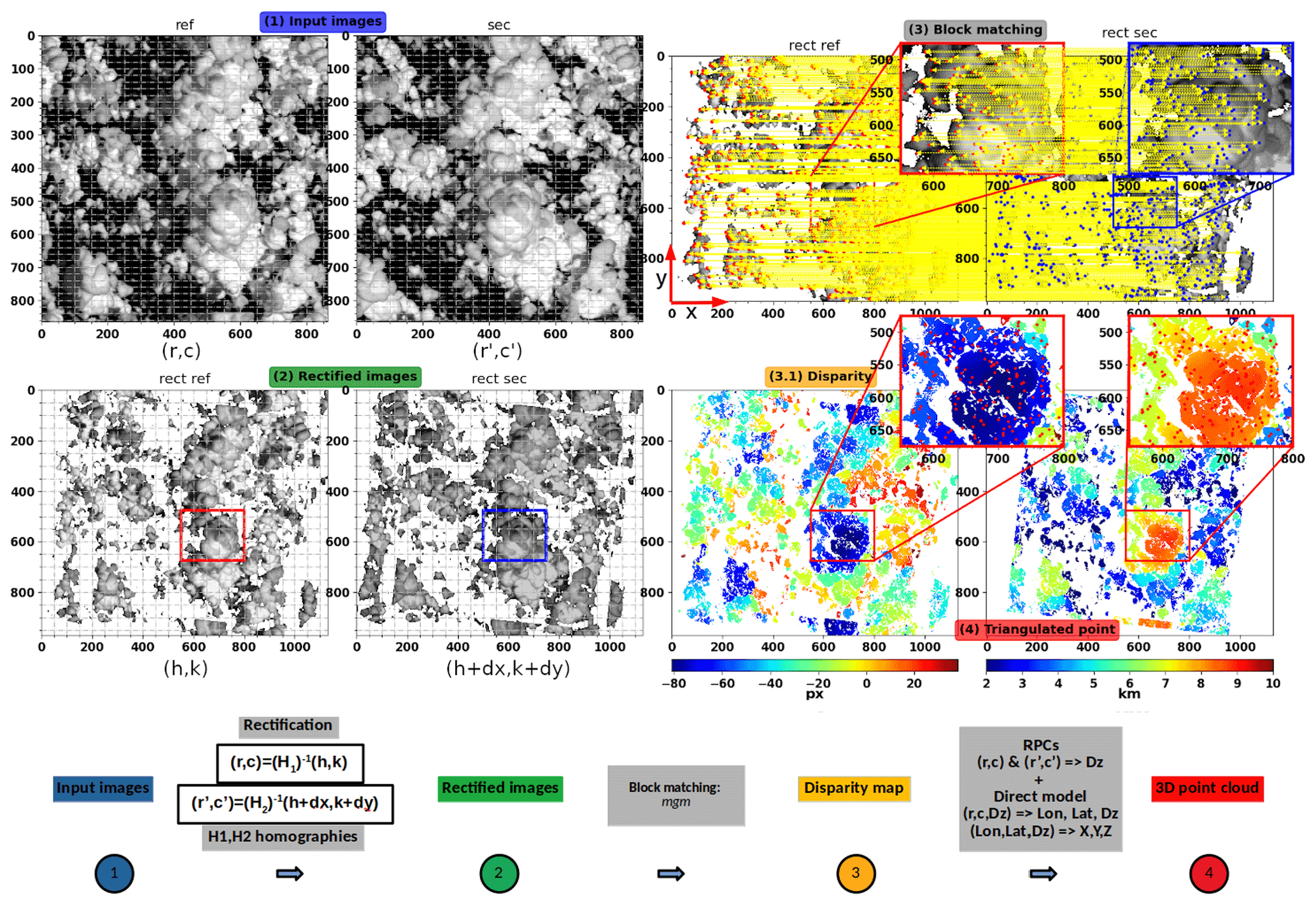
Figure 8Step-by-step 3D reconstruction via s2p algorithm. Top left: reference and secondary images (ref, sec). Notice that ref and sec have been rotated 90∘ clockwise for consistency, with the orientation of the along track direction x. Bottom left: (2) rectified images (rect ref, rect sec). Top right: (3) tie points from block matching; (3.1) disparity map; (4) 3D reconstructed point cloud (z – altitude from ground). These calculations were obtained using acquisition A5.
The height of a point from ground HG, given its location inside two images ((r,c) and ), is calculated iteratively via RPCs; and are mapped into geographic coordinates (lat, long, HG) via the inverse RPCs model – Eqs. (7) and (8) – and then are turned into UTM X, Y, Z coordinates. As a result, a point cloud is generated. An array of shape [h,w] (h and w being image height and width in pixels of the rectified reference image), where each pixel contains the UTM X, Y, and Z coordinates of the triangulated point, is obtained (see triangulated Z in Fig. 8, step 4). Moreover, s2p associates to each retrieved point the colour coordinates [R, G, B] of the corresponding pixel from rect ref (grey scale). A radiance threshold (about 2 % of the maximum radiance) is used for filtering deep, dark points where no cloud pixels are present. This array of spatial and colour coordinates is what we refer to as the ST point cloud.
The stereo retrieval from triplets that we discuss in this paragraph works by pairs. Given a set of three images, let us assume Image 2 is our reference image. Tie points are first searched between pair (1, 2) and then between pair (2, 3). The corresponding disparity maps (one for pair (1, 2) and one for pair (2, 3)) are transformed into height maps (distance from ground), which were calculated on the grid of the original reference image. For a given tie point, we then have two values of HG: HG1 from pair (1, 2) and HG2 from pair (2, 3), respectively. The mean of HG1 and HG2 is taken if (HG2−HG1) is less than a fusion threshold (user chosen), otherwise the point is discarded. From this point, the 3D retrieval from triplets goes on exactly as we have seen for two images: rn, cn, and HG are mapped to lat, long, HG, and eventually into UTM X, Y, Z.
One of the main questions in preparation for the mission concerns the choice of the baseline and whether retrieval from triplets, in comparison to retrieval from pairs, is significantly more accurate and if it leads to a larger number of retrieved points. The number of detected points was plotted as a function of the acquisition number for two and three satellites for the cumulus case (see Fig. 10a). This was done for a baseline B of 150 km (Sats 1–2 and Sats 2–3) and 300 km (Sats 1–3) and for three satellites (Sats 1–2–3) with a fusion threshold of 30 m. The latter was chosen after having ascertained that alternative values brought no significant difference in terms of retrieval. We clearly see that the number of detected points decreases with the distance from nadir (A5–A6) because of the decreasing resolution for tilted views. Concerning the distance between the satellites, the number of detected points is higher for satellites separated by 150 km (Sat 1–2 or Sat 2–3) than for satellites separated by 300 km (Sat 1–3), as the matching features are easier to identify.
The threshold of 30 m leads to some points being discarded, which appears to reduce the number of detected points slightly, when using three satellites instead of two. It is important to emphasise that the s2p algorithm uses two-view stereo at a time and then merges these independent two-view stereo reconstructions into a single reconstruction. This is contrary to full multi-view stereo methods (e.g. which use the whole set of three-views simultaneously). Multi-view methods are widely used in computer vision due to the advantages they bring over the two-view stereo (Zhang et al., 2019). Using full multi-view stereo methods might lead to different results in terms of 3D reconstruction via three cameras, namely that the 3D cloud envelope retrieval can be more accurate and lead to more detected points compared to when using only two views. However, this must still be confirmed.
4.2 Testing of the stereo retrieval against the ground truth point cloud via M3C2 algorithm
The comparison of two sets of point clouds is not trivial, and several metrics can be used. We chose to use the multiscale model to model cloud comparison (M3C2) algorithm (Lague et al., 2013) to test the stereo retrieval against the GT point cloud. M3C2 is available from the open source project 3D point cloud and mesh processing software CloudCompare (CloudCompare, 2010). M3C2 allows for the computing of signed and robust distances for each point of the reference cloud along the local normal, as represented in the schematic of Fig. 9a. For any given core point i of the reference cloud (S1 in step 1), a normal vector N is defined by fitting a plane to the neighbouring points within a radius from i. A cylinder of cross section d (d being the projection scale) and longitudinal length L, whose main axis goes through i, is then aligned along N in order to intersect S1 and the compared cloud (S2). The intercept of S1 and S2 with the cylinder defines two subsets of points. Projecting each of the subsets on the axis of the cylinder gives two distributions of distance. The mean of the distribution gives the average position of the cloud along the normal direction, i1 and i2. The local distance between the two clouds LM3C2(i) is then given by the distance between i1 and i2. The results discussed in the next section were obtained by assigning a value of 100 m to the normal scale D, d, and L. This was done after having ascertained that no significant difference in the outcome was attained for different values. The output of M3C2 are the absolute value of the distance LM3C2 and the normal components of N. The displacement vector components LM3C2x, LM3C2y, and LM3C2z of the core points are then calculated as the simple product LM3C2=LM3C2N. The ST point cloud (output of s2p) was compared against the GT point cloud, defined in Sect. 3.3. Figure 9b shows the ST (left) and GT (right) clouds for the deep convective case (top line) and the cumulus case (bottom line), respectively. The colour associated with each point is the altitude from ground Z. Also shown is the M3C2 absolute distance (centre) for the deep convective case (top) and the cumulus case (bottom). Both retrievals correspond to acquisition A5 (close-to-nadir view). For both test cases, the number of ST points is quite dense, and most of the detected points match with the GT point cloud.
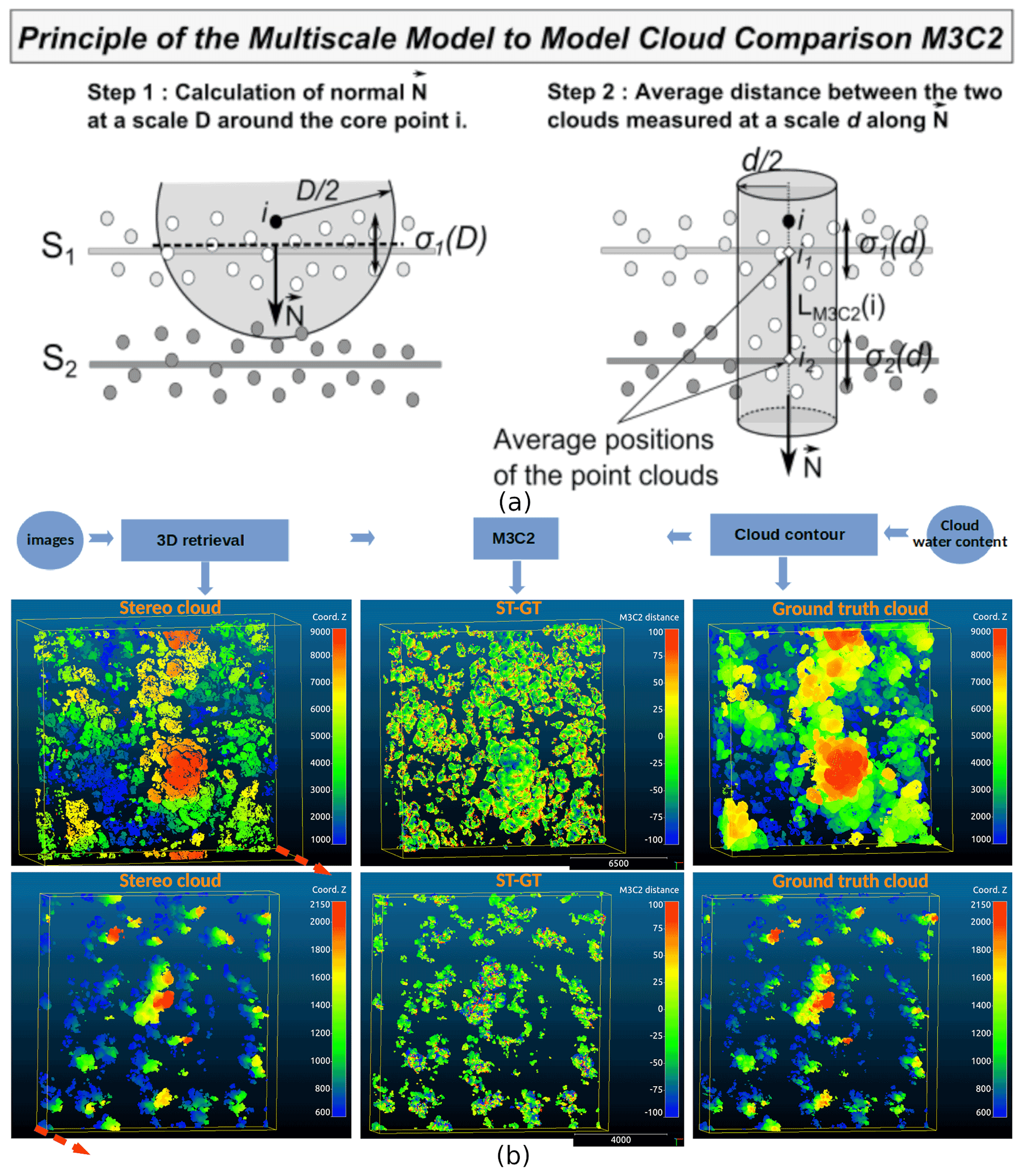
Figure 9(a) Schematic of M3C2 working principle – from Lague et al. (2013). (b) ST (left) and GT (right) point clouds for the deep convective case (top) and the cumulus case (bottom), M3C2 absolute distance in metres (centre) for the deep convective case (top) and the cumulus case (bottom). The red arrow is oriented along the z axis.
To quantify the stereo retrieval error, for any given satellite configuration, we have measured the distance between retrieved and ground truth points using M3C2. For each acquisition and from LM3C2x, LM3C2y, and LM3C2z, we have then calculated the mean difference (bias) and the RMSE along the axes x, y, and z. The three plots in Fig. 10b, d, and f show the mean difference along z, x, and y axis as a function of the acquisition number. The mean difference (its absolute value) along z is less than 25 m, while it is less than about 5 m along x and y. Such values can partly be ascribed to the stereo-opacity bias, associated with low extinction near the cloud top, as discussed by Mitra et al. (2021). The skewed distribution of the error in Fig. 10b for the views A9–A11 may be due to the fact that fewer cloud features are visible, as the clouds are less illuminated by the sun, with larger portions of the cloud field shaded, as can be seen from Fig. 5g, h, and i. The RMSE (see Fig. 10c, e, and g) for the z coordinate is less than 40 m and increases slightly with the distance from nadir. The same increase with the view angle is more evident with RMSEx and RMSEy. Similar results with bias <4 m and RMSE <25 m were obtained for the deep convective cloud case (not shown here). Based on the s2p algorithm, it appears that none of the configurations significantly outperforms the others in terms of retrieval quality. However, as already pointed out at the end of Sect. 4.1, these conclusions may differ if analysis would use alternative 3D reconstruction algorithms based on full multi-view stereo.
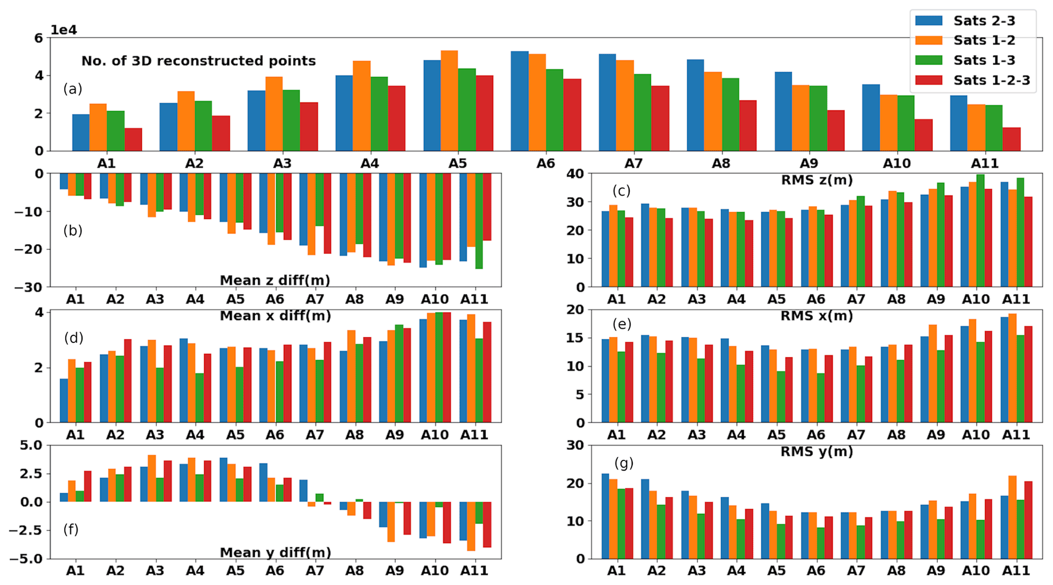
Figure 10Results of the testing of the 3D retrieval for the cumulus case. (a) Number of stereo-retrieved points as a function of the acquisition number (A5, A6 are close to nadir) for two vs. three satellites and for B =150 km (Sats 2–3 and Sats 1–2) and B =300 km (Sats 1–3). (b, d, f) Mean difference between ST and GT point clouds for each acquisition along z, x, y. (c, e, g) Root mean square error (RMSE) of the difference between ST and GT point clouds for each acquisition along z, x, y.
In this section, we look into the velocity retrieval method applied to the ST clouds (Sect. 5.1) and another independent method for deriving a ground estimate of cloud development velocity from the physical model (Sect. 5.2). As the retrieved ST point clouds are not sufficiently dense to be used for the matching of cloud features between two acquisitions, we look for tie points between successive images by exploiting the block matching algorithm of s2p; we then map image points to 3D space points via 3D reconstruction.
5.1 3D cloud development velocity from 3D retrieved cloud envelopes
The working principle of the ST velocity retrieval is illustrated in Fig. 11a. Tie points are first found from a pair of images taken from two consecutive acquisitions via MGM (see Fig. 11a, step 1, ST2A5 – top and ST1A6 – bottom). Red dots, representing the tie points so found, are linked by yellow lines (notice that only a few of them are shown, given the high density of points). Each image from the chosen pair is then utilised with one or two simultaneous images (secondary images in the top right corner) to do the 3D retrieval of the cloud envelopes, as described in Sect. 4.1, for acquisitions A5 and A6, respectively. The tie points from step 1 are then mapped in the rectified images (step 2), and the retrieved UTM X, Y, and Z (step 3) are interpolated (to the nearest point if distance <1 pixel) to the locations identified by the floating tie points (step 4). Ultimately, tie points in image ST2A5 (i5, j5) are mapped to tie points in space (X5, Y5, Z5) for A5; analogously, tie points in image ST1A6 (i6, j6) are mapped to tie points in space (X6, Y6, Z6) for A6. The velocity vector is then derived according to Eq. (9).
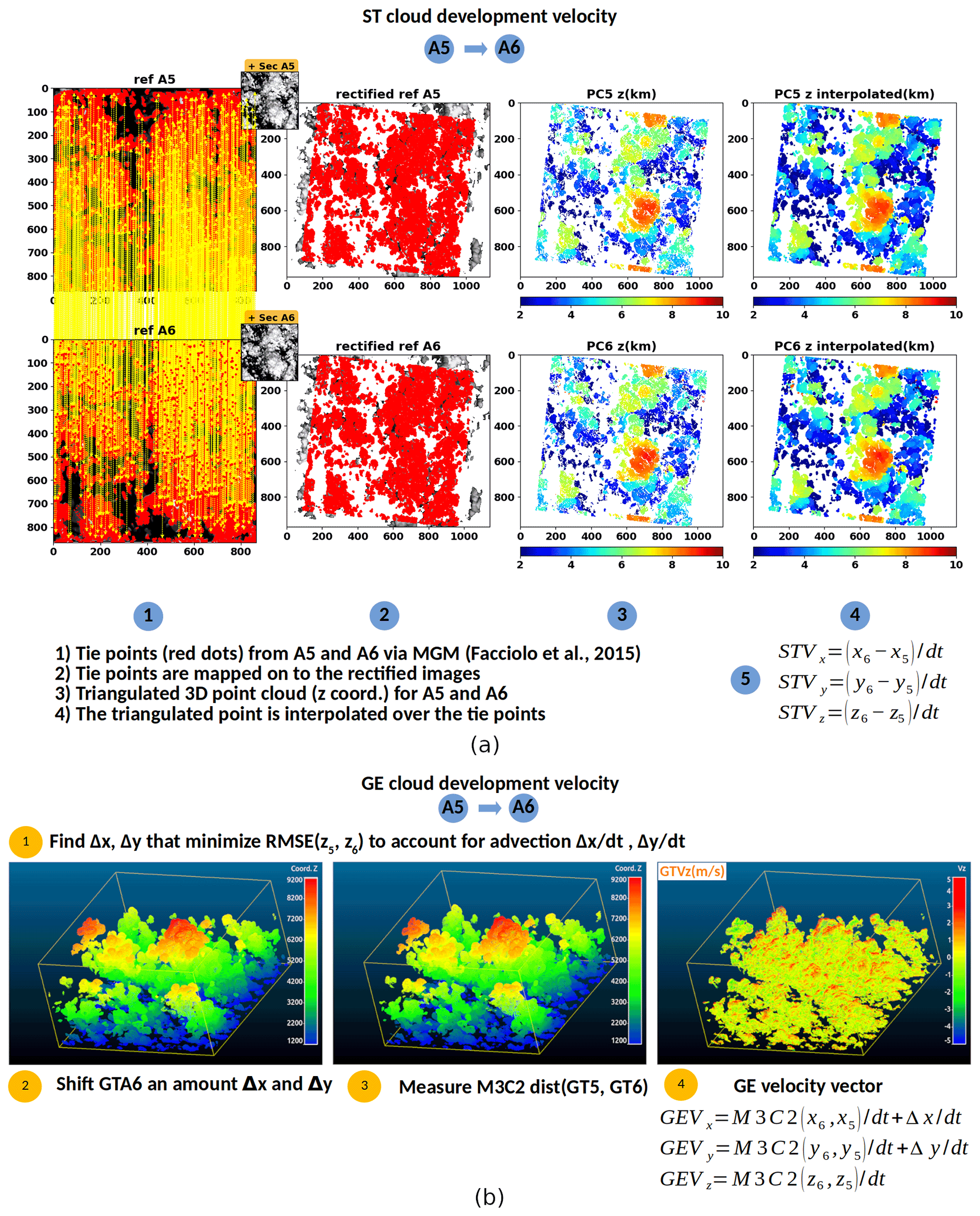
Figure 11Cloud development velocity algorithms. (a) From ST clouds – (1) tie points from images ST2A5 and ST1A6, (2) tie points are mapped on to the rectified images, (3) 3D retrieved point clouds (for A5 and A6), (4) 3D point clouds interpolated to the tie points, (5) mean ST velocity vector. (b) From GT clouds – (1) Δx, Δy that minimise RMSE(z5,z6) are calculated, (2) GTA6 is translated to an amount Δx, Δy to account for advection, (3) M3C2 cloud-to-cloud distance is calculated, (4) the mean GE velocity vector is derived.
The error associated with the velocity retrieval is given by the contribution of the block matching and stereo retrieval errors. MGM mismatch error was quantified in a previous work (see Facciolo et al., 2015) in terms of bad pixel ratio (percentage of pixels with error >1 pixel) and was compared to other state-of-the-art semi-global matching methods, yielding the lowest average errors. In addition to false matches, rounding errors occur when the retrieved X, Y, and Z (given on an integer grid) are interpolated to the floating tie points coordinates. In Sect. 5.3, the retrieved velocity is compared to an estimate of cloud development velocity derived from the GT envelopes, to which we turn next.
5.2 3D cloud development velocity from the GT point clouds: ground estimation (GE)
3D cloud development velocity was derived from the GT point clouds from two consecutive acquisitions. This is further illustrated in Fig. 11b for acquisitions 5 and 6. First, we determine the horizontal displacement that minimises the RMSE(ZA5,ZA6), with Z being the altitude from ground (step 1). This is done to account for the advection, which, for this test case, we assume to be constant, over the extent of the cloud field. We find that the superposition of GTA5 (reference cloud) and GTA6 (secondary cloud) is optimised by shifting GTA6 an amount Δx=130 and Δy=120 m (step 2). Then the M3C2 distance, discussed in Sect. 4.2, is used to measure cloud-to-cloud distance (step 3). As a reminder, this is the distance between two average positions along the local normal, from the reference cloud to the secondary cloud. This distance is decomposed along X, Y, and Z to get the velocity vector after adding the average advection (see Eq. 10) (step 4). The resulting Z component of the velocity GEVz is shown in the right corner of Fig. 11b. It should be specified that, as opposed to the retrieved ST products, this method does not rely on finding matching cloud features. For any given point from the reference cloud, its matching point from the secondary cloud is searched for along the local normal.
In the coming section, we will compare the retrieved cloud velocity to the velocity derived from GE.
5.3 Comparison between the ST velocity and GE velocity
With respect to the following comparison, the velocity of each tie point in 3D space is compared to the velocity of the nearest point extracted from the GT velocity cloud if the distance is less than 100 m. Figure 12a and b show the cloud velocity vectors obtained between A5 and A6 from the ST and GT clouds, respectively. In the top part of each figure, from left to right, each cloud pixel is associated with a colour that represents the value of the velocity along z, x, and y, respectively. The bottom part of each figure shows, instead, the distribution of the cloud development velocity. With regard to z, red (blue) colour is associated with upward (downward) development. The cloud mostly grows upwards, with a mean velocity of 1.6 m s−1 and peaks up to 15 m s−1 in the uppermost part of the cloud (around line 2400 and column 1500). The horizontal velocity components show that the cloud moves along the diagonal direction with a mean velocity of (6.4, 5.9) m s−1. While in the x direction, the cloud moves more uniformly (σ=1.0 m s−1); in the y direction, the distribution is wider (σ=6.8 m s−1), suggesting a diverging cloud development for the highest part of the cloud. It should be noticed that about 2 % of the total number of stereo-retrieved points, mostly located over the cloud edges or in shaded regions where stereo reconstruction is expected to be less accurate, are associated with unrealistically high values of Vz, with abs(Vz) >20 m s−1. Such points were filtered out. With regard to the GE velocity derived from the GT envelopes, the mean velocities of 0.6, 6.5, and 6.1 m s−1 are consistent with the ST mean velocities. This agreement, although more evident with respect to the horizontal velocities, confirms the expected vertical growth for most pixels and also the asymmetry seen in the cloud development along y. The distributions of the GEs are clearly narrower. However, we should remember that the M3C2 distance is not a measure of the distance between matching cloud features but rather the distance between two average points along the local normal from cloud to cloud. As a result, the M3C2 distance is an underestimation of the actual distance travelled by matching features – as, for instance, at the top of an eddy, where cloud development does not occur along the local normal. The double modes in the retrieved Vy histogram, which could be associated with the divergence of the very cloud top in the centre right part of the image, are not present in the GE. Although a hint of cloud divergence is also visible in the ground estimate of Vy, the double modes are smoothed out because of the underestimation of the distance vector associated with the use of the M3C2 metric. However, further analysis is required to confirm that this is not due to an artifact.
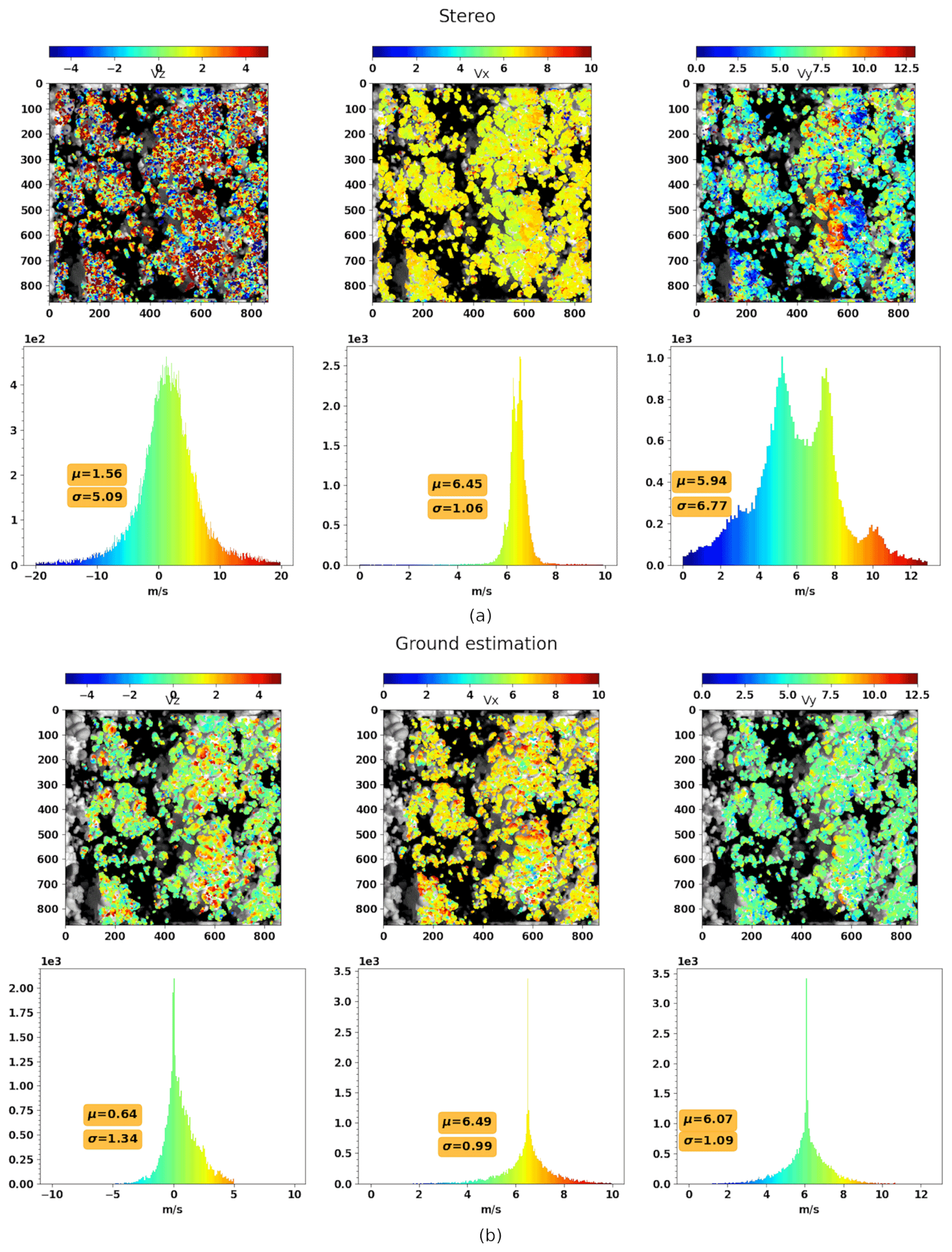
Figure 12(a) STV (stereo velocity) from A5–A6. Top part from left to right: the components z, x, and y of the retrieved velocity STV. Bottom part from left to right: z, x, y distributions. (b) Same as in panel (a) but for GEV (ground estimation velocity).
Similar results (not shown) have been obtained for other pairs of acquisitions, with small differences for the mean values of the velocity and larger dispersion for the ST velocities in comparison to the ground estimate. As discussed previously, the two methods have their own sources of error, with the retrieval relying on image data, whereas the GT velocities are ultimately derived from the physical model. Furthermore, while the retrieval method is based on finding matching points, the GT method relies on measuring cloud-to-cloud distance along the local normal. These two elements certainly contribute to the discrepancy observed. This can be reduced by tracking the position of a group of tie points over several acquisitions, to which we turn next.
5.4 Velocity vectors from ST and GT point clouds via point tracking
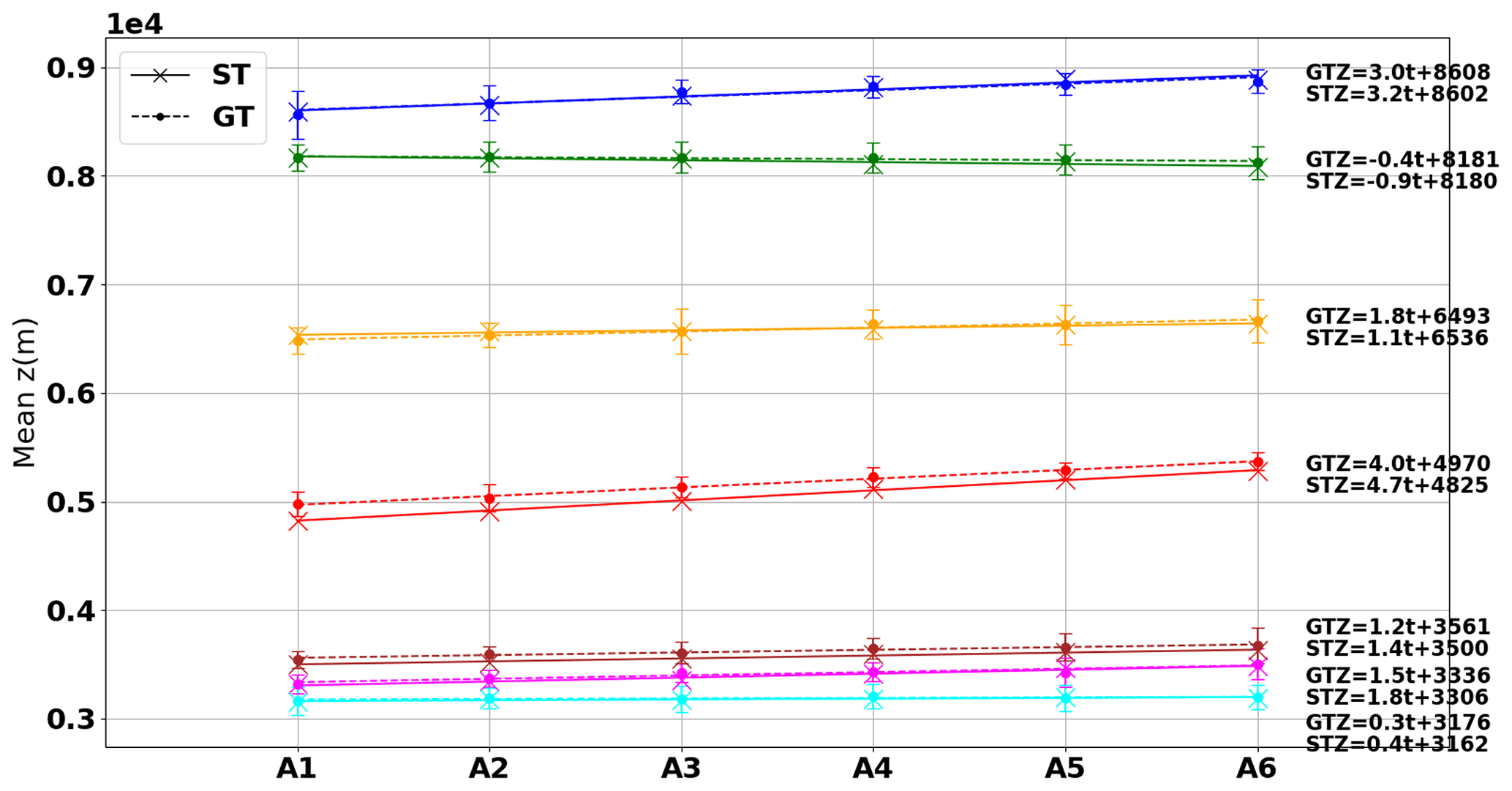
Following the idea mentioned at the end of the previous paragraph, an alternative way for comparing the ST and GT velocities consists in taking the slope of the regression line (over several acquisitions) of the mean X, Y, Z for a given set of tie points. In what follows, seven clusters of tie points from different cloud cells, each identified by a specific colour, as in Fig. 13a, were tracked from A1 (far from nadir) to A6 (close to nadir) by applying MGM every two acquisitions (A1 ⇒ A2, A2 A6). For each cluster of points and for each acquisition, 3D space coordinates are retrieved via image-to-space mapping through 3D reconstruction, as explained in Sect. 4.1. The same sets of points are shown in 3D space (top view, X–Y plane) in Fig. 13b together with the GT point clouds (grey points) for each acquisition. Each group of points, with space coordinates (X, Y, Z), is contained in the rectangular region defined by (Xmin, Xmax) and (Ymin, Ymax), as is shown in the figure inset (light blue rectangle) for the red points of acquisition A6. The same light blue area was divided into 10×10 atmospheric columns (notice red grid), from each of which the uppermost point of the GT point cloud was extracted (black points – GT max). This is justified by the visibility of the GT cloud top. We compare the mean value of Z for the red points (ST points) to the mean value of Z for the black points (GT points). In Fig. 14, the mean ST Z and mean GT Z values are plotted as a function of the acquisition (time) together with the regression lines and SD as error bars. The slope of the regression lines for each cluster gives the mean vertical velocity over the six acquisitions. The agreement between mean ST Z and mean GT Z is good (within the error range) and shows that the cloud development velocity can be estimated with good accuracy over a time interval of 100 s, for instance, as it was done in this case. Lastly, it should be noticed that, with this second approach, we can compensate for the attitude errors of the platforms. However, these sources of error – and likewise, the satellite position error – have not been taken into account to carry out this work that is instead based on realistic but perfect images – “perfect” in that neither radiometric nor attitude errors have been accounted for, as they are out of the scope of this paper.
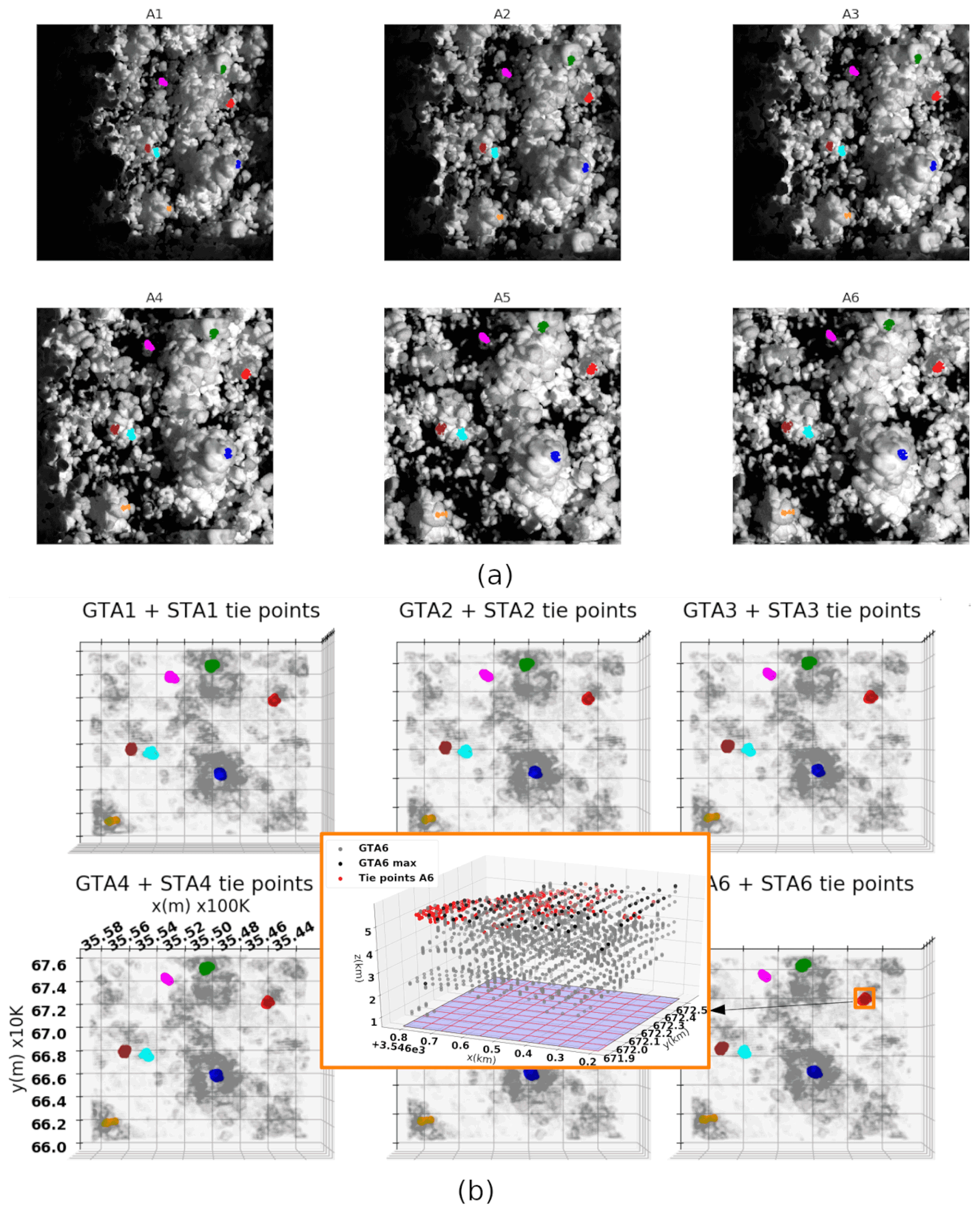
Figure 13(a) Image tie points tracked from simulations A1 to A6 via MGM. Each group of points is associated with a given colour. (b) ST tie points from panel (a) in 3D space and GT point clouds from A1 to A6. Zoomed-in inset showing the atmospheric columns for point selection from the GT point cloud.
A method to retrieve the 3D cloud envelope and 3D cloud development velocity from satellite imagery was presented. As actual data from the CLOUD cameras of the C3IEL mission are not yet available, multi-angular simulated images were used. These were obtained via SAM and the image renderer Mitsuba for a shallow cumulus case and with Meso-NH and the 3D radiative transfer code 3DMCPOL, coupled with an orbit and geometric model simulator, for a deep convective cloud case. Such simulations are realistic in that they were obtained accounting for the geometric camera model, while images are considered “perfect” in that neither radiometric nor geometric noises were taken into account. Cloud geometry retrieval from pairs or triplets of images was attained via 3D stereo reconstruction and was tested against the reference point cloud derived from the physical properties output of the cloud models. The error associated with the cloud geometry retrieval, quantified in terms of RMSE (<40 m) and bias (<30 m), was obtained by measuring cloud-to-cloud distance between retrieved and reference point cloud. The inter-acquisition cloud velocity was instead retrieved by identifying matching cloud features from two consecutive acquisitions (for instance, A1, A2) of the same cloud scene via MGM. The 3D reconstructed point cloud for each acquisition is then used to map the matching cloud features from image to space. The inter-acquisition velocity vector, derived from the retrieved space coordinates (X1, Y1, Z1, X2, Y2, Z2), is the ratio of the space travelled by each tie point to the inter-acquisition time step (20 s). The results were compared against a ground estimate of cloud development velocity that was obtained via a completely independent method that relies on minimising the RMSE of the reference cloud top between two acquisitions and on measuring cloud-to-cloud distance. The mean velocities retrieved from the images and from the ground estimation are in close agreement, although the ST velocities, relying on matching cloud features from two consecutive acquisitions, are more dispersed than the GE velocities derived instead from cloud-to-cloud distance. A more sophisticated assessment for the stereo velocity would require applying the same tracking method used for the images to track the movement of identified cloud structures from the GT point clouds. In the meantime, we developed an easy workaround that consists of tracking a cluster of points over several acquisitions. The slope of the regression line to the mean Z position of a set of matching cloud features, identified over several acquisitions, gives the mean velocity. This method was applied to the point clouds derived from the images and to those derived from the physical model. Results from this second comparison show that an estimate of the stereo velocity can be achieved with good accuracy (within the error range). The cumulus case was not simulated via 3DMCPOL because of time constraints associated with the high computational cost of such calculations. However, in the future, to generalise our results, we plan to test our methods for other cloud types, scenes, and solar geometries. This will be done by taking into account radiometric noise and image distortion as well as satellite orientation and position errors. This will allow for the quantification of the degradation of the results obtained here for “perfect simulations”.
Data are available upon request. The stereo retrieval algorithm s2p used to carry out this work is an open freeware software.
PD and CC conceived the original idea. DaR, RB, YYS, and DiR helped to supervise the project. CC and VH carried out the image simulations. DiR and VH provided the output of the physical cloud models. RB, LF, PD, and VH did the modelling of the geometric camera models. PD performed the computations and tested the retrieval methods. CC and DaR supervised the findings of this work. All authors discussed the results and contributed to the final manuscript. PD wrote the manuscript with support from CC, DiR, RB, and YYS. All authors provided critical feedback and helped to shape the research, analysis, and manuscript.
The contact author has declared that none of the authors has any competing interests.
Publisher’s note: Copernicus Publications remains neutral with regard to jurisdictional claims in published maps and institutional affiliations.
The CNES is acknowledged for the first author contract support. Clément Strauss is acknowledged for the LES modelling of the cumulonimbus cloud while Michael Fisher and Jacob Shpund for their contribution to the Mitsuba and LES simulations of the cumulus case, respectively. François Thieuleux is acknowledged for his contribution to the 3DMCPOL radiative transfer computations and Eric Defer for his critical feedback.
This research has been supported by the Centre National d'Etudes Spatiales (TOSCA/CNES (grant nos. 5414/MTO/4500065502 and 6728/MTO/4500069332)) and the Israel Ministry of Science and Technology (MOST; grant no. 2-17377).
This paper was edited by Bernhard Mayer and reviewed by two anonymous referees.
Adler, R. F. and Fenn, D. D.: Thunderstorm vertical velocities estimated from satellite data, J. Atmos. Sci., 36, 1747–1754, https://doi.org/10.1175/1520-0469(1979)036<1747:TVVEFS>2.0.CO;2, 1979.
Aides, A., Levis, A., Holodovsky, V., Schechner, Y. Y., Althausen, D., and Vainiger, A.: Distributed Sky Imaging Radiometry and Tomography, in: 2020 IEEE International Conference on Computational Photography (ICCP), 24–26 April 2020, St. Louis, MO, USA, 1–12, https://doi.org/10.1109/ICCP48838.2020.9105241, 2020.
Baran, A. J., Francis, P. N., Labonnote, L., and Doutriaux-Boucher, M.: A scattering phase function for ice cloud: Tests of applicability using aircraft and satellite multi-angle multi-wavelength radiance measurements of cirrus, Q. J. Roy. Meteor. Soc., 127, 2395–2416, https://doi.org/10.1002/qj.49712757711, 2001.
Baran, A. J., Cotton, R., Furtado, K., Havemann, S., Labonnote, L., Marenco, F., Smith, A., and Thelen, J.: A self consistent scattering model for cirrus. II: The high and low frequencies, Q. J. Roy. Meteor. Soc., 140, 1039–1057, https://doi.org/10.1002/qj.2193, 2014.
Bony, S., Stevens, B., Frierson, D. , Jakob, C., Kageyama, M., Pincus, R., Shepherd, T. G., Sherwood, S. C., Siebesma, A. P., Sobel, A. H., Watanabe, M., and Webb, M. J.: Clouds, circulation and climate sensitivity, Nat. Geosci., 8, 261–268, https://doi.org/10.1038/ngeo2398, 2015.
Buades, A. and Facciolo, G.: Reliable Multiscale and Multiwindow Stereo Matching, SIAM J. Imaging Sci., 8, 888–915, https://doi.org/10.1137/140984269, 2015.
CloudCompare: CloudCompare, version 2.11.1, GPL software, http://www.cloudcompare.org/ (last access: 10 November 2021), 2010.
Collis, S., Protat, A., May, P., and Williams, C.: Statistics of Storm Updraft Velocities from TWP-ICE Including Verification with Profiling Measurements, J. Appl. Meteorol. Clim., 52, 1909–1922, https://doi.org/10.1175/JAMC-D-12-0230.1, 2013.
Cornet, C., C-Labonnote, L., and Szczap, F.: Three-dimensional polarized Monte Carlo atmospheric radiative transfer model (3DMCPOL): 3D effects on polarized visible reflectances of a cirrus cloud, J. Quant. Spectrosc. Ra., 111, 174–186, https://doi.org/10.1016/j.jqsrt.2009.06.013, 2010.
Cornet, C., C.-Labonnote, L., Waquet, F., Szczap, F., Deaconu, L., Parol, F., Vanbauce, C., Thieuleux, F., and Riédi, J.: Cloud heterogeneity on cloud and aerosol above cloud properties retrieved from simulated total and polarized reflectances, Atmos. Meas. Tech., 11, 3627–3643, https://doi.org/10.5194/amt-11-3627-2018, 2018.
Cuxart, J., Bougeault, P., and Redelsperger, J. L.: A turbulence scheme allowing for mesoscale and large-eddy simulations, Q. J. Roy. Meteor. Soc., 126, 1–30, https://doi.org/10.1002/qj.49712656202, 2000.
de Franchis, C., Meinhardt-Llopis, E., Michel, J., Morel, J.-M., and Facciolo, G.: An automatic and modular stereo pipeline for pushbroom images, ISPRS Ann. Photogramm. Remote Sens. Spatial Inf. Sci., II-3, 49–56, https://doi.org/10.5194/isprsannals-II-3-49-2014, 2014.
Diner, D. J., Xu, F., Garay, M. J., Martonchik, J. V., Rheingans, B. E., Geier, S., Davis, A., Hancock, B. R., Jovanovic, V. M., Bull, M. A., Capraro, K., Chipman, R. A., and McClain, S. C.: The Airborne Multiangle SpectroPolarimetric Imager (AirMSPI): a new tool for aerosol and cloud remote sensing, Atmos. Meas. Tech., 6, 2007–2025, https://doi.org/10.5194/amt-6-2007-2013, 2013.
Donner, L. J., O'Brien, T. A., Rieger, D., Vogel, B., and Cooke, W. F.: Are atmospheric updrafts a key to unlocking climate forcing and sensitivity?, Atmos. Chem. Phys., 16, 12983–12992, https://doi.org/10.5194/acp-16-12983-2016, 2016.
Facciolo, G., de Franchis, C., and Meinhardt, E.: MGM: A Significantly More Global Matching for Stereovision, in: Proceedings of the British Machine Vision Conference (BMVC), edited by: Xie, X., Jones, M. W., and Tam, G. K. L., Swansea, UK, 7–10 September 2015, BMVA Press, 90.1–90.12, https://doi.org/10.5244/C.29.90, 2015.
Freud, E. and Rosenfeld, D.: Linear relation between convective cloud drop number concentration and depth for rain initiation, J. Geophys. Res., 117, D02207, https://doi.org/10.1029/2011JD016457, 2012.
Giangrande, S. E., Collis, S., Straka, J., Protat, A., Williams, C., and Krueger, S.: A Summary of Convective-Core Vertical Velocity Properties Using ARM UHF Wind Profilers in Oklahoma, J. Appl. Meteorol. Clim., 52, 2278–2295, https://doi.org/10.1175/JAMC-D-12-0185.1, 2013.
Girardeau-Montaut, D., Roux, M., Marc, R., and Thibault, G.: Change detection on points cloud data acquired with a ground laser scanner, ISPRS WG III/3, III/4, V/3 Workshop “Laser scanning 2005”, Enschede, the Netherlands, 12–14 September 2005.
Hamada, A. and Takayabu, Y. N.: Convective cloud top vertical velocity estimated from geostationary satellite rapid-scan measurements, Geophys. Res. Lett., 43, 5435–5441, https://doi.org/10.1002/2016GL068962, 2016.
Heymsfield, G. M., Tian, L., Heymsfield, A. J., Li, L., and Guimond, S.: Characteristics of deep tropical and subtropical convection from nadir-viewing high-altitude airborne Doppler radar, J. Atmos. Sci., 67, 285–308, https://doi.org/10.1175/2009JAS3132.1, 2010.
Horvath, A. and Davies, R.: Feasibility and Error Analysis of Cloud Motion Wind Extraction from Near-Simultaneous Multiangle MISR Measurements, J. Atmos. Ocean. Tech., 18, 591–608, https://doi.org/10.1175/1520-0426(2001)018<0591:FAEAOC>2.0.CO;2, 2001a.
Horvath, A. and Davies, R.: Simultaneous retrieval of cloud motion and height from polar-orbiter multiangle measurements, Geophys. Res. Lett., 28, 2915–2918, https://doi.org/10.1029/2001GL012951, 2001b.
Kelly, M. A., Wu, D. L., Boldt, J., Morgan, F., Wilson, J. P., Goldberg, A. C., Yee, J. H., Carr, J. L., Heidinger, A., and Stoffler, R.: A New Approach to Stereo Observations of Clouds, AGU Fall Meeting Abstracts, #A31G-2913, A31G-2913, 2018.
Khairoutdinov, M. F. and Randall, D., A.: Cloud Resolving Modeling of the ARM Summer 1997 IOP: Model Formulation, Results, Uncertainties, and Sensitivities, J. Atmos. Sci., 60, 607–625, https://doi.org/10.1175/1520-0469(2003)060<0607:CRMOTA>2.0.CO;2, 2003.
Lac, C., Chaboureau, J.-P., Masson, V., Pinty, J.-P., Tulet, P., Escobar, J., Leriche, M., Barthe, C., Aouizerats, B., Augros, C., Aumond, P., Auguste, F., Bechtold, P., Berthet, S., Bielli, S., Bosseur, F., Caumont, O., Cohard, J.-M., Colin, J., Couvreux, F., Cuxart, J., Delautier, G., Dauhut, T., Ducrocq, V., Filippi, J.-B., Gazen, D., Geoffroy, O., Gheusi, F., Honnert, R., Lafore, J.-P., Lebeaupin Brossier, C., Libois, Q., Lunet, T., Mari, C., Maric, T., Mascart, P., Mogé, M., Molinié, G., Nuissier, O., Pantillon, F., Peyrillé, P., Pergaud, J., Perraud, E., Pianezze, J., Redelsperger, J.-L., Ricard, D., Richard, E., Riette, S., Rodier, Q., Schoetter, R., Seyfried, L., Stein, J., Suhre, K., Taufour, M., Thouron, O., Turner, S., Verrelle, A., Vié, B., Visentin, F., Vionnet, V., and Wautelet, P.: Overview of the Meso-NH model version 5.4 and its applications, Geosci. Model Dev., 11, 1929–1969, https://doi.org/10.5194/gmd-11-1929-2018, 2018.
Lague, D., Brodu, N., and Leroux, J.: Accurate 3D comparison of complex topography with terrestrial laser scanner: application to the Rangitikei canyon (N-Z), ISPRS J. Photogram., 82, 10–26, https://doi.org/10.1016/j.isprsjprs.2013.04.009, 2013.
LeMone, M. A. and Zipser, E. J.: Cumulonimbus vertical velocity events in GATE. Part I: Diameter, intensity and mass flux, J. Atmos. Sci., 37, 2444–2457, https://doi.org/10.1175/1520-0469(1980)037<2444:CVVEIG>2.0.CO;2, 1980.
Levis, A., Schechner, Y. Y., Aides, A., and Davis, A.: Airborne Three-Dimensional Cloud Tomography, IEEE I. Conf. Comp. Vis. (ICCV), 3379–3387, https://doi.org/10.1109/ICCV.2015.386, 2015.
Loeub, T., Levis, A., Holodovsky, V., and Schechner, Y. Y.: Monotonicity prior for cloud tomography, in: Computer Vision – ECCV 2020. ECCV 2020. Lecture Notes in Computer Science, vol. 12363, edited by: Vedaldi, A., Bischof, H., Brox, T., and Frahm, J. M., Springer-Verlag, 283-299, https://doi.org/10.1007/978-3-030-58523-5_17, 2020.
Lucas, C., Zipser, E., and LeMone, M. A.: Vertical velocity in oceanic convection off tropical Australia, J. Atmos. Sci., 51, 3183–3193, https://doi.org/10.1175/1520-0469(1994)051<3183:VVIOCO>2.0.CO;2, 1994.
Luo, Z. J., Liu, G. Y., andStephens, G. L.: Use of A-Train data to estimate convective buoyancy and entrainment rate, Geophys. Res. Lett., 37, L09804, https://doi.org/10.1029/2010GL042904, 2010.
Luo, Z. J., Jeyaratnam, J., Iwasaki, S., Takahashi, H., and Anderson, R.: Convective vertical velocity and cloud internal vertical structure: An A-Train perspective, Geophys. Res. Lett., 41, 723–729, https://doi.org/10.1002/2013GL058922, 2014.
Martin, G. M., Johnson, D. W., and Spice, A.: The Measurement and Parameterization of Effective Radius of Droplets in Warm Stratocumulus Clouds, J. Atmos. Sci., 51, 1823–1842, https://doi.org/10.1175/1520-0469(1994)051<1823:TMAPOE>2.0.CO;2, 1994.
Masson-Delmotte, V., Zhai, P., Pirani, A., Connors, S.L., Péan, C., Berger, S., Caud, N., Chen, Y., Goldfarb, L., Gomis, M.I., Huang, M., Leitzell, K., Lonnoy, E., Matthews, J. B. R., Maycock, T. K., Waterfield, T., Yelekçi, O., Yu, R., and Zhou, B.: Climate Change 2021: The Physical Science Basis. Contribution of Working Group I to the Sixth Assessment Report of the Intergovernmental Panel on Climate Change (IPCC), Cambridge University Press, Cambridge, United Kingdom and New York, NY, USA, https://doi.org/10.1017/9781009157896, in press, 2022.
Mayer, B.: Radiative transfer in the cloudy atmosphere, EPJ Web Conf., 1, 75–99, https://doi.org/10.1140/epjconf/e2009-00912-1, 2009.
Mitra, A., Di Girolamo, L., Hong, Y., Zhan, Y., and Mueller, K. J.: Assessment and error analysis of Terra-MODIS and MISR cloud-top heights through comparison with ISS-CATS lidar, J. Geophys. Res.-Atmos., 126, e2020JD034281, https://doi.org/10.1029/2020JD034281, 2021.
Pinty, J. P. and Jabouille, P.: A mixed-phase cloud parameterization for use in mesoscale non-hydrostatic model: simulations of a squall line and of orographic precipitations, in: Conf. on Cloud Physics, Everett, WA, 17–21 August 1998, American Meteorological Society [preprint], 217–220, 1998.
Ronen, R., Schechner, Y. Y., and Eytan, E.: 4D Cloud Scattering Tomography, in: Proceedings of the IEEE/CVF International Conference on Computer Vision (ICCV), Montreal, QC, Canada, 10–17 October 2021, 5500–5509, https://doi.org/10.1109/ICCV48922.2021.00547, 2021.
Schumacher, C., Stevenson, S., and Williams, C.: Vertical motions of the tropical convective cloud spectrum over Darwin, Australia, Q. J. Roy. Meteor. Soc., 141, 2277–2288, https://doi.org/10.1002/qj.2520, 2015.
Sde-Chen, Y., Schechner, Y. Y., Holodovsky, V., and Eytan, E.: 3DeepCT: Learning volumetric scattering tomography of clouds, in: Proceedings of the IEEE/CVF International Conference on Computer Vision (ICCV), Montreal, QC, Canada, 10–17 October 2021, 5671–5682, https://doi.org/10.1109/ICCV48922.2021.00562, 2021.
Seiz, G. and Davies, R.: Reconstruction of cloud geometry from multi-view satellite images, Remote Sens. Environ., 100, 143–149, https://doi.org/10.1016/j.rse.2005.09.016, 2006.
Seiz, G., Tjemkes, S., and Watts, P.: Multiview Cloud-Top Height and Wind Retrieval with Photogrammetric Methods: Application to Meteosat-8 HRV Observations, J. Appl. Meteorol. Clim., 46, 1182–1195, https://doi.org/10.1175/JAM2532.1, 2007.
Sherwood, S. C., Bony, S., and Dufresne, J.-L.: Spread in model climate sensitivity traced to atmospheric convective mixing, Nature, 505, 37–42, https://doi.org/10.1038/nature12829, 2014.
Strauss, C., Ricard, D., Lac, C., and Verrelle, A.: Evaluation of turbulence parameterizations in convective clouds and their environment based on a large‐eddy simulation, Q. J. Roy. Meteor. Soc., 145, 3195–3217, https://doi.org/10.1002/qj.3614, 2019.
Tao, C. and Hu, Y.: A Comprehensive Study of the Rational Function Model for Photogrammetric Processing, Photogramm. Eng. Rem. S., 67, 1347–1357, 2001.
Takahashi, H., Luo, Z. J., and Stephens, G. L.: Level of neutral buoyancy, deep convective outflow, and convective core: New perspectives based on 5 years of CloudSat data, J. Geophys. Res.-Atmos., 122, 2958–2969, https://doi.org/10.1002/2016JD025969, 2017.
Veikherman D., Aides A., Schechner Y. Y., and Levis, A.: Clouds in the Cloud, in: Computer Vision – ACCV 2014. ACCV 2014. Lecture Notes in Computer Science, vol. 9006, edited by: Cremers, D., Reid, I., Saito, H., and Yang, M. H., Springer, Cham, https://doi.org/10.1007/978-3-319-16817-3_43, 2015.
Weisman, M. L. and Klemp, J. B.: The Structure and Classification of Numerically Simulated Convective Stormsin Directionally Varying Wind Shears, Mon. Weather Rev., 112, 2479–2498, https://doi.org/10.1175/1520-0493(1984)112<2479:TSACON>2.0.CO;2, 1984.
Wenzel, J.: Mitsuba 3, Mitsuba renderer [code], http://www.mitsuba-renderer.org (last access: 11 March 2019), 2010.
Zhang, K., Snavely, N., and Sun, J.: Leveraging vision reconstruction pipelines for satellite imagery, in: Proceedings of the IEEE/CVF International Conference on Computer Vision (ICCV) Workshops, Seoul, Korea, 27–28 October 2019, 2139–2148, https://doi.org/10.1109/ICCVW.2019.00269, 2019.
- Abstract
- Introduction
- Principle of measurement and methodology
- Data: the CLOUD simulations
- 3D cloud envelope: geometry retrieval
- Inter-acquisition cloud development velocity from feature matching and 3D stereo (ST) retrieval
- Conclusions
- Code and data availability
- Author contributions
- Competing interests
- Disclaimer
- Acknowledgements
- Financial support
- Review statement
- References