the Creative Commons Attribution 4.0 License.
the Creative Commons Attribution 4.0 License.
 | 17 Nov 2022
Evaluation of the methane full-physics retrieval applied to TROPOMI ocean sun glint measurements
Tobias Borsdorff
Mari C. Martinez-Velarte
Andre Butz
Otto P. Hasekamp
Lianghai Wu
Jochen Landgraf
The TROPOspheric Monitoring Instrument (TROPOMI), due to its wide swath, performs observations over the ocean in every orbit, enhancing the monitoring capabilities of methane from space. In the short-wave–infrared (SWIR) spectral band ocean surfaces are dark except for the specific sun glint geometry, for which the specular reflectance detected by the satellite provides a signal that is high enough to retrieve methane with high accuracy and precision. In this study, we build upon the RemoTeC full-physics retrieval algorithm for land measurements, and we retrieve 4 years of methane concentrations over the ocean from TROPOMI. We fully assess the quality of the dataset by performing a validation using ground-based measurements of the Total Carbon Column Observing Network (TCCON) from near-ocean sites. The validation results in an agreement of % ( ppb) for the mean bias and station-to-station variability, which show that glint measurements comply with the mission requirement of precision and accuracy below 1 %. Comparison to ocean measurements from the Greenhouse gases Observing SATellite (GOSAT) results in a bias of % ( ppb), equivalent to the comparison of measurements over land. The full-physics algorithm simultaneously retrieves the amount of atmospheric methane and the physical scattering properties of the atmosphere from measurements in the near-infrared (NIR) and SWIR spectral bands. Based on the scattering properties of the atmosphere and ocean surface reflection we further validate retrievals over the ocean. Using the “upper-edge” method, we identify a set of ocean glint observations where scattering by aerosols and clouds can be ignored in the measurement simulation to investigate other possible error sources such as instrumental errors, radiometric inaccuracies or uncertainties related to spectroscopic absorption cross-sections. With this ensemble we evaluate the RemoTeC forward model via the validation of the total atmospheric oxygen (O2) column retrieved from the O2 A-band, as well as the consistency of XCH4 retrievals using sub-bands from the SWIR band, which show a consistency within 1 %. We discard any instrumental and radiometric errors by a calibration of the O2 absorption line strengths as suggested in the literature.
- Article
(6473 KB) - Full-text XML
- BibTeX
- EndNote


Methane measurements over the ocean from the TROPOspheric Monitoring Instrument (TROPOMI) provide unprecedented monitoring capabilities for this potent greenhouse gas. Ocean measurements from satellite instruments in the short-wave–infrared spectral band are challenging due to low levels of reflected sunlight from water surfaces that may result in a low signal-to-noise ratio. For observations made under the specific sun glint geometry that provides specular reflection, the reflectance is strong compared to the off-glint dark ocean scenes. It provides a signal that is high enough to retrieve methane concentrations that comply with the mission's strict precision and accuracy requirements for atmospheric inversion analysis to estimate methane sources and sinks.
TROPOMI is a nadir-viewing spectrometer that measures sunlight scattered back by Earth's surface and atmosphere. It uses a push broom scanning technique, and with its 2600 km wide swath, it obtains global coverage every day. The measurement approach allows TROPOMI to perform observations under sun glint geometry in every orbit. This is different from other instruments that use a pointing mechanism to observe scenes under sun glint geometries, resulting in a reduced coverage compared to that of TROPOMI. The instrument on board the Greenhouse gases Observing SATellite (GOSAT) performs point measurements with a spatial resolution of about 10 km, and the Orbiting Carbon Observatory-2 (OCO-2) obtains eight cross-track footprints, resulting in a narrow swath of approximately 10 km. The sun glint area (defined geometrically by the sun glint angle in Eq. A1) depends on the solar azimuth and zenith angles, resulting in a seasonal cycle on the global ocean coverage such that different latitudinal bands are covered throughout the year (Fig. A1).
In order to retrieve methane from ocean sun glint TROPOMI observations, we build upon the full-physics retrieval algorithm applied to measurements over land that simultaneously retrieves the amount of methane in the atmosphere and the scattering properties of aerosol and cirrus using both the near-infrared (NIR; 757–774 nm) and short-wave–infrared (SWIR; 2305–2385 nm) spectral bands. The full-physics retrieval uses the modification by aerosols of the strong absorption lines, the oxygen (O2) A-band in the NIR and methane (CH4) and water (H2O) in the SWIR, to obtain information about scattering in the atmosphere. The RemoTeC algorithm has already been successfully applied to retrieve methane and carbon dioxide from sun glint ocean observations from GOSAT (e.g. Wu et al., 2020) and OCO-2 (e.g. Wu et al., 2018). Sources of systematic errors in the full-physics retrievals of greenhouse gases include among other things instrumental errors and noise, spectroscopic uncertainties, and inaccuracies in the characterization of scattering processes by aerosols and clouds in the forward model. Even though the full-physics retrieval accounts explicitly for atmospheric scattering effects, these pose the biggest challenge for greenhouse gas retrievals. It is therefore the error source that has been analysed most extensively in the literature (e.g. Butz et al., 2010; Houweling et al., 2005). To account for it, usually empirical posterior bias corrections are applied to the retrieved methane and carbon dioxide abundances.
For ocean observations, most of the light detected by the satellite in the sun glint geometry comes from the direct reflection of solar light with very little contribution from diffuse scattering, whereas over land single and multiple scattering contribute substantially to the top-of-atmosphere reflectance. Therefore errors due to unaccounted light path modifications by scattering processes for retrievals over ocean can be substantially different from those over land. The magnitude and sign of these errors depend on the surface reflection, which is key to determining the effective optical path through the atmosphere (Aben et al., 2007). Over land, both light path enhancement and shortening can happen. For scenes with moderate to high surface reflectance, atmospheric scattering results in an enhancement of the light path due to multiple scattering, leading to an overestimation of the trace gas if scattering is not properly accounted for. For scenes with low surface reflectance, atmospheric scattering results mainly in a shortening of the light path as light might be scattered back before reaching the surface or absorbed at the surface. Because a relatively strong scattering event is needed at the surface for light path enhancement, retrievals over the ocean mostly suffer from underestimation if scattering processes are not taken into account (Butz et al., 2013).
Based on the rationale explained above, Butz et al. (2011) proposed the so-called “upper-edge” method to identify an ensemble of ocean scenes with negligible scattering effects from which it is possible to discriminate between errors related to scattering processes and other sources like instrumental errors or spectroscopic uncertainties (Butz et al., 2013). The method assumes that when applying a retrieval based on an atmosphere with only molecular Rayleigh scattering, the retrieved oxygen (or surface pressure) is underestimated for most of the scenes, bounded by an upper edge that corresponds to scenes where aerosol scattering can be ignored. This method has been applied to several retrieval algorithms for GOSAT measurements (e.g. Butz et al., 2011; Crisp et al., 2012; Yoshida et al., 2013; Cogan et al., 2012). These studies found a bias in the retrieved O2 and surface pressure for the upper-edge ensemble, and even though the cause of the bias remained unclear (e.g. Yoshida et al., 2013), they all estimated a scaling factor of the O2 column density of similar magnitude. This scaling factor was applied to the O2 absorption line strengths, but because of the limited spatial coverage of the GOSAT data, the assessment of the scaling factor effect on the retrieved greenhouse gas concentrations was limited in all these studies.
In this study we apply an optimized regularization scheme to the RemoTeC full-physics retrieval algorithm to obtain 4 years of methane concentrations over the ocean from TROPOMI sun glint observations (Sect. 3), and we perform a full assessment of the quality of the dataset. First, the same way as for measurements over land, we validate sun glint ocean measurements using ground-based measurements of the Total Carbon Column Observing Network (TCCON) from near-ocean sites (Sect. 4.1). We also compare methane from TROPOMI with retrievals from GOSAT (Sect. 4.2), and we evaluate the performance of the cloud and aerosol filter by analysing individual scenes for which dust outbreaks pose a challenge to the full-physics retrieval (Sect. 4.3). Due to the considerable amount of TROPOMI data over the ocean, we can further evaluate the retrievals over the ocean by applying the upper-edge method (Sect. 5). The purpose of applying the method is twofold: on the one hand, to diagnose the forward model for the O2 A-band and validate the retrieved O2 and on the other hand to obtain an ensemble of scenes free of scattering effects to investigate other possible sources of error in the forward model.
We retrieve methane from TROPOMI with the RemoTeC full-physics algorithm, described in detail by Hu et al. (2016) and Lorente et al. (2021), as well as in the Algorithm Theoretical Basis Document (Hasekamp et al., 2021). The full-physics approach simultaneously retrieves the amount of atmospheric methane (CH4) and the physical scattering properties of the atmosphere from measurements (y) of sunlight scattered back by the Earth's surface and the atmosphere in the near-infrared (NIR; 757–774 nm) and short-wave–infrared (SWIR; 2305–2385 nm) spectral bands.
The forward model (F) employs the LINTRAN V2.0 radiative transfer model in its scalar approximation to simulate atmospheric light scattering and absorption in a plane-parallel atmosphere (Schepers et al., 2014; Landgraf et al., 2001). In the forward model, surface reflection is modelled differently for land and ocean. For land scenes, surface is assumed to be Lambertian, which means that light is reflected isotropically without accounting for the geometry-dependent properties of the surface reflection. For ocean scenes, surface reflection is modelled using the wind-speed-dependent Cox–Munk reflection model (Cox and Munk, 1954) together with a wavelength-dependent Lambertian term. Wind speed and surface pressure information are obtained from the ECMWF operational analysis product and are therefore not retrieved.
The retrieval algorithm aims to find the state vector x that contains CH4 partial sub-column number densities by solving the minimization problem:
where describes the Euclidian norm, y is the vector containing the spectral measurements, Sy is the diagonal measurement error covariance matrix that contains the noise estimate, F(x) is the forward model applied to the state vector x, γ is the regularization parameter, W is a diagonal unity weighting matrix that ensures that only the target absorber CH4 and the scattering parameters contribute to its norm (Hu et al., 2016), and xa is the a priori state vector. The retrieval state vector contains CH4 partial sub-column number densities at 12 equidistant pressure layers. The total columns of the interfering absorbers CO and H2O are also retrieved, together with the effective aerosol total column, size and height parameter of the aerosol power law distribution as well as spectral shift and fluorescence in the NIR band. A Lambertian surface albedo in both the NIR and SWIR spectral range and its first-order spectral dependence is also retrieved. Because of the different treatment of surface reflection in the forward model for land and ocean scenes, the physical description of the surface albedo is different, and for ocean scenes it can lead to negative retrieved values. The final product of the retrieval is the methane total column-averaged dry-air mole fraction (XCH4), calculated from the methane vertical sub-column elements xi and the dry-air column Vair,dry calculated with meteorology input from ECMWF.
In Lorente et al. (2021), we optimized the regularization parameter γ for the target absorber CH4 and for each of the scattering parameters separately (effective aerosol distribution height and size parameter and effective aerosol column). This resulted in a more stable performance of the inversion compared to the L-curve method, in which the regularization strength changed at each iteration for every scene (Hu et al., 2016).
To infer XCH4, ocean scenes are too dark, except for the ones under the sun glint geometry where the satellite observes the specular solar reflection at the ocean surface. In this geometry, direct reflection of sunlight from the surface dominates over the diffuse contribution of single and multiple scattering from aerosols. This makes the retrieval over ocean scenes less sensitive to aerosols than over land. Applying RemoTeC to ocean sun glint measurements with its configuration for land retrievals results in an unstable inversion for which particularly the retrieved aerosol height is dominated by noise. As the three effective aerosol parameters in the state vector are regularized separately with a constant regularization parameter for all the scenes (Lorente et al., 2021), we increase the regularization of the effective aerosol height distribution. Consequently, there is on average a 15 % higher convergence rate over ocean than the previous choice of regularization parameters. Applying the same regularization over land has little effect (average global change in XCH4 of ppb for 1 year of data). Therefore, we apply a consistent regularization for both land and ocean retrievals.
Posterior correction
Retrievals over land show an underestimation of XCH4 for scenes with low surface albedo in the short-wave–infrared spectral band. For these scenes, a posterior correction is applied based on the “small area approximation” (O'Dell et al., 2018), which assumes a uniform XCH4 distribution as a function of albedo in several regions around the globe. For each region, a XCH4 reference value is estimated for a surface albedo around 0.2, and then the albedo dependency is obtained for all the regions combined (Lorente et al., 2021). The specific surface albedo value is selected because XCH4 retrieval errors are lower in the SWIR for that albedo range (Guerlet et al., 2013; Aben et al., 2007). The correction is derived using only TROPOMI XCH4, making the correction completely independent of any reference data. The validation with TCCON and GOSAT for land retrievals showed that the posterior correction reduces the regional bias by 6 ppb (Lorente et al., 2021).
For ocean and land scenes the forward model of RemoTeC is inherently different because the description of surface reflection is different (see Sect. 2), so land–ocean contrast in the retrieved XCH4 is not unusual, and there might be reasons to apply a different posterior bias correction for land and ocean observations. Retrievals over ocean do not show any correlation with signal or other retrieved parameters. So based on the global distribution of retrieved XCH4 over ocean and over land we calculate a global correction factor. Even though most of the methane sources are located over land, a correction based on the annual median distribution of methane should not be affected by local emission events. To estimate the correction factor, we calculate the ratio between the median XCH4 over land and over ocean. We compute the median separately for the Northern Hemisphere and Southern Hemisphere to account for the inter-hemispheric XCH4 gradient. Here we limit the analysis to latitudes 60∘ N and 60∘ S as there are no sun glint measurements at larger latitudes (see Appendix A, Fig. A1). For the Northern Hemisphere the ratio of land and ocean median XCH4 is 1.005, and for the Southern Hemisphere it is 1.003. We apply globally the average of the two, resulting in a factor of 1.004.
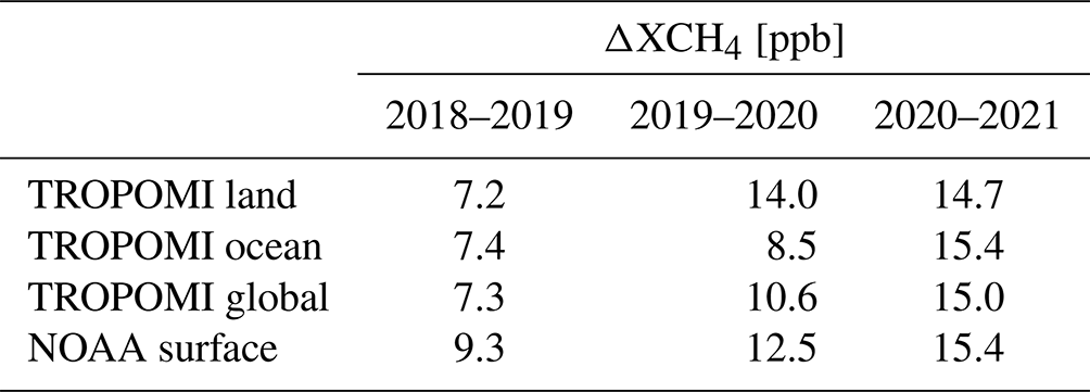
We present 4 years of XCH4 retrieved from TROPOMI measurements based on the retrieval approach explained in Sect. 2, including ocean measurements under sun glint geometry. Figure 1 illustrates the global, yearly average TROPOMI XCH4 both over land and over ocean. Year-to-year distribution reflects the increase in atmospheric XCH4, depicted as well in the time series in Fig. 2, which shows annually averaged TROPOMI XCH4 and surface dry-air mole fraction of CH4 from the marine surface network of the National Oceanic and Atmospheric Administration (NOAA) Earth System Research Laboratory. The TROPOMI global mean XCH4 shows an annual increase with respect to the previous year of 7.3, 10.6 and 15 ppb in 2019, 2020 and 2021, respectively. This increasing trend in the growth rate is also captured by measurements from marine surface sites, assuming full mixing in the atmosphere such that the trends in surface measurements and in the column measured by TROPOMI are comparable. Further breakdown of TROPOMI global average reflects the consistency between ocean sun glint measurements and those over land, with a similar growth rate calculated with each of the measurements separately for 2018–2019 and 2020–2021 (see Table 1). For 2019–2020 a different growth rate is estimated using land (14.0 ppb) and ocean (8.5 ppb) measurements separately. This discrepancy may be due to a difference in coverage over ocean in 2020 and 2019 as a result of a bias in the cloud fraction used for filtering. The VIIRS cloud mask (VCM) used in the S5P-NPP processor of VIIRS data was biased towards higher cloud fractions in the centre of the glint area over the ocean, resulting in a reduced coverage in 2018 and 2019 (see Fig. 1). In March 2020 there was a switch in the cloud mask in favour of the Enterprise cloud mask (ECM), which no longer resulted in a bias in the cloud fraction. Once the VIIRS data are reprocessed with the ECM cloud mask for 2018 and 2019 (foreseen for fall 2022), the cloud fraction used to filter scenes and the coverage over the ocean will be uniform throughout the years.
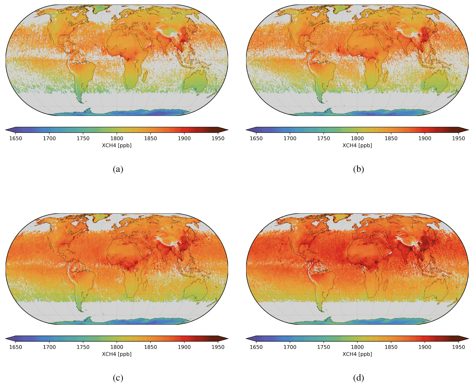
Figure 1Global TROPOMI XCH4 distribution for (a) 2018, (b) 2019, (c) 2020 and (d) 2021, averaged in a cylindrical equal-area grid with a grid at the Equator. TROPOMI XCH4 with the bias correction applied is shown (see Sect. 2.1). The difference in ocean coverage for 2018 and 2019 with respect to 2020 and 2021 is due to a bias in the VIIRS cloud fraction (see Sect. 3).
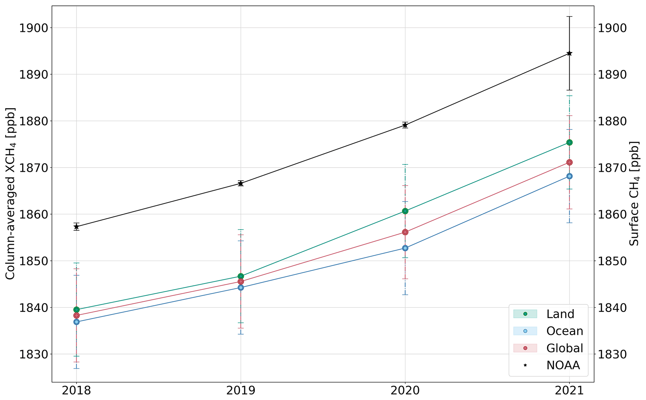
Figure 2Time series of annual mean XCH4 distribution calculated from TROPOMI measurements over land, over ocean and globally (land and ocean) and globally averaged surface CH4 determined from NOAA marine surface sites.
Table 1Atmospheric XCH4 growth rate calculated as the difference between annual mean column-averaged methane measured by TROPOMI over land, over ocean and globally (land and ocean) and surface methane measured by NOAA marine ground-based sites.
The spatial distribution along various coastlines like eastern South Africa and south-eastern Australia shown in Fig. 1 depicts a slight gradient of XCH4 between land and ocean close to the coast. Further analysis of these gradients show that they are partly attributable to the computation of the yearly average that involves different seasonal coverage over land and ocean, as high latitudes over the ocean are only covered partially throughout the year. On the other hand, as mentioned in Sect. 2.1, differences in the forward model between land and ocean may lead to residual differences in the retrieved XCH4. This divergence is reduced by the posterior correction applied to XCH4 retrieved over the ocean based on land retrievals (Sect. 2.1). Particularly over the eastern South African and south-eastern Australian coast the gradients are reduced from 1.0 %–1.5 % to around 0.5 %. The fact that land–ocean gradients are smaller than 1 % reflects the good agreement between land and ocean retrievals and the fitness for purpose of the correction. Note that the estimation of the posterior correction factor is not affected by this spatial and temporal mismatch of the coverage since it involves averages based on multiple latitude ranges.
XCH4 enhancements
TROPOMI XCH4 observations over the ocean further contribute to the monitoring of CH4 emissions thanks to the detection of strong XCH4 enhancements. As an example, Fig. 3 shows single-pass TROPOMI XCH4 measurements over eastern Turkmenistan and the Caspian Sea, where multiple pixels with high XCH4 enhancements are clearly visible. Close to the south coast TROPOMI detected two distinct plumes that originated in oil and gas facilities located inland, from which satellite-based emissions have already been reported (e.g. Varon et al., 2019). On this specific day, the biggest enhancements are found in the Turkmenbashi Bay near multiple point sources (Irakulis-Loitxate et al., 2022) and over the ocean in front of the Cheleken Peninsula, close to locations where VIIRS detected flaring. While for the southernmost emissions relatively strong winds transport the plume northward, in the northernmost area the low wind results in accumulation of air masses; therefore emitted CH4 does not travel further, resulting in XCH4 enhancements as high as 120 ppb over a background of 1870 ppb.
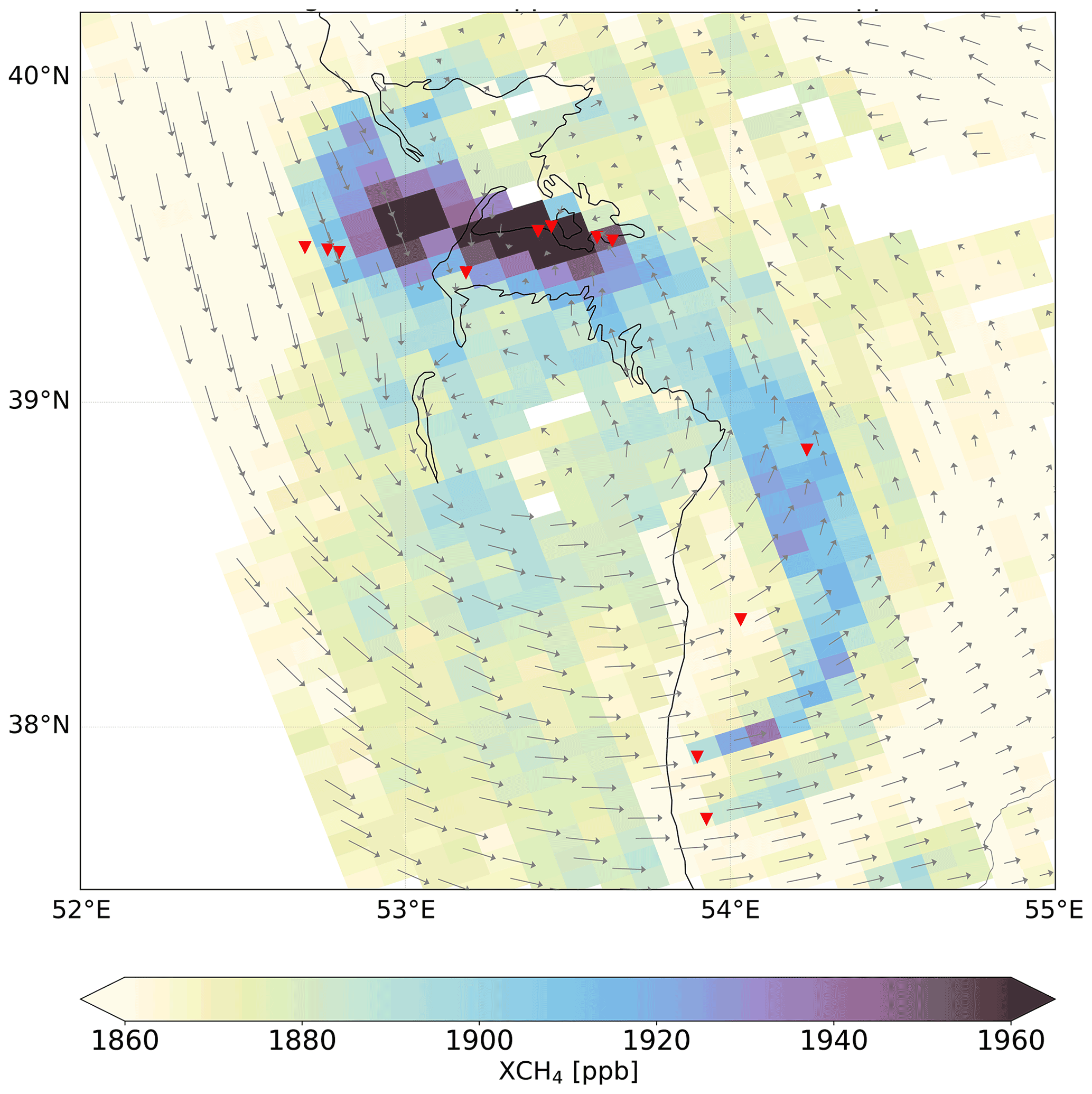
Figure 3TROPOMI XCH4 observations over Turkmenistan and the Caspian Sea on 24 June 2018. Inland oil and gas facilities and over-sea locations where flaring was detected by VIIRS on this specific day are indicated with red triangles. Wind arrows represent ECMWF 10 m wind fields.
The emission quantification methods typically applied to TROPOMI XCH4 data (given their temporal and spatial resolution), like the cross-sectional flux method and the integrated mass enhancement, linearly depend on the detected XCH4 enhancement with respect to the background value. For the particular example shown in Fig. 3, accounting for land pixels only results in a total enhancement (i.e. sum of all per-pixel enhancements) of 663 ppb, while ocean pixels make up to 1816 ppb of XCH4 enhancement. Even if the detected enhancements over the ocean came from offshore emissions or transport from inland, the XCH4 distribution and enhancement are homogeneous and not affected by land–ocean biases in the retrieval. This example highlights the importance of having observations over oceans to accurately quantify the total amount of CH4 emissions.
4.1 Validation with ground-based measurements
In this section, we validate the TROPOMI XCH4 updated dataset (Sect. 3) with ground-based measurements from the Total Carbon Column Observing Network (TCCON) (Wunch et al., 2011) (data version GGG2014, downloaded on 15 December 2021) for TROPOMI measurements over ocean for sun glint geometries. We include the validation for measurements both over ocean and over land to put the results into perspective.
We use TROPOMI XCH4 with a spatial collocation radius of 300 km around each station and a temporal overlap of 2 h for the ground-based measurement and the satellite overpass. We average TROPOMI XCH4 and compare it to the TCCON XCH4, and for all individual paired collocations we estimate the mean bias of TROPOMI–TCCON XCH4 differences and its standard deviation. We then compute the average of the biases of all stations and its standard deviation as a measure of the station-to-station variability as a diagnostic parameter for the regional bias, following the approach in Lorente et al. (2021).
4.1.1 Ocean
In order to validate TROPOMI XCH4 retrievals over ocean, we select stations on islands or inland located close to the coastline (see Table B1) similarly to the validation of measurements from GOSAT and OCO-2 (e.g. Zhou et al., 2016). Figure 4 shows the time series of XCH4 measured by TROPOMI and TCCON for each of the stations for the period November 2017–October 2021. TROPOMI XCH4 sun glint ocean measurements capture the seasonal variability and the year-to-year increase as also captured by TCCON XCH4 measurements. This is true even for stations located close to the tropics (e.g. Burgos), where cloudiness challenges the coverage of TROPOMI XCH4 measurements due to the strict cloud filtering. TROPOMI XCH4 measurements show gaps due to the seasonality of the sun glint geometry throughout the year. Overall, TROPOMI XCH4 sun glint measurements over ocean are biased low by −0.5 % (−8.4 ppb), and the station-to-station variability is 0.3 % (6.3 ppb). The effect of the posterior correction (Sect. 2.1) is to reduce the overall bias from −0.8 % to −0.5 % without any effect on the station-to-station variability as it is a constant correction factor.
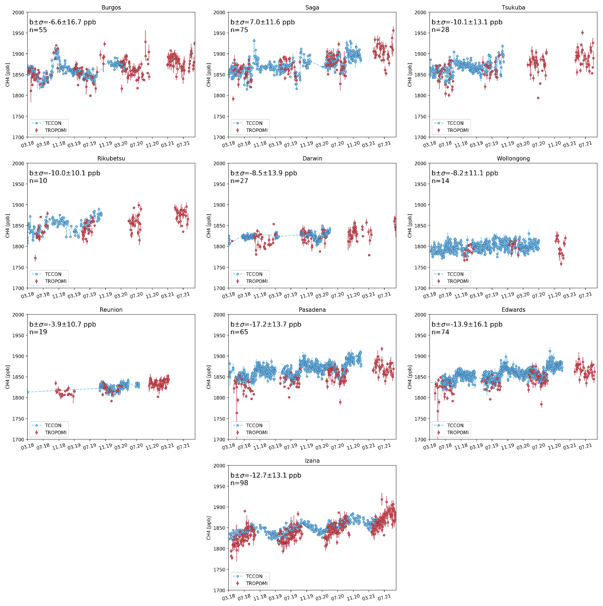
Figure 4Time series of daily averaged XCH4 measurements from TCCON (blue) and TROPOMI over ocean for sun glint geometry (red) collocated with the selected stations for the period 1 March 2018–1 October 2021. TROPOMI measurements over ocean for sun glint geometries around a circle of 300 km radius around each station have been selected for the validation.
Izaña, located on the Canary Islands in Spain, is one of the stations that provides more recent data (see Fig. 4). This station is challenging due to dust outbreaks from the Sahara and also because of the high altitude at which the TCCON instrument is located (2370 m a.s.l.). For this high-altitude station, TROPOMI measurements over ocean and those of the ground-based station look at significantly different atmospheric columns. Therefore, it is necessary to apply an altitude correction to avoid biases due to large height differences (e.g. Sha et al., 2021). As Izaña measurements are always located at a higher altitude than the satellite measurements over ocean, the correction cuts off the partial column below the station height using the prior profile. The validation results are summarized in Table 2.
Table 2Overview of the validation results of TROPOMI XCH4 ocean sun glint measurements with measurements from the TCCON network at selected stations. The table shows the number of collocations, mean bias and standard deviation for each station and the mean bias for all stations and the station-to-station variability. Results are shown for TROPOMI XCH4 with and without the posterior correction applied.
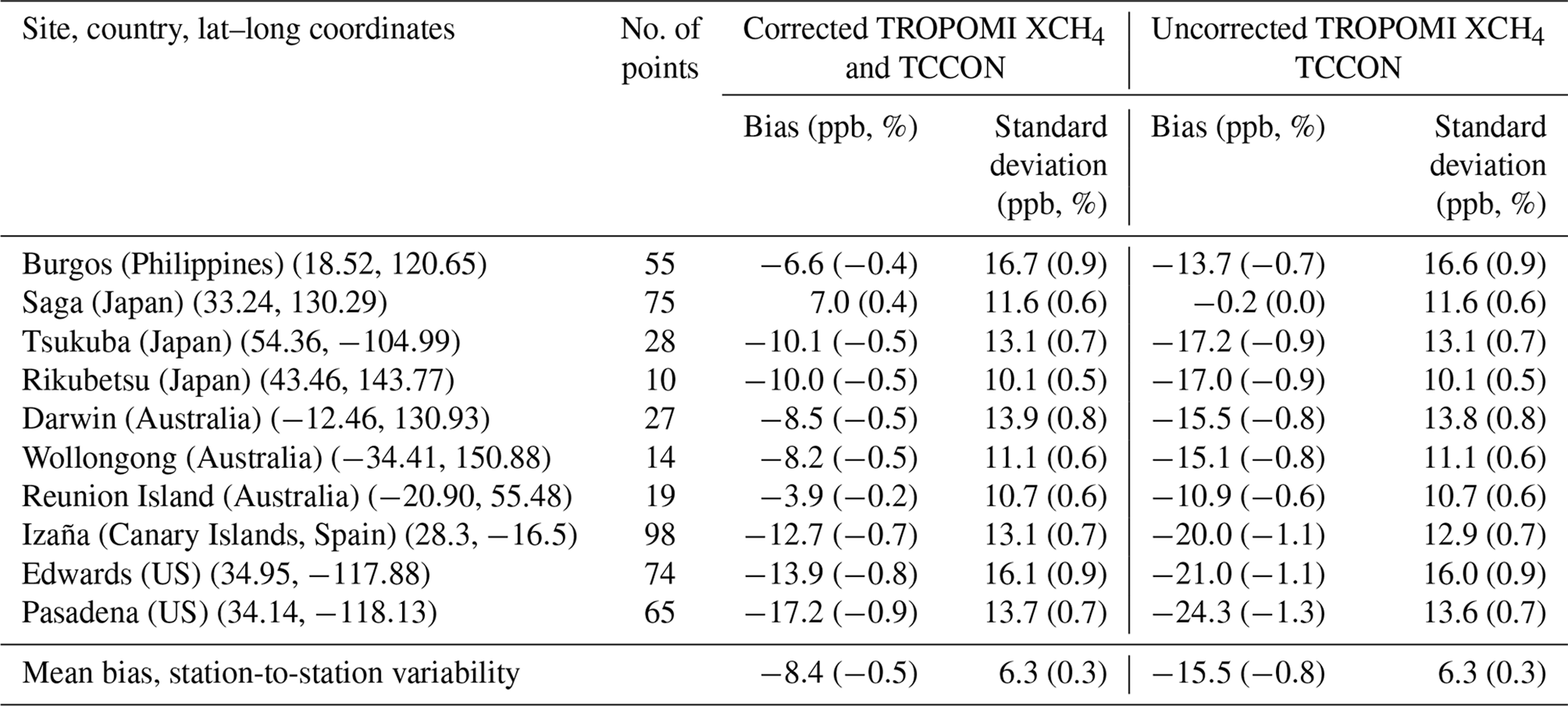
Table 3Overview of the validation results of TROPOMI XCH4 land measurements with measurements from the TCCON network at selected stations. The table shows the number of collocations, mean bias and standard deviation for each station and the mean bias for all stations and the station-to-station variability. Results are shown for TROPOMI XCH4 with and without the albedo bias correction applied.
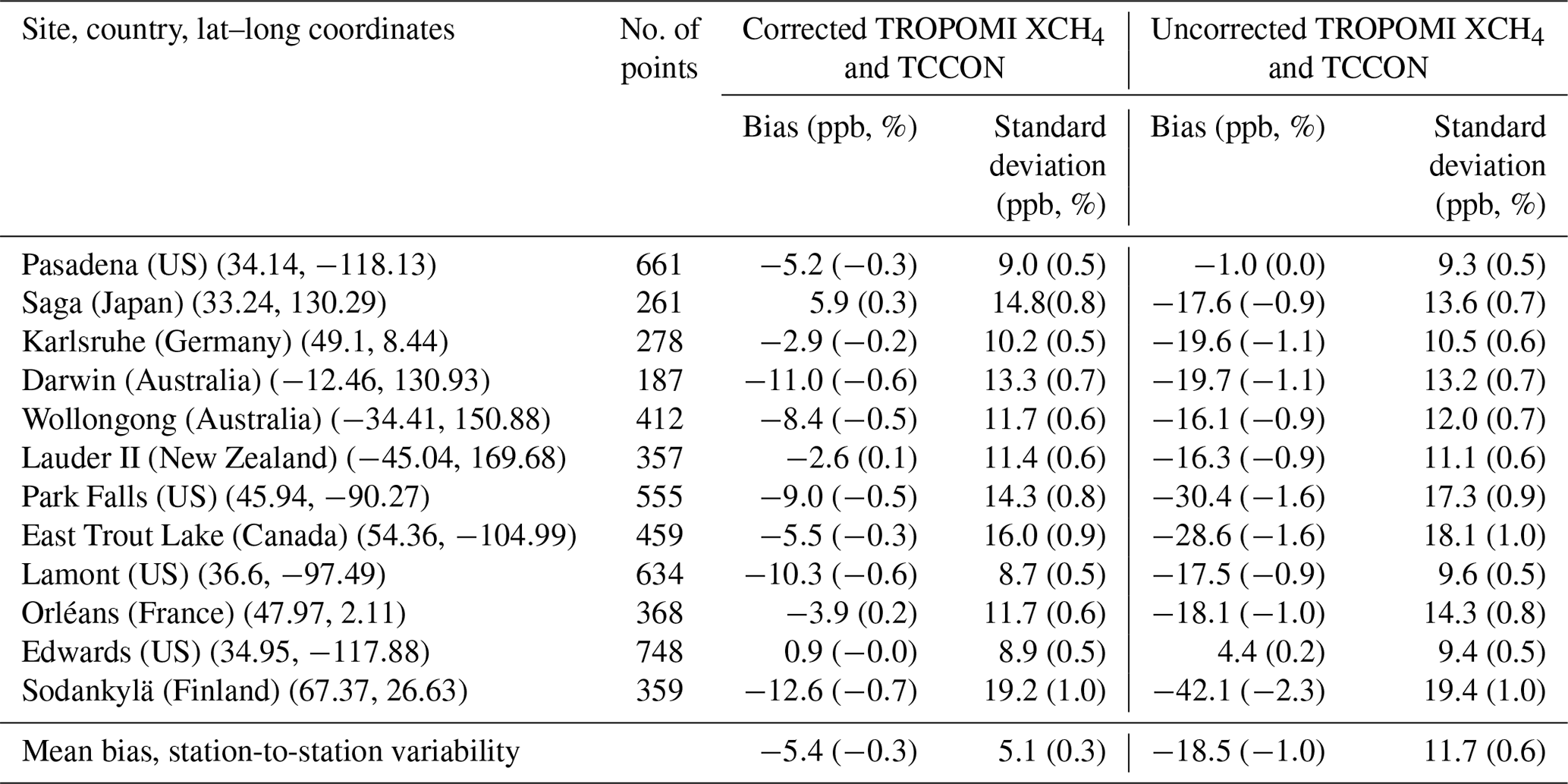
4.1.2 Land
For the validation of measurements over land, we select the same 13 stations (Table B2) as in Lorente et al. (2021) for the results to be comparable between the different versions of the TROPOMI XCH4 dataset. TROPOMI XCH4 over land shows a good agreement with TCCON measurements, with an overall bias and station-to-station variability of −0.3 %. Even before the correction, the overall bias is within 1 %. The posterior correction over land, which depends on the retrieved surface albedo, decreases the overall bias from −1.0 % to −0.3 % and the station-to-station variability from −0.6 % to −0.3 %, stressing the fitness for the purpose of the correction. Based on the magnitude of the overall bias and station-to-station variability for land and ocean retrievals, we can conclude that the data over land and ocean along the coast show a similar data quality. The validation results are summarized in Table 3.
4.2 Comparison with GOSAT
In this section we compare TROPOMI XCH4 with XCH4 retrieved from measurements by the Thermal And Near infrared Sensor for carbon Observations – Fourier Transform Spectrometer (TANSO‐FTS) on board GOSAT. The GOSAT XCH4 product is retrieved using the RemoTeC proxy retrieval, produced at the SRON Netherlands Institute for Space Research in the context of the ESA GreenHouse Gas Climate Change Initiative (GHG CCI) project (Buchwitz et al., 2019, 2017).
We compare XCH4 for the period 1 March 2018–31 December 2020, and we compute the average of daily biases and its standard deviation between TROPOMI and GOSAT measurements gridded in a grid. Figure 5 shows XCH4 retrieved from GOSAT (Fig. 5a) and TROPOMI (Fig. 5b). While over land the coverage of both satellites is relatively comparable after performing the long-term temporal average and spatial gridding, over the ocean TROPOMI is able to cover a greater area than GOSAT thanks to its wide swath. This makes the comparison of both XCH4 datasets challenging, particularly over smaller water bodies like the Caspian Sea or the Mediterranean Sea.
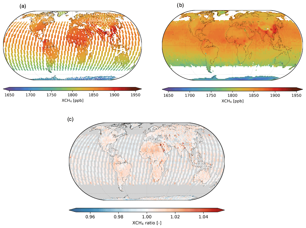
Figure 5Global distribution of XCH4 measured by (a) GOSAT and (b) TROPOMI and (c) the ratio of GOSAT to TROPOMI XCH4. Daily collocations are averaged to a grid for the period 1 March 2018–31 December 2020.
Globally, on average TROPOMI XCH4 underestimates GOSAT XCH4, as shown in Fig. 5c, which depicts the GOSAT-to-TROPOMI XCH4 ratio. Over ocean, the comparison leads to a bias and standard deviation of ppb ( %). Before the correction, the bias over ocean is ppb. Over land, the comparison leads to a bias after correction of ppb ( %) and a Pearson's correlation coefficient of 0.87. The TROPOMI–GOSAT bias for land and ocean measurements is more comparable before applying the correction over the ocean than after. This may be explained by the fact that GOSAT may also have some land–ocean contrast in the XCH4 distribution. As mentioned in Sect. 2.1, the inherent difference in the forward model for land and ocean scenes results in residual differences between XCH4 retrieved over land and over ocean. While the correction applied to TROPOMI XCH4 over the ocean aims to homogenize the XCH4 distribution between land and ocean based solely on TROPOMI data, the correction applied to GOSAT ocean data is based on the validation with four TCCON stations (Buchwitz et al., 2019).
The bias over land is of similar magnitude as before applying the updates to the retrieval algorithm to include ocean measurements (see Sect. 2) (Lorente et al., 2021). The standard deviation of the TROPOMI and GOSAT bias, as well as the station-to-station variability in the TCCON validation (Sect. 4.1), may be used as an estimation of the regional or spatially variable bias to be applied in regional inversions that use TROPOMI XCH4 data (e.g. Varon et al., 2022; Qu et al., 2021).
4.3 Challenging scenes over ocean
Transport of dust towards sea surfaces from the Sahara and other desert areas is challenging for the full-physics retrieval of greenhouse gases. The desert dust particles are aerosols with high optical depth and with optical properties that may differ from the scattering properties assumed in the forward model. Inaccuracies in the modelling of the light path modifications produced by scattering from aerosol particles over the relatively dark ocean surface may result in an underestimation of the retrieved XCH4. This is visible in Fig. 1 on the Atlantic shore of the Sahara desert, as well as in the Red Sea and the Arabian Gulf. The current filtering process for the TROPOMI XCH4 data related to scattering in the atmosphere consists of three steeps. First, we use VIIRS data to compute the cloud fraction based on the scenes classified as confidently and probably clear (Siddans, 2016), and we apply a threshold for the cloud fraction of 0.001. Then, we use the effective aerosol optical thickness (AOT) in the near-infrared spectral band to filter scenes that can be affected by scattering, with a threshold of 0.3. The AOT in the short-wave–infrared can be applied as an equivalent filter with a threshold of 0.1, resulting in a more strict filtering. Finally, as a back-up option in case VIIRS data are not available, we apply a filter based on the differences in the retrieved XCH4 and H2O between the strong and weak absorption bands (Hu et al., 2016).
Figure 6 shows an example of a single orbit where the sun glint area is affected by dust outflow from the Sahara. Figure 6a depicts retrieved XCH4 after applying the VIIRS cloud filter. Figure 6b shows the MODIS-corrected true colour reflectance with the TROPOMI sun glint area outlined in white, where a clear dust outflow event can be seen. The VIIRS data fail to filter out these scenes, as they classify scenes as cloud-free, which does not necessarily imply clear sky. Figure 6c and d show the retrieved effective AOT in the NIR and SWIR spectral bands, with the colour range adjusted to reflect the thresholds of 0.3 and 0.1, respectively. AOT distribution captures the high aerosol load both over land and over ocean. Over the sun glint area, the retrieved AOT captures the gradient of aerosol concentration, with a lower AOT just above 20∘ N latitude. The XCH4 distribution over the sun glint area is directly affected by the aerosols: between 15 and 20∘ N latitude, the aerosol load acts as a highly reflective surface, resulting in a light path enhancement and an overestimation of the retrieved XCH4. In contrast, above 20∘ N latitude, the aerosol load is small compared to other areas, and over the relatively dark ocean scenes, the scattering effect results in a light path shortening and consequently in an underestimation of the retrieved XCH4. Figure 6e and f show the XCH4 distribution after the filter in the NIR AOT (0.3) and SWIR AOT (0.1) has been applied. The NIR AOT filter fails to filter the scenes with the strongest XCH4 underestimation. The SWIR AOT filter is more stringent, but few scenes with a clear XCH4 underestimation still pass the filter.
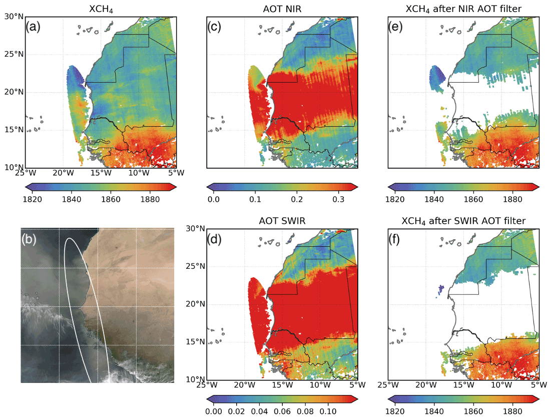
Figure 6Single orbit (no. 7309) over ocean on 12 March 2019. (a) XCH4 only filtered by clouds, (b) MODIS-corrected true colour reflectance, (c) NIR aerosol optical depth, (d) SWIR aerosol optical depth, (e) XCH4 after aerosol filter (AOT NIR >0.3), (f) XCH4 after aerosol filter (AOT SWIR >0.1). XCH4 has been de-striped and corrected for surface reflectance spectral dependencies.
This particular case highlights the difficulties in filtering the TROPOMI XCH4 data when dust outbreaks cover scenes over the ocean, which are the most challenging scenes for the full-physics retrieval algorithm. The filter based on the SWIR AOT is more strict than the NIR AOT; however, over land it is too strict and removes scenes where the retrieved XCH4 is of good quality. Other TROPOMI products like the aerosol layer height (de Graaf et al., 2021) or the aerosol index (Stein Zweers, 2021) do not result in a more accurate filtering than the one based on the parameters from the XCH4 retrieval. The use of other aerosol products from VIIRS for filtering dust events is currently under investigation.
In the TROPOMI XCH4 full-physics retrieval, the oxygen (O2) A-band in the near-infrared spectral region provides part of the information on the full physics scattering properties of the atmosphere. The effect of atmospheric scattering on the O2 A-band has already been discussed in detail in the literature (e.g. Aben et al., 2007). Ignoring atmospheric scattering by aerosols in this spectral band may lead to an under- or overestimation of the atmospheric light path in the forward model simulation, depending on the reflection at the surface and the scattering of light throughout the atmosphere. For glint observations, the ocean surface is only bright for the particular geometry where the specular reflection occurs and dark for all other scattering geometries. This makes atmospheric multiple scattering of sunlight between the surface and the atmosphere unlikely, favouring the shortening of the light path due to single scattering of light by aerosols. Thus, total column O2 retrievals from the O2 A-band ignoring atmospheric scattering by aerosols results in an underestimation of retrieved O2 due to unaccounted shortening of the light path through the atmosphere.
The particular scattering properties of the sun glint observations are the basis for the so-called “upper-edge” method proposed by (Butz et al., 2011, 2013)) to validate GOSAT observations in the O2 A-band. Total column O2 retrievals from the O2 A-band assuming a non-scattering atmosphere can be used to identify scenes over the ocean which are aerosol-free. For this ensemble, the comparison of retrieved O2 to total column O2 concentrations derived from numerical weather prediction models (e.g. ECMWF) provides a validation tool and can be used to investigate sources of error other than light scattering, like spectroscopy uncertainties or instrumental errors. For this purpose, we retrieve O2 total column for sun glint ocean measurements by only accounting for molecular Rayleigh scattering and ignoring scattering by aerosols. We perform the analysis only for scenes that are cloud-free based on measurements from VIIRS. We also apply a filter based on the non-scattering H2O and CH4 retrieval from the weak and strong absorption bands (Hu et al., 2016; Lorente et al., 2021) to remove scenes with clouds not captured by the VIIRS filter.
Figure 7a shows the time series of the weekly distribution of the ratio of retrieved O2 to meteorological O2 from the ECMWF (European Centre for Medium-Range Weather Forecasts) operational atmospheric reanalysis (ERA5) product. For each week, we compute the histogram for ratio bins of 0.002 and normalize it to the maximum number of occurrences such that a value of 1 corresponds to the ratio bin with the highest value of occurrence (red in Fig. 7a). As we retrieve O2 ignoring aerosol scattering effects in the atmosphere, the highest occurrence peak should be below the ratio of 1, which would imply an underestimation of the retrieved O2 due to the unaccounted scattering effects. However, the highest occurrence peak is found close to a ratio of 1.03. The upper edge, which corresponds to scenes free of aerosol scattering effects, is defined as the O2 ratio between the 95th and 99th percentile of the distribution (following the selection criteria by Butz et al., 2013). It is represented in Fig. 7a by the white dots. The statistical selection of the upper edge is supported by the fit quality of the non-scattering O2 retrieval (Fig. 7b), which coincides with a relatively low value of χ2 and low standard error for the upper-edge ensemble. An increase in χ2 and its highest value corresponds to the scenes where scattering processes cannot be ignored, resulting in a poor quality of the fit and an underestimation of the retrieved O2.
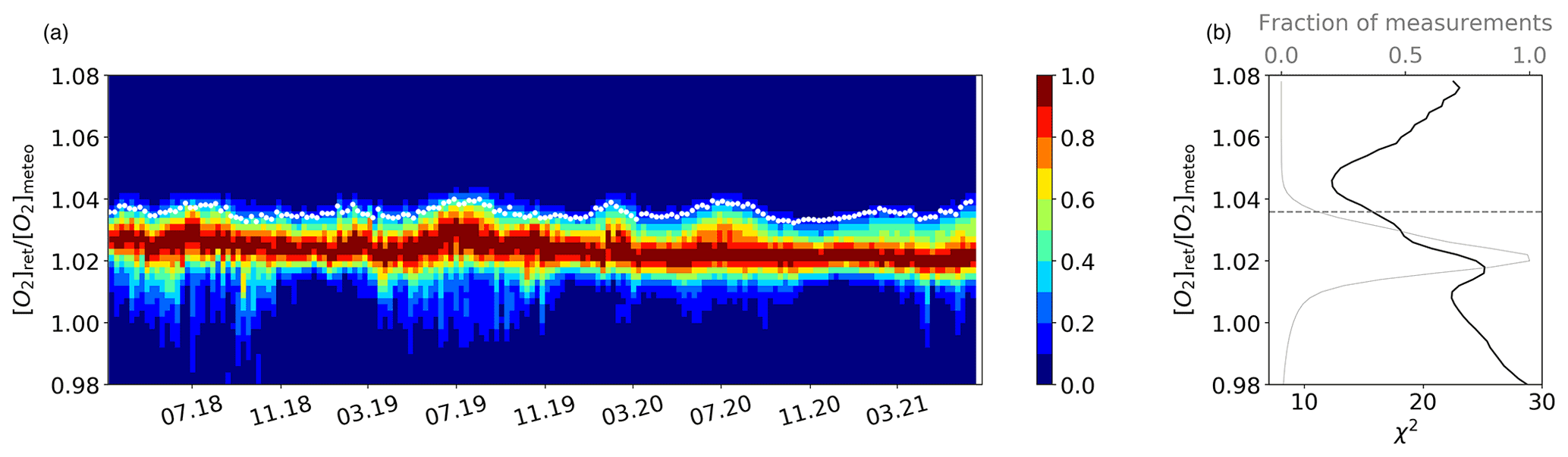
Figure 7(a) Time series of weekly distribution of the ratio of retrieved non-scattering O2 to meteorological (ECMWF) O2. The ratio distribution is normalized such that the maximum occurrence corresponds to the red value 1. White dots are the upper-edge ensemble defined as the scenes between the 95th and 99th percentile of the distribution. (b) Distribution of the ratio as a function of the fitting quality χ2 (black line) and the fraction of measurements for each ratio bin (grey line). The horizontal dashed line corresponds to the upper-edge factor computed as the average over the 3-year period shown in panel (a).
The upper edge should align with the ratio around the value of 1, which would mean that there are no scattering effects in the atmosphere, and thus the non-scattering assumption in the retrieval is valid for these scenes. However, the average over the 3-year period yields a factor of 1.0358 for the upper edge. In March 2020 there was a switch in the VIIRS data used to calculate the cloud fraction for cloud filtering in the XCH4 retrieval (see Sect. 3). Figure 7a shows that after that switch the distribution of the ratio is more uniform and less scattered. Data before March 2020 show a more pronounced lower tail in the distribution, most likely because it contains scenes with some cloud contamination even after applying the filtering. The seasonal pattern throughout the complete time series of the distribution corresponds to the seasonality of the sun glint area (see Appendix A). Between November and March the glint area covers mostly the Southern Hemisphere, and the distribution is narrower. Between March and November the glint area covers mostly the Northern Hemisphere, the lower tail is longer than in other periods, and the upper edge shows a maximum in July. This is true even after the switch in the cloud mask; therefore the seasonality of the upper edge is most probably caused by natural factors like dust outbreaks or residual cloudiness not detected by the filtering. Because of the relatively long time series available, neither the cloud mask switch nor the seasonality of the distribution affects the value of the upper-edge factor.
Previous studies used the same method to evaluate XCO2 and XCH4 full-physics retrieval algorithms applied to GOSAT data (e.g. Butz et al., 2011; Crisp et al., 2012; Yoshida et al., 2013); they all found a value of similar magnitude for the upper-edge factor (1.030, 1.025 and 1.01, respectively), which hints at potential non-instrumental errors with its source in the forward model. All these retrievals differ in the NIR spectral band used, in the forward model and in the definition of the state vector. As the upper-edge ensemble consists of scenes free of scattering errors, the bias in the retrieved surface pressure and O2 in these studies was attributed to an underestimate of the spectroscopic O2 A-band absorption cross-sections such that it was introduced as a constant scaling factor to model the O2 line strengths.
Following this approach, we introduce the upper-edge ensemble factor as a constant scaling factor in the O2 cross-section to model the O2 absorption lines in the forward model and analyse how it affects the TROPOMI XCH4 retrieval. Globally, based on 1 year of data from September 2018 to September 2019, the change in XCH4 is negligible, with an average difference of 0.1±3.7 ppb. The relatively high standard deviation of the differences (compared to the 0.1 ppb average) and a close-to-zero average difference resemble effects of opposite sign found at specific locations and periods. The effect of applying the O2 scaling factor on retrieved XCH4 is relatively more pronounced over high-albedo scenes, like the Sahara desert, and results in enhanced XCH4 when including the O2 cross-section factor. On average over North Africa (15–30∘ N, 20∘ W–35∘ E), retrieved XCH4 is higher by 1.8 ppb (0.1 %), with the highest differences found in January and February, which locally can be up to 12 ppb (0.6 %) (the average for these months is 4 ppb (0.2 %)). Over low-albedo scenes, introducing the O2 scaling factor results in lower retrieved XCH4. On average over high latitudes over the Eurasian region (55–75∘ N, 50–170∘ W) the O2 scaling factor lowers the retrieved XCH4 by 3 ppb (0.15 %) from February to April, with differences that locally can be up to 10 ppb (0.5 %). For SWIR albedo between 0.15 and 0.2 the effect of the O2 factor is smallest, which furthers supports the idea of an albedo range where errors in the quantification of light path modifications are minimum. The effect for both high- and low-albedo scenes is a direct consequence of the enhancement and shortening of the light path by the O2 scaling factor due to the physical effects of scattering in the atmosphere and absorption and reflection on the surface (e.g. Aben et al., 2007). However, in any of the cases the fitting quality in the NIR band shows a clear improvement. The retrieved aerosol optical thickness in the NIR decreases on average from 0.1 to 0.09 when introducing the factor, with local differences that can be up to 0.03 but not necessarily for scenes where differences in XCH4 are the highest. This variable is used as a filtering parameter, but introducing the O2 scaling factor does not significantly change the number of scenes that pass the filter.
These findings show that the effect of the O2 scaling factor on TROPOMI XCH4 retrievals is overall not significant. In the specific cases where the change in retrieved XCH4 is more pronounced, whether it results in an improved retrieval is not supported by the retrieval quality parameters, as it would be for example an improved fit quality. Butz et al. (2011) reported a higher XCH4 by 0.26 % and a slightly bigger change in AOT than our results when the O2 scaling factor was introduced in the GOSAT retrievals. Yoshida et al. (2013) reported an improvement in the bias with TCCON for XCH4 of 10 ppb. This differs from the present analysis, where neither the TCCON validation nor the comparison to XCH4 retrieved from GOSAT measurements captures any of the reported differences. Based on the effects reported in those studies compared to ours, it may be that the O2 A-band has a higher effect on XCH4 for GOSAT than for TROPOMI. In any case, these results suggest a different nature of the bias found when applying the upper-edge method, for which a simple scaling of the O2 line strengths might not be sufficient.
Sensitivity to fitting window
After we have defined the upper-edge ensemble, we investigate the consistency of the retrieved XCH4 for different spectral windows in the short-wave–infrared spectral band for these scenes. Since the upper-edge ensemble should consist of scenes free of scattering effects, we expect good agreement in XCH4 retrieved in the different fitting windows. To investigate this, we process 3 months of data (March–May 2020, around 43 500 scenes after filtering) for several fitting windows (see Table 4) using a non-scattering version of the RemoTeC retrieval algorithm which ignores both Rayleigh and particle scattering in the atmosphere. As Rayleigh scattering is stronger for shorter wavelengths, the effect in the 2.3 µm band can be ignored.
Table 4Spectral fitting windows used in the non-scattering XCH4 retrieval for the upper-edge ensemble and the bias and standard deviation of the differences in the retrieved XCH4 with respect to the original fitting window W0.
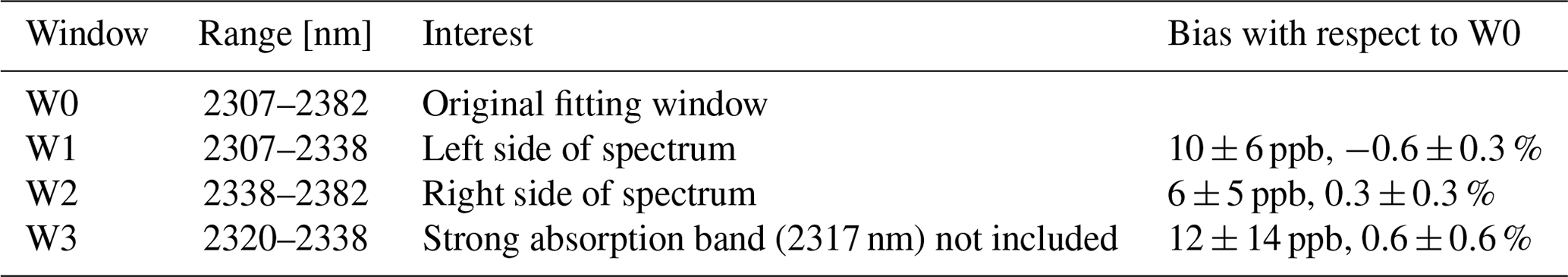
The agreement in the retrieved XCH4 for the various windows with respect to the original fitting window is on average within 0.6 %. The bias and standard deviation of the differences are summarized in the last column of Table 4. The bias for the spectral window W1, which contains only the left side of the spectrum, is negative, so retrieved XCH4 is lower (−0.6 %, −10 ppb), while for W2, which contains the right side of the spectrum, it is positive and smaller in magnitude (0.3 %, 6 ppb). These results are likely to be related to the different relative strength of the absorption bands that each of the fitting windows includes. For the spectral window W3, which ignores the strong absorption band at 2317 nm, the bias is positive (0.6 %, 12 ppb) and similar in magnitude as for W1.
The differences in the retrieved XCH4 for the different fitting windows are relatively small, but since these are presumably scenes free of aerosol scattering effects, we further investigate the possible sources of error that lead to such differences. For W1 and W2, the scatter in the differences is of the same magnitude as the bias or smaller; for W3 the scatter is largest in magnitude compared to W1 and W2 and slightly larger than the bias, and the effect of the measurement noise on the retrieval is also highest (not shown). This could be explained by the upper-edge ensemble containing scenes with residual scattering effects, which could affect more the narrower window that does not include the strong CH4 absorption band. Another possible error source is the absorption line strengths and line shapes. The spectroscopy database for the absorption cross-section used in the retrieval is the Scientific Exploitation of Operational Missions – Improved Atmospheric Spectroscopy Database (SEOM-IAS) (Birk et al., 2017). The agreement between the different fitting windows did not improve when substituting the absorption cross-section database by HITRAN 2008: the effect was to add an overall positive bias in the retrieved XCH4, similar to what was found in Lorente et al. (2021). The evaluation of the quality of the spectral fit for the different windows also did not point to errors related to the calibration of the absorption lines. We also investigated the possibility of radiometric inaccuracies by fitting an intensity-dependent offset, which could not explain the difference in XCH4 we observed.
We have retrieved 4 years of XCH4 from TROPOMI measurements over the ocean for sun glint geometries, enhancing the monitoring capabilities for methane with their addition to retrievals over land that have been available since October 2017. We have optimized the S5P-RemoTeC full-physics retrieval algorithm for the specific information content on atmospheric scattering available from ocean measurements, where direct solar scattering from surface reflection dominates over the diffuse contribution. Furthermore, the forward model has inherent differences on how land and ocean surface reflection is modelled. This results in residual differences between XCH4 retrieved over land and ocean, so in order to homogenize the XCH4 distribution we have derived a constant correction factor for ocean retrievals independent of the retrieved parameters and based only on TROPOMI data. The TROPOMI global mean XCH4 shows an annual increase with respect to the previous year of 7.3, 10.6 and 15 ppb in 2019, 2020 and 2021, respectively, a tendency of increase in the growth rate that is also captured by surface measurements.
The specular reflection of water surfaces in the specific sun glint geometry results in a measured reflectance from which methane can be retrieved with an accuracy and precision within the mission requirements. The validation with measurements from the ground-based TCCON sites from islands and near-coast sites results in a bias and station-to-station variability of % ( ppb), and the comparison to ocean measurements from the GOSAT results in a bias of % ( ppb). Based on the magnitude of the bias, station-to-station variability and standard deviation for land and ocean retrievals, we can conclude that the data over land and ocean have a similar data quality.
Ocean measurements over sun glint geometry provide an opportunity to further validate XCH4 retrievals. The specific atmospheric scattering properties and reflection from water surfaces allow the upper-edge method to be applied to the O2 A-band. The method rests on the principle that over ocean, scattering processes always lead to an underestimation of the retrieved O2 if light path shortening due to aerosol scattering processes is not taken into account. We use O2 retrievals from the O2 A-band to evaluate the forward model by comparing the retrieved O2 to meteorological O2. Based on the upper-edge method we created a diagnostic dataset composed of scenes where scattering effects due to clouds and aerosols can be neglected such that it can be used to investigate sources of error other than approximations of scattering processes in the forward model. The ratio for these scenes free of aerosol scattering should align around the value of 1; however we find a bias of 1.04. The magnitude of this bias is similar to what previous studies found when applying the upper-edge method to GOSAT, which hints at potential non-instrumental errors. The hypothesis was that this bias may have its source in the forward model such that the upper-edge factor was introduced as a constant scaling factor in the O2 absorption line strengths. By doing so in the TROPOMI XCH4 retrievals, we conclude that the effect on XCH4 is overall not significant and that the sign and magnitude of the effect depends on surface albedo. Moreover, neither TCCON validation nor the comparison to XCH4 retrieved from GOSAT captures any of the differences in retrieved XCH4 after applying the O2 scaling factor. These results suggest a different nature of the bias found when applying the upper-edge method, for which a simple scaling of the O2 line strengths might not be sufficient. It also suggests that TROPOMI XCH4 retrievals from the 2.3 µm are less affected by inaccuracies affecting the O2 band than retrievals using the 1.6 µm band.
We have further used the upper-edge ensemble to investigate the consistency of the retrieved XCH4 for different spectral windows in the short-wave–infrared spectral band using a non-scattering version of the RemoTeC retrieval algorithm. The agreement in the retrieved XCH4 for the various windows with respect to the original fitting window is 0.8 % on average, a consistency within the precision and accuracy requirements of the mission. The different biases for the different windows are likely to be related to the different relative strength of the absorption bands that each of the fitting windows includes. The scatter of the differences is in all cases similar to or higher than the bias, which could be because the upper edge may contain scenes with residual scattering effects. The evaluation of the quality of the spectral fit for the different windows did not point to errors related to the calibration of the absorption lines, and we could not identify any radiometric inaccuracies.
The sun glint angle is defined as
where θo and θ are the solar and viewing zenith angle, respectively, and ϕo and ϕ are the solar and viewing azimuth angles, respectively. The dependency of the angle on the solar position results in a seasonal cycle on the coverage; i.e. different latitudinal ranges are covered throughout the year, as shown by the orbits plotted for different months in Fig. A1. Each glint area in the figure corresponds to one orbit for a specific month and day of the year. In a specific orbit, the sun glint area is defined such that the sun glint angle is lower than 20∘. The signal measured over the ocean in scenes with low α (e.g. from 0 to 5∘) can be twice as high as that measured at the edges (e.g. for α=20∘). For values higher than 20∘, the signal is too low, and the noise dominates such that XCH4 cannot be retrieved with enough precision and accuracy.
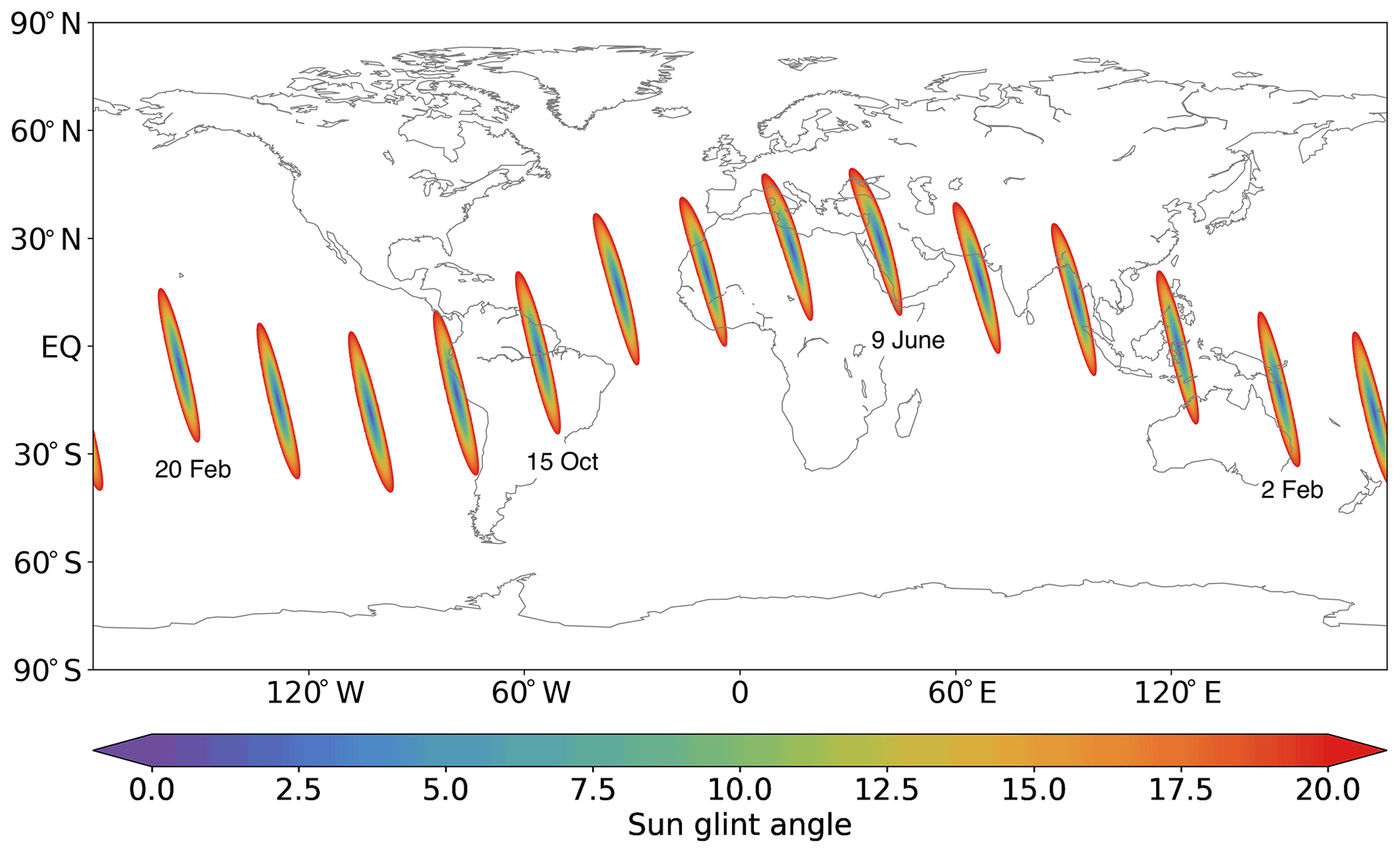
Figure A1Sun glint angle seasonal cycle. Each coloured area corresponds to the sun glint area (i.e. SGA <20∘) for separate orbits in different months throughout the year, starting 1 January on the easternmost orbit and increasing months towards the west.
Here we summarize the geolocation of the TCCON ground-based stations used for validation of TROPOMI XCH4 data in Sect. 4.
Velazco et al. (2017)Blumenstock et al. (2014)De Mazière et al. (2014)Morino et al. (2016b)Morino et al. (2016a)Wennberg et al. (2017b)Iraci et al. (2016)Kawakami et al. (2017)Griffith et al. (2017a)Griffith et al. (2017b)Table B1Overview of the stations from the TCCON network used for validation of ocean sun glint measurements in Sect. 4.1.1.
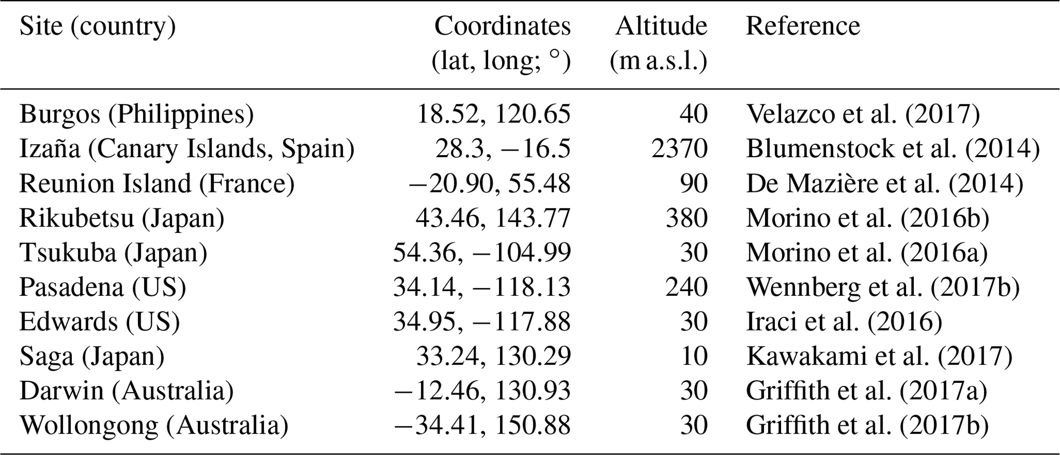
Table B2Overview of the stations from the TCCON network used for validation of land measurements in Sect. 4.1.2.

* For the Lauder station the ll instrument was replaced in October 2018 to lr.
The SRON S5P-RemoTeC scientific TROPOMI XCH4 dataset from this study is available for download at https://zenodo.org/record/7303388 or at https://ftp.sron.nl/open-access-data-2/TROPOMI/tropomi/ch4/18_17/ (last access: 8 November 2022) (Lorente et al., 2022). This corresponds to the scientific SRON S5P RemoTeC TROPOMI XCH4 product, which was processed as the pre-operational version of the operational TROPOMI XCH4 retrieval. Measurements over ocean under sun glint geometry with the retrieval settings presented in this paper were activated in the operational processing in November 2021, under version 2.3.0.
AL, TB, MCV, OH, AB and JL provided the TROPOMI CH4 retrieval and data analysis. AL wrote the original draft with input from TB and JL. All authors discussed the results and reviewed and edited the paper.
At least one of the (co-)authors is a member of the editorial board of Atmospheric Measurement Techniques. The peer-review process was guided by an independent editor, and the authors also have no other competing interests to declare.
The presented work has been performed in the frame of Sentinel-5 Precursor Validation Team (S5PVT) or Level 1/Level 2 Product Working Group activities. Results are based on preliminary (not fully calibrated or validated) Sentinel-5 precursor data that will still change. The results are based on S5P L1B version 1 data. Plots and data contain modified Copernicus Sentinel data, processed by SRON.
Publisher’s note: Copernicus Publications remains neutral with regard to jurisdictional claims in published maps and institutional affiliations.
The TROPOMI data processing was carried out with the Dutch National e-infrastructure with the support of the SURF cooperative.
This research has been supported by the TROPOMI national programme from the NSO and Methane+.
This paper was edited by Helen Worden and reviewed by two anonymous referees.
Aben, I., Hasekamp, O., and Hartmann, W.: Uncertainties in the space-based measurements of CO2 columns due to scattering in the Earth's atmosphere, J. Quant. Spectrosc. Ra., 104, 450–459, https://doi.org/10.1016/j.jqsrt.2006.09.013, 2007. a, b, c, d
Birk, M., Wagner, G., Loos, J., Wilzewski, J., Mondelain, D., Campargue, A., Hase, F., Orphal, J., Perrin, A., Tran, H., Daumont, L., Rotger-Languereau, M., Bigazzi, A., and Zehner, C.: Methane and water spectroscopic database for TROPOMI Sentinel 5 Precursor in the 2.3 µm region, EGU General Assembly, Vienna, Austria, 23–28 April 2017, EGU2017-14652, 2017. a
Blumenstock, T., Hase, F., Schneider, M., García, O. E., and Sepúlveda, E.: TCCON data from Izana (ES), Release GGG2014.R0, CaltechDATA [data set], https://doi.org/10.14291/TCCON.GGG2014.IZANA01.R0/1149295, 2014. a
Buchwitz, M., Reuter, M., Schneising, O., Hewson, W., Detmers, R. G., Boesch, H., Hasekamp, O., Aben, I., Bovensmann, H., Burrows, J., Butz, A., Chevallier, F., Dils, B., Frankenberg, C., Heymann, J., Lichtenberg, G., De Mazière, M., Notholt, J., Parker, R., Warneke, T., Zehner, C., Griffith, D. W. T., Deutscher, N., Kuze, A., Suto, H., and Wunch, D.: Global satellite observations of column-averaged carbon dioxide and methane: The GHG-CCI XCO2 and XCH4 CRDP3 data set, Remote Sens. Environ., 203, 276–295, https://doi.org/10.1016/j.rse.2016.12.027, 2017. a
Buchwitz, M., Aben, I., Armante, R., Boesch, H., Crevoisier, C., Di Noia, A., Hasekamp, O. P., Reuter, M., Schneising-Weigel, O., and Wu, L.: Algorithm Theoretical Basis Document (ATBD) – Main document for Greenhouse Gas (GHG: CO2 and CH4) data set CDR 3 (2003–2018), C3S project, Copernicus Climate Change Service, Project number: C3S_D312b_Lot2.1.3.2-v1.0_ATBD-GHG_MAIN_v3.1, 43 pp., https://www.iup.uni-bremen.de/carbon_ghg/docs/C3S/CDR3_2003-2018/ATBD/C3S_D312b_Lot2.1.3.2-v1.0_ATBD-GHG_MAIN_v3.1.pdf (last access: 8 November 2022), 2019. a, b
Butz, A., Hasekamp, O. P., Frankenberg, C., Vidot, J., and Aben, I.: CH4 retrievals from space-based solar backscatter measurements: Performance evaluation against simulated aerosol and cirrus loaded scenes, J. Geophys. Res., 115, D24302, https://doi.org/10.1029/2010JD014514, 2010. a
Butz, A., Guerlet, S., Hasekamp, O., Schepers, D., Galli, A., Aben, I., Frankenberg, C., Hartmann, J.-M., Tran, H., Kuze, A., Keppel-Aleks, G., Toon, G., Wunch, D., Wennberg, P., Deutscher, N., Griffith, D., Macatangay, R., Messerschmidt, J., Notholt, J., and Warneke, T.: Toward accurate CO2 and CH4 observations from GOSAT, Geophys. Res. Lett., 38, L14812, https://doi.org/10.1029/2011GL047888, 2011. a, b, c, d, e
Butz, A., Guerlet, S., Hasekamp, O. P., Kuze, A., and Suto, H.: Using ocean-glint scattered sunlight as a diagnostic tool for satellite remote sensing of greenhouse gases, Atmos. Meas. Tech., 6, 2509–2520, https://doi.org/10.5194/amt-6-2509-2013, 2013. a, b, c, d
Cogan, A. J., Boesch, H., Parker, R. J., Feng, L., Palmer, P. I., Blavier, J.-F. L., Deutscher, N. M., Macatangay, R., Notholt, J., Roehl, C., Warneke, T., and Wunch, D.: Atmospheric carbon dioxide retrieved from the Greenhouse gases Observing SATellite (GOSAT): Comparison with ground-based TCCON observations and GEOS-Chem model calculations, J. Geophys. Res., 117, D21301, https://doi.org/10.1029/2012JD018087, 2012. a
Cox, C. and Munk, W.: Measurement of the Roughness of the Sea Surface from Photographs of the Sun's Glitter, J. Opt. Soc. Am., 44, 838–850, https://doi.org/10.1364/JOSA.44.000838, 1954. a
Crisp, D., Fisher, B. M., O'Dell, C., Frankenberg, C., Basilio, R., Bösch, H., Brown, L. R., Castano, R., Connor, B., Deutscher, N. M., Eldering, A., Griffith, D., Gunson, M., Kuze, A., Mandrake, L., McDuffie, J., Messerschmidt, J., Miller, C. E., Morino, I., Natraj, V., Notholt, J., O'Brien, D. M., Oyafuso, F., Polonsky, I., Robinson, J., Salawitch, R., Sherlock, V., Smyth, M., Suto, H., Taylor, T. E., Thompson, D. R., Wennberg, P. O., Wunch, D., and Yung, Y. L.: The ACOS CO2 retrieval algorithm – Part II: Global X data characterization, Atmos. Meas. Tech., 5, 687–707, https://doi.org/10.5194/amt-5-687-2012, 2012. a, b
de Graaf, M., de Haan, J. F., and Sanders, A.: Algorithm Theoretical Baseline Document of the Aerosol Layer Height, KNMI, De Bilt, The Netherlands, Report Number: S5P-KNMI-L2-0006-RP, version 2.4.0, https://sentinel.esa.int/documents/247904/2476257/Sentinel-5P-TROPOMI-ATBD-Aerosol-Height (last access: 8 November 2022), 2021. a
De Mazière, M., Sha, M. K., Desmet, F., Hermans, C., Scolas, F., Kumps, N., Metzger, J.-M., Duflot, V., and Cammas, J.-P.: TCCON data from Réunion Island (RE), Release GGG2014.R0, CaltechDATA [data set], https://doi.org/10.14291/tccon.ggg2014.reunion01.R0/1149288, 2014. a
Griffith, D. W. T., Deutscher, N. M., Velazco, V. A., Wennberg, P. O., Yavin, Y., Keppel-Aleks, G., Washenfelder, R. A., Toon, G. C., Blavier, J.-F., Paton-Walsh, C., Jones, N. B., Kettlewell, G. C., Connor, B. J., Macatangay, R. C., Roehl, C., Ryczek, M., Glowacki, J., Culgan, T., and Bryant, G. W.: TCCON data from Darwin (AU), Release GGG2014.R0, CaltechDATA [data set], https://doi.org/10.14291/tccon.ggg2014.darwin01.r0/1149290, 2017a. a, b
Griffith, D. W. T., Velazco, V. A., Deutscher, N. M., Paton-Walsh, C., Jones, N. B., Wilson, S. R., Macatangay, R. C., Kettlewell, G. C., Buchholz, R. R., and Riggenbach, M.: TCCON data from Wollongong (AU), Release GGG2014.R0, CaltechDATA [data set], https://doi.org/10.14291/tccon.ggg2014.wollongong01.r0/1149291, 2017b. a, b
Guerlet, S., Butz, A., Schepers, D., Basu, S., Hasekamp, O. P., Kuze, A., Yokota, T., Blavier, J., Deutscher, N. M., Griffith, D. W., Hase, F., Kyro, E., Morino, I., Sherlock, V., Sussmann, R., Galli, A., and Aben, I.: Impact of aerosol and thin cirrus on retrieving and validating XCO2 from GOSAT shortwave infrared measurements, J. Geophys. Res.-Atmos., 118, 4887–4905, https://doi.org/10.1002/jgrd.50332, 2013. a
Hase, F., Blumenstock, T., Dohe, S., Groß, J., and Kiel, M.: TCCON data from Karlsruhe (DE), Release GGG2014.R0, CaltechDATA [data set], https://doi.org/10.14291/tccon.ggg2014.karlsruhe01.r0/1149270, 2017. a
Hasekamp, O., Lorente, A., Hu, H., Butz, A., aan de Brugh, J., and Landgraf, J.: Algorithm Theoretical Baseline Document for Sentinel-5 Precursor methane retrieval, KNMI, De Bilt, The Netherlands, Document number: SRON-S5P-LEV2-RP-001, version 2.4.0, https://sentinels.copernicus.eu/documents/247904/2476257/Sentinel-5P-TROPOMI-ATBD-Methane-retrieval.pdf (last access: 8 November 2022), 2021. a
Houweling, S., Hartmann, W., Aben, I., Schrijver, H., Skidmore, J., Roelofs, G.-J., and Breon, F.-M.: Evidence of systematic errors in SCIAMACHY-observed CO2 due to aerosols, Atmos. Chem. Phys., 5, 3003–3013, https://doi.org/10.5194/acp-5-3003-2005, 2005. a
Hu, H., Hasekamp, O., Butz, A., Galli, A., Landgraf, J., Aan de Brugh, J., Borsdorff, T., Scheepmaker, R., and Aben, I.: The operational methane retrieval algorithm for TROPOMI, Atmos. Meas. Tech., 9, 5423–5440, https://doi.org/10.5194/amt-9-5423-2016, 2016. a, b, c, d, e
Iraci, L. T., Podolske, J. R., Hillyard, P. W., Roehl, C., Wennberg, P. O., Blavier, J.-F., Landeros, J., Allen, N., Wunch, D., Zavaleta, J., Quigley, E., Osterman, G. B., Albertson, R., Dunwoody, K., and Boyden, H.: TCCON data from Edwards (US), Release GGG2014.R1, CaltechDATA [data set], https://doi.org/10.14291/TCCON.GGG2014.EDWARDS01.R1/1255068, 2016. a, b
Irakulis-Loitxate, I., Guanter, L., Maasakkers, J. D., Zavala-Araiza, D., and Aben, I.: Satellites Detect Abatable Super-Emissions in One of the World's Largest Methane Hotspot Regions, Environ. Sci. Technol., 56, 2143–2152, 2022. a
Kawakami, S., Ohyama, H., Arai, K., Okumura, H., Taura, C., Fukamachi, T., and Sakashita, M.: TCCON data from Saga (JP), Release GGG2014.R0, CaltechDATA [data set], https://doi.org/10.14291/tccon.ggg2014.saga01.r0/1149283, 2017. a, b
Kivi, R. and Heikkinen, P.: Fourier transform spectrometer measurements of column CO2 at Sodankylä, Finland, Geosci. Instrum. Method. Data Syst., 5, 271–279, https://doi.org/10.5194/gi-5-271-2016, 2016. a
Kivi, R., Heikkinen, P., and Kyrö, E.: TCCON data from Sodankylä (FI), Release GGG2014.R0, CaltechDATA [data set], https://doi.org/10.14291/tccon.ggg2014.sodankyla01.r0/1149280, 2017. a
Landgraf, J., Hasekamp, O. P., Box, M. A., and Trautmann, T.: A linearized radiative transfer model for ozone profile retrieval using the analytical forward-adjoint perturbation theory approach, J. Geophys. Res., 106, 27291–27305, https://doi.org/10.1029/2001JD000636, 2001. a
Lorente, A., Borsdorff, T., Butz, A., Hasekamp, O., aan de Brugh, J., Schneider, A., Wu, L., Hase, F., Kivi, R., Wunch, D., Pollard, D. F., Shiomi, K., Deutscher, N. M., Velazco, V. A., Roehl, C. M., Wennberg, P. O., Warneke, T., and Landgraf, J.: Methane retrieved from TROPOMI: improvement of the data product and validation of the first 2 years of measurements, Atmos. Meas. Tech., 14, 665–684, https://doi.org/10.5194/amt-14-665-2021, 2021. a, b, c, d, e, f, g, h, i, j
Lorente, A., Borsdorff, T., Martinez Velarte, M. C., and Landgraf, J.: SRON S5P – RemoTeC scientific TROPOMI XCH4 dataset v18_17, Zenodo [data set], https://doi.org/10.5281/zenodo.7303388, 2022 (data also available at: https://ftp.sron.nl/open-access-data-2/TROPOMI/tropomi/ch4/18_17/, last access: 8 November 2022). a
Morino, I., Matsuzaki, T., and Horikawa, M.: TCCON data from Tsukuba (JP), 125HR, Release GGG2014.R1, CaltechDATA [data set], https://doi.org/10.14291/TCCON.GGG2014.TSUKUBA02.R1/1241486, 2016a. a
Morino, I., Yokozeki, N., Matsuzaki, T., and Horikawa, M.: TCCON data from Rikubetsu (JP), Release GGG2014.R1, CaltechDATA [data set], https://doi.org/10.14291/TCCON.GGG2014.RIKUBETSU01.R1/1242265, 2016b. a
O'Dell, C. W., Eldering, A., Wennberg, P. O., Crisp, D., Gunson, M. R., Fisher, B., Frankenberg, C., Kiel, M., Lindqvist, H., Mandrake, L., Merrelli, A., Natraj, V., Nelson, R. R., Osterman, G. B., Payne, V. H., Taylor, T. E., Wunch, D., Drouin, B. J., Oyafuso, F., Chang, A., McDuffie, J., Smyth, M., Baker, D. F., Basu, S., Chevallier, F., Crowell, S. M. R., Feng, L., Palmer, P. I., Dubey, M., García, O. E., Griffith, D. W. T., Hase, F., Iraci, L. T., Kivi, R., Morino, I., Notholt, J., Ohyama, H., Petri, C., Roehl, C. M., Sha, M. K., Strong, K., Sussmann, R., Te, Y., Uchino, O., and Velazco, V. A.: Improved retrievals of carbon dioxide from Orbiting Carbon Observatory-2 with the version 8 ACOS algorithm, Atmos. Meas. Tech., 11, 6539–6576, https://doi.org/10.5194/amt-11-6539-2018, 2018. a
Pollard, D. F., Robinson, J., and Shiona, H.: TCCON data from Lauder (NZ), Release GGG2014.R0, CaltechDATA [data set], https://doi.org/10.14291/TCCON.GGG2014.LAUDER03.R0, 2019. a
Qu, Z., Jacob, D. J., Shen, L., Lu, X., Zhang, Y., Scarpelli, T. R., Nesser, H., Sulprizio, M. P., Maasakkers, J. D., Bloom, A. A., Worden, J. R., Parker, R. J., and Delgado, A. L.: Global distribution of methane emissions: a comparative inverse analysis of observations from the TROPOMI and GOSAT satellite instruments, Atmos. Chem. Phys., 21, 14159–14175, https://doi.org/10.5194/acp-21-14159-2021, 2021. a
Schepers, D., aan de Brugh, J., Hahne, P., Butz, A., Hasekamp, O., and Landgraf, J.: LINTRAN v2.0: A linearised vector radiative transfer model for efficient simulation of satellite-born nadir-viewing reflection measurements of cloudy atmospheres, J. Quant. Spectrosc. Ra., 149, 347–359, https://doi.org/10.1016/j.jqsrt.2014.08.019, 2014. a
Sha, M. K., Langerock, B., Blavier, J.-F. L., Blumenstock, T., Borsdorff, T., Buschmann, M., Dehn, A., De Mazière, M., Deutscher, N. M., Feist, D. G., García, O. E., Griffith, D. W. T., Grutter, M., Hannigan, J. W., Hase, F., Heikkinen, P., Hermans, C., Iraci, L. T., Jeseck, P., Jones, N., Kivi, R., Kumps, N., Landgraf, J., Lorente, A., Mahieu, E., Makarova, M. V., Mellqvist, J., Metzger, J.-M., Morino, I., Nagahama, T., Notholt, J., Ohyama, H., Ortega, I., Palm, M., Petri, C., Pollard, D. F., Rettinger, M., Robinson, J., Roche, S., Roehl, C. M., Röhling, A. N., Rousogenous, C., Schneider, M., Shiomi, K., Smale, D., Stremme, W., Strong, K., Sussmann, R., Té, Y., Uchino, O., Velazco, V. A., Vigouroux, C., Vrekoussis, M., Wang, P., Warneke, T., Wizenberg, T., Wunch, D., Yamanouchi, S., Yang, Y., and Zhou, M.: Validation of methane and carbon monoxide from Sentinel-5 Precursor using TCCON and NDACC-IRWG stations, Atmos. Meas. Tech., 14, 6249–6304, https://doi.org/10.5194/amt-14-6249-2021, 2021. a
Sherlock, V., Connor, B., Robinson, J., Shiona, H., Smale, D., and Pollard, D. F.: TCCON data from Lauder (NZ), 125HR, Release GGG2014.R0, CaltechDATA [data set], https://doi.org/10.14291/tccon.ggg2014.lauder02.r0/1149298, 2017. a
Siddans, R.: Algorithm Theoretical Baseline Document for S5P-NPP Cloud Processor, RAL Space, Document number: S5P-NPPC-RAL-ATBD-0001, https://sentinel.esa.int/documents/247904/2476257/Sentinel-5P-NPP-ATBD-NPP-Clouds (last access: 8 November 2022), 2016. a
Stein Zweers, D. C.: Algorithm Theoretical Baseline Document if the UV Aerosol Index, KNMI, De Bilt, The Netherlands, Document number: S5P-KNMI-L2-0008-RP, https://sentinel.esa.int/documents/247904/2476257/Sentinel-5P-TROPOMI-ATBD-UV-Aerosol-Index.pdf (last access: 8 November 2022), 2021. a
Varon, D. J., McKeever, J., Jervis, D., Maasakkers, J. D., Pandey, S., Houweling, S., Aben, I., Scarpelli, T., and Jacob, D. J.: Satellite Discovery of Anomalously Large Methane Point Sources From Oil/Gas Production, Geophys. Res. Lett., 46, 13507–13516, https://doi.org/10.1029/2019GL083798, 2019. a
Varon, D. J., Jacob, D. J., Sulprizio, M., Estrada, L. A., Downs, W. B., Shen, L., Hancock, S. E., Nesser, H., Qu, Z., Penn, E., Chen, Z., Lu, X., Lorente, A., Tewari, A., and Randles, C. A.: Integrated Methane Inversion (IMI 1.0): a user-friendly, cloud-based facility for inferring high-resolution methane emissions from TROPOMI satellite observations, Geosci. Model Dev., 15, 5787–5805, https://doi.org/10.5194/gmd-15-5787-2022, 2022. a
Velazco, V. A., Morino, I., Uchino, O., Hori, A., Kiel, M., Bukosa, B., Deutscher, N. M., Sakai, T., Nagai, T., Bagtasa, G., Izumi, T., Yoshida, Y., and Griffith, D. W. T.: TCCON Philippines: First Measurement Results, Satellite Data and Model Comparisons in Southeast Asia, Remote Sens., 9, 1228, https://doi.org/10.3390/rs9121228, 2017. a
Warneke, T., Messerschmidt, J., Notholt, J., Weinzierl, C., Deutscher, N. M., Petri, C., and Grupe, P.: TCCON data from Orléans (FR), Release GGG2014.R0, CaltechDATA [data set], https://doi.org/10.14291/tccon.ggg2014.orleans01.r0/1149276, 2017. a
Wennberg, P. O., Roehl, C. M., Wunch, D., Toon, G. C., Blavier, J.-F., Washenfelder, R., Keppel-Aleks, G., Allen, N. T., and Ayers, J.: TCCON data from Park Falls (US), Release GGG2014.R1, CaltechDATA [data set], https://doi.org/10.14291/tccon.ggg2014.parkfalls01.r1, 2017a. a
Wennberg, P. O., Wunch, D., Roehl, C. M., Blavier, J.-F., Toon, G. C., and Allen, N. T.: TCCON data from Caltech (US), Release GGG2014.R0, CaltechDATA [data set], https://doi.org/10.14291/tccon.ggg2014.pasadena01.r0/1149162, 2017b. a, b
Wennberg, P. O., Wunch, D., Roehl, C. M., Blavier, J.-F., Toon, G. C., and Allen, N. T.: TCCON data from Lamont (US), Release GGG2014.R1, CaltechDATA [data set], https://doi.org/10.14291/tccon.ggg2014.lamont01.r1/1255070, 2017c. a
Wu, L., Hasekamp, O., Hu, H., Landgraf, J., Butz, A., aan de Brugh, J., Aben, I., Pollard, D. F., Griffith, D. W. T., Feist, D. G., Koshelev, D., Hase, F., Toon, G. C., Ohyama, H., Morino, I., Notholt, J., Shiomi, K., Iraci, L., Schneider, M., de Mazière, M., Sussmann, R., Kivi, R., Warneke, T., Goo, T.-Y., and Té, Y.: Carbon dioxide retrieval from OCO-2 satellite observations using the RemoTeC algorithm and validation with TCCON measurements, Atmos. Meas. Tech., 11, 3111–3130, https://doi.org/10.5194/amt-11-3111-2018, 2018. a
Wu, L., aan de Brugh, J., Meijer, Y., Sierk, B., Hasekamp, O., Butz, A., and Landgraf, J.: XCO2 observations using satellite measurements with moderate spectral resolution: investigation using GOSAT and OCO-2 measurements, Atmos. Meas. Tech., 13, 713–729, https://doi.org/10.5194/amt-13-713-2020, 2020. a
Wunch, D., Toon, G. C., Blavier, J.-F. L., Washenfelder, R. A., Notholt, J., Connor, B. J., Griffith, D. W. T., Sherlock, V., and Wennberg, P. O.: The Total Carbon Column Observing Network, Philos. T. Roy. Soc. A, 369, 2087–2112, https://doi.org/10.1098/rsta.2010.0240, 2011. a
Wunch, D., Mendonca, J., Colebatch, O., Allen, N. T., Blavier, J.-F., Roche, S., Hedelius, J., Neufeld, G., Springett, S., Worthy, D., Kessler, R., and Strong, K.: TCCON data from East Trout Lake, SK (CA), Release GGG2014.R1, CaltechDATA [data set], https://doi.org/10.14291/tccon.ggg2014.easttroutlake01.r1, 2017. a
Yoshida, Y., Kikuchi, N., Morino, I., Uchino, O., Oshchepkov, S., Bril, A., Saeki, T., Schutgens, N., Toon, G. C., Wunch, D., Roehl, C. M., Wennberg, P. O., Griffith, D. W. T., Deutscher, N. M., Warneke, T., Notholt, J., Robinson, J., Sherlock, V., Connor, B., Rettinger, M., Sussmann, R., Ahonen, P., Heikkinen, P., Kyrö, E., Mendonca, J., Strong, K., Hase, F., Dohe, S., and Yokota, T.: Improvement of the retrieval algorithm for GOSAT SWIR XCO2 and XCH4 and their validation using TCCON data, Atmos. Meas. Tech., 6, 1533–1547, https://doi.org/10.5194/amt-6-1533-2013, 2013. a, b, c, d
Zhou, M., Dils, B., Wang, P., Detmers, R., Yoshida, Y., O'Dell, C. W., Feist, D. G., Velazco, V. A., Schneider, M., and De Mazière, M.: Validation of TANSO-FTS/GOSAT XCO2 and XCH4 glint mode retrievals using TCCON data from near-ocean sites, Atmos. Meas. Tech., 9, 1415–1430, https://doi.org/10.5194/amt-9-1415-2016, 2016. a
- Abstract
- Introduction
- Retrieval algorithm
- Retrieval results
- Quality assessment
- Upper-edge analysis
- Summary and conclusions
- Appendix A: Sun glint measurement geometry
- Appendix B: TCCON stations used for validation over land and ocean
- Data availability
- Author contributions
- Competing interests
- Disclaimer
- Acknowledgements
- Financial support
- Review statement
- References