the Creative Commons Attribution 4.0 License.
the Creative Commons Attribution 4.0 License.
 | 21 Nov 2022
A CO2-independent cloud mask from Infrared Atmospheric Sounding Interferometer (IASI) radiances for climate applications
Simon Whitburn
Lieven Clarisse
Marc Crapeau
Thomas August
Tim Hultberg
Pierre François Coheur
Cathy Clerbaux
With more than 15 years of continuous and consistent measurements, the Infrared Atmospheric Sounding Interferometer (IASI) radiance dataset is becoming a reference climate data record. To be exploited to its full potential, it requires a cloud filter that is accurate, unbiased over the full IASI life span and strict enough to be used in satellite data retrieval schemes. Here, we present a new cloud detection algorithm which combines (1) a high sensitivity, (2) a good consistency over the whole IASI time series and between the different copies of the instrument flying on board the suite of Metop satellites, and (3) simplicity in its parametrization. The method is based on a supervised neural network (NN) and relies, as input parameters, on the IASI radiance measurements only. The robustness of the cloud mask over time is ensured in particular by avoiding the IASI channels that are influenced by CO2, N2O, CH4, CFC-11 and CFC-12 absorption lines and those corresponding to the ν2 H2O absorption band. As a reference dataset for the training, version 6.5 of the operational IASI Level 2 (L2) cloud product is used. We provide different illustrations of the NN cloud product, including comparisons with other existing products. We find very good agreement overall with version 6.5 of the operational IASI L2 with an identical mean annual cloud amount and a pixel-by-pixel correspondence of about 87 %. The comparison with the other cloud products shows a good correspondence in the main cloud regimes but with sometimes large differences in the mean cloud amount (up to 10 %) due to the specificities of each of the different products. We also show the good capability of the NN product to differentiate clouds from dust plumes.
- Article
(29705 KB) - Full-text XML
-
Supplement
(313 KB) - BibTeX
- EndNote


Clouds cover between 70 % and 80 % of the Earth's surface, at any moment (Lavanant et al., 2011; Stubenrauch et al., 2017). Because of their importance for the weather, the water cycle and the Earth radiation budget, the development of long, accurate and coherent time series of cloud properties (e.g. cloud amount, cloud top height, optical thickness, cloud type) is essential for improving our understanding of the climate and its past and future evolution. We can rely for this on satellite observations, which allow the daily cloud coverage to be studied at global scales. Their use to detect clouds and to derive climatologies began in the 1980s. One of the first global cloud climate data records is the International Satellite Cloud Climatology (ISCCP), which started in 1982 (Schiffer and Rossow, 1983; Rossow and Schiffer, 1999). With more than 40 years of record, it has become today a reference for climate analysis. Since then, the measurements from a variety of sounders on board polar and geostationary platforms have been used to detect and characterize clouds (e.g. Kaspar et al., 2009; Karlsson et al., 2013, 2017; Stengel et al., 2017; Feofilov and Stubenrauch, 2017). Despite this, they remain today one of the largest sources of uncertainties in future climate projections (Schneider et al., 2017; Zelinka et al., 2017; Satoh et al., 2018). Besides their importance for modelling the Earth's climate, accurate detection of cloud-free (clear) scenes from satellite measurements is also an essential preprocessing step for most climate and atmospheric satellite applications. This is especially the case in most trace gas (e.g. Warner et al., 2013; Van Damme et al., 2017) and dust retrieval schemes (DeSouza-Machado et al., 2010; Capelle et al., 2018; Clarisse et al., 2019) or for deriving the Earth outgoing longwave radiation (OLR) budget (Loeb et al., 2003; Chen and Huang, 2016; Whitburn et al., 2020), as the presence of even small cloud amounts in the instrument field of view will significantly impact the radiance at the top of the atmosphere.
Here, we present a new cloud detection algorithm for the measurements of the Infrared Atmospheric Sounding Interferometer (IASI) flying on board the suite of Metop satellites (Metop-A, Metop-B and Metop-C) since 2007 (Clerbaux et al., 2009; Hilton et al., 2012). IASI is a hyperspectral infrared sounder which covers a large part of the thermal infrared region (between 645 and 2760 cm−1) without any gaps and with a uniform spectral sampling of 0.25 cm−1. It provides a quasi global coverage of the Earth twice daily (at 09:30 and 21:30 local time) with a relatively small elliptical footprint on the ground varying from 12 km × 12 km (at nadir) up to 20 km × 39 km (off nadir). These characteristics, combined with the good stability of the instrument over more than 15 years (Saunders et al., 2021) and the consistency in the measurements between the three instruments (Bouillon et al., 2020), make the IASI radiance dataset an excellent fundamental climate data record. For the detection and the characterization of the clouds in the field of observation of IASI, several products already exist: (i) the IASI-CIRS (Clouds from Infrared Sounders) cloud product (Feofilov and Stubenrauch, 2017; Stubenrauch et al., 2017); (ii) the integrated cloud fraction from the AVHRR (Advanced Very High Resolution Radiometer) imager, flying with IASI (product identifier GEUMAvhrr1BCldFrac; Guidard et al., 2011); and (iii) the EUMETSAT's operationally distributed IASI Level 2 (L2) cloud product (August et al., 2012). While these three products are generally of very good quality, they also suffer from weaknesses in the identification of the clear-sky scenes.
The IASI-CIRS cloud product is derived from an operational and modular cloud retrieval algorithm suite (CIRS) developed and maintained at the Laboratoire de Météorologie Dynamique (LMD) (Feofilov and Stubenrauch, 2017; Stubenrauch et al., 2017). The retrieval relies on a weighted χ2 method using channels around the 15 µm CO2 absorption band (Stubenrauch et al., 1999). It derives cloud pressure and effective emissivity, which are then used to assign a cloud type (eight classes in total, including clear sky) (Feofilov and Stubenrauch, 2017; Stubenrauch et al., 2017). So far, the algorithm has been applied to the High-resolution Infrared Radiation Sounder (HIRS), the Atmospheric Infrared Sounder (AIRS) and the IASI dataset (Feofilov and Stubenrauch, 2017; Stubenrauch et al., 2017). The dataset is consistent over time, in particular because of the consideration of the increasing CO2 atmospheric concentrations in the calculation to avoid long-term biases. However, the product is not strict enough to be used in the cloud removal preprocessing phase in satellite data retrieval schemes of geophysical variables. It was also never designed for this purpose but rather for establishing global climatologies of cloud properties (Stubenrauch et al., 2017).
The AVHRR instrument on board the Metop satellites measures the radiation in five spectral channels in both visible and infrared bands with a spatial resolution of 1.1 km at nadir. The integrated AVHRR cloud fraction (hereafter abbreviated L1C-AVHRR), which presents the advantage of being directly embedded in the IASI L1C products, represents the percentage of AVHRR cloudy pixels in the IASI field of view (Guidard et al., 2011; Farouk et al., 2019). While the product performs relatively well in the tropical and mid-latitude regions, the sensitivity to cloud detection decreases at high latitudes, especially during the winter period, likely due to the absence of visible light and the very cold surface temperatures, as well as in conditions of high albedo (e.g. snow and ice).
Finally, the official IASI L2 cloud product is part of the operational processing chain of the L2 IASI Product Processing Facility (PPF) operationally disseminated by EUMETSAT (European organization for the exploitation of METeorological SATellites). It includes a cloud flag and also provides, for each cloud scene, the cloud top pressure, the cloud fraction and the cloud phase (August et al., 2012; IASI Level 2, 2017). Since it was first deployed in 2007, the L2 meteorological data have undergone a series of updates (summarized up to version 6.4 in Table 2 in Bouillon et al., 2020), improving their quality to progressively reach excellent performances today. Until version 6.4, the cloud detection was based on three independent tests: an AVHRR collocated cloud mask, a classical window channel test (observed minus simulated spectrum) based on numerical weather prediction (NWP), and a neural network applied to the IASI and AVHRR measurements. A scene was flagged as clear if all tests yielded an absence of clouds. For all IASI pixels declared as cloudy, the characterization was then performed using a CO2 slicing and a χ2 method (August et al., 2012; IASI Level 2, 2017). Since version 6.5 released in December 2019, a new cloud detection scheme has been introduced. It is based on an IASI-only optimal estimation algorithm that retrieves the cloud fraction and the cloud top pressure. The distinction between cloudy and clear-sky scenes is based on the retrieved cloud fraction. The same algorithm is planned to be used for the measurements of the future IASI-NG (New Generation) (Crevoisier et al., 2014) and MTG-IRS (Meteosat third generation) sounders. The variational cloud retrieval algorithm is described in the MTG-IRS Level 2 Algorithm Theoretical Basis Document (ATBD) (https://www.eumetsat.int/media/45439, last access: 5 September 2022). In the IASI case, a check on the field of view inhomogeneity, based on the collocated AVHRR radiances, is used to identify some additional clouds.
An entire reprocessed cloud series with the latest version of the operational L2 cloud product (version 6.5) has, however, not been released yet, leading to discontinuities in the current data record, which makes it less suitable for use in long-term studies. Moreover, a positive trend is also observed in the time series of the cloud amount related to the CO2 increase in the atmosphere, as is shown in Sect. 4.2. Lastly, another issue that was reported, at least for the earlier versions of the product, is the presence of false cloud detections, in particular in the centre of large dust plumes (Clarisse et al., 2019).
The limitations of the existing products have triggered the development of a sensitive and coherent IASI cloud detection dataset to be used for climate research and for studying trends of atmospheric compounds. The algorithm is based on the use of a neural network (NN) and relies on IASI radiance information only, as was also successfully achieved recently to retrieve surface skin temperatures (Safieddine et al., 2020). In the next section, we detail the neural network retrieval algorithm (set-up, parametrization, training). IASI-NN-derived average cloud distributions and cloud seasonality are presented in Sect. 3. Section 4 gives a first assessment of the cloud product and an inter-comparison with other existing cloud products and cloud climate data records. We show that the IASI cloud mask presented here is both accurate and consistent over time and between the different IASI instruments. Conclusions are given in Sect. 5.
The goal of the proposed algorithm is to produce a sensitive and consistent (unbiased) cloud mask over the entire IASI life span using as a reference dataset version 6.5 (v6.5) of the operational IASI L2 cloud product (August et al., 2012). The latter shows a clear improvement over the previous version (v6.4) when compared to the cloud products from the Cloud-Aerosol LIdar with Orthogonal Polarization (CALIOP) on board the Cloud-Aerosol Lidar and Infrared Pathfinder Satellite Observation (CALIPSO; Winker, 2007), as reported in the CALIOP-CALIPSO IASI Level 2 geophysical products' monitoring reports available at https://www.eumetsat.int/iasi-level-2-geophysical-products-monitoring-reports (last access: 10 August 2022). The retrieval method presented here is based on a supervised NN relying on the IASI radiance spectra only, as opposed to the IASI-L2, which also relies on the measurements of other instruments and model simulation. The consistency over time is ensured by careful selection of the IASI channels considered to be input in the NN. In particular, spectral regions affected by the CO2, N2O, CH4, CFC-11 and CFC-12 absorption lines were excluded from the selection procedure as their concentrations evolve steadily in the atmosphere and were found to significantly affect the spectral OLR over 10 years of IASI measurements (De Longueville et al., 2021; Whitburn et al., 2021). Other long-lived species whose concentrations are changing in the atmosphere also exist but are not expected to introduce a bias in the cloud detection. Similarly, we also removed the region corresponding to the ν2 H2O absorption band (between 1050 and 2140 cm−1) as preliminary tests indicated spurious trends related to the activity of major climate phenomena (e.g. El Niño–Southern Oscillation). Finally, the portion of the spectrum affected by the solar reflectance (above 2400 cm−1) was avoided as well as it would introduce inconsistencies between day and night measurements.
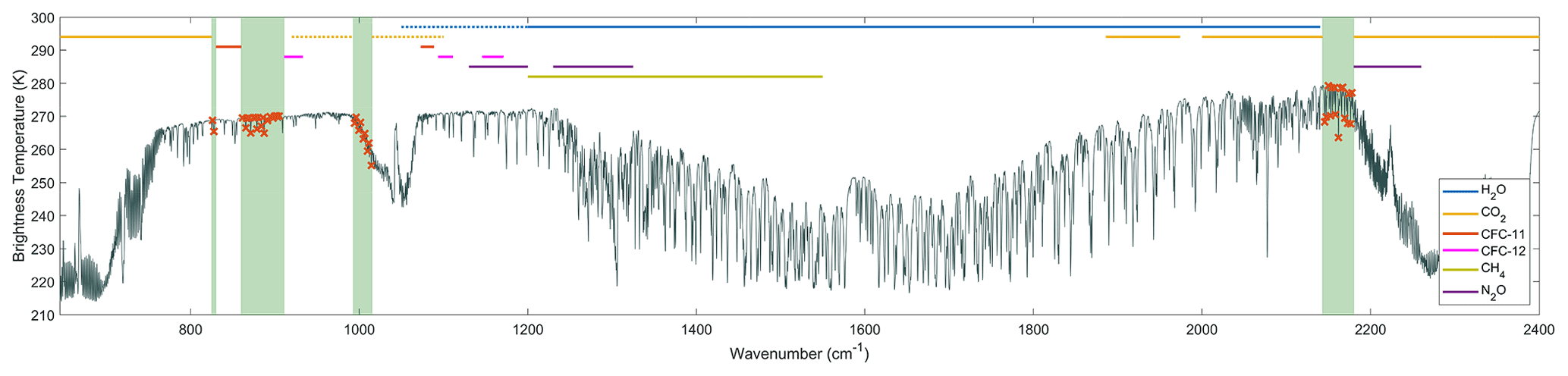
Figure 1Mean IASI spectrum in brightness temperature with the 45 channels selected for the training displayed (red crosses). The shaded green area corresponds to the regions considered for the channel selection. The coloured lines on the top represent the regions of sensitivity to H2O, CO2, CH4, N2O, CFC-11 and CFC-12 excluded.
Table 1List of IASI wavenumbers selected for the training of the cloud detection neural network.
In the remaining spectral regions (see Fig. 1), we selected, from a mean IASI spectrum, channels associated with minimum and maximum brightness temperatures. Indeed, the maxima represent mainly background radiation (coming from either clouds or the surface or both). The minima correspond to channels strongly affected by trace gas absorptions. The difference between the maxima and the minima provides information on cloud opacity. By selecting spectral regions affected by H2O, O3 and CO, respectively, the network is sufficiently robust against local changes in their concentration (e.g. at high latitude the water vapour column is low, but in that case the O3 channels are still available). In practice, the spectral regions were evaluated in groups of 20 channels from which the minimum and the maximum brightness temperature was selected. An exclusion criterion was applied to neighbouring channels (two minima/maxima must be at least three channels apart) to reduce redundancy and ease training of the network (as neighbouring IASI channels are highly correlated). We ended up with 45 channels mainly located in the atmospheric window 1 and 3 and on the low-wavenumber part of the ν3 O3 absorption band. The wavenumbers corresponding to the selected IASI channels are given in Table 1 and are shown in Fig. 1. Note that, as most of the selected channels are located in the atmospheric window regions, the network should be sensitive to clouds at any altitude since the atmosphere at these wavelengths is transparent in the absence of clouds.
To get the training representative of real input data, the training set should be as large and as extensive as possible while remaining reasonable in terms of computational resources required. For this, about 54 000 clear and 54 000 cloud scenes derived from Metop-B observations were taken randomly over 1 year (2020). Since the EUMETSAT IASI-L2 product provides a value of cloud fraction in the IASI pixel, we first converted it into a cloud flag: a scene was considered to be cloud-free only if the cloud fraction was strictly equal to zero. With these and with the corresponding IASI radiance at the 45 selected channels, the NN was trained. The NN consists of a supervised two-layer pattern recognition network (Kothari and Oh, 1993) with one sigmoid hidden layer of 20 neurons and one output layer of one linear neuron. The training algorithm is a Levenberg–Marquardt backpropagation. For the training, the dataset was divided randomly into three parts: (1) the training set (95 %), (2) a validation set (4 %) and a test set (1 %). In addition to the 45 channels, we also included the surface elevation as an input parameter for the NN taken from the “National Geophysical Data Center TerrainBase Global DTM Version 1.0” (ftp://ftp.ngdc.noaa.gov/Solid_Earth/cdroms/TerrainBase_94/, last access: 5 September 2022). In total, we performed 10 different training sessions, and we selected the least affected by dust (see Sect. 4.3). The corresponding MATLAB function containing all the training variables is provided in the Supplement along with an example code showing how to run the network. The training of the network takes, depending on the run, about 100–150 iterations and is completed in about 30 min on a typical personal computer. The performance of the selected training reaches 87.3 % with an equivalent number of misdetections in the clear and cloud group.
The actual retrieval provides a value comprised between 0 and 1. If the average cloud fraction was about 50 % on Earth, the threshold for separating the clear and cloud scenes would be equal to 0.5 as the training was performed with the same number of data in the two groups. However in practice, as mentioned in the introduction, cloud-contaminated scenes dominate, and the optimal threshold (minimizing the differences with the L2) has to be determined. For this, we calculated the mean NN cloud amount for the year 2020 in a 0.25∘ × 0.25∘ grid (calculated as the number of the scenes flagged as cloud over the total number of observations) by considering a set of different thresholds and found the one which minimizes the difference with the L2-derived cloud amount. A separate threshold, of 0.175 (±0.020) and 0.275 (±0.015), respectively, was defined for land and for sea measurements. Those are recommended when the NN cloud product is used for the cloud removal preprocessing phase in satellite data retrieval schemes. However, as we demonstrate in Sect. 4.1, this threshold can be adjusted depending on the application. The uncertainty in the thresholds is estimated by evaluating the change in the threshold for a 1 % increase in the difference between the L2 and the NN.
After application of the network and the threshold to derive the cloud mask, a number of low-temperature observations stood out as being clearly misclassified, having a very low temperature (< 270 K) at mid-latitude (mostly over ocean). While the number of such observations is very low (< 0.2 %), they were important enough to be removed with a postfilter, which was constructed as follows. We built a monthly climatology of the mean and standard deviation of the brightness temperature (BT) calculated for one channel at 821.75 cm−1 on a 1∘ × 1∘ grid from the 2008–2020 data. The channel was carefully selected to avoid the regions of absorption of the main atmospheric absorbers and the wavenumbers strongly affected by the surface type (water, snow, ice, deserts, etc.). Any retrieval initially declared as clear is flagged as cloudy if the BT associated with the measurement is lower than the mean BT minus 3 times its standard deviation for the corresponding month in the 1∘ × 1∘ grid.
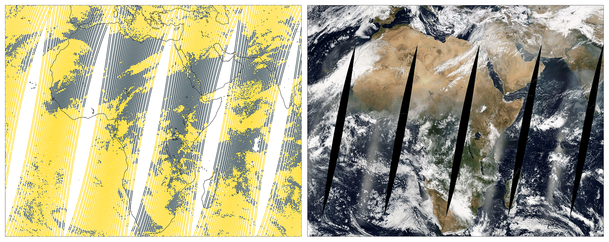
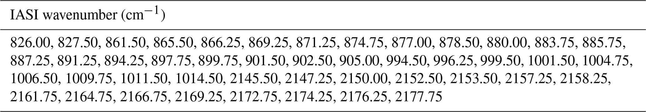
Figure 2Left: example of cloud detection from the IASI neural network algorithm for 1 d of measurements (15 February 2018, morning overpass). Cloud scenes are in yellow, clear-sky scenes in blue. Right: MODIS Terra-corrected reflectance (true colours) imagery for the same day (from NASA Worldview).
An example of retrieved cloud mask on 15 February 2018 for the morning overpasses of IASI over Africa, the Arabian Peninsula and the western part of the Indian Ocean is given in Fig. 2. Yellow points correspond to pixels flagged as cloudy. The MODIS Terra-corrected reflectance imagery for the same day is shown as well. An excellent correspondence is found for the large structures of high opaque clouds and the cloud-free regions (e.g. northern and southern Africa, the Arabian Peninsula). For the regions characterized by sparse cumulus of thin cirrus clouds, the comparison is more difficult because of the different overpass time of the two instruments (10:30/22:30 LT for MODIS Terra and 09:30/21:30 LT for IASI) as the spatial distribution of clouds can evolve very rapidly (due to evaporation, precipitation and transport). A good distinction is also obtained between clouds and dust plumes, as observed on the west coast of Africa north of the Equator. The sensitivity to dust is further assessed in Sect. 4.3.
The entire IASI time series has been processed for Metop-A, Metop-B and Metop-C. The computational time is fast, taking about 2.5 min in CPU time per day processed (on a typical personal computer). For Metop-A before 2017, a reprocessed radiance dataset with the latest version of the L1C has been released by EUMETSAT in 2018 (EUMETSAT, 2018). This allows us to produce a consistent time series of the cloud mask for the 15 years of IASI observations. In this section, we give a short overview of the large-scale cloud regimes and seasonality as captured by the IASI-NN cloud product. The mean cloud amount (%; also referred to synonymously as cloud cover or cloud fraction from here onwards) derived from Metop-A observations separately from the morning and the evening overpasses between 2008 and 2020 in a 0.25∘ × 0.25∘ grid is shown in Fig. 3. It is calculated as the number of observations flagged as cloudy over the total number of observations. The two distributions are very similar, with, on average, differences in the mean cloud amount lower than 2 % for seas and 1 % for land.

Figure 3Mean cloud cover (%) calculated using the IASI neural network cloud detection algorithm between 2008 and 2020 separately for day (a) and night (b) observations in a 0.25∘ × 0.25∘ grid.
The large-scale patterns are very similar to those reported in previous studies (e.g. Wylie and Menzel, 1999; King et al., 2013). In general, clear sky is more common over land than over oceans: globally, about 85 % and 57 % of all observations over seas and land, respectively, are flagged as cloudy. The largest cloud amounts are found at mid-latitudes to high latitudes over oceans, where cold air condenses water vapour into clouds. This is especially the case in the Southern Hemisphere (below about 45∘ S), where the cloud amount exceeds 95 % on average over the year. In the Northern Hemisphere, the North Atlantic and North Pacific (from 40∘ N) exhibit similar values. Close to the Equator, a band of high cloud cover (> 90 %) located at the Intertropical Convergence Zone (ITCZ) corresponding to the region of convergence of the north-eastern and the south-eastern trade winds is also clearly visible. Two other regions characterized by a very high mean cloud cover are located along the coasts of Peru and Chile and in the Atlantic, west of Angola. Conversely, lower cloud amounts of about 50 % to 70 % are observed over the subtropical gyres of the oceans.
Above land, the cloud distribution is more variable, with desert areas characterized by a quasi absence of cloud over the whole year (typically around 20 % for the Sahara and the Arabian Peninsula), while intertropical regions show a cloud cover of about 80 %–85 %. Mid-latitudes and high latitudes in the Northern Hemisphere, for their parts, are typically characterized by a mean cloud fraction of 70 %–75 %. Desert conditions with about 30 % mean cloud cover are also observed in the eastern part of Antarctica, characterized by high altitudes reaching 4 km on the Antarctic Plateau (Listowski et al., 2019). Over high latitudes in the Northern Hemisphere and the Southern Hemisphere globally (between 60 and 90∘ N and S, for land and seas together), we find a mean cloud coverage of about 76 % and 66 %, respectively. While for the Northern Hemisphere, this is in excellent agreement with values reported from the Cloud-Aerosol Lidar and Infrared Pathfinder Satellite Observation (CALIPSO) in Karlsson and Devasthale (2018), the cloud coverage in the Southern Hemisphere might be slightly underestimated by about 10 % (around 76 % from CALIPSO; Karlsson and Devasthale, 2018).
Note the presence of high cloud cover values observed over the high mountain ranges in the different regions of the world (e.g. Himalayas, Ural Mountains, Andes, Rocky Mountains). These are likely exaggerated by false cloud detection due to the climatic conditions in these areas (lower thermal contrast between the surface and the cloud, drier air, etc.) or to the heterogeneity of the topography within the IASI pixel, which makes the distinction between clear and cloudy pixels more difficult. In addition, for the nighttime distribution, patches of slightly higher cloud coverage are observed over deserts, in particular for the Sahara Desert, which probably reflect emissivity features due to inhomogeneity in the land surface properties associated with a lower sensitivity. These patterns over high mountain ranges and deserts are also observed in the distributions derived from other cloud products (see Sect. 4).
Figure 4Seasonal mean daytime cloud cover (%) calculated from the IASI neural network cloud detection algorithm between 2008 and 2020. (a) Winter (December–February), (b) spring (March–May), (c) summer (June–August), (d) autumn (September–November).
When looking at the seasonal average derived over the 2008–2020 period from the daytime measurements (Fig. 4), we find strong variations in agreement with the known seasonal cycles of the clouds around the globe. Close to the Equator, the band of high cloud amount moves progressively in latitude with the ITCZ from its northernmost position around 10∘ N during the boreal summer (Fig. 4c; June–August) to its southernmost position in the boreal winter (Fig. 4a; December–February), in agreement with the observations of King et al. (2013) based on the measurements of the MODIS sounders on board the Terra and Aqua satellites. In the tropical regions (up to about 25∘ N and S), the seasonal variations in Africa south and north of the Equator, in central South America, in India, and in South East Asia are mainly associated with the monsoon with a maximum cloud coverage observed during the boreal summer (winter) for the regions located north (south) of the Equator (Eastman and Warren, 2010; Warren et al., 2015). Northern Australia also experiences cloudy conditions during boreal winter. At mid-latitudes, in the Northern Hemisphere, minimum and maximum cloud amount are observed, as expected, during the summer and the winter months, respectively.
At high latitudes, the Southern Ocean surrounding Antarctica exhibits high mean cloud amount, reaching up to 98 % during the boreal winter and with a minimum of about 88 % during the summer. A more pronounced seasonal cycle is observed around the Weddell Sea and the Ross Sea, with a decrease by an amplitude of about 25 % observed during the boreal summer (Fig. 4c; June–August). Over the Antarctic Plateau, where the mean cloud amount is low, a clear seasonality is also observed. The cloud fraction varies from about 16 % in spring (Fig. 4b; March–May) to about 40 % during autumn (Fig. 4d; September–November). Western Antarctica, for its part, is more cloudy, with a peak of 72 % observed in the boreal winter and a minimum of 52 % in spring. Similar seasonal features and cloud occurrence at high Southern Hemisphere latitudes have also been reported in previous studies relying on CALIPSO observations (Adhikari et al., 2012; Listowski et al., 2019; Karlsson and Devasthale, 2018). In the Northern Hemisphere, the Arctic region shows a strong seasonal cycle as well, more pronounced for the higher latitudes, with a maximum during the boreal summer and a minimum in the winter. These seasonal patterns are in agreement with the observations derived from CALIPSO in Karlsson and Devasthale (2018) and with those reported in Eastman and Warren (2010) based on land, ships and drifting sea ice weather stations.
4.1 Climatological mean
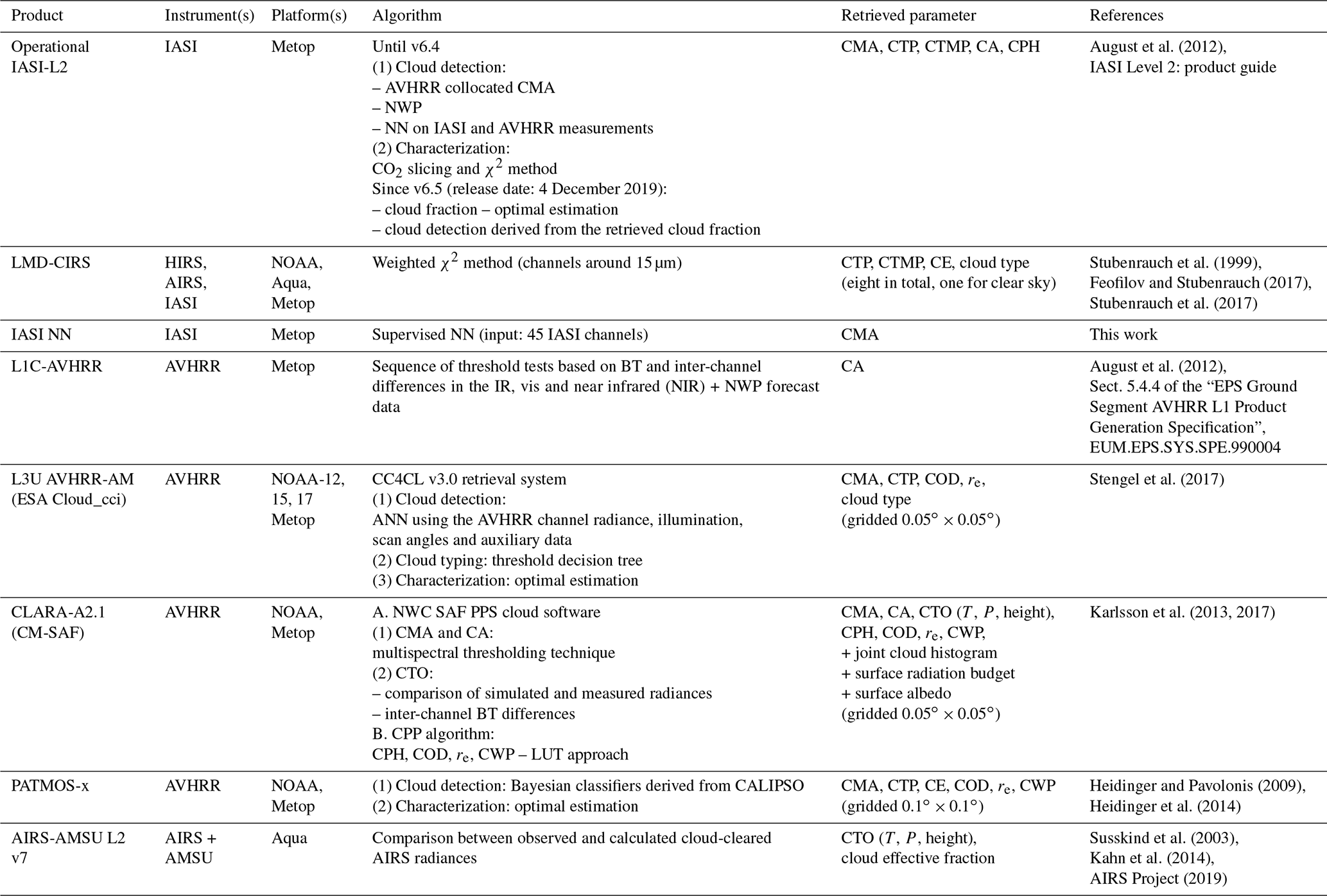
To give a first assessment of the IASI-NN cloud product, we compare here the NN cloud mask with other existing cloud products. We start with average cloud distributions. In total, seven different products are selected for the comparison: the operational IASI-L2, the CIRS-LMD also directly based on the IASI measurements, the L1C-AVHRR and three cloud climate data records (CDRs) built from the measurements of the AVHRR sounder on board the Metop-A satellite. Those are the CLARA-A2.1 produced by the EUMETSAT Climate Monitoring Satellite Application Facility (CM-SAF) (Karlsson et al., 2013, 2017), the Level-3U ESA Cloud_cci (Stengel et al., 2017) and the PATMOS-x (Pathfinder Atmosphere Extended) (Heidinger and Pavolonis, 2009; Heidinger et al., 2014) datasets. We also include a comparison with the Aqua/AIRS L2 (AIRS+AMSU) V7.0 product, despite the different overpass time with IASI (01:30 and 13:30 LT; AIRS Project, 2019). A short description of each cloud product is provided in Table 2. The IASI-L2, the CIRS-LMD and the L1C-AVHRR are also briefly described in the introduction. The three CDRs are based on different retrieval approaches (see Table 2 and references therein). In addition to a cloud mask, they also include a full cloud characterization. The data are provided at a resampled resolution of 0.05∘ × 0.05∘ grid for the CLARA-A2.1 and the ESA Cloud_cci and at 0.1∘ × 0.1∘ for PATMOS-x. The AIRS-AMSU L2 product integrates cloud top level information and the cloud effective fraction.
August et al. (2012)Stubenrauch et al. (1999)Feofilov and Stubenrauch (2017)Stubenrauch et al. (2017)August et al. (2012)Stengel et al. (2017)Karlsson et al. (2013, 2017)Heidinger and Pavolonis (2009)Heidinger et al. (2014)Susskind et al. (2003)Kahn et al. (2014)AIRS Project (2019)Table 2Overview of the cloud characterization and retrieval algorithm for the datasets considered in this study. CMA: cloud mask; CTP: cloud top pressure; CTMP: cloud temperature; CA: cloud amount; CPH: cloud phase; CE: cloud emissivity; COD: cloud optical depth; re: cloud effective radius; CTO: cloud top level; CWP: cloud water path.
The intercomparison is performed over the 2016 data, except for the IASI-L2 product, which is derived from 2020 and the AIRS-AMSU products from 2015 (as AMSU failed in September 2016). For the IASI-L2, this choice was made so that the comparison is performed against the latest version of the L2, which was used for the training of the NN. For the IASI-L2, the L1C-AVHRR and the AIRS-AMSU products, as a cloud mask is not provided, we considered the scenes with a cloud fraction in the field of view (FOV) strictly equal to 0 % to be clear.
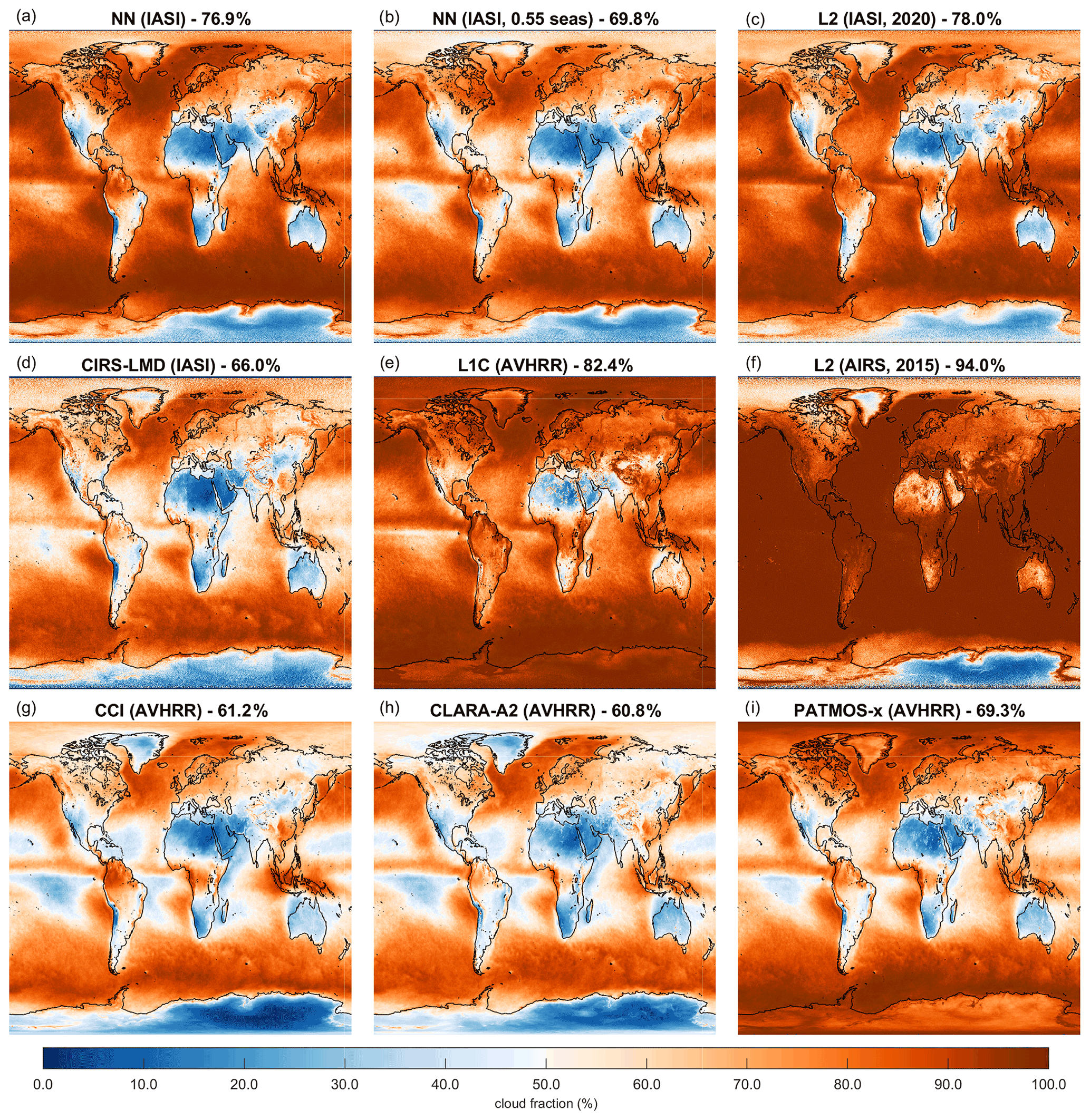
Figure 5One-year-average cloud cover (%) from IASI-, AIRS- and AVHRR-derived cloud products (daytime observations). The year considered for the averaging is 2016, except for the EUMETSAT IASI-L2 product (2020) and the AIRS-L2 product (2015). The global mean cloud cover is provided on top of each panel.
Figure 5 shows the global mean cloud cover (%; daytime measurements only) in a 0.25∘ × 0.25∘ grid for the IASI-NN and the seven cloud products considered for the inter-comparison. We also included the mean cloud amount distribution derived from the NN but with the threshold doubled over seas for the separation between clear-sky and cloud scenes (threshold of 0.55 instead of 0.275). For the three cloud CDRs, their initial resolution was degraded to match the 0.25∘ grid. The cloud fraction is calculated as in Sect. 3 (i.e. the number of observations flagged as cloudy over the total number of observations). As expected, the IASI-NN and the IASI-L2 products (Fig. 5a and c) are very similar, with an identical mean cloud amount of 75.7 % over the whole globe and a correlation coefficient and a mean of the absolute difference between the two distributions of 0.91 and 6.5 %, respectively (5 % when the comparison is done against the IASI-NN distribution for 2020). The same regions of high/low cloud load appear. In general, though, the IASI-NN mean cloud fraction is slightly lower (by about 6 %) than the IASI-L2 in the intertropical regions (between 20∘ N and S), while the opposite is observed for the mid-latitudes and high latitudes north and south of the Equator. This is particularly visible in the Pacific, south of the ITCZ, and in the southern Pacific and southern Atlantic. Over Antarctica, while the cloud fraction is close on average (within 2 %), large regional disparities are observed especially in the eastern part. Along the Antarctic coasts, the cloud distribution derived from the NN is generally higher than the L2 up to about 40 %. Over the Antarctic Plateau, in contrast, the cloud cover is about 5 % lower for the NN (but up to 20 %–25 % locally). Note that the differences between the L2 and the NN do not allow the conclusion of a better performance in the cloud detection for one or the other product as there is no guarantee that the cloud attribution of the L2 is always correct.
The second IASI-derived cloud product, the CIRS-LMD (Fig. 5d), appears to assign clear-sky flags more often than the IASI-NN product, with a mean global cloud fraction (land and sea observation together) of about 66 % (74 % above oceans). Besides that, the same cloud patterns of low and high cloud coverage appear, as reflected by the very good correlation with the NN cloud product (r=0.88). The correspondence in the cloud fraction with the NN becomes much better when the threshold considered for separating the clear sky from the cloud scenes over oceans is doubled (Fig. 5b). With this parametrization, the mean cloud coverage reaches 69 % globally (76 % above oceans only). Note also for both the L2 and the CIRS-LMD product the similar features that were reported for the IASI-NN product (see Sect. 3) in the regions of tall mountain ranges associated with a weaker sensitivity to cloud detection.
The four AVHRR-derived cloud products, for their part, show very different mean cloud amounts. The dataset with the lowest number of scenes flagged as clear is the L1C-AVHRR product (Fig. 5e). Over seas, for tropical and mid-latitude regions (between 50∘ N and S), the cloud amount is close to the one from the IASI-NN product (mean of the absolute difference of about 3 %). At higher latitudes, the difference increases to 9 %. Above land, the differences are much more pronounced and increase with latitude (from about 20 % in the tropics and mid-latitudes to 32 % above 50∘ N and S). This is particularly evident above Antarctica, where a large overestimation of the cloud fraction is observed for the L1C-AVHRR product (mean cloud coverage of 96 %). Large differences that are traceable to specific emissivity features are also present above deserts and over high mountains (e.g. over the Sahara).
The three other AVHRR products (CLARA-A2, CCI and PATMOS-x; Fig. 5g, h, i) show cloud amounts close to those from the CIRS-LMD and the IASI-NN product, with a doubled threshold for the tropical and mid-latitudes regions (around 60 % on average between 50∘ N and S), but with lower fractions observed over the subtropical gyres. The main difference between the three products lies in their sensitivity to cloud detection at high latitudes, especially above 75∘ N and over Antarctica. For the latter, the CLARA-A2 and CCI products are well below the three IASI-derived cloud products (mean cloud coverage of 30 % versus 48 % for IASI-NN) and likely underestimate the cloud amount (Karlsson and Devasthale, 2018). The PATMOS-x product, in contrast, is much more strict in the cloud-free scene attribution, with a mean cloud fraction over Antarctica of 87 %.
Finally, among the eight cloud products analysed here, the one with the lowest number of scenes flagged as clear sky is the AIRS-AMSU L2 (Fig. 5f). Globally, the mean cloud fraction for the year 2015 is 88 %, about 12 % higher than the NN-derived cloud product. Over seas, for the tropical and mid-latitude regions (between 50∘ N and S), the mean value even reaches 99 % (85 % for the NN product). Deserts also show a high cloud coverage compared to the other selected products, with, for example, a mean cloud fraction of 74 % for the Sahara desert against 24 % with the NN product. Only high latitudes present a very similar cloud amount to the NN, with an average cloud coverage of 76 % and 65 % above and below 60∘ N and S, respectively.
4.2 Time series
Figure 6 shows the time series of the global mean fraction of cloud-free scenes for the NN, the EUMETSAT IASI-L2 and the CIRS-LMD cloud masks, derived from Metop-A and Metop-B between 2008 (2013 for Metop-B) and 2020. Currently, the CIRS-LMD data are only available until 2019. Results are presented for land and sea observations together and separate. Both the NN and the CIRS-LMD cloud products show an excellent stability over time, with no visible trends and a very good consistency between the two Metop instruments (absolute difference lower than 1 % on average for the NN). In contrast, the L2 cloud-free time series reveal sharp discontinuities coinciding with version changes. In addition, a clear positive trend is also visible between 2012 and 2020, likely due to the CO2 concentration increase in the atmosphere.

Figure 6Time series of the daily mean fraction of cloud-free scenes for the L2, NN and LMD cloud products (Metop-A and Metop-B) globally for land and sea (a) and for sea (b) and land (c) observations only. The thick lines represent the 30 d moving average.
As expected, the correspondence between the fraction of clear scenes from the NN and from version 6.5 of the IASI-L2 (from December 2019 onward) is excellent, with differences lower than 1 % on average for both land and sea measurements. The fraction of clear scenes above sea and land are about 14 % and 42 % on average, respectively. The CIRS-LMD product, for its part, appears to assign clear sky more often than the IASI-NN product over seas, with about 25 % of all scenes flagged as clear, but shows comparable values (42 %) over land.
When looking at the interannual variations, a clear seasonality appears above land for both the NN and the CIRS-LMD products, with a peak in the clear-sky scenes during the boreal summer. Good agreement in the seasonality is also found with the L2 cloud product from version 6.5 of the L2, but, oddly, the seasonality seems out of phase with the NN (peak occurring during the boreal spring) between 2012 and 2019 (corresponding to version 5.3 to version 6.4 of the L2). The reason for the differences has not been investigated further.
4.3 Dust detection
One important aspect to consider when assessing the quality of a cloud mask is its ability to distinguish clouds from dust plumes. Figure 7 shows examples of days (2 in 2013 and 2 in 2020) when dust plumes are clearly visible above Africa or the eastern Atlantic (right column). Those were selected by analysing the MODIS (Terra)-corrected reflectance (true colours) imagery (https://worldview.earthdata.nasa.gov, last access: 5 September 2022) and a dust index developed by Clarisse et al. (2019) quantifying the strength of the dust signal in the IASI spectrum. For each of them, we plotted the cloud flag derived from the L2 (left) and from the NN (middle column). On top, we also displayed the contour plot of the dust index for two different levels (index of 10 and 20, respectively). For the L2, the IASI pixels seen as cloudy by the L2 but as cloud-free by the NN in the presence of high dust loads (dust index higher than 10) are shown in pink.

Figure 7Cloud detection over north-western Africa from the EUMETSAT IASI-L2 cloud product (left column) and the IASI-NN detection algorithm (middle column) for 4 d (13 February, 24 February, 17 June, 18 June 2020, morning orbits) affected by dust plumes. Yellow and blue circles refer to cloudy and cloud-free scenes, respectively. The right column shows the MODIS (Terra)-corrected reflectance (true colours) imagery for the corresponding days (from NASA Worldview). The contours represent two levels of dust index (10 red and 20 black). The pink circles on the IASI L2 maps show the pixels flagged as cloudy by the L2 and cloud-free by the NN in the presence of high dust loads (cloud index > 10).
As has already been reported in Clarisse et al. (2019), older versions of the operational IASI-L2 cloud product are affected by the presence of dust for the detection of cloud scenes. This can be seen for example on 3 and 7 June 2013 (left panels of the two first rows) with version 5.3.1 of the L2 where the regions of high dust loads (index higher than 10 and 20) are often flagged as cloudy, while no clouds are visible in the MODIS imagery.
In contrast, the NN and version 6.5 of the L2 (v6.5) cloud products seem to fairly differentiate clouds from dust plumes, as observed for example on 8 June 2020 (third line) and also in 2013 for the NN. However, in rare cases, the cloud detection is still affected by the presence of dust, especially over land in the centre of dust plumes. These false cloud detections seem to occur more frequently in the L2 than in the NN. This is for example the case on 7 June 2020 (bottom panels) where the dust index indicates the presence of a high amount of dust over western Mauritania with no cloud visible in the MODIS imagery. In the area, the NN (middle panel) correctly flags the IASI measurements as cloud-free, while the L2 reports the presence of clouds for most of the pixels (pink circles on Fig. 7). Similarly, on 8 June 2020, the bottom part of the area above Niger, where a high amount of dust is observed (dust index > 20), is flagged as cloudy in the L2 and as clear in the NN, while the MODIS map shows the presence of only a few sparse clouds (for the most part detected by the NN). The relatively better performance of the NN compared to the L2 in correctly differentiating dust from clouds may seem counterintuitive as the NN was trained to follow the L2. However, as mentioned in Sect. 2, among the 10 different training sessions performed, we selected the training least affected by dust. The choice was made by analysing the cloud mask retrieved over 17 different dust storms in parallel with the corresponding MODIS true colour imagery and the dust index (Clarisse et al., 2019). In general, on the global scale, the performance of the different training sessions was very close. Note that, apart from the dust, good agreement between the NN and version 6.5 of the L2 is also found for the areas flagged as clear and cloudy and that match with the MODIS true colour maps.
With already more than 15 years of continuous and consistent measurements and at least another 25 years to come with the recent launch of IASI on Metop-C and the future launch of IASI-NG (New Generation, with a spectral sampling of 0.125 cm−1) on the Metop-SG suite of satellites (Crevoisier et al., 2014), the IASI dataset is becoming a fundamental reference climate data record. To be exploited to its full potential, it requires an accurate and unbiased cloud filter. While several cloud products of high quality already exist, they are generally either not homogeneous on the whole IASI time series or not strict enough in the cloud detection for use in satellite data retrieval schemes of geophysical variables. In this paper, we present a new algorithm for the identification of cloud-free scenes in the IASI field of view that is well suited to study trends for IASI-derived trace gases and other climatological variables. The method relies on a neural network (NN) taking a set of 45 IASI radiance channels as input and trained with version 6.5 (v6.5) of the operational IASI Level2 (L2) cloud product as reference. Usually, cloud detection and characterization methods exploit the information derived from CO2-sensitive channels. Here, the channels were selected outside the regions of absorption of CO2, CH4, N2O, CFC-11 and CFC-12 to avoid any long-term biases, as their concentrations evolve over time in the atmosphere. Despite this, we managed to reach excellent performances for the training (87 %), indicating that the information for detecting clouds is also present in other regions of the spectrum. We have shown that the retrieval is both sensitive to the cloud detection and consistent over the entire IASI life span and between the different copies of the IASI instrument on board the suite of Metop satellites. It also differentiates cloud from dust plumes fairly well. While the agreement with the IASI-L2 cloud product was generally very good, with a correspondence of about 87 % overall, differences have been reported over some regions, especially above seas over the subtropical gyres and in the southern Pacific and the southern Atlantic, but without being able to yield a better performance for either product. The agreement with other existing products was generally good in the main cloud regimes, but with sometimes large differences in the mean cloud amount (up to 10 % on average), especially with the three AVHRR cloud climate data records and with the CIRS-LMD IASI cloud retrieval algorithm suite. Given its good performances, the IASI NN cloud product is planned to be implemented in the near future in the Artificial Neural Network for IASI (ANNI) (Franco et al., 2018), the dust (Clarisse et al., 2019) and the spectrally resolved Outgoing Longwave Radiation (Whitburn et al., 2020) IASI retrieval frameworks. Note finally that, in the case of future improvement in the IASI-L2 cloud product, the NN could easily be retrained, and a complete reprocessing of the entire time series of the IASI NN cloud mask could be performed in a short time.
The analysis codes can be made available upon request to the corresponding author. The MATLAB function containing all the training variables is provided in the Supplement along with an example code showing how to run the network.
The daily IASI NN outputs will be made freely available for all users through the IASI-FT website: https://iasi-ft.eu/ (last access: 5 September 2022; Metop-A: https://doi.org/10.21413/IASI-FT_METOPA_CLD_L2_ULB-LATMOS, Whitburn, 2022a; Metop-B: https://doi.org/10.21413/IASI-FT_METOPB_CLD_L2_ULB-LATMOS, Whitburn, 2022b; Metop-C: https://doi.org/10.21413/IASI-FT_METOPC_CLD_L2_ULB-LATMOS, Whitburn, 2022c). For use as cloud removal preprocessing phase in satellite retrieval, we recommend adopting the thresholds mentioned in the paper for land and sea observations, but these can also be adjusted depending on the application.
The supplement related to this article is available online at: https://doi.org/10.5194/amt-15-6653-2022-supplement.
SW and LC came up with the idea and conceptualized the product. SW developed the algorithm and performed the evaluation of the data. MC, TA and TH brought their expertise on the IASI L2 cloud product. PFC and CC contributed to the cloud product through numerous helpful comments and discussions. SW and LC led the writing of the paper, with input from all co-authors.
The contact author has declared that none of the authors has any competing interests.
Publisher’s note: Copernicus Publications remains neutral with regard to jurisdictional claims in published maps and institutional affiliations.
IASI has been developed and built under the responsibility of the Centre National d'Études spatiales (CNES, France). It is flown on board the Metop satellites as part of the EUMETSAT Polar System. The IASI L1C data are received through the EUMETCast near-real-time data distribution service. Simon Whitburn is grateful to the ERC for funding his research work. Lieven Clarisse is a research associate (Chercheur Qualifié) supported by the Belgian F.R.S.-FNRS. Cathy Clerbaux is grateful to CNES for scientific collaboration and financial support. We acknowledge the use of imagery from the NASA Worldview application (https://worldview.earthdata.nasa.gov), part of the NASA Earth Observing System Data and Information System (EOSDIS).
This research has been supported by the European Research Council (ERC) under the European Union’s Horizon 2020 research and innovation programme (grant agreement no. 742909, IASI-FT advanced ERC grant) and the PRODEX arrangement HIRS (Belspo-ESA).
This paper was edited by Linlu Mei and reviewed by Artem Feofilov and one anonymous referee.
Adhikari, L., Wang, Z., and Deng, M.: Seasonal variations of Antarctic clouds observed by CloudSat and CALIPSO satellites, J. Geophys. Res.-Atmos., 117, D04202, https://doi.org/10.1029/2011jd016719, 2012. a
AIRS project: Aqua/AIRS L2 Support Retrieval (AIRS+AMSU) V7.0, Greenbelt, MD, USA, Goddard Earth Sciences Data and Information Services Center (GES DISC), https://doi.org/10.5067/TZ6I8E3ODIQB, 2019. a, b
August, T., Klaes, D., Schlüssel, P., Hultberg, T., Crapeau, M., Arriaga, A., O'Carroll, A., Coppens, D., Munro, R., and Calbet, X.: IASI on Metop-A: Operational Level 2 retrievals after five years in orbit, J. Quant. Spectrosc. Ra., 113, 1340–1371, https://doi.org/10.1016/j.jqsrt.2012.02.028, 2012. a, b, c, d, e, f
Bouillon, M., Safieddine, S., Hadji-Lazaro, J., Whitburn, S., Clarisse, L., Doutriaux-Boucher, M., Coppens, D., August, T., Jacquette, E., and Clerbaux, C.: Ten-Year Assessment of IASI Radiance and Temperature, Remote Sens., 12, 2393, https://doi.org/10.3390/rs12152393, 2020. a, b
Capelle, V., Chédin, A., Pondrom, M., Crevoisier, C., Armante, R., Crepeau, L., and Scott, N. A.: Infrared dust aerosol optical depth retrieved daily from IASI and comparison with AERONET over the period 2007–2016, Remote Sens. Environ., 206, 15–32, https://doi.org/10.1016/j.rse.2017.12.008, 2018. a
Chen, X. and Huang, X.: Deriving clear-sky longwave spectral flux from spaceborne hyperspectral radiance measurements: a case study with AIRS observations, Atmos. Meas. Tech., 9, 6013–6023, https://doi.org/10.5194/amt-9-6013-2016, 2016. a
Clarisse, L., Clerbaux, C., Franco, B., Hadji-Lazaro, J., Whitburn, S., Kopp, A. K., Hurtmans, D., and Coheur, P.-F.: A Decadal Data Set of Global Atmospheric Dust Retrieved From IASI Satellite Measurements, J. Geophys. Res.-Atmos., 124, 1618–1647, https://doi.org/10.1029/2018jd029701, 2019. a, b, c, d, e, f
Clerbaux, C., Boynard, A., Clarisse, L., George, M., Hadji-Lazaro, J., Herbin, H., Hurtmans, D., Pommier, M., Razavi, A., Turquety, S., Wespes, C., and Coheur, P.-F.: Monitoring of atmospheric composition using the thermal infrared IASI/MetOp sounder, Atmos. Chem. Phys., 9, 6041–6054, https://doi.org/10.5194/acp-9-6041-2009, 2009. a
Crevoisier, C., Clerbaux, C., Guidard, V., Phulpin, T., Armante, R., Barret, B., Camy-Peyret, C., Chaboureau, J.-P., Coheur, P.-F., Crépeau, L., Dufour, G., Labonnote, L., Lavanant, L., Hadji-Lazaro, J., Herbin, H., Jacquinet-Husson, N., Payan, S., Péquignot, E., Pierangelo, C., Sellitto, P., and Stubenrauch, C.: Towards IASI-New Generation (IASI-NG): impact of improved spectral resolution and radiometric noise on the retrieval of thermodynamic, chemistry and climate variables, Atmos. Meas. Tech., 7, 4367–4385, https://doi.org/10.5194/amt-7-4367-2014, 2014. a, b
De Longueville, H., Clarisse, L., Whitburn, S., Franco, B., Bauduin, S., Clerbaux, C., Camy-Peyret, C., and Coheur, P.-F.: Identification of Short and Long-Lived Atmospheric Trace Gases From IASI Space Observations, Geophysical Res. Lett., 48, e2020GL091742, https://doi.org/10.1029/2020gl091742, 2021. a
DeSouza-Machado, S. G., Strow, L. L., Imbiriba, B., McCann, K., Hoff, R. M., Hannon, S. E., Martins, J. V., Tanré, D., Deuzé, J. L., Ducos, F., and Torres, O.: Infrared retrievals of dust using AIRS: Comparisons of optical depths and heights derived for a North African dust storm to other collocated EOS A-Train and surface observations, J. Geophys. Res., 115, D15201, https://doi.org/10.1029/2009jd012842, 2010. a
Eastman, R. and Warren, S. G.: Interannual Variations of Arctic Cloud Types in Relation to Sea Ice, J. Climate, 23, 4216–4232, https://doi.org/10.1175/2010jcli3492.1, 2010. a, b
EUMETSAT: IASI Level 1C Climate Data Record Release 1 – Metop-A, European Organisation for the Exploitation of Meteorological Satellites, https://doi.org/10.15770/EUM_SEC_CLM_0014, 2018. a
Farouk, I., Fourrié, N., and Guidard, V.: Homogeneity criteria from AVHRR information within IASI pixels in a numerical weather prediction context, Atmos. Meas. Tech., 12, 3001–3017, https://doi.org/10.5194/amt-12-3001-2019, 2019. a
Feofilov, A. G. and Stubenrauch, C. J.: LMD cloud retrieval using IR Sounders. Algorithm Theoretical Basis Document (ATBD) for CIRS-LMD software package (v2), IASI AERIS repository [data set], https://doi.org/10.13140/RG.2.2.15812.63361, 2017. a, b, c, d, e, f
Franco, B., Clarisse, L., Stavrakou, T., Müller, J.-F., Van Damme, M., Whitburn, S., Hadji-Lazaro, J., Hurtmans, D., Taraborrelli, D., Clerbaux, C., and Coheur, P.-F.: A General Framework for Global Retrievals of Trace Gases From IASI: Application to Methanol, Formic Acid, and PAN, J. Geophys. Res.-Atmos., 123, 13963–13984, https://doi.org/10.1029/2018jd029633, 2018. a
Guidard, V., Fourrié, N., Brousseau, P., and Rabier, F.: Impact of IASI assimilation at global and convective scales and challenges for the assimilation of cloudy scenes, Q. J. Roy. Meteor. Soc., 137, 1975–1987, https://doi.org/10.1002/qj.928, 2011. a, b
Heidinger, A. K. and Pavolonis, M. J.: Gazing at Cirrus Clouds for 25 Years through a Split Window. Part I: Methodology, J. Appl. Meteorol. Clim., 48, 1100–1116, https://doi.org/10.1175/2008jamc1882.1, 2009. a, b
Heidinger, A. K., Foster, M. J., Walther, A., and Zhao, X. T.: The Pathfinder Atmospheres–Extended AVHRR Climate Dataset, B. Am. Meteorol. Soc., 95, 909–922, https://doi.org/10.1175/bams-d-12-00246.1, 2014. a, b
Hilton, F., Armante, R., August, T., Barnet, C., Bouchard, A., Camy-Peyret, C., Capelle, V., Clarisse, L., Clerbaux, C., Coheur, P.-F., Collard, A., Crevoisier, C., Dufour, G., Edwards, D., Faijan, F., Fourrié, N., Gambacorta, A., Goldberg, M., Guidard, V., Hurtmans, D., Illingworth, S., Jacquinet-Husson, N., Kerzenmacher, T., Klaes, D., Lavanant, L., Masiello, G., Matricardi, M., McNally, A., Newman, S., Pavelin, E., Payan, S., Péquignot, E., Peyridieu, S., Phulpin, T., Remedios, J., Schlüssel, P., Serio, C., Strow, L., Stubenrauch, C., Taylor, J., Tobin, D., Wolf, W., and Zhou, D.: Hyperspectral Earth Observation from IASI: Five Years of Accomplishments, B. Am. Meteorol. Soc., 93, 347–370, https://doi.org/10.1175/BAMS-D-11-00027.1, 2012. a
IASI Level 2: Product Guide, EUMETSAT, Darmstadt, Germany, https://www.eumetsat.int/media/45982 (last access: 2 September 2022), 2017. a, b
Kahn, B. H., Irion, F. W., Dang, V. T., Manning, E. M., Nasiri, S. L., Naud, C. M., Blaisdell, J. M., Schreier, M. M., Yue, Q., Bowman, K. W., Fetzer, E. J., Hulley, G. C., Liou, K. N., Lubin, D., Ou, S. C., Susskind, J., Takano, Y., Tian, B., and Worden, J. R.: The Atmospheric Infrared Sounder version 6 cloud products, Atmos. Chem. Phys., 14, 399–426, https://doi.org/10.5194/acp-14-399-2014, 2014. a
Karlsson, K.-G. and Devasthale, A.: Inter-Comparison and Evaluation of the Four Longest Satellite-Derived Cloud Climate Data Records: CLARA-A2, ESA Cloud CCI V3, ISCCP-HGM, and PATMOS-x, Remote Sens., 10, 1567, https://doi.org/10.3390/rs10101567, 2018. a, b, c, d, e
Karlsson, K.-G., Riihelä, A., Müller, R., Meirink, J. F., Sedlar, J., Stengel, M., Lockhoff, M., Trentmann, J., Kaspar, F., Hollmann, R., and Wolters, E.: CLARA-A1: a cloud, albedo, and radiation dataset from 28 yr of global AVHRR data, Atmos. Chem. Phys., 13, 5351–5367, https://doi.org/10.5194/acp-13-5351-2013, 2013. a, b, c
Karlsson, K.-G., Anttila, K., Trentmann, J., Stengel, M., Fokke Meirink, J., Devasthale, A., Hanschmann, T., Kothe, S., Jääskeläinen, E., Sedlar, J., Benas, N., van Zadelhoff, G.-J., Schlundt, C., Stein, D., Finkensieper, S., Håkansson, N., and Hollmann, R.: CLARA-A2: the second edition of the CM SAF cloud and radiation data record from 34 years of global AVHRR data, Atmos. Chem. Phys., 17, 5809–5828, https://doi.org/10.5194/acp-17-5809-2017, 2017. a, b, c
Kaspar, F., Hollmann, R., Lockhoff, M., Karlsson, K.-G., Dybbroe, A., Fuchs, P., Selbach, N., Stein, D., and Schulz, J.: Operational generation of AVHRR-based cloud products for Europe and the Arctic at EUMETSAT's Satellite Application Facility on Climate Monitoring (CM-SAF), Adv. Sci. Res., 3, 45–51, https://doi.org/10.5194/asr-3-45-2009, 2009. a
King, M. D., Platnick, S., Menzel, W. P., Ackerman, S. A., and Hubanks, P. A.: Spatial and Temporal Distribution of Clouds Observed by MODIS Onboard the Terra and Aqua Satellites, IEEE T. Geosci. Remote, 51, 3826–3852, https://doi.org/10.1109/tgrs.2012.2227333, 2013. a, b
Kothari, S. C. and Oh, H.: Neural Networks for Pattern Recognition, in: Advances in Computers, Elsevier, 119–166, https://doi.org/10.1016/s0065-2458(08)60404-0, 1993. a
Lavanant, L., Fourrié, N., Gambacorta, A., Grieco, G., Heilliette, S., Hilton, F. I., Kim, M.-J., McNally, A. P., Nishihata, H., Pavelin, E. G., and Rabier, F.: Comparison of cloud products within IASI footprints for the assimilation of cloudy radiances, Q. J. Roy. Meteor. Soc., 137, 1988–2003, https://doi.org/10.1002/qj.917, 2011. a
Listowski, C., Delanoë, J., Kirchgaessner, A., Lachlan-Cope, T., and King, J.: Antarctic clouds, supercooled liquid water and mixed phase, investigated with DARDAR: geographical and seasonal variations, Atmos. Chem. Phys., 19, 6771–6808, https://doi.org/10.5194/acp-19-6771-2019, 2019. a, b
Loeb, N. G., Manalo-Smith, N., Kato, S., Miller, W. F., Gupta, S. K., Minnis, P., and Wielicki, B. A.: Angular Distribution Models for Top-of-Atmosphere Radiative Flux Estimation from the Clouds and the Earth's Radiant Energy System Instrument on the Tropical Rainfall Measuring Mission Satellite. Part I: Methodology, J. Appl. Meteorol., 42, 240–265, https://doi.org/10.1175/1520-0450(2003)042<0240:admfto>2.0.co;2, 2003. a
Rossow, W. B. and Schiffer, R. A.: Advances in Understanding Clouds from ISCCP, B. Am. Meteorol. Soc., 80, 2261–2287, https://doi.org/10.1175/1520-0477(1999)080<2261:aiucfi>2.0.co;2, 1999. a
Safieddine, S., Parracho, A. C., George, M., Aires, F., Pellet, V., Clarisse, L., Whitburn, S., Lezeaux, O., Thépaut, J.-N., Hersbach, H., Radnoti, G., Goettsche, F., Martin, M., Doutriaux-Boucher, M., Coppens, D., August, T., Zhou, D. K., and Clerbaux, C.: Artificial Neural Networks to Retrieve Land and Sea Skin Temperature from IASI, Remote Sens., 12, 2777, https://doi.org/10.3390/rs12172777, 2020. a
Satoh, M., Noda, A. T., Seiki, T., Chen, Y.-W., Kodama, C., Yamada, Y., Kuba, N., and Sato, Y.: Toward reduction of the uncertainties in climate sensitivity due to cloud processes using a global non-hydrostatic atmospheric model, Progress in Earth and Planetary Science, 5, 67, https://doi.org/10.1186/s40645-018-0226-1, 2018. a
Saunders, R. W., Blackmore, T. A., Candy, B., Francis, P. N., and Hewison, T. J.: Ten Years of Satellite Infrared Radiance Monitoring With the Met Office NWP Model, IEEE T. Geosci. Remote, 59, 4561–4569, https://doi.org/10.1109/tgrs.2020.3015257, 2021. a
Schiffer, R. A. and Rossow, W. B.: The International Satellite Cloud Climatology Project (ISCCP): The First Project of the World Climate Research Programme, B. Am. Meteorol. Soc., 64, 779–784, https://doi.org/10.1175/1520-0477-64.7.779, 1983. a
Schneider, T., Teixeira, J., Bretherton, C. S., Brient, F., Pressel, K. G., Schär, C., and Siebesma, A. P.: Climate goals and computing the future of clouds, Nat. Clim. Change, 7, 3–5, https://doi.org/10.1038/nclimate3190, 2017. a
Stengel, M., Stapelberg, S., Sus, O., Schlundt, C., Poulsen, C., Thomas, G., Christensen, M., Carbajal Henken, C., Preusker, R., Fischer, J., Devasthale, A., Willén, U., Karlsson, K.-G., McGarragh, G. R., Proud, S., Povey, A. C., Grainger, R. G., Meirink, J. F., Feofilov, A., Bennartz, R., Bojanowski, J. S., and Hollmann, R.: Cloud property datasets retrieved from AVHRR, MODIS, AATSR and MERIS in the framework of the Cloud_cci project, Earth Syst. Sci. Data, 9, 881–904, https://doi.org/10.5194/essd-9-881-2017, 2017. a, b, c
Stubenrauch, C. J., Rossow, W. B., Chéruy, F., Chédin, A., and Scott, N. A.: Clouds as Seen by Satellite Sounders (3I) and Imagers (ISCCP). Part I: Evaluation of Cloud Parameters, J. Climate, 12, 2189–2213, https://doi.org/10.1175/1520-0442(1999)012<2189:casbss>2.0.co;2, 1999. a, b
Stubenrauch, C. J., Feofilov, A. G., Protopapadaki, S. E., and Armante, R.: Cloud climatologies from the infrared sounders AIRS and IASI: strengths and applications, Atmos. Chem. Phys., 17, 13625–13644, https://doi.org/10.5194/acp-17-13625-2017, 2017. a, b, c, d, e, f, g
Susskind, J., Barnet, C. D., and Blaisdell, J. M.: Retrieval of atmospheric and surface parameters from AIRS/AMSU/HSB data in the presence of clouds, IEEE T. Geosci. Remote, 41, 390–409, https://doi.org/10.1109/tgrs.2002.808236, 2003. a
Van Damme, M., Whitburn, S., Clarisse, L., Clerbaux, C., Hurtmans, D., and Coheur, P.-F.: Version 2 of the IASI NH3 neural network retrieval algorithm: near-real-time and reanalysed datasets, Atmos. Meas. Tech., 10, 4905–4914, https://doi.org/10.5194/amt-10-4905-2017, 2017. a
Warner, J., Carminati, F., Wei, Z., Lahoz, W., and Attié, J.-L.: Tropospheric carbon monoxide variability from AIRS under clear and cloudy conditions, Atmos. Chem. Phys., 13, 12469–12479, https://doi.org/10.5194/acp-13-12469-2013, 2013. a
Warren, S., Eastman, R., and Hahn, C. J.: Clouds and Fog Climatology, in: Encyclopedia of Atmospheric Sciences, Elsevie, 161–169 r, https://doi.org/10.1016/b978-0-12-382225-3.00113-4, 2015. a
Whitburn, S.: A CO2-independant cloud mask from IASI radiances for climate applications (from IASI/Metop-A), ULB/LATMOS [data set], https://doi.org/10.21413/IASI-FT_METOPA_CLD_L2_ULB-LATMOS, 2022a. a
Whitburn, S.: A CO2-independant cloud mask from IASI radiances for climate applications (from IASI/Metop-B), ULB/LATMOS [data set], https://doi.org/10.21413/IASI-FT_METOPB_CLD_L2_ULB-LATMOS, 2022b. a
Whitburn, S.: A CO2-independant cloud mask from IASI radiances for climate applications (from IASI/Metop-C), ULB/LATMOS [data set], https://doi.org/10.21413/IASI-FT_METOPC_CLD_L2_ULB-LATMOS, 2022c. a
Whitburn, S., Clarisse, L., Bauduin, S., George, M., Hurtmans, D., Safieddine, S., Coheur, P. F., and Clerbaux, C.: Spectrally resolved fluxes from IASI data: Retrieval algorithm for clear-sky measurements, J. Climate, 33, 6971–6988, https://doi.org/10.1175/jcli-d-19-0523.1, 2020. a, b
Whitburn, S., Clarisse, L., Bouillon, M., Safieddine, S., George, M., Dewitte, S., Longueville, H. D., Coheur, P.-F., and Clerbaux, C.: Trends in spectrally resolved outgoing longwave radiation from 10 years of satellite measurements, npj Climate and Atmospheric Science, 4, 48, https://doi.org/10.1038/s41612-021-00205-7, 2021. a
Winker, D. M.: The CALIPSO Mission and Initial Observations of Aerosols and Clouds from CALIOP, in: Fourier Transform Spectroscopy/Hyperspectral Imaging and Sounding of the Environment, OSA, Santa Fe, New Mexico, USA, 11–15 February 2007, https://doi.org/10.1364/hise.2007.htud1, 2007. a
Wylie, D. P. and Menzel, W. P.: Eight Years of High Cloud Statistics Using HIRS, J. Climate, 12, 170–184, https://doi.org/10.1175/1520-0442(1999)012<0170:eyohcs>2.0.co;2, 1999. a
Zelinka, M. D., Randall, D. A., Webb, M. J., and Klein, S. A.: Clearing clouds of uncertainty, Nat. Clim. Change, 7, 674–678, https://doi.org/10.1038/nclimate3402, 2017. a
- Abstract
- Introduction
- The neural network: set-up, training, retrieval and postfiltering
- Average distributions
- Assessment and intercomparison
- Conclusions
- Code availability
- Data availability
- Author contributions
- Competing interests
- Disclaimer
- Acknowledgements
- Financial support
- Review statement
- References
- Supplement