TUNER-compliant error estimation for MIPAS: methodology

This paper describes the error estimation for temperature and trace gas mixing ratios retrieved from the Michelson Interferometer for Passive Atmospheric Sounding (MIPAS) limb emission spectra. The following error sources are taken into account: measurement noise, propagated temperature and pointing noise, uncertainties in the abundances of spectrally interfering species, instrument line shape errors, and spectroscopic data uncertainties in terms of line intensities and broadening coefficients. Furthermore, both the direct impact of volatile and persistent gain calibration uncertainties, offset calibration, and spectral calibration uncertainties, as well as their impact through propagated calibration-related temperature and pointing uncertainties, are considered. An error source specific to the MIPAS upper atmospheric observation mode is the propagation of the smoothing error crosstalk of the combined NO and temperature retrieval. Whenever non-local thermodynamic equilibrium modelling is used in the retrieval, related kinetic constants and mixing ratios of species involved in the modelling of populations of excitational states also contribute to the error budget. Both generalized Gaussian error propagation and perturbation studies are used to estimate the error components. Error correlations are taken into account. Estimated uncertainties are provided for a multitude of atmospheric conditions. Some error sources were found to contribute both to the random and the systematic component of the total estimated error. The sequential nature of the MIPAS retrievals gives rise to entangled errors. These are caused by error sources that affect the uncertainty in the final data product via multiple pathways, i.e., on the one hand, directly, and, on the other hand, via errors caused in a preceding retrieval step. These errors tend to partly compensate for each other. The hard-to-quantify effect of the horizontally non-homogeneous atmosphere and unknown error correlations of spectroscopic data are considered to be the major limitations of the MIPAS error estimation.

1 Introduction

The availability of reliable and traceable uncertainty estimates is a precondition for quantitative scientific work with remotely sensed atmospheric temperature and composition data. In order to serve this purpose, we present the scheme according to which error estimation is performed for the composition data retrieved from version 8 limb emission spectra recorded with the Michelson Interferometer for Passive Atmospheric Sounding (MIPAS; Fischer et al., 2008) on Envisat. This error estimation procedure refers to retrievals performed with the data processor developed and operated by the Institute of Meteorology and Climate Research (IMK) in cooperation with the Instituto de Astrofísica de Andalucía (IAA). A general description of the processor is found in von Clarmann et al. (2003). The application to non-local thermodynamic equilibrium conditions is documented in Funke et al. (2001, 2012). The processing of MIPAS spectra measured at reduced spectral resolution after an instrument failure in 2004 is described by von Clarmann et al. (2009). Kiefer et al. (2021) describe the first application to MIPAS version 8 spectra.

The error estimation of the preceding MIPAS retrievals took into account all known major uncertainties but left room for improvement with respect to error correlation issues. It is the purpose of this paper to present a scheme that explores all available knowledge on the ingoing uncertainties, and, in particular, error correlations. We try to comply as much as possible with the recommendations on unified error reporting as specified by the Stratosphere–troposphere Processes And their Role in Climate (SPARC) activity Towards Unified Error Reporting (TUNER), as presented in von Clarmann et al. (2020).

MIPAS temperature and tangent altitude pointing errors are already described in Kiefer et al. (2021). This paper provides an update of their temperature error estimation scheme and aims at having a general scheme for MIPAS trace gas retrieval error estimation. First, the notation used is clarified (Sect. 2), and the error propagation schemes used for MIPAS are introduced (Sect. 3). After the clarification of terminological issues (Sect. 4), we select the scenarios for which uncertainty estimates are carried out and how any arbitrary measurement is linked to these representative uncertainty estimates (Sect. 5). Then, for all relevant error sources, the respective error propagation scheme is discussed for the MIPAS temperature and tangent altitude pointing retrieval (Sect. 6) and retrieved volume mixing ratios (VMRs) of trace constituents (Sect. 7). The MIPAS ozone retrieval serves as an example to illustrate the application of the error estimation scheme (Sect. 9). In Sect. 10, we describe how representative error estimates are built from the sample of analysed observations. The aggregation of component errors to total, random, and systematic error budgets is described in Sect. 11. Technical issues needed to make theory work are presented in Sect. 12. Finally, in Sect. 13, we summarize to which degree we succeeded in providing a robust error estimate and critically identify issues that could not be solved in a satisfactory manner.

2 Definitions and notation

In agreement with the general concept by Rodgers (2000) and the notation suggested by von Clarmann et al. (2020), we use the following retrieval equation for MIPAS:

$$\begin{array}{}\text{(1)}& \begin{array}{ll}{\widehat{\mathit{x}}}_{i+\mathrm{1}}& ={\widehat{\mathit{x}}}_i+{\left({\mathbf{K}}^T{\mathbf{S}}_{y,\text{noise}}^{-\mathrm{1}}\mathbf{K}+\mathbf{R}\right)}^{-\mathrm{1}}\\ & \left({\mathbf{K}}^T{\mathbf{S}}_{y,\text{noise}}^{-\mathrm{1}}\left(\mathit{y}-\mathit{F}({\widehat{\mathit{x}}}_i;\mathit{b})\right)-\mathbf{R}({\widehat{\mathit{x}}}_i-{\mathit{x}}_{\text{a}})\right),\end{array}\end{array}$$

where x is the vector of the target variable, $\widehat{\mathit{x}}$ is its estimate, i denotes the number of iteration, K is the Jacobian with elements $\partial y_m/\partial x_n$, ^T denotes transposed matrices, S_y,noise is the measurement noise covariance matrix, R is the regularization matrix, F is the radiative transfer function. In our case, it is the Karlsruhe Optimized and Precise Radiative transfer Algorithm (KOPRA) radiative transfer model (Stiller, 2000). b is a vector representing all other input parameters except the target variables of the retrieval, x_a is the vector representing the a priori knowledge on the target variables, and x is the vector representing the measurements from the limb scan under investigation, including all tangent altitudes and all spectral points used.

If an inverse a priori covariance matrix, ${\mathbf{S}}_{\mathrm{a}}^{-\mathrm{1}}$, is chosen for the regularization matrix, R, then this formalism represents the optimal estimation or maximum a posteriori retrieval scheme endorsed by Rodgers (2000). However, other choices are possible (see, e.g., Steck and von Clarmann, 2001).

The inverse problem is decomposed species-wise. That is to say, after the retrieval of the temperature and pointing information (Kiefer et al., 2021), ozone concentrations are retrieved in microwindows, where the ozone signal is prominent and where interferences by other gases are low. As a next step, H₂O concentrations are retrieved in spectral microwindows adequate for the H₂O retrieval. In this manner, the retrieval proceeds through the list of species, according to their dominance in the spectrum, where the concentrations of the pre-retrieved species are usually used for the retrieval of the gas currently under analysis. The latter we call target species.

Within linear theory, we have the averaging kernel matrix,

$$\begin{array}{}\text{(2)}& {\displaystyle \frac{\partial \widehat{\mathit{x}}}{\partial \mathit{x}}}=\mathbf{A}={\left({\mathbf{K}}^T{\mathbf{S}}_{y,\text{noise}}^{-\mathrm{1}}\mathbf{K}+\mathbf{R}\right)}^{-\mathrm{1}}{\mathbf{K}}^T{\mathbf{S}}_{y,\text{noise}}^{-\mathrm{1}}\mathbf{K},\end{array}$$

and the gain matrix,

$$\begin{array}{}\text{(3)}& {\displaystyle \frac{\partial \widehat{\mathit{x}}}{\partial \mathit{y}}}=\mathbf{G}={\left({\mathbf{K}}^T{\mathbf{S}}_{y,\text{noise}}^{-\mathrm{1}}\mathbf{K}+\mathbf{R}\right)}^{-\mathrm{1}}{\mathbf{K}}^T{\mathbf{S}}_{y,\text{noise}}^{-\mathrm{1}}.\end{array}$$

For estimated errors, covariances, and so on, we use the TUNER notation. The first subscript denotes the quantity to which the estimated error refers, and the second subscript denotes the source of the error. For example, S_O3; noise is the covariance matrix characterizing the ozone error component due to measurement noise. Beyond this, we use σ_q for standard deviations of a generic variable q and Δq for perturbations with a sign, where

$$\begin{array}{}\text{(4)}& \left|{\mathrm{\Delta }}_{b}q\right|={\mathit{\sigma }}_{q;b},\end{array}$$

and where b denotes the error source.

3 Error propagation

MIPAS retrievals depend on measured spectra and auxiliary information which both are uncertain. Depending on the uncertainty information available, different schemes to estimate error propagation are in use. All error estimations used for MIPAS rely on linear error estimation.

Gaussian error propagation is applied to measurement errors for which the complete covariance information in the measurement domain is available, as follows:

$$\begin{array}{}\text{(5)}& {\mathbf{S}}_{x;\text{meas}}={\mathbf{GS}}_{y;\text{meas}}{\mathbf{G}}^T,\end{array}$$

where S_x;meas is the covariance matrix representing the error in the retrieved variables caused by the measurement error S_y;meas. In this formulation, S_y;meas is a placeholder and will be replaced by the specific type of measurement error under assessment, e.g. noise and calibration errors.

The gain matrix G does not only include the sensitivities of the target gas with respect to the measurement but also the sensitivities of all variables which are fitted along with the target gas in the same inversion, e.g. background continua or further gases that are simultaneously fitted. These gain matrices are available from the retrieval and do not have to be newly evaluated. The resulting covariance matrix S_x;meas includes also entries for all joint fit variables that are fitted along with the target variables for various reasons.

For parameter errors whose covariance information in the altitude domain is available, the parameter uncertainties can be linearly mapped into the measurement domain and then propagated into the target variable space as follows:

$$\begin{array}{}\text{(6)}& {\mathbf{S}}_{x;b}={\mathbf{GK}}_b{\mathbf{S}}_{b;\text{meas}}{\mathbf{K}}_b^T{\mathbf{G}}^T,\end{array}$$

where S_x;b is the covariance matrix representing the error in the retrieved variables caused by the parameter error S_b, and K_b is the Jacobian, representing the sensitivities of the radiance in the analysis windows of the target gas x with respect to changes in the parameter profile b. If b is obtained in a preceding retrieval of the sequential retrieval chain, then it has to be noted that K_b is not the same as the Jacobian used in the preceding retrieval of b because it refers to the spectral radiances in the microwindows used for the retrieval of the target gas x, as opposed to those used in preceding retrieval of b. Thus, it is not available as a byproduct of the temperature and pointing retrieval but needs to be calculated with a dedicated call of the forward model.

Sensitivity studies based on the difference between perturbed spectra (F_perturbed) and nominal spectra (F_nominal) are an alternative when the methods presented above are not applicable or inadequate. Within linear error estimation, the estimated error is proportional to the spectral difference caused by the erroneous quantity. The effect of a 1σ uncertainty in any parameter b_k affecting the signal y can be estimated by perturbing b_k in the input of a run of the forward model F(x,b) by the respective Δb. The response of the retrieval to this perturbation is then estimated as follows:

$$\begin{array}{}\text{(7)}& {\mathrm{\Delta }}_{b_k}\mathit{x}=-\mathbf{G}\cdot ({\mathit{F}}_{\text{perturbed}}-{\mathit{F}}_{\text{nominal}}).\end{array}$$

Here F_nominal are the radiances simulated with the input data and results of the retrieval of x, while F_perturbed are the spectral radiances obtained after perturbation of the parameter(s) under assessment by 1σ. Many applications of Eq. (7) are sign sensitive. That is to say, contrary to the application of variances, the signs of the elements of ${\mathrm{\Delta }}_{{\text{b}}_k}\mathit{x}$ have to be considered. The negative sign on the right-hand side of Eq. (7) is due to the fact that perturbations are applied to the $\mathit{F}(\widehat{{\mathit{x}}_i};\mathit{b})$ term in Eq. (1), which appears with a negative sign there. In order to avoid confusion with respect to the signs, we consistently use the convention that instrumental uncertainties such as gain calibration or instrument line shape uncertainties are understood as uncertainties in the related model parameters and thus refer to the $\mathit{F}(\widehat{{\mathit{x}}_i};\mathit{b})$ rather than the y term in Eq. (1). The sign of the perturbation, as such, is arbitrary. Only self-consistence is of concern when a perturbation enters the error estimation in multiple pathways, as discussed in Sect. 4.4.

As mentioned before,, the gain matrix G of the retrieval has to include not only entries considering the target gas x but also those related to all joint fit variables.

The mixing ratios of some species are retrieved in the logarithmic domain. These are H₂O, CO, NO, and NO₂. In the middle atmosphere (MA), upper atmosphere (UA), and noctilucent cloud (NLC) measurement modes¹, O₃ is also retrieved in the log domain. For specific MA research products, CH₄ and N₂O are also retrieved in the logarithmic domain. In these cases, the error estimates are also performed in the logarithmic domain and finally mapped into the mixing ratio domain.

4 Terminology

Since no compelling argument has been provided that uncertainties and estimated errors connote different concepts (von Clarmann et al., 2022a), we use these terms almost as synonyms. The only subtle linguistic difference seems to be that “uncertainty” is an attribute of the measurand, i.e. the atmospheric state, which is not known with certainty, while the “error” is an attribute of the measurement. Under normal conditions, we know the measurement with certainty, but the measurement is not perfectly correct. The error in the measurement causes an uncertainty in our knowledge of the atmospheric state. We kept our terminology in broad agreement with the common language used since the work of Gauss (1809), although this is in conflict with the stipulation by the Joint Committee for Guides in Metrology (JCGM) (2008). Contrary to the “estimated error”, which is a measure of uncertainty, the “error” (without qualification) is a signed quantity and describes the actual difference between the measured and the true value of the quantity of interest.

In agreement with the definitions suggested by TUNER (von Clarmann et al., 2020), we distinguish between random errors and systematic errors. Beyond these, we also have to deal with the so-called headache errors and entangled errors. These concepts will be introduced in the following sections. For reasons discussed in von Clarmann (2014), we do not include the smoothing error in our error budget.

4.1 Random errors

Random errors are errors that cause a standard deviation of the differences between independent coincident measurements. Thus, the random error budget exceeds measurement noise and includes randomly varying parameter errors. Chief contributors are measurement noise, tangent altitude uncertainties, the volatile component of gain calibration uncertainty, offset calibration uncertainty, spectral shift uncertainty, and uncertainties in the abundances of gases that are kept fixed in the retrieval of the target gas.

4.2 Systematic errors

According to TUNER terminology, systematic errors are those errors that cause, in the long run, a bias between independent measurements of the same state variable at the same time and place. Error correlations in the altitude domain, or between different error components related to different error sources, are irrelevant for the classification as systematic error. Even correlations in the time domain on a short timescale do not make an error systematic, as long as it does not cause a bias in the long run.

The advantage of this definition is that, contrary to other definitions of this term, the estimated systematic error is observationally significant in the sense that it is accessible by observations and thus empirically testable. Other definitions of systematic errors run the risk of leading to theoretical quantities that are recalcitrant against empirical testing. Chief contributors to the MIPAS systematic error budget are uncertainties in spectroscopic data with respect to the intensities and broadening coefficients of the spectral lines used, uncertainties in the MIPAS modulation efficiency that leads to uncertainties in the instrument line shape, and the persistent part of the gain calibration uncertainty, which is dominated by detector nonlinearity issues (Kleinert et al., 2018, their Table 3).

4.3 Headache errors

Arguably, the distinction between random and systematic errors is not always quite clear because, for example, the nonlinear propagation of random errors can cause a bias, and a random modulation of a systematic error can cause some scatter. Since related difficulties can cause some headaches, we call these errors headache errors.

We assume that MIPAS retrievals are moderately nonlinear, and thus, linear theory is sufficient for error estimation. Within this framework, any possible bias due to the nonlinearity of the retrieval – we call this a type-A headache error – is inaccessible.

Conversely, the retrieval may depend in a deterministic way on some uncertain input quantity, which is the same for all retrievals. Ideally, this would give rise to a systematic error in the estimate. In the real world, however, the impact of the uncertain input quantity can depend on further quantities which may vary randomly. This causes a random modulation of the initially systematic error. The resulting errors causes both a bias and a standard deviation of differences. We call this type of error a type-B headache error. We assess this type of error using statistics over a sample of test cases. An example of a type-B headache error is an initially systematic error due to the spectroscopic data of an interfering species of randomly varying concentration².

In order to avoid propagating the related headache to the data users, the systematic and random components of the headache errors will be listed separately in the systematic and random error budgets. The random component contains the variability due to the respective error source across soundings within a reference scenario, while the systematic component contains the bias.

4.4 Entangled errors

Some errors in the input parameters enter the error budget of the target quantity via multiple pathways. This is because the MIPAS retrievals are performed sequentially. In the first step, temperature and pointing information are retrieved; in the second step, this information is used for the retrieval of ozone distributions. The retrieved temperature, pointing, and ozone information are used for the subsequent retrievals of the concentrations of other gases. Estimated errors have to be propagated through this retrieval chain. Some uncertainties affect the target retrieval directly, and indirectly, because they have already affected a quantity retrieved earlier in the retrieval chain. For example, the gain calibration uncertainty has a direct effect on the retrieved target gas. A positive perturbation, representing an overestimation of the radiative gain in the radiative transfer forward modelling, makes the term F_perturbed in Eq. (7) larger, typically resulting in a negative error Δ_gainx of the target species concentration. A positive gain perturbation, however, also entails a smaller retrieved temperature, and the too small temperature requires a larger amount of the target gas to fit the measured target lines. Formally speaking, the negative temperature perturbation implies a positive error component Δ_T,gainx of the target gas due to the propagated gain-induced temperature error. Thus, the direct gain error and the propagated gain-induced temperature error mutually counteract and tend to compensate for each other. We call these error components which enter the error budget via multiple pathways entangled errors. They must not be treated as independent errors because then related error compensation information would be lost.

We distinguish between two kinds of entangled errors. The first variant of the entangled errors affects only spectral signatures of the species associated with this error. This is best illustrated by use of an example. The line intensities, as part of the spectroscopic data used, of a pre-fitted gas may be too low. This typically results in too high concentrations in the retrieval of this gas. In the microwindows used for the target gas analysis, these erroneous line intensities affect only the signal caused by the pre-fitted species. Within linear theory and with favourable assumptions on the correlations of line intensity errors in the pre-fitted gas in force (same relative error in line intensities in the whole spectral range), the direct error and the propagated error through the use of the pre-fitted concentration cancel each other out almost perfectly. We call this variant of entangled errors lazy entangled errors. Due to its cancellation characteristics, we do not consider these in the MIPAS error budget, except where explicitly mentioned otherwise.

The other variant of the entangled errors affects all radiances used in the target gas retrieval, regardless of which gas the spectral signatures belong to. Again we use an example to illustrate this mechanism. Too low assumed CO₂ concentrations in the temperature retrieval may cause too high retrieved temperatures. The use of these too high temperatures in the target gas retrieval affects all radiances used in the target gas retrieval and not only the signatures associated with CO₂. The compensation mechanism discussed above is confined to those parts of the signal used for the target gas retrieval, where CO₂ has some signal interfering with the target signal and no full cancellation of the temperature error component induced by erroneous CO₂ mixing ratios takes place. We call this variant of entangled errors serious entangled errors. Since these are the only entangled errors considered in the MIPAS error budget, the term “entangled error” always refers to a serious entangled error.

To account for the entangled nature of these errors, their impact is estimated using one single perturbation spectrum per tangent altitude, where both the direct and the propagated error terms are included.

5 Selected reference scenarios

Due to operational constraints, it is not possible to provide full error estimates for each single measurement. Instead, the errors are evaluated for representative classes of cases. These include all relevant combinations of latitude band, season, and illumination and, where relevant, solar activity. Since it is questionable as to whether a single limb scan can safely represent a large class of measurements, we consider multiple limb sequences for each scenario, and the average estimated errors are used as representative error estimates. For polar and midlatitudinal conditions, the following seasons were considered: northern spring/austral autumn (March, April, and May), northern summer/austral winter (June, July, and August), northern autumn/austral spring (September, October, and November), and northern winter/austral summer (December, January, and February). For tropical conditions no distinction according to the season is made. Furthermore, we distinguish between daytime and nighttime situations. Neither twilight conditions nor latitudes that could not be clearly assigned to a typical scenario were considered. Tables A1–A5 present the orbits of which reference limb scans were chosen for error estimation and the latitude ranges and ranges of solar zenith angles (SZAs) selected for error estimation. Table A1 refers to full-resolution (FR; employed from 2002–2004) nominal measurements, Table A2 to reduced-resolution (RR; employed from 2005–2012) nominal measurements, Table A3 to RR middle atmosphere measurements, and Tables A4 and A5 to RR upper atmosphere measurements under low and high solar activity. For the upper troposphere/lower stratosphere (UT-LS) measurement mode, no dedicated error analysis has been made because the RR nominal mode error estimates are also deemed well representative for this particular observation mode. Similarly, MA error estimates are deemed to be well representative of the NLC mode measurements. The number of orbits selected was chosen such that, for each scenario, at least 33 limb scans with converged retrievals and a low lowermost valid tangent altitude were available.

Each MIPAS measurement has been assigned to a reference class (scenario) for which representative error estimates are available, following the criteria defined in Table A6, in terms of season, latitude, and solar zenith angle. Since all MIPAS measurements have to be assigned to a representative case, the respective classes are larger in terms of latitudinal coverage and solar zenith angle coverage than those used to evaluate the errors.

Based on this classification, systematic and random error budgets are estimated for each single measurement. For errors of a multiplicative nature, the respective error estimates are obtained by scaling the relative error with the actual constituent profile retrieved for the geolocation under assessment.

6 Error components of the temperature and pointing retrieval

Temperature is the first atmospheric state variable that is retrieved in the sequential retrieval chain. Temperature is retrieved along with line-of-sight pointing information in terms of tangent altitudes from CO₂ emissions. Since temperature and pointing information are retrieved in one step, we represent this information in one single vector TLOS. The retrieval technique and error estimation is documented in Kiefer et al. (2021). Therefore, for most error sources, a cursory discussion must suffice here. Updates to the temperature and pointing error estimation refer to the uncertainties in the abundances of interfering trace gases, the treatment of the gain calibration uncertainty, the uncertainty in zero-level calibration in terms of an additive radiance offset, and, for measurement modes involving explicit non-local thermodynamic equilibrium (non-LTE) modelling, uncertainties in related specific parameters, particularly rate constants of the kinetic processes and concentrations of trace gases that govern non-LTE-related processes.

6.1 Measurement noise in temperature retrievals

The noise error covariance matrix S_TLOS;noise of the combined temperature and pointing information vector TLOS is calculated from the gain matrix of the retrieval, G_TLOS, and the measurement noise covariance matrix, S_y;noise, using generalized Gaussian error propagation (Eq. 5). Technically speaking, we use, for MIPAS error estimation, the following variant of this equation:

$$\begin{array}{}\text{(8)}& {\mathbf{S}}_{\mathrm{TLOS};\mathrm{noise}}={\mathbf{A}}_{\text{TLOS}}({\mathbf{K}}_{\text{TLOS}}^T{\mathbf{S}}_{y;\mathrm{noise}}^{-\mathrm{1}}{\mathbf{K}}_{\text{TLOS}}+{\mathbf{R}}_{\text{TLOS}}{)}^{-\mathrm{1}},\end{array}$$

which is fully equivalent to the application of Eq. (5) to S_y;noise, but technically more efficient, because it relies on quantities that were stored during the retrieval process and that thus do not have to be calculated again during the error estimation procedure. Here the subscript TLOS indicates that the respective matrices refer to the retrieval of TLOS. Obviously, S_y;noise here and henceforth is understood to contain only variances and covariances referring to spectral grid points actually included in the spectral microwindows used in the retrieval under assessment. Formally, the retrieval vector, gain function, and resulting covariance matrix contain also entries referring to some further fit variables (see Kiefer et al., 2021, for details), but, finally, only the blocks representing the retrieved temperature profile, the retrieved tangent altitudes, and the covariances between these quantities are relevant.

The measurement noise covariance matrix S_y;noise characterizes the noise in all spectral grid points used for the retrieval of the trace gas profile x at all tangent altitudes for the limb sequence used. Information on measurement noise is provided by ESA along with the measured spectra. It has been estimated from the high-pass filtered imaginary part of the complex calibrated spectra.

Originally, measurement noise is independent between all data points, entailing a diagonal S_y;noise matrix. However, since the IMK/IAA processor uses spectra apodized with the Norton and Beer (1976) “strong” apodization function, the measurement noise covariance matrix S_y;noise is manipulated accordingly.

$$\begin{array}{}\text{(9)}& {\mathbf{S}}_{y;\text{noise}}={\mathbf{QS}}_{y;\text{noise};\text{unapodized}}{\mathbf{Q}}^T,\end{array}$$

where Q is the rotationally symmetric matrix representing the discrete convolution with the apodization function.

Measurement noise contributes to the random error. Due to the structure of the gain matrix G_TLOS, S_TLOS;noise typically has significant non-zero off-diagonal entries characterizing error correlations in the altitude domain. Even for a diagonal S_y;noise matrix, these entries would not disappear because the limb sounding geometry implies a G without a diagonal structure. For the non-diagonal S_y;noise matrix of apodized spectra, the non-diagonality of S_TLOS;noise holds with even more convincing force.

6.2 Uncertainties in interfering species in the temperature retrieval

The spectral microwindows used for the MIPAS temperature and tangent altitude retrieval are dominated by CO₂ lines but contain some signals of other gases. Both for CO₂ and for the interfering gases, the temperature and tangent altitude retrieval has to rely on assumptions. Related uncertainties propagate onto the retrieved temperatures and tangent altitudes. We have different sources of information on these trace gas abundances. These are model calculations for CO₂, older versions of MIPAS retrievals for gases included in the MIPAS data product, and the MIPAS first-guess database, for gases not included in the MIPAS data product but still contributing as interfering gas (Fig.1).

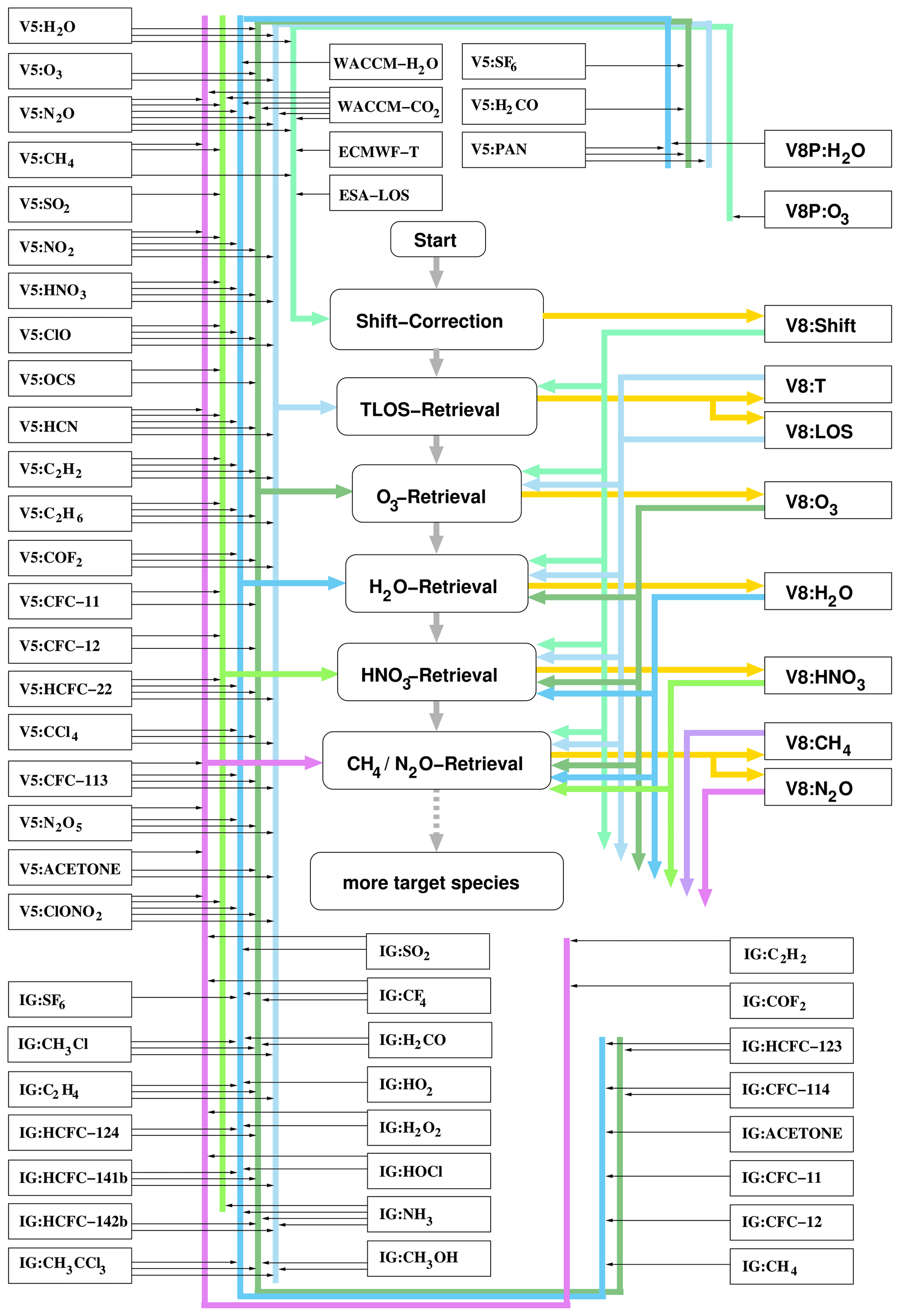
Figure 1 Data flow diagram of the sequential MIPAS processing chain. Mixing ratio information from the MIPAS initial guess database (IG; Kiefer et al., 2002, and updates thereof) is used whenever no V5 or V8 MIPAS results of the related species are available. V8P stands for a preliminary V8 data version.

6.2.1 CO₂ information from model runs

For temperature and tangent altitude retrievals, we use CO₂ mixing ratios calculated with the Whole Atmosphere Community Climate Model (WACCM; Marsh, 2011; Marsh et al., 2013), version 4, run for specified dynamics (García et al., 2017) and uncertainties, as reported by Kiefer et al. (2021). Related TLOS uncertainties are estimated using Eq. (7) with the following:

$$\begin{array}{}\text{(10)}& {\mathit{F}}_{\text{perturbed}}=\mathit{F}(\mathit{T}\mathit{L}\mathit{O}\mathit{S};{\mathit{b}}_{{\mathrm{CO}}_{\mathrm{2}}}+\mathrm{\Delta }{\mathit{b}}_{{\mathrm{CO}}_{\mathrm{2}}}),\end{array}$$

where ${\mathit{b}}_{{\mathrm{CO}}_{\mathrm{2}}}$ and $\mathrm{\Delta }{\mathit{b}}_{{\mathrm{CO}}_{\mathrm{2}}}$ are the CO₂ profiles used and their 1σ perturbations. The perturbation is performed in one step, covering all altitudes. The mixing ratio of the interfering species under assessment is perturbed at all altitudes by 1 σ of its uncertainty at this altitude. As a conservative estimate, all these perturbations are applied with the same sign. This is admittedly not ideal, but we have no more specific correlation information available that would allow for a more adequate approach. Our treatment usually provides an upper estimate of the propagated errors.

For MIPAS measurements of the nominal and UTLS-1 measurement modes, CO₂ mixing ratio uncertainties are deemed to contribute to the random error because, below about 70 km, this error component is thought to be chiefly caused by the natural variability around the climatological value. At altitudes above about 70 km altitude, CO₂ mixing ratio uncertainties are supposed to be dominated by a pronounced systematic component due to model biases, which has to be considered when spectra recorded in the middle and upper atmosphere measurement modes are analysed. No firm statement about related error correlations in the altitude domain can be made.

6.2.2 Abundance information from previous data versions in temperature retrievals

The MIPAS version 5 data product, the predecessor of the current version V8, includes abundance and uncertainty information on many species contributing to the infrared spectrum. The respective abundance information of the limb scan under assessment is used for the interfering species in the forward calculations of the version V8 retrievals. Although broadly considered to be of inferior quality compared to V8 data, the V5 data are considered to be good enough to be used to characterize the small contributions of the interfering species to the signal in the microwindows of the target gas retrieval (Kiefer et al., 2021). While the mapping of the uncertainties in the interfering species was originally estimated using perturbation calculations (Eq. 7), we now use the covariance information S_b;noise that is available from the preceding data retrievals as S_b;meas in Eq. (6). The error components due to uncertainties in the concentrations of interfering species from version 5 MIPAS retrievals contribute chiefly to the random error in the target gas retrieval.

6.2.3 Abundance information from the initial guess database in temperature retrievals

For interfering gases except CO₂ that are not available from preceding MIPAS data versions, the retrievals use mixing ratios from the initial guess database (Kiefer et al., 2002, and updates thereof). Available uncertainty information is vague, and often educated guesses or rational agents' personal beliefs have to be used. Typically, no correlation information is available. Due to this lack of correlation information in the altitude domain, error estimation is approximated by a perturbation calculation using Eq. (7), as described in Sect. 6.2.1.

The capability of the radiative transfer model KOPRA to provide Jacobians with respect to gas concentrations helps to avoid a separate radiative transfer calculation with perturbed concentration data for each trace gas. Instead, the partial derivatives $\frac{\partial y_i}{\partial {\mathrm{vmr}}_{j;g}}$ of spectral radiances y_i with respect to the volume mixing ratio of gas g at altitude j are extracted and used for a linear approximation of the perturbation spectrum F_perturbed,g as follows:

$$\begin{array}{}\text{(11)}& {\mathit{F}}_{\text{perturbed},g}={\mathit{F}}_{\text{nominal}}+\sum _j\mathrm{\Delta }{\mathrm{vmr}}_g,j{\displaystyle \frac{\partial \mathit{y}}{\partial {\mathrm{vmr}}_{j;g}}}.\end{array}$$

In most cases, the resulting error components contribute less than 1 % to the total error budget and therefore are deemed negligible. Since the true errors in this category are most likely even smaller than our estimates, this holds with even greater reason.

For the category of interferents discussed here, no vertical correlation information is available, and all the information given in the context of CO₂ uncertainties applies here too.

We assume that the error in the retrieved quantities caused by using concentrations from a database is dominated by natural variability. That is to say, we assume that the database provides, on average, in the long run, the correct values and that the related error is driven by the difference between the actual state and the mean state. With this supposition in force, related errors contribute to the random error budget. Admittedly, this supposition can be challenged, but the contribution of this category of interferents to the total error budget is so small that a more detailed assessment does not seem justified.

6.3 Calibration uncertainties in temperature retrievals

Under calibration uncertainties we summarize gain calibration uncertainties, radiance offset calibration uncertainties, frequency shift uncertainties, and instrument line shape uncertainties.

6.3.1 Gain calibration uncertainties in temperature retrievals

MIPAS gain calibration relies on reference measurements involving an internal blackbody of known temperature and deep space measurements. Related uncertainties have random and systematic components. The random component includes noise in the blackbody measurements and gain variation between blackbody measurements. The systematic component includes inaccuracies of the calibration blackbody, the errors in the correction of the detector nonlinearity, and the neglect of higher-order artefacts (Kleinert et al., 2018). Table 3 of the paper by Kleinert et al. (2018) allows the calculation of the random and systematic uncertainties separately. Estimated random uncertainties are 0.2 %, 0.2 %, 0.2 %, 0.2 %, and 0.4 % for the MIPAS A band (685–980 cm⁻¹), AB band (1010–1180 cm⁻¹), B band (1205–1510 cm⁻¹), C band (1560–1760 cm⁻¹), and D band (1810–2410 cm⁻¹), respectively. The corresponding systematic uncertainties are 1.1 %, 1.0 %, 1.0 %, 0.3 %, and 0.3 %, respectively. Apparent discrepancies of the values are explained by the fact that the values reported by Kleinert et al. (2018) are to be understood as 2σ uncertainties, while our error estimation is consistently based on 1σ uncertainties.

Contrary to the approach described in Kiefer et al. (2021), the gain calibration error, Δ_gainTLOS, of the temperature and tangent altitude vector, TLOS, is now estimated separately for its random and its systematic component by the application of Eq. (7). The perturbations are the same for all spectra of the limb sequence under assessment. We obtain the following:

$$\begin{array}{}\text{(12)}& \begin{array}{ll}{\mathrm{\Delta }}_{\text{gain}}& \mathit{T}\mathit{L}\mathit{O}\mathit{S}=-\mathbf{G}({\mathit{F}}_{\text{perturbed}}-{\mathit{F}}_{\text{nominal}})\\ & =-\mathbf{G}\left(\left(\mathrm{1}+{\left(\frac{\mathrm{\Delta }y}{y}\right)}_A\right){\mathit{F}}_{\text{nominal}}-{\mathit{F}}_{\text{nominal}}\right),\end{array}\end{array}$$

where F_perturbed are the spectral radiances used for the retrieval, of all involved tangent altitudes, with the gain perturbation applied. The gain uncertainty in the MIPAS A band, which is used for the temperature and tangent altitude retrieval, is represented by the scalar ${\left(\frac{\mathrm{\Delta }y}{y}\right)}_A$. F_nominal are the radiances calculated with the radiative transfer model KOPRA for the actual limb sequence under assessment. Since gain errors affect spectra at all tangent altitudes of a limb scan in the same way, error correlations in the altitude domain are present.

6.3.2 Radiance offset calibration uncertainties in temperature retrievals

On the face of it, it may seem inadequate to consider the calibration uncertainty referring to the radiance offset in the error budget because an offset correction is jointly retrieved along with the target variables (Kiefer et al., 2021). We have to, however, distinguish between two different mechanisms causing offset uncertainty, namely the approximately wavenumber-independent component and the offset noise.

The approximately wavenumber-independent component of the offset uncertainty is caused by a possible offset drift between calibration measurements. This error component is indeed accounted for by the retrieval of the offset correction along with the retrieval of the target quantities because this additive offset correction assumes wavenumber independence within each microwindow (von Clarmann et al., 2003). Thus, this error component does not need to be considered in the error budget.

The situation is different for the noise in the deep space measurements that are used for the radiance offset calibration. This noise has a spectral dependence and is thus not fully corrected for by the offset retrieval mentioned above. It is for this reason that we have updated the error estimation scheme for temperature and tangent altitude retrievals used since the work of Kiefer et al. (2021) to include also the noise component of the offset calibration. It is estimated, using Eq. (5), where S_TLOS;meas is specified as follows:

$$\begin{array}{}\text{(13)}& [{\mathbf{S}}_{\mathrm{y};\mathrm{offset}}{]}_{i;j}={\mathrm{nesr}}_i*{\mathrm{nesr}}_j*r_{i;j},\end{array}$$

where nesr_i and nesr_j are the noise equivalent spectral radiances of the offset measurements at spectral grid points i and j (see Kleinert et al., 2018). Error correlations occur due to apodization, due to the fact that offset calibration measurements are provided at a shorter maximum optical path difference than the scene measurements and because the same offset measurement is used for multiple tangent altitudes. To calculate the respective correlation coefficients r_i;j, first the apodization function is convolved with $\sin (i\mathit{\pi }*c)/(i\mathit{\pi }*c))$, where i is the index of the spectral grid point, and where c is the contrast between maximum optical path differences in the deep space and the scene measurements. For MIPAS full resolution, reduced-resolution bands A–C, and reduced-resolution band D, we have c_FR=0.1, c_RR(AC)=0.2, and c_RR(D)=0.033, respectively. This convolution product is convolved with itself and then normalized such that its maximum is 1. The kth value beside the maximum is used as $r_{i,i\pm k}$. For correlations in the altitude domain, it has to be considered that measurements recorded during a forward movement of the interferometer mirror are all offset calibrated with a deep space measurement with forward movement of the mirror, and backward scene measurements are calibrated with a backward deep space measurement. This implies that measurements at every second tangent altitude rely on the same deep space spectrum for offset calibration. As a consequence, the entry in $[{\mathbf{S}}_{y;\mathrm{offset}}{]}_{i;j}$ is zero when the indices point at an odd and an even tangent altitude but does not depend on the tangent altitude as long as i and j both point at even or both point at odd tangent altitudes. That is to say, the correlation coefficient r_i;j between data points of two odd or two even tangent altitudes is the same for all pairings of the same spectral distance, regardless of whether i and j belong to the same tangent altitude or not.

Although the same offset calibration measurement is used for a couple of scene spectra, causing some error correlations in the time domain, in the long run the offset error contributes to the standard deviation of the differences between two independent measurement systems. Therefore, it is regarded as random error.

6.3.3 Spectral shift uncertainties in temperature retrievals

Prior to the retrievals, a correction of the frequency calibration of the MIPAS spectra is performed for each limb scan, using narrow, isolated lines spread over the entire spectrum covered by MIPAS. A linear model is fitted to the individual spectral shifts determined for each of these lines, providing a linear relation between the spectral shift and wavenumber. The scatter of the individual spectral shifts around the regression line serves as an estimate of the residual frequency correction uncertainty and was found to be 0.00029 cm⁻¹ (Kiefer et al., 2021). The resulting error in the mixing ratio of the target gas is evaluated using Eq. (7), where F_perturbed is an estimate of the spectral radiances for a spectral shift perturbed by the 1σ frequency correction uncertainty, and where F_nominal are the spectral radiances calculated with the nominal frequency correction.

Errors in the retrieved quantities due to the spectral shift uncertainty contribute to the random error. They are fully correlated in the altitude domain.

6.3.4 Instrument line shape uncertainties in temperature retrievals

Errors in the line shape used in the radiative transfer calculation are quantified in terms of modulation efficiency, which is a key input parameter of the instrument line shape model used (Hase, 2003). The propagation of the modulation efficiency error is estimated using Eq. (7), where

$$\begin{array}{}\text{(14)}& {\mathit{F}}_{\text{perturbed}}=\mathit{F}(\mathit{T}\mathit{L}\mathit{O}\mathit{S};e+\mathrm{\Delta }e),\end{array}$$

and where

$$\begin{array}{}\text{(15)}& {\mathit{F}}_{\text{nominal}}=\mathit{F}(\mathit{T}\mathit{L}\mathit{O}\mathit{S};e).\end{array}$$

The scalar e is the nominal modulation efficiency and Δe its perturbation by 1σ.

Spectral shift errors caused by instrument line shape errors do not need to be considered to be part of the instrument line shape error because the total spectral shift is empirically corrected as the first step of the data processing chain (see Fig. 1) and the residual spectral shift uncertainty is propagated as an error source in its own right (see Sect. 6.3.3).

Since the modulation efficiency parameter is based on a pre-flight study and used for all MIPAS retrievals, the related error in the target mixing ratio profile is systematic and fully correlated in the altitude domain.

6.4 Uncertainties in spectroscopic data in temperature retrievals

The leading components of uncertainties in spectroscopic data are line intensity uncertainties and uncertainties in the broadening coefficients. Both error sources are evaluated independently. The fact that no correlation information on spectroscopic uncertainties is available is a major drawback. For most retrievals from MIPAS data, multiple lines are used. If the intensity errors in multiple lines were uncorrelated, e.g. because they are dominated by measurement noise in the lab measurements, then their effect would partly average out in a multi-line retrieval. Conversely, if the intensity errors were strongly correlated, e.g. because they are caused by uncertainties in the amount of gas in the cell in the laboratory measurement, then their effect would be systematic and thus survive the implicit averaging taking place in a multi-line retrieval. Similar considerations hold for the broadening coefficients. Since we have no better information, we consider the spectroscopic uncertainties to be fully correlated. This assumption is conservative with respect to the error budget of the target but optimistic insofar as the error compensation in the context of entangled errors may be overestimated. Since the same spectroscopic parameters are used for all MIPAS retrievals of a certain target gas, related concentration errors contribute chiefly to the systematic error budget. They are fully correlated in the altitude domain insofar as the same microwindows are used for all altitudes.

6.4.1 Line intensity uncertainties in temperature retrievals

The response of the retrieval of temperature and tangent altitudes to errors in CO₂ line intensities is estimated by perturbation using Eq. (7). F_perturbed are the spectral radiances calculated with the intensities of all CO₂ lines of the target gas, which are all perturbed by 1 σ of their individual uncertainty, where all perturbations have the same sign. F_nominal are the spectral radiances calculated with the nominal line intensities.

6.4.2 Broadening coefficient uncertainties in temperature retrievals

All the information given for the propagation of line intensity uncertainties holds, with all necessary changes in place, also for the uncertainties in broadening coefficients. For the evaluation of the error component due to the target gas broadening coefficients according to Eq. (7), we calculate F_perturbed with the broadening coefficients of the target gas, all perturbed by 1 σ of their individual uncertainty, where all perturbations have the same sign.

7 Error components of the trace constituents retrieval

For MIPAS trace gas retrievals, the following error sources are considered: measurement noise, uncertainties in temperature and pointing information (TLOS), and uncertainties in the mixing ratios of interfering species, which contribute in a sizeable way to the signal in the analysis window(s) of the target species and are not jointly fitted with the target gas. Under certain conditions, smoothing error crosstalk can also be an issue. Further error sources under consideration are gain, offset, and frequency calibration errors, as well as instrument line shape uncertainties, uncertainties in spectroscopic data in terms of line intensity and broadening coefficients, and, if applicable, uncertainties in specific parameters to non-local thermodynamic equilibrium (non-LTE), such as kinetic rate constants or abundances of trace gases that interact via specific non-LTE processes rather than by spectral interference. In the following sections, the related error propagation schemes are discussed.

7.1 Measurement noise in the trace constituents retrieval

Noise in retrieved trace gas abundance x is calculated by Gaussian error propagation, using the same method as discussed for the temperature retrieval in Sect. 6.1. The noise error covariance matrix S_x;noise of the target gas profile x is calculated from the gain matrix of the retrieval, G, and the measurement noise covariance matrix, S_y;noise, using generalized Gaussian error propagation (Eq. 5). Again, we use for MIPAS error estimation the following variant of this equation:

$$\begin{array}{}\text{(16)}& {\mathbf{S}}_{x;\mathrm{noise}}={\mathbf{A}}_x({\mathbf{K}}_x^T{\mathbf{S}}_{y;\mathrm{noise}}^{-\mathrm{1}}{\mathbf{K}}_x+{\mathbf{R}}_x{)}^{-\mathrm{1}}.\end{array}$$

All details mentioned in the context of the mapping of measurement noise on temperature also applies to trace gas retrievals. The only relevant error correlations refer to the altitude domain within one profile and between mixing ratios of different species that are retrieved in one step, as done, for example, for CH₄ and N₂O; related correlation information is provided by the off-diagonal elements of S_x;noise. No correlations across limb scans or between sequentially retrieved atmospheric constituents have to be considered.

7.2 Propagation of temperature and pointing errors

Temperature and pointing retrieval errors propagate onto the trace gas retrievals. Temperature and pointing retrieval errors are correlated. These correlations – and correlations in the altitude domain – have to be considered for the error estimation of trace species. The error components of TLOS are, along with the respective correlation information, represented by the covariance matrix S_{TLOS;component}.

Some components of the temperature and pointing errors contribute to entangled errors. Thus, the respective error components contributing to the temperature and pointing error have to be propagated separately for the different sources of TLOS errors. Some of these components contribute to the random error, and others contribute to the systematic error. For this reason, we report them component-wise. The following temperature and pointing error components are considered: measurement noise, gain calibration uncertainty, offset calibration uncertainty, frequency calibration errors, and uncertainties in spectroscopic data.

7.2.1 Propagated temperature and pointing noise

The mapping of noise on temperature and pointing information is characterized by the covariance matrix S_{x;TLOS_random} and is evaluated with Eq. (6), where S_b;meas is specified as S_TLOS;noise. This error covariance matrix represents the noise component of the retrieved temperatures and tangent altitudes of the limb sequence under evaluation. Here we do not need the full covariance matrix of the temperature and pointing retrieval but only those blocks which refer to temperature and tangent altitude information. Entries related to the background continuum and gases fitted jointly with temperature and tangent altitudes play no role here. The entries of S_TLOS;noise are available as a byproduct of the temperature and tangent altitude retrieval. Due to their correlated nature, temperature and pointing/tangent altitude errors have to be propagated jointly rather than separately.

K_b in Eq. (6) is specified as the Jacobian K_TLOS representing the sensitivities of the radiance in the analysis windows of the target gas with respect to changes in temperatures and tangent altitudes. K_TLOS is not the same as the Jacobian used in the temperature and pointing retrieval because it refers to the spectral radiances in the microwindows used for the retrieval of the target gas x.

Temperature and pointing noise contribute to the random error in the target gas retrieval in the sense that it is uncorrelated across limb scans. Resulting trace gas errors are correlated in the altitude domain and also across species. That is to say, if, due to a temperature assumed too low, too high mixing ratios are retrieved for one species, then the mixing ratio of another species is also likely to be retrieved too high.

7.2.2 Propagated temperature and tangent altitude errors due to spectral shift

A correction of the supposedly less-than-perfect frequency calibration of the spectra is performed prior to the retrieval of temperature and tangent altitudes, as described in Kiefer et al. (2021). These authors also provide estimates of the response of the retrieved temperatures and tangent altitudes to the estimated residual frequency calibration error (see Sect. 6.3.3). Again, the response Δ_TLOS;shiftx of the retrieval of trace gas profile x to the temperature and pointing uncertainty due to the spectral shift uncertainty is estimated by the perturbation approach using Eq. (7), where F_perturbed are the spectral radiances obtained with a radiative transfer calculation using temperatures and pointing perturbed by Δ_shiftTLOS, and where F_nominal are the spectral radiances obtained with the spectral shift used for the retrieval.

$$\begin{array}{}\text{(17)}& \begin{array}{rl}{\mathrm{\Delta }}_{\text{TLOS;shift}}\mathit{x}& =-\mathbf{G}\left(\mathit{F}(\mathit{x};\mathit{T}\mathit{L}\mathit{O}\mathit{S}+{\mathrm{\Delta }}_{\text{shift}}\mathit{T}\mathit{L}\mathit{O}\mathit{S})\right.\\ & \left.-\mathit{F}(\mathit{x};\mathit{T}\mathit{L}\mathit{O}\mathit{S})\right).\end{array}\end{array}$$

Since temperature and pointing information in terms of tangent altitudes are jointly retrieved in one inversion step, errors in these quantities are correlated, and perturbations are made in one step. Δ_shiftTLOS vectors are available from Kiefer et al. (2021), who evaluated this quantity for the representative atmospheric conditions listed in Sect. 5 by perturbation studies. Since the spectral shift correction is performed for each limb scan separately, all related errors contribute to the random error budget. And since the spectral shift correction provides only one scalar value per limb scan and microwindow, the resulting target mixing ratio errors are fully correlated in the altitude domain, as follows:

$$\begin{array}{}\text{(18)}& {\text{covar}}_{\text{shift-tlos};i,j}={\mathit{\sigma }}_{\text{shift-tlos};i}{\mathit{\sigma }}_{\text{shift-tlos};j},\end{array}$$

where ${\text{covar}}_{\text{shift-tlos};i,j}$ is the covariance between the errors in the target species due to the propagated shift-induced temperature and pointing errors, σ_shift-tlos, at altitude levels i and j. All the information given about error correlations due to temperature and pointing noise also applies to temperature and tangent altitude errors due to spectral shift.

7.2.3 Propagation of temperature and tangent altitude errors due to offset calibration uncertainties

Retrieved temperatures and tangent altitudes are susceptible to offset calibration uncertainties (see Sect. 6.3.2). The relevant component of the offset uncertainty that is not removed by joint-fitting the offset along with the target variables is dominated by noise in the deep space measurements. Related temperature and pointing errors propagate onto the error budget of the target species. Their contribution is estimated using Gaussian error propagation, according to Eq. (6), where K_b is the sensitivity of the radiances used for the retrieval of the target gas to temperatures and tangent altitudes, and where S_b;meas=S_TLOS;offset, i.e. the covariance matrix of temperature and pointing errors due to offset uncertainties. S_TLOS;offset has relevant off-diagonal entries for the following reasons: (1) offset measurements use interferograms with a shorter maximum optical path difference than the scene spectra but are finally zero padded to the length of the scene interferograms (corresponding to a Fourier interpolation in the spectral domain to achieve the same sampling as the scene spectra), (2) apodization is applied, and (3) offset measurements are used for multiple tangent altitudes. The offset noise variances are calculated from the noise equivalent spectral radiances, as shown in Fig. 8 of Kleinert et al. (2018). Since the offset uncertainties vary randomly in the wavenumber domain, and since the spectral analysis windows of temperature along with pointing are generally different from those used for the retrieval of the target species, this particular calibration uncertainty does not fall into the category of entangled errors but can be treated as an independent error component. This error component contributes, in the long run, to the random error in the target gas because it causes a scatter rather than a bias when compared to independent data from other instruments. Within shorter timescales between two offset calibration measurements (less than 300 s for FR measurements and less than 700 s for RR measurements), positive error correlations have to be expected (Kleinert et al., 2018, their Table 3). This error is also positively correlated in the altitude and across different species.

7.2.4 Propagated temperature and tangent altitude errors due to gain calibration and spectroscopic data uncertainties

Further error components contributing to the temperature and pointing random error are gain calibration uncertainties (Sect. 6.3.1) and uncertainties in the spectroscopic data used (Sect. 6.4). On the supposition that spectroscopic data errors are fully correlated in the spectral domain, related propagated temperature and tangent altitude errors fall in the category of entangled errors and are discussed along with the respective direct propagation of CO₂ spectroscopic uncertainties onto the target gas retrieval (Sect. 7.5).

If the target gas is chiefly retrieved in the MIPAS A band, used for the temperature and tangent altitude retrieval, then propagated temperature and tangent altitude errors due to gain calibration also belong in the category of entangled errors and are discussed along with the directly propagated gain calibration errors (Sect. 7.4.1). The situation is different if the target gas is retrieved in another MIPAS band. The dominant gain error components (especially those caused by nonlinearity) are correlated only within MIPAS bands but not between MIPAS bands (Kleinert et al., 2018). This implies that propagated gain calibration errors in temperature and tangent altitudes are uncorrelated with the gain calibration error in the target gas and have thus to be treated as independent error components. In this case, the propagation of the gain-related temperature and tangent altitude error in the target gas concentration is estimated with Eq. (7), where

$$\begin{array}{}\text{(19)}& {\mathit{F}}_{\text{perturbed}}=\mathit{F}(\mathit{x};\mathit{T}\mathit{L}\mathit{O}\mathit{S}+{\mathrm{\Delta }}_{\text{gain}}\mathit{T}\mathit{L}\mathit{O}\mathit{S}).\end{array}$$

Trace gas errors due to gain-related temperature errors are considered to be positively correlated across species, across altitudes, and across limb scans.

7.3 Uncertainties in interfering species

Uncertainties in interfering species, i.e. species that contribute to the signal in the microwindows of the target gas, have, broadly speaking, a small impact on the retrieved mixing ratios of the target species. This is because (a) the microwindows have been defined such that the signal of interfering species is minimized, (b) the sequence of operations is such that the abundances of strong emitters are retrieved first and are thus available when weak emitters are analysed, (c) for most interfering species, retrieved mixing ratios for the actual conditions are available from earlier MIPAS data versions, and (d) in cases of an appreciable influence of the interfering gas on the retrieved profile of the target gas, the interfering gas is jointly fitted with the target gas and thus does not contribute to the parameter error budget but is accounted for already in the noise covariance matrix of the combined target–interferent retrieval. Nevertheless, the propagation of the uncertainties in interfering species is considered. The error estimation schemes used depend on the source of the information on the interfering species. Sources of information on these constituents' abundances and their uncertainties are as follows:

1. preceding retrievals in the sequential retrieval chain,

2. MIPAS version 5 data, and

3. the MIPAS initial guess database.

In the following, the error propagation for these cases is discussed. If a certain constituent is a strong interferent, that is to say, it causes a large signal in the microwindows of the target gas, then occasionally this constituent is fitted jointly with the target gas. In some cases, this approach is chosen even if the abundance is already known from a preceding retrieval step. The reason behind this approach is to avoid spectral residuals caused by spectroscopic inconsistencies between the microwindows where the interfering constituent has been retrieved and the microwindows where the target gas is retrieved. In this case, the effect of the interferent chiefly is that its consideration in the retrieval slightly increases S_x;noise, and no extra treatment of the interferent is needed in the error budget. In these joint retrievals, the regularization of the interferent is chosen to be sufficiently weak to ignore any smoothing error crosstalk between the interferent and the target gas.

For interfering gases that were not jointly fitted along with the target gas, the error components are evaluated for each gas separately. The only exception are gases which were jointly retrieved in a preceding retrieval, where, therefore, inter-gas covariances have to be considered.

7.3.1 VMR information from preceding retrievals

MIPAS spectra contain contributions of tens of different species. The simultaneous inversion that provides all these mixing ratio profiles in one single inversion is not practicable. Instead, the retrieval is decomposed into a series of retrievals, each providing information on typically only one, occasionally a few, species and each using spectral microwindows which contain the largest possible amount of information on the target gas, while contributions by interfering gases are kept small. The retrieval chain is organized in a way that first the mixing ratio profiles of those trace gases are retrieved that make major signal contributions to the spectrum. When the retrieval of the abundances of minor contributors follows later in the retrieval chain, the concentrations of those gases retrieved earlier in the retrieval chain are already known. Also, their noise covariance matrix is available from the preceding retrievals and is used to analyse the error propagation onto the target gas profile, using Eq. (6).

The parameter error covariance matrix S_b;noise is specified as that block of the resulting covariance matrix from the preceding retrieval that refers to the profile of the interfering gas. In cases when two interfering species were jointly retrieved in the preceding steps, both related blocks and the respective covariance blocks are needed. Other entries of the covariance matrix of the preceding retrieval need not be considered here because the entries of the Jacobian K_b operating on them would be zero anyway. This Jacobian is specified in this application to represent the sensitivities of the spectral radiances used for the target gas retrieval to the abundances of the interfering species.

Other uncertainties in the gas concentrations from preceding retrievals (due to the gain error, spectroscopic data uncertainties, etc.) belong in the category of entangled errors. The direct errors due to the error source under consideration and the propagated error due to the impact of the error under consideration on the retrieved abundance of the interfering species have an opposite sign, which leads to cancellation. Since, due to the way MIPAS data processing is organized, error contributions by interfering species are generally small, any net effects of these entangled errors that may survive the error cancellation are considered to be negligible.

The error components due to uncertainties in the concentrations of interfering species from preceding retrieval steps contribute to the random error in the target gas retrieval because their systematic components do not effectively propagate due to the compensation mechanism of the entangled errors.

Resulting errors are uncorrelated across limb scans and correlated across altitudes according to the entries of the resulting covariance matrix. On the whole, positive correlations of this error component across species sensitive to the error in a certain pre-fitted gas are to be expected, although these correlations will depend largely on the specific sensitivities, profile shapes, etc.

7.3.2 VMR information from MIPAS V5

It is not possible to organize the MIPAS retrievals in a way that all interfering gases are known from retrievals performed earlier in the retrieval chain. Some minor interferences from species that are retrieved only later in the retrieval chain do occur in the microwindows of the target gas. However, earlier MIPAS data versions of these species are often available, e.g. from MIPAS version 5. Also, for these MIPAS retrievals, error covariance matrices S_b;noise are available, which can be used as S_b;meas in Eq. (6). All the information given in Sect. 7.3.1 applies, with all necessary changes in place, also with regard to the propagation of uncertainties in the abundances of interfering species taken from the version 5 MIPAS analysis.

These error components due to uncertainties in the concentrations of interfering species from version 5 MIPAS retrievals also contribute chiefly to the random error in the target gas retrieval. All the information given about the error calculations for propagated V8 mixing ratio errors holds for the propagated V5 mixing ratio errors.

7.3.3 VMR information from the MIPAS initial guess database

For interfering gases not yet retrieved from MIPAS spectra, i.e. neither version 8 nor V5, mixing ratios and uncertainty estimates from the initial guess database are used. All the information given on this issue in the context of temperature and tangent altitude error estimation (Sect. 6.2.2) applies to trace gas error budgets as well. No firm statement on error correlations of this error component can be made because the error characteristics of the information in the initial guess database is unknown.

Assumed uncertainties in CO₂ mixing ratios, however, deserve an extra treatment because they lead to (serious) entangled errors. This is because the retrieval of temperature and tangent altitudes relies on CO₂ lines, which causes an entangled error. The entangled nature of this error component has two consequences. First, the perturbed spectra in Eq. (7) have to be calculated as follows:

$$\begin{array}{}\text{(20)}& \begin{array}{rl}{\mathit{F}}_{\text{perturbed}}& =\mathit{F}\left(\mathit{x};{\mathit{b}}_{{\mathrm{CO}}_{\mathrm{2}}}+\mathrm{\Delta }{\mathit{b}}_{{\mathrm{CO}}_{\mathrm{2}}},\mathit{T}\mathit{L}\mathit{O}\mathit{S}\right.\\ & \left.+{\mathrm{\Delta }}_{{\mathrm{CO}}_{\mathrm{2}}}\mathit{T}\mathit{L}\mathit{O}\mathit{S}\right),\end{array}\end{array}$$

where ${\mathit{b}}_{{\mathrm{CO}}_{\mathrm{2}}}$ and $\mathrm{\Delta }{\mathit{b}}_{{\mathrm{CO}}_{\mathrm{2}}}$ are the CO₂ profiles used and their 1σ perturbations. And, second, the propagation of ${\mathrm{\Delta }}_{\text{VMR}\left({\mathrm{CO}}_{\mathrm{2}}\right)}\mathit{T}\mathit{L}\mathit{O}\mathit{S}$ implies that this error component has to be considered also for the error budget of target species whose microwindows do not contain any sizeable CO₂ signal. As discussed above, for nominal MIPAS measurements, the CO₂ mixing ratio uncertainties are deemed to contribute to the random error, while for MA/UA measurements a systematic component has to be considered.

7.3.4 Smoothing error crosstalk

As already mentioned, in some cases the abundances of interfering species are fitted jointly with those of the target species. This option has been chosen particularly when the abundances of the interfering species pre-retrieved in an earlier step in the retrieval chain do not fit the associated lines in the current target microwindow well. Possible causes for such behaviour are the inconsistencies in the spectroscopic data in the microwindows where the interferents were retrieved and the microwindows of the current retrieval step. The purpose of fitting the interferents again is simply to remove the related spectral residuals and to minimize the related error propagation. Since the microwindows of the current retrieval step include only little information on the interferents, the related results are discarded. They neither supersede nor complement the results from the earlier retrievals when the interferents were the target species.

Due to the limited amount of information on the interferents, their retrieval has to be heavily regularized in some cases. The regularization chosen is a Tikhonov-type smoothing regularization where a squared first-order finite difference operator is included in the cost function (see, e.g., Kiefer et al., 2021, and references therein). Thus, limited information in terms of the degrees of freedom is gained. This is tolerable because the fine structure of the interferent profiles is available from the earlier retrievals, the results of which is used as prior information of the subsequent joint retrieval. That is to say, the fine structure of the vertical profile of the interferent comes from the original retrieval, which is used as prior information and survives the new joint retrieval. In contrast, the information on the total amounts comes from the joint retrieval of the current step. This joint retrieval does not add any appreciable new information on the profile shape of the interferent.

Critical readers might argue that jointly retrieved species can cause an error component of the target species. This is because the regularization of the jointly fitted interferent will affect also the target species via the off-diagonal blocks of the averaging kernel matrix. We call this error component smoothing error crosstalk (von Clarmann et al., 2020). We argue, however, that in most of our cases, the contribution of the smoothing error crosstalk is negligibly small. The reason is that the availability of the fine structure of the profiles from the original retrieval of the interferents is by far sufficient to avoid any related appreciable residuals in the spectra, and the total amount lies in the null space of the Tikhonov regularization matrix block referring to the interferent and thus cannot cause any smoothing error component. In other words, the regularization term in the cost function chosen can only smooth the profile differences $\widehat{\mathit{x}}-{\mathit{x}}_{\mathrm{a}}$ but cannot push them as a whole towards larger or smaller values.

An exception is the joint retrieval of temperature and nitric oxide (NO) from the MIPAS upper atmosphere observations (Funke et al., 2022). In this particular case, information on both retrieval variables, namely temperature and NO above 105 km, is obtained from the same spectral lines of the NO fundamental band at 5.3 µm. Furthermore, no original – and better resolved – retrievals are available a priori for these variables. The impact of the smoothing error crosstalk on the combined temperature and NO retrieval for upper atmospheric observations was extensively investigated by Bermejo-Pantaleón et al. (2011) for MIPAS version V4O retrievals. In particular, these authors showed that the use of inappropriate nighttime NO a priori profiles in this retrieval version led to a pronounced distortion of the retrieved nighttime temperature profiles by up to 50 K in the lower thermosphere. Bermejo-Pantaleón et al. (2011) therefore recommended using the full averaging kernel matrices and a priori vectors (covering the full temperature and NO space and all relevant off-diagonal elements) when model results or correlative measurements are made comparable to MIPAS results. A drawback of this recipe, however, is that temperature and NO information are not always both available from model simulations or correlative measurements. And, even if they were, such comparisons would be difficult to interpret because resulting differences cannot be unequivocally attributed to individual parameters. To overcome these problems and to enable comparisons in single parameter spaces (temperature only or NO concentrations only), we report V8 retrievals crosstalk error estimates that correspond to the mapping of NO a priori uncertainties in the retrieved temperature profile, and vice versa. These error estimates are calculated as $(\mathbf{I}-\mathbf{A}){\mathbf{S}}_{\text{a}}(\mathbf{I}-\mathbf{A}{)}^T$, where I is the identity matrix of the respective dimension (Rodgers, 2000) by using a priori covariance matrices S_a manipulated as follows. For the estimation of the smoothing error crosstalk components due to the constraint on the NO profile in the retrieval, the only non-zero entries in S_a refer to the NO concentrations, while temperature variances and covariances, in addition to covariances between temperature and NO, are set to zero. Conversely, for the estimation of the smoothing error crosstalk due to the temperature constraint, the only non-zero block in S_a is the one which contains the temperature variances and covariances.

7.4 Calibration uncertainties

The same calibration uncertainties discussed in the context of the temperature and tangent altitude retrieval (Sect. 6.3) are also relevant to the retrieval of trace gas abundances. These are gain calibration errors, radiance offset calibration errors, frequency shift uncertainties, and instrument line shape uncertainties.

7.4.1 Gain calibration uncertainties

In a similar manner as for the temperature and tangent altitude error estimation, the propagation of the random and systematic gain calibration uncertainties in the retrieved trace gas abundances are also estimated using perturbation studies with the following:

$$\begin{array}{}\text{(21)}& {\mathrm{\Delta }}_{\text{gain}}\mathit{x}=-\mathbf{G}({\mathit{F}}_{\text{perturbed}}-{\mathit{F}}_{\text{nominal}}).\end{array}$$

Gain calibration errors come into play in trace gas retrievals via two different pathways. First, they affect the trace gas retrieval directly. And, second, they affect the trace gas retrieval via the propagation of the gain error in temperature and tangent altitudes. We have to distinguish between three different cases. The retrieval of the target gas under assessment uses (1) only spectral lines in the MIPAS A band, where TLOS has been retrieved, (2) only spectral lines in MIPAS bands AB to D, and (3) spectral lines both in the A band and in other bands.

If the target gas is retrieved in the MIPAS A band (case 1), where temperature and tangent altitudes are also retrieved, gain and gain-induced temperature and tangent altitude errors belong in the category of entangled errors. We take this into account by calculating F(perturbed) with temperature and pointing perturbations as resulting from the error estimation of the combined temperature and tangent altitude retrieval, using the following:

$$\begin{array}{}\text{(22)}& \begin{array}{rl}{\mathit{F}}_{\text{perturbed}}& =\left(\mathrm{1}+{\left({\displaystyle \frac{\mathrm{\Delta }y}{y}}\right)}_A\right)\mathit{F}\left(\mathit{x};\mathit{T}\mathit{L}\mathit{O}\mathit{S}\right.\\ & \left.+{\mathrm{\Delta }}_{\text{gain}}\mathit{T}\mathit{L}\mathit{O}\mathit{S}\right).\end{array}\end{array}$$

TLOS represents the vector representing the temperature profile and the tangent altitudes retrieved in the preceding step and is used for the target gas retrieval, and Δ_gainTLOS is the vector containing the responses of the retrieved temperature profile and tangent altitudes to a positive gain perturbation.

For target gases retrieved in any band other than the MIPAS A band (case 2), this entanglement mechanism does not apply. In this case, the target gas error component due to the gain calibration error is calculated as follows:

$$\begin{array}{}\text{(23)}& {\mathit{F}}_{\text{perturbed}}=\left(\mathrm{1}+\mathrm{\Delta }\mathit{y}/\mathit{y}\right)\mathit{F}\left(\mathit{x}\right).\end{array}$$

This error component and the mapping of the gain-related temperature and tangent altitude error, as estimated with the perturbation approach as defined in Eq. (19), are treated as independent errors. If the retrieval uses lines from multiple MIPAS bands AB, B, C, or D, then it is adequate to consider both the systematic and the random components of the gain calibration error in the different bands as independent errors. This is because the random and systematic components of the gain calibration error are dominated by components that are highly correlated only within a MIPAS band but uncorrelated between the bands. This implies that, for both the systematic and the random component, a perturbation calculation is needed for each band involved.

The situation is more complicated in cases where spectral lines both in the MIPAS A band and one or more of the other bands are used (Case 3). For both the systematic and the random part of the gain error estimate, the following approach is used. The perturbed spectrum is calculated using Eq. (22), but the $\mathrm{\Delta }\mathit{y}/\mathit{y}$ term is applied only to radiances in the MIPAS A band. The error component calculated with this perturbation spectrum accounts for the propagated gain-induced temperature and tangent altitude error and the gain error in the A band. Systematic and random components of the error due to gain calibration uncertainties in the other bands are estimated using Eq. (23) for each band separately.

Mixing ratio errors due to propagated gain calibration uncertainties are positively correlated in the altitude domain, across species, and, to a large extent, also across limb scans.

7.4.2 Radiance offset calibration uncertainties

The treatment of radiance offset calibration uncertainties in the error estimation of trace gas retrievals follows exactly the scheme presented for temperature and tangent altitude retrievals in Sect. 7.2.3. Since the relevant components of the radiance offset calibration uncertainty are independent between different spectral regions, and since the microwindows for trace gas retrievals are different from those used for the temperature and tangent altitude retrievals, these radiance-offset-related errors do not fall into the category of entangled errors. This error component contributes to the random error budget, although short-term correlations across limb scans have to be considered, as described in Sect. 7.2.3. Correlations in the altitude domain are characterized by the entries of the related covariance matrix. Across species, this error component is usually uncorrelated, except for rare cases where the selected transitions of the different species are spectrally close together.

7.4.3 Spectral shift uncertainties

Trace gas retrieval errors due to spectral shift errors are estimated by perturbation studies in the same way as for the temperature and tangent altitude retrieval (Sect. 6.3.3).

In this context, it should be mentioned that target concentration uncertainties directly caused by spectral shift uncertainties and target concentration uncertainties due to temperature and pointing errors caused by spectral shift uncertainties do not fall in the category of entangled errors. This is because the response of the target concentration to the spectral shift and the response of the target concentration to shift-induced temperature and pointing errors is erratic rather than systematic.

Errors in the retrieved quantities due to the spectral shift uncertainty contribute to the random error, and they are fully correlated in the altitude domain. Across gases, no general statement can be made because correlations depend on the specific conditions. At least it can be assumed that for two gases with lines of similar widths and similar vertical distributions the correlations will more likely be positive than negative.

7.4.4 Instrument line shape uncertainties

As discussed in Sect. 6.3.4, the only relevant instrument line shape parameter to be considered in the error estimation is the modulation efficiency of the interferometer. Its propagation onto the retrieved trace gas abundances is estimated using Eq. (7), where

$$\begin{array}{}\text{(24)}& {\mathit{F}}_{\text{perturbed}}=\mathit{F}(\mathit{x};e+\mathrm{\Delta }e,\mathit{T}\mathit{L}\mathit{O}\mathit{S}+{\mathrm{\Delta }}_{\text{e}}\mathit{T}\mathit{L}\mathit{O}\mathit{S}),\end{array}$$

and where

$$\begin{array}{}\text{(25)}& {\mathit{F}}_{\text{nominal}}=\mathit{F}(\mathit{x};e,\mathit{T}\mathit{L}\mathit{O}\mathit{S}).\end{array}$$

x is the retrieved profile of the target gas for which the perturbations are evaluated. Scalar e is the nominal modulation efficiency and Δe its perturbation by 1 σ. Δ_eTLOS is the response of the temperature and pointing retrieval to a perturbation of e by Δe. Since the direct effect of Δe and its indirect effect via Δ_eTLOS are entangled errors, their perturbations are evaluated in one run of the forward model in order to obtain the compensation effects correctly. This error component contributes to the systematic error, is fully correlated in the altitude domain, and is positively correlated across gases.

7.5 Uncertainties in spectroscopic data

Uncertainties in line intensities and broadening coefficients are fully correlated in the altitude domain, insofar as the same microwindows are used for all altitudes, and they contribute chiefly to the systematic error. The problem of unknown error correlations between different lines of the same gas that has been discussed in Sect. 6.4 also applies to trace gas retrievals. Mixing ratio errors due to errors in spectroscopic data are uncorrelated across species, but correlations in the altitude domain have to be considered.

7.5.1 Line intensities

The response of the retrieval of a target gas to errors in the target gas line intensities is estimated by perturbation using Eq. (7), following the scheme discussed for temperature and tangent altitudes in Sect. 6.4.1. Errors in the intensities of CO₂ lines deserve special attention in this context. There is no systematic coupling mechanism between the intensity-induced target gas error and the intensity-induced temperature and pointing error. Therefore, this error component is estimated independently of the error component due to the uncertain line intensities of the target species. For this purpose, Eq. (7) is also used, where

$$\begin{array}{}\text{(26)}& \begin{array}{rl}{\mathit{F}}_{\text{perturbed}}& =\mathit{F}(\mathit{x};\mathit{L}{\mathit{I}}_{{\mathrm{CO}}_{\mathrm{2}}}+\mathrm{\Delta }\mathit{L}{\mathit{I}}_{{\mathrm{CO}}_{\mathrm{2}}},\mathit{T}\mathit{L}\mathit{O}\mathit{S}\\ & +{\mathrm{\Delta }}_{\text{LI}}\left({\mathrm{CO}}_{\mathrm{2}}\right)\mathit{T}\mathit{L}\mathit{O}\mathit{S}),\end{array}\end{array}$$

and where

$$\begin{array}{}\text{(27)}& {\mathit{F}}_{\text{nominal}}=\mathit{F}(\mathit{x};\mathit{L}{\mathit{I}}_{{\mathrm{CO}}_{\mathrm{2}}},\mathit{T}\mathit{L}\mathit{O}\mathit{S}).\end{array}$$

$\mathit{L}{\mathit{I}}_{{\mathrm{CO}}_{\mathrm{2}}}$ are the intensities of the CO₂ lines affecting the signal in the microwindows of the target gas. $\mathrm{\Delta }\mathit{L}{\mathit{I}}_{{\mathrm{CO}}_{\mathrm{2}}}$ is the vector of intensity perturbations, all with the same sign but with an individual amount. ${\mathrm{\Delta }}_{\text{LI}\left({\mathrm{CO}}_{\mathrm{2}}\right)}\mathit{T}\mathit{L}\mathit{O}\mathit{S}$ is the response of the temperature and pointing retrieval to CO₂ line intensity perturbations by 1σ. The perturbation is made for the entire TLOS vector in one step, where the signs of the Δ_LI(CO₂)TLOS components are considered. Due to the entangled nature of the effects of $\mathrm{\Delta }\mathit{L}{\mathit{I}}_{{\mathrm{CO}}_{\mathrm{2}}}$ and Δ_LI(CO₂)TLOS, F_perturbed is evaluated for both of these effects in one step.

Contrary to temperature and tangent altitude information, errors in pre-retrieved concentrations of interfering gases affect only the signal in the lines of these interfering gases. Here the compensation mechanism discussed in Sect. 4.4 takes place in full. A too high line intensity of the interfering line will typically cause a too low mixing ratio of the interferent, and the combination of both these error components will produce a signal of the interfering line fairly close to the true signal. Therefore, we do not consider the line intensity errors in the interfering species in the error budget of the target species.

7.5.2 Broadening coefficients

The propagation of uncertainties in the broadening coefficients onto trace gas mixing ratios follows the scheme described in the previous section for line intensities. Here the entangled nature of the temperature and tangent altitude errors due to uncertainties in broadening coefficients of CO₂ lines also has to be taken into account.

For the evaluation of the propagation of temperature and pointing uncertainties due to CO₂ broadening coefficients according to Eq. (7), we use the following:

$$\begin{array}{}\text{(28)}& \begin{array}{rl}{\mathit{F}}_{\text{perturbed}}& =\mathit{F}\left(\mathit{x};{\mathit{B}}_{{\mathrm{CO}}_{\mathrm{2}}}+\mathrm{\Delta }{\mathit{B}}_{{\mathrm{CO}}_{\mathrm{2}}},\mathit{T}\mathit{L}\mathit{O}\mathit{S}\right.\\ & \left.+{\mathrm{\Delta }}_{\text{B(CO2)}}\mathit{T}\mathit{L}\mathit{O}\mathit{S}\right)\end{array}\end{array}$$

and

$$\begin{array}{}\text{(29)}& {\mathit{F}}_{\text{nominal}}=\mathit{F}(\mathit{x};{\mathit{B}}_{{\mathrm{CO}}_{\mathrm{2}}},\mathit{T}\mathit{L}\mathit{O}\mathit{S}),\end{array}$$

where ${\mathit{B}}_{{\mathrm{CO}}_{\mathrm{2}}}$ are the relevant broadening coefficients of the CO₂ lines involved, $\mathrm{\Delta }{\mathit{B}}_{{\mathrm{CO}}_{\mathrm{2}}}$ is the respective vector of the perturbations, and Δ_B(CO2)TLOS is the net response of the temperature and pointing retrieval to perturbations of CO₂ broadening coefficients.

For reasons discussed in the previous section, estimated errors in the pre-retrieved interferents due to uncertainties in the broadening coefficients are not considered.

8 Further sources of error

In this paper, we concentrate on the assessment of error components that are relevant to temperature, tangent altitudes, and all species retrieved from MIPAS spectra. For the retrieval of products from non-nominal observation modes, and some gases, observation-mode-specific or gas-specific uncertainties may be relevant, in particular, if non-LTE is considered. The assessment of these uncertainties will be discussed in the corresponding retrieval papers, where relevant. The same holds for error sources not discussed so far, such as inaccurate line shape models. The relevance of such effects is deemed highly dependent on the target gas under analysis. The assessment of these uncertainties will either be based on Eq. (7) or simply on sensitivity studies, where the results of retrievals using different retrieval set-ups are compared.

9 A case study: ozone

The error propagation approach presented above is discussed using an ozone retrieval from a MIPAS nighttime measurement at 40.09^∘ N, 11.28^∘ E during Envisat orbit 38517 on 12 July 2009 as a case study. Details of the underlying retrieval procedure are reported by Kiefer et al. (2022). The resulting error components for selected altitudes are presented in Fig. 2 and Table B1.

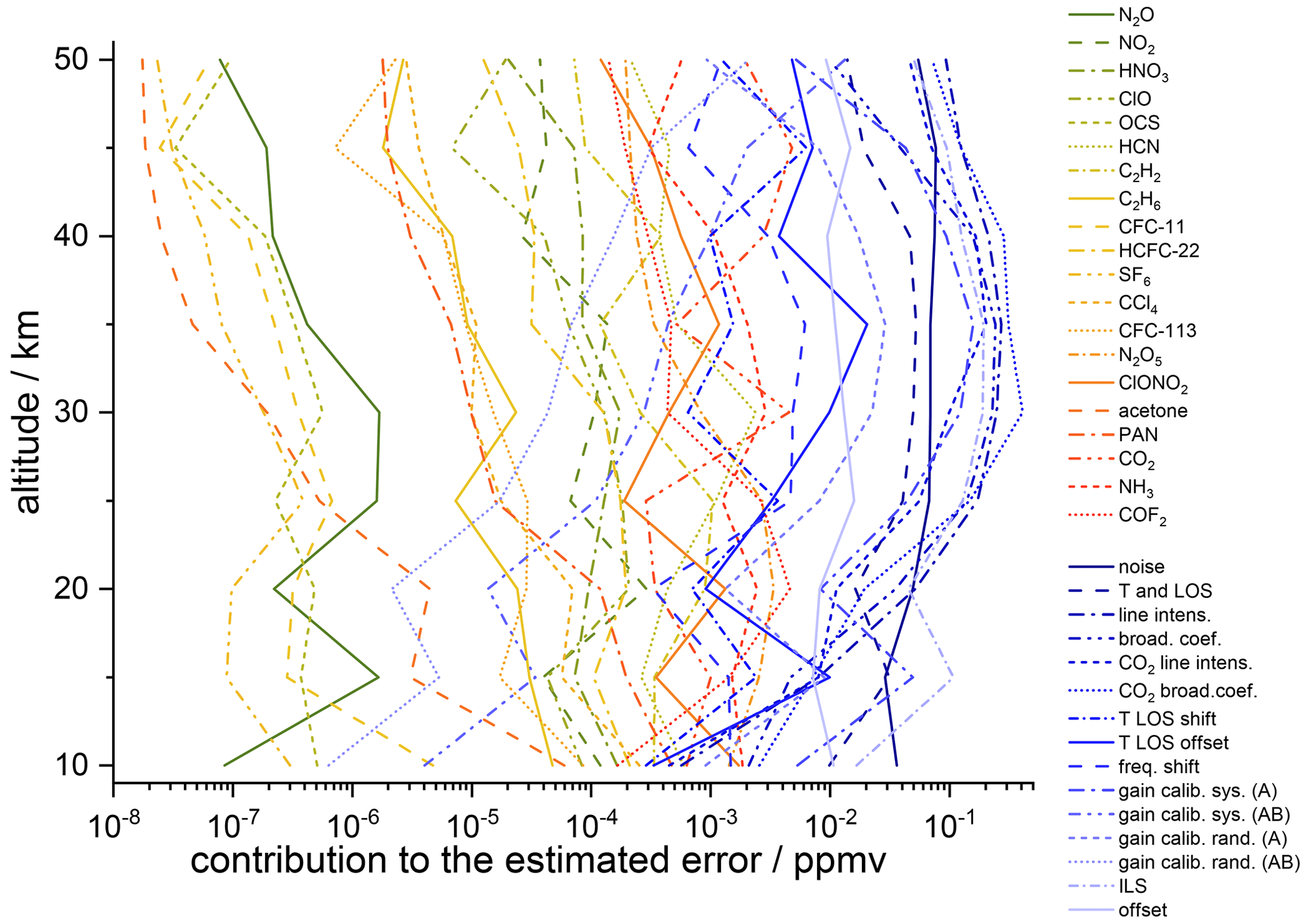
Figure 2 The error budget (absolute values) of a MIPAS ozone retrieval from a limb scan recorded at 40.09^∘ N, 11.28^∘ E during Envisat orbit 38517 on 12 July 2009 at 21:28 UT.

Since a large number of strong ozone lines is available for the retrieval, noise makes only a moderate contribution to the error budget of MIPAS ozone. Instead, the error budget is driven by uncertainties in spectroscopic data, namely line intensities and broadening coefficients. Both spectroscopic data uncertainties in the target gas ozone and those of CO₂ are important. The latter affect the ozone retrieval mainly via tangent altitude errors which propagate onto the ozone retrievals. Furthermore, considerable errors are caused by calibration uncertainties, associated both with gain and offset calibration. Calibration uncertainties related to the MIPAS A band have a much larger effect on the ozone retrieval than those related to the AB band, simply because the majority of spectral lines used for the ozone retrieval are situated in the MIPAS A band (Kiefer et al., 2022). Moreover, instrument line shape (ILS) and tangent altitude (LOS) uncertainties make considerable contributions to the MIPAS ozone error budget.

Broadly speaking, spectroscopic uncertainties along with instrument and calibration-related as well as uncertainties in temperature and pointing information outweigh uncertainties in the abundances of interfering species by far. None of these uncertainties exceeds the contribution of measurement noise.

10 Representative error estimates

Since it is hard to decide a priori which limb scans are representative of a certain typical atmospheric situation, error estimates are calculated for a large number of observations, as discussed in Sect. 5. The representative errors are estimated differently for errors inferred using Gaussian error propagation (Eqs. 5 or 6) and errors estimated using perturbation studies (Eq. 7).

For errors estimated via Gaussian error propagation, the variances – and, if available, also the covariances – are averaged over all limb scans assigned to a given scenario. Since atmospheric state variables retrieved from MIPAS spectra are represented on a fixed altitude grid, independent of the tangent altitudes of the measurement, this step does not involve any interpolation. The result is one mean variance profile per error component and per scenario. For error components where covariance information is available, the respective covariance matrices are averaged. All these error components are regarded as random error components.

Estimates of random error components resulting from perturbation studies are obtained by the arithmetical averaging of the responses to the perturbation. To decide if the error component is chiefly additive or chiefly multiplicative, a linear regression is performed using the responses to the perturbation over the mixing ratios. A predominant axis intercept indicates an absolute (i.e. additive) error component, while a pronounced slope indicates a relative (multiplicative) error component. This empirical assessment supersedes the hitherto intuition-based classification of additive versus multiplicative error components.

Due to the headache error problem, the procedure is slightly more complicated for error components that are labelled systematic and evaluated on the basis of perturbation studies because modulation of the error through the randomly varying atmospheric state may add a random component. When no sizeable latitude or time dependency of these errors is observed, the systematic part of the error component under investigation is the mean over all limb scans associated with the scenario under assessment. The information on the random component of the headache error lies in the scatter around the mean error. When a sizeable dependency of any explaining variable (latitude, time, etc.) is found, a parametric model has to be fitted to the individual errors. In this case, the bias then can be estimated for the actual condition with this model, and the information on the random part of the headache error is included in the unexplained variance around this parameterization. The distinction between additive and multiplicative error components is performed on the basis of a linear regression as described above for the random errors. Most of the error sources assessed by perturbation studies result in multiplicative errors; thus, the use of relative rather than absolute errors is adequate for disentangling systematic and random parts of the headache error.

Error covariances of the random components of the headache errors in the altitude domain can be calculated in a straight forward way along with the averaging procedure. These representative error estimates are reported for the particular species under investigation along with the publication of the data product, such as Kiefer et al. (2022) for ozone.

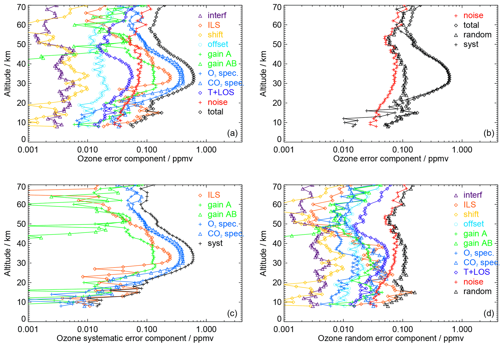
Figure 3 Aggregated estimated ozone errors for the northern midlatitude summer night reference scenario. (a) The total error budget and its components (interf is the interfering species, and ILS is the instrument line shape). (b) The decomposition into random and systematic components. The contributions to the systematic (c) and random (d error budgets. This example was taken from Kiefer et al. (2022).

11 Aggregation of error estimates

Both the total random error estimate and the total systematic error estimate are calculated by adding the respective component error estimates in terms of variances. For this purpose, percentage error estimates are transformed to absolute error estimates using the respective reference concentration profile. Figure 3 shows an example for the northern midlatitude summer night reference scenario. The top left panel shows the error components and the aggregated estimated error (total). In this particular example, it is dominated by spectroscopic uncertainties. The estimated total error variance is the sum of the random error variance and the systematic error variance. The top right panel shows the decomposition of the total error into its aggregated systematic and random components. It is no surprise that the aggregated random error exceeds the uncertainty caused by measurement noise alone. The lower panels show the decomposition of the aggregated systematic (left) and random (right) errors into their components. Except for the lowermost altitudes, uncertainties in spectroscopic data are the leading source of systematic error. It should be mentioned that the estimated bias cannot simply be subtracted from the measurement in order to correct the measurement because the bias estimates are based on perturbation studies with an ad hoc choice of the sign of the perturbation. The systematic uncertainties (instrument line shape, gain calibration, and spectroscopic uncertainties) also contribute to the random error budget and thus appear in both panels, due to their headache-type nature that causes a bias and a scatter around this bias. Below 19 km, the random component of the propagated instrument line shape error even dominates the random error budget. Above this level, measurement noise typically is the leading source of random error.

Since the correlation characteristics in different domains, such as time, altitude, among species, etc., can be different for each error component, there may be cases where it is more adequate to work with the detailed error budget rather than the total error estimates (see, e.g. Kiefer et al., 2022, and references therein).

12 Technical realization

A control program runs over all limb scans associated with the scenario under assessment. For each limb scan, this program calls the radiative transfer model KOPRA for the calculation of the reference spectra F_nominal and the perturbed spectra F_perturbed needed for calculation of error components according to Eq. (7). Furthermore, it provides the gain functions G and covariance matrices S_x,noise of the target species and, as far as available, the covariance matrices S_b,noise of parameter errors and the required Jacobians K_b. With this information on the current limb scan available, the error estimator is called. This program extracts the relevant information from the available covariance matrices S_x,noise and S_b,noise, reads the difference spectra obtained from the perturbed and reference spectra, and estimates the error components of the limb scan under analysis. For each limb scan under consideration, the error estimator provides the error estimates for each error component, based on Eqs. (5)–(7).

Based on the individual estimated error components, a post-processing routine performs all the statistics over the limb scans in the scenario under assessment, including the disentangling of the headache error, as described in Sect. 10. For the reference scenarios, the resulting error estimates are reported, component-wise, random, and systematic, and are deemed representative of the scenario they are assigned to. Our data come with an error class ID (identification code) for each profile that, based on the information provided in Table A6, enables the data user to decide, for any MIPAS measurement, which scenario is applicable. The user who needs only error budgets for the categories of systematic versus random error and absolute versus relative errors does not have to refer to these error class IDs because, for these categories, the related subtotal errors are transformed to and provided for each single observation.

13 Conclusions

This paper presents an overview of an error estimation scheme used for temperatures and trace gas concentrations retrieved from MIPAS spectra with the IMK/IAA data processor. It represents a best effort to make the error reporting compliant with the recommendations by the TUNER activity, as summarized in von Clarmann et al. (2020). In this paper, we limit ourselves to the methodology, insofar as it is overarching over the different data products of MIPAS, to support gas-specific analyses as performed, for example, by Kiefer et al. (2022) for ozone. In particular, the improved separation of systematic versus random error components will foster bias and precision validation, as performed by Laeng et al. (2014), Plieninger et al. (2016), and Eckert et al. (2016) for preceding MIPAS data versions of O₃, CH₄, N₂O, CFC-11, and CFC-12.

Arguably, some error components are not specified as accurately as one would like to have them. This holds true particularly for uncertainties in spectroscopic data, namely line intensities and broadening coefficients. For many species, these uncertainties belong to the leading error sources. The main drawback is that no information on spectroscopic error correlations between the various lines of a gas is provided. The related target gas error largely depends on this correlation. Furthermore, it is a truism that unrecognized or unquantified error sources cannot be considered. Validation studies will show how realistic the estimated random and systematic errors are, how complete the error budget is, and how justified the ingoing assumptions are.

Appendix A: Sample atmospheres

Table A1 Measurements used for error analysis of nominal FR measurements.

Table A2 Measurements used for error analysis of RR nominal measurements.

Table A3 Measurements used for error analysis of middle atmosphere measurements.

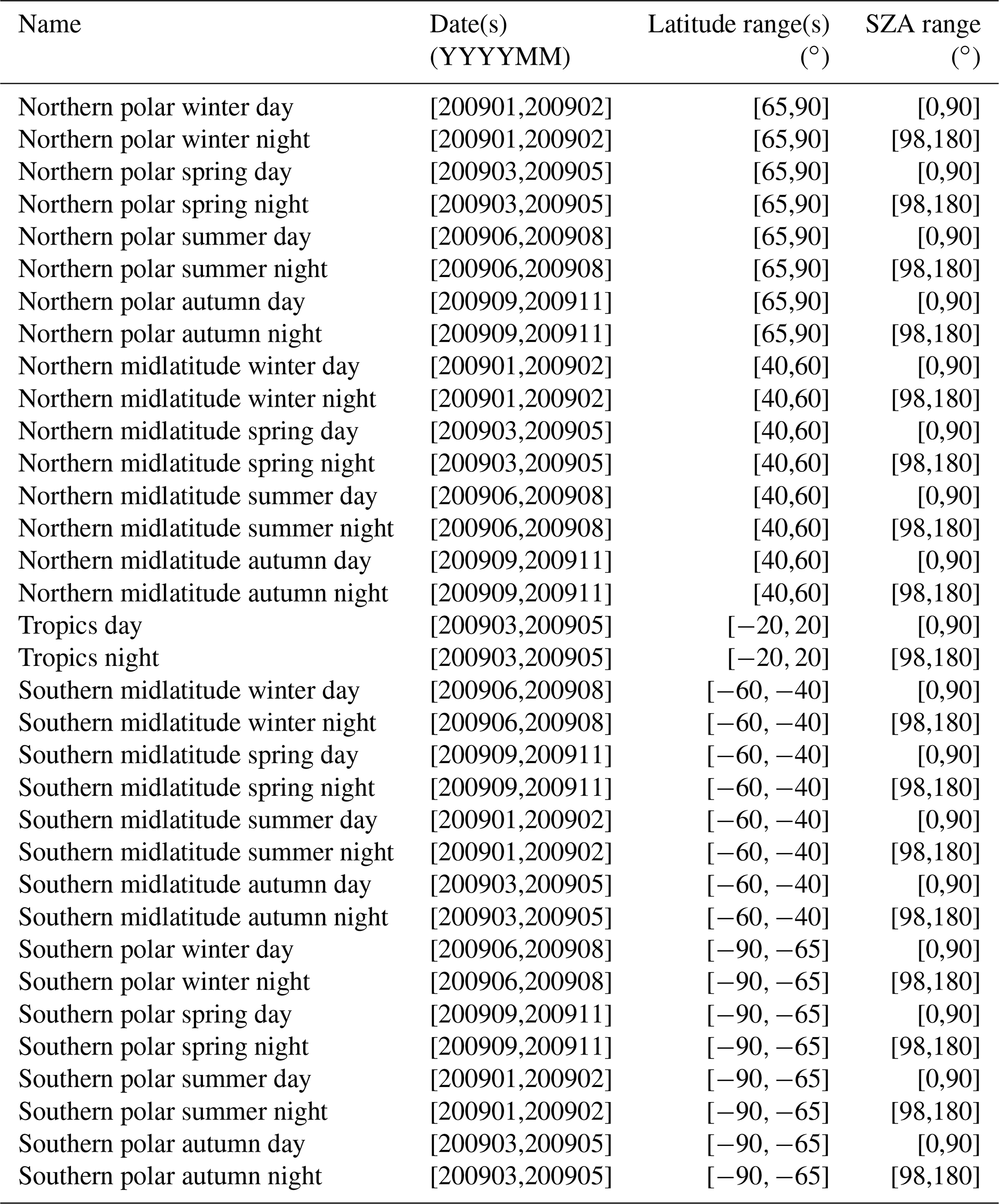
Table A4 Measurements used for error analysis of upper atmosphere measurements and low solar activity.

Table A5 Measurements used for error analysis of upper atmosphere measurements during high solar activity.

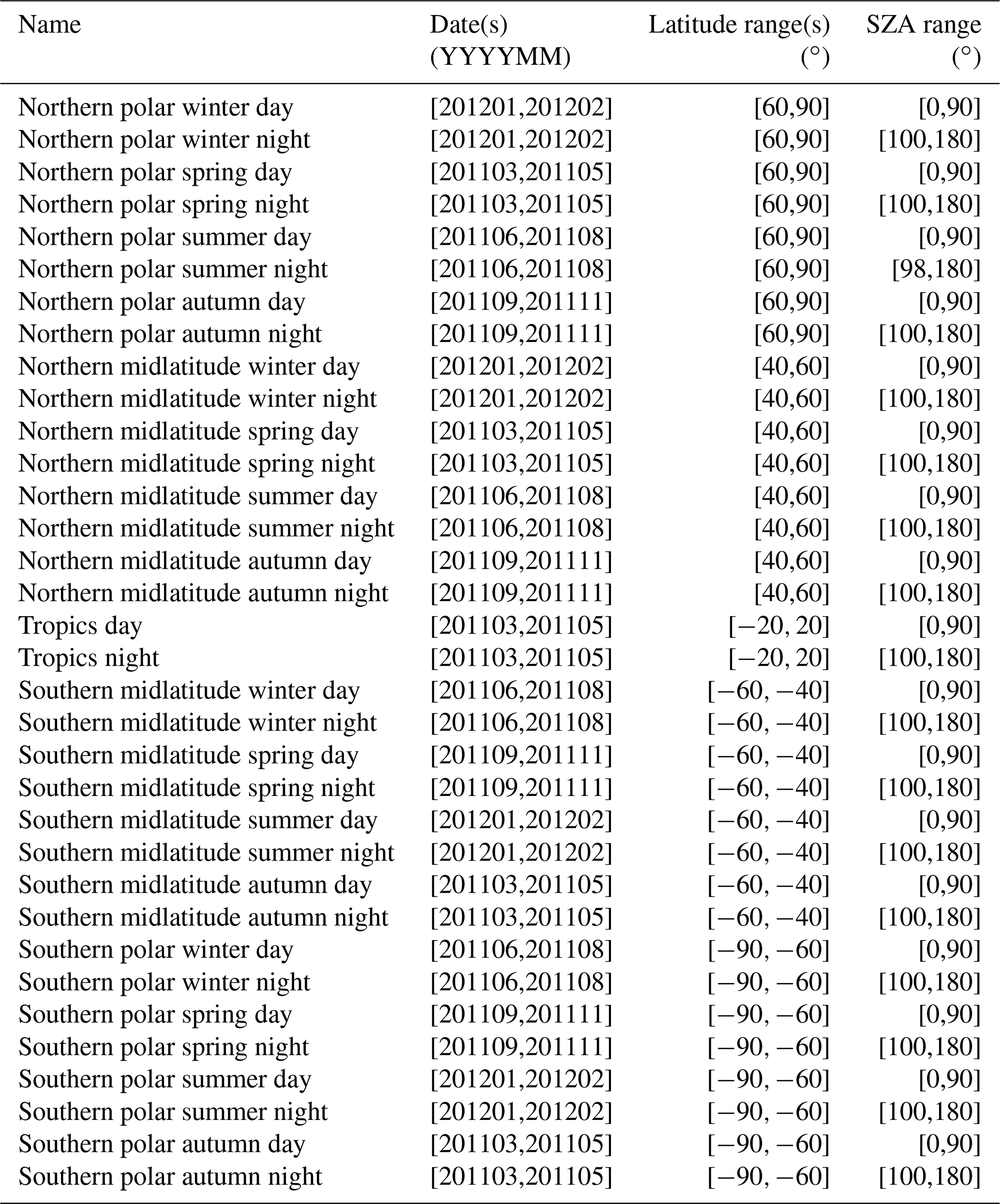
Table A6 Attribution of measurements to scenarios. Note: DJF is December–February, MAM is March–May, JJA is June–August, and SON is September–November.

Appendix B: Case study

Table B1 Estimated errors the ozone retrieval. Note: ppmv is parts per million by volume.