the Creative Commons Attribution 4.0 License.
the Creative Commons Attribution 4.0 License.
 | 09 Dec 2022
Horizontal small-scale variability of water vapor in the atmosphere: implications for intercomparison of data from different measuring systems
Cintia Carbajal Henken
Sergio DeSouza-Machado
Bomin Sun
Tony Reale
Water vapor concentration structures in the atmosphere are well approximated horizontally by Gaussian random fields at small scales (≲6 km). These Gaussian random fields have a spatial correlation in accordance with a structure function with a two-thirds slope, following the corresponding law from Kolmogorov's theory of turbulence. This is proven by showing that the horizontal structure functions measured by several satellite instruments and radiosonde measurements do indeed follow the two-thirds law. High-spatial-resolution retrievals of total column water vapor (TCWV) obtained from the Ocean and Land Color Instrument (OLCI) on board the Sentinel-3 series of satellites also qualitatively show a Gaussian random field structure.
As a consequence, the atmosphere has an inherently stochastic component associated with the horizontal small-scale water vapor features, which, in turn, can make deterministic forecasting or nowcasting difficult. These results can be useful in areas where high-resolution modeling of water vapor is required, such as the estimation of the water vapor variance within a region or when searching for consistency between different water vapor measurements in neighboring locations. In terms of weather forecasting or nowcasting, the water vapor horizontal variability could be important in estimating the uncertainty of the atmospheric processes driving convection.
- Article
(4722 KB) - Full-text XML
- BibTeX
- EndNote


Meteorologists frequently need to determine the water vapor characteristics of an air parcel in the atmosphere. In the review from Wulfmeyer et al. (2015), it is shown how accurate and high-resolution water vapor measurements are indispensable in the understanding and simulation of the water cycle. Unfortunately, it is common to have only partial information for these atmospheric air parcels, usually coming from different measuring instruments or from a numerical weather prediction (NWP) model. As an example, instruments on board satellites usually measure within a big spatial area whose radius is of the order of a few tens of kilometers. On the other hand, ground-based stations or radiosondes measure an extremely small parcel of the atmosphere, which for all practical purposes can be considered “point” measurements. Reconciling all these measurements to make them consistent is not an easy task, and it is what constitutes the point-to-area problem (Loew et al., 2017). There are many examples in which an adequate characterization of water vapor structure in the atmosphere is very useful or critical.
One such examples is passive satellite instruments measuring in the infrared or the microwave region of the spectrum. These instruments measure air-mass regions at horizontal scales of tens of kilometers (i.e., surfaces of a few hundred square kilometers) and vertical thickness of a few kilometers. They actually integrate the radiation coming from all the air sub-parcels into which the measurement region can be subdivided. In fact, the horizontal variability of water vapor within the measurement region in the field of view of satellite instruments can have significant effects when calculating the radiances impinging on the instrument via a radiative transfer model (RTM). In this case, it is necessary to know the variance of the water vapor concentration within the remotely sensed air parcel (Calbet et al., 2018).
Another example is the calculation of instability indices for nowcasting purposes, particularly the convective available potential energy (CAPE). Operational meteorology usually takes as a first approximation of these instability indices the ones obtained from NWP model forecasts or measured from remote sensing satellites. To refine such indices with ground-based station measurements is not simple due to significant differences between different measurements or NWP models (Gartzke et al., 2017). This is caused by the high horizontal variability of water vapor in the atmosphere. To reconcile all estimates of instability indices, it is necessary to properly characterize the temperature and water vapor structure within the air parcel under study.
While it is common to treat atmospheric water vapor as a fluid in turbulent motion in study fields for which measurements are made at small scales, this is usually not so in other areas where larger scales are measured or modeled. Ground station or lidar measurements usually do apply concepts from turbulence theory (Lenschow et al., 2000; Wulfmeyer et al., 2010; Turner et al., 2014; Behrendt et al., 2015). But this is usually not the case in RTM simulations (e.g., Saunders et al., 2018) or NWP modeling (e.g., Milovac et al., 2016). In this paper we will show how, for smaller horizontal scales below ∼ 6 km, the atmosphere does indeed show turbulent behavior. This horizontal scale length can be identified as the outer scale length of turbulence quoted in the literature.
It should be noted that turbulent behavior in the atmosphere can be grouped into two different categories depending on whether the measurement is done mostly in the vertical or the horizontal, each of them involving different scale lengths. The vertical measurements typically have much smaller scale lengths than the horizontal phenomena studied here. Measurements involving mostly vertical variability are typically the scintillation measurements done at low zenith angles (e.g., Townsend, 1965) or turbulence measurements performed with lidars (e.g., Lenschow et al., 2000). They usually quote an outer scale length of turbulence of a few tens to hundreds of meters. On the other hand, measurements involving mostly horizontal features, such as the ones presented in this paper, deal with, for example, light propagation studies involving mostly horizontal paths of propagation. They measure slow drifts of laser beams with amplitudes of a few arc seconds (Beckmann, 1965; Hodara, 1966) and are attributed to inhomogeneities in the atmosphere with horizontal scale lengths of 10 to 40 km (Zuev, 1982).
Achieving a complete characterization of water vapor concentration in an air parcel would require knowledge of the water vapor concentration at all “points” within such an air parcel. As this goal is not achievable in practice, to bridge this gap it would be extremely convenient to have an approximate model of the behavior of water vapor concentration in the atmosphere at smaller scales. A way this is solved in other areas of geophysical sciences is by using kriging (Matheron, 1963). Kriging assumes that the average underlying fields follow what is mathematically known as a Gaussian random field (GRF) model. This assumption allows the computation of several characteristic parameters of the GRF, by which practical conclusions on the expected behavior of the geospatial variable fields can be drawn (e.g., Chilès and Desassis, 2018).
As it turns out, the atmosphere is a fluid in turbulent motion, from which it follows that Kolmogorov's theory of turbulence applies. This theory basically states that fluids in turbulent motion have parameter fields which on average follow a GRF. In this paper it will be shown how the water vapor concentration in the atmosphere at smaller horizontal scales, on average, does indeed follow this pattern. This will be done in two ways. The first evidence will be to calculate what is known as the structure function: that is, how the variances scale with horizontal distance. This will be done for several instruments and it will be shown that they do scale following the “two-thirds law” as expected from Kolmogorov's theory (Frisch, 1995). The second evidence will be to plot the fields at small scales and visually verify that they are indeed similar to a GRF. Overall, this modeling and characterization should prove very useful when trying to solve the two problems mentioned above, namely finding consistency at small scales between different water vapor measurements in the atmosphere and modeling the fine-scale behavior of water vapor concentration for its application in RTMs.
In Sect. 2 the general theory concerning this study is presented. Section 3 presents the different data used in this paper. The methods used to analyze the data are shown in Sect. 4. A discussion of the results is shown in Sect. 5. Finally, a conclusion is presented in Sect. 6.
In this section the basic theory of turbulence is presented along with the mathematical definition of what a Gaussian random field is. The concept of structure function will also be introduced, alongside an example for the atmosphere. The theory is presented for two-dimensional horizontal fields, but the atmosphere has in reality three dimensions. A few remarks regarding the third dimension are made in the last subsection.
2.1 Kolmogorov's theory of turbulence
Kolmogorov's theory of turbulence is the set of hypotheses stating that a small-scale structure is statistically homogeneous, isotropic and independent of the large-scale structure. The source of energy at large scales is either velocity (wind) shear or convection. This set of hypotheses together with the Navier–Stokes equations are the foundations of Kolmogorov's theory. From these hypotheses, the experimentally observed “laws” can be derived. These are the two-thirds law and the law of finite energy dissipation (Frisch, 1995). In this paper, only the two-thirds law will be applied. These two laws also imply that the fluid, at these scales, spatially follows a GRF.
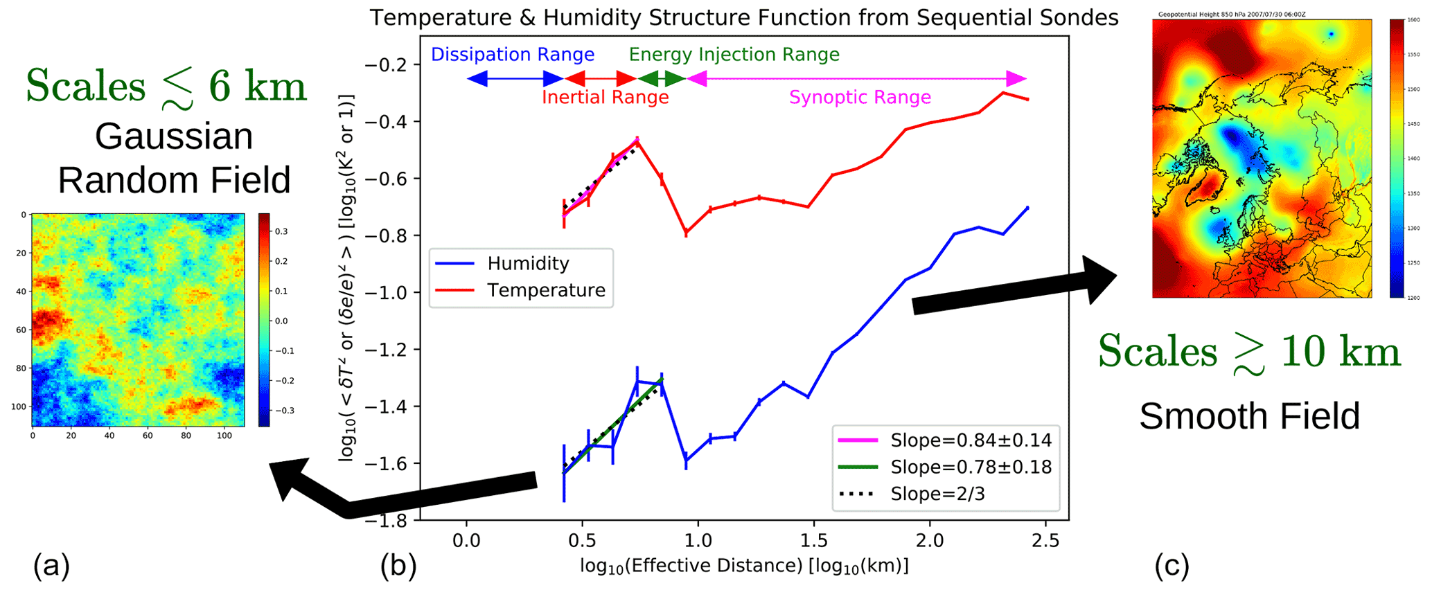
Figure 1Panel (b) shows an observational temperature and water vapor structure function obtained from horizontal comparisons of temperature and water vapor concentrations (for more details see text or Calbet et al., 2018). Panel (a) shows a mathematically synthetically generated GRF representative of small spatial scales, while panel (c) shows a smoothly varying NWP field representative of larger spatial scales (analysis of geopotential height at 850 hPa from 30 July 2007 at 06:00Z).
A key concept in Kolmogorov's theory of turbulence is that of the structure function. This shows how the average of the squared difference of a fluid parameter between two spatially separated points behaves as a function of their distance. Usually, a log–log plot is used to make this representation. This is illustrated in the central panel of Fig. 1, where the structure function for temperature and water vapor at different scales is shown. The structure function has been obtained by horizontally comparing radiosonde measurements of temperature or water vapor concentrations layer by layer. For more details on the technique see Sect. 3.1 or consult Calbet et al. (2018) for a broader discussion. Note that the temperature and water vapor structure functions have different units in the vertical axis. While water vapor differences are relative, hence with no units, temperature differences are shown in Kelvin. This plot shows the usual behavior seen in fluids in the laboratory (e.g., Frisch, 1995; Noullez et al., 1997). Namely, at small scales, known as the inertial range, the log of the variance of the difference grows linearly with the log of the distance following a two-thirds slope. This is what is known as the two-thirds law (Frisch, 1995). At longer scales, the average of the differences squared diminishes with distance. This is the energy injection range shown in Fig. 1. At even longer scales, this average increases with a slope steeper than the one in the inertial range. This is denominated the “synoptic range” in this paper. Here synoptic range is understood in a very relaxed sense ranging from a few tens to several thousand kilometers.
Apart from the energy injection range, which, as we shall see later, is difficult to see with other instrumentation due to its narrow range, the conclusion that can be drawn from Fig. 1 is that the atmosphere can be divided into two different ranges and behaviors. Above approximately 10 km on average we have what is called here the synoptic range. The atmospheric parameters can be regarded as a more or less smooth field, and this is what is usually reproduced well by global NWP models. Below 6 km on average we have the inertial range, where the structure function follows the two-thirds law. In this range the water vapor field is extremely inhomogeneous and resembles a GRF.
It should also be noted that these considerations apply when averaging a big sample of measurements. In practice, when taking a smaller sample, the structure function will vary significantly from one region to another. One of such deviations from the average structure function is the location in the vertical axis of the inertial range. If the data that fit the two-thirds law are high along this axis, it would indicate a high turbulence or a high-horizontal-concentration variability regime. If the data are placed in a lower place along the ordinate axis, they would nominally indicate a lower turbulence or concentration variability. The exact position where these points lie in the structure function graph will depend on the degree of turbulence of the region being analyzed. Another deviation from the average structure function is the frontier between the inertial and the synoptic range, which can, as we shall see later, vary significantly from one region to another. But, for the atmosphere on average this frontier lies around 6 to 10 km in the horizontal.
Kolmogorov's theory also implies that in the inertial range the parameter under study follows a GRF on average. To have a feeling of how a GRF looks, the far left image in Fig. 1 shows a synthetically generated one, which is explained in more detail below. This is the behavior we can expect from the parameter field at small scales, which can be useful in obtaining further conclusions from the measurements.
2.2 Gaussian random fields (GRFs)
In this paper the only parameter we will focus on is one scalar field, namely the atmospheric water vapor concentration. This study could easily be extended to more parameters, like temperature. A field is defined by
where x is the position in space which constitutes the two horizontal dimensions. The third vertical dimension will be dealt with in the following section.
A random field is one in which the value of the parameter is random and follows a certain probability distribution. In the case of Gaussian random fields (e.g., Rue and Held, 2005), if we have the value of a field, f, in position x1 and another one in position x2, these random values will follow a multivariate Gaussian distribution such that the expected value of the field is
and their covariance is
where the symbols 〈〉 denote the expected values of the parameters enclosed within them. It is also usually assumed, as will be done here, that the field is stationary, meaning the mean is constant,
Another condition that is often used is that it is also homogeneous and isotropic, meaning that the covariance is only a function of the Euclidean distance,
The structure function is defined as the relation between the expected value of the squared field difference between two points versus their distance. If it is further assumed that the fluid is in the inertial range where Kolmogorov's theory applies (Frisch, 1995), then defining the distance between two points as
the structure function, defined as S(r), will follow the two-thirds law:
Note that K is a measure of the variability of the field or, equivalently, provides a measure of where the curve is placed in the vertical axis of the structure function plot.
The notation of the covariance can now also be simplified to
The relationship between the structure function and the covariance will be needed in a later stage. Some simple algebra shows that
which implies that the structure function has similar algebraic behavior as the covariances.
In the real atmosphere, all this is, of course, a simplification. Nevertheless, we will show that this approximation holds relatively well for small scales of observed water vapor concentrations. In summary, a Gaussian random field (GRF) will be understood in this paper as a random field satisfying Eqs. (2), (3), (4) and (7).
2.3 Consideration of the vertical dimension
In this subsection very brief mention will be made of how the vertical dimension can be dealt with. These considerations are particularly important for satellite remote sensing in the thermal infrared or microwave spectral region.
Adding the vertical dimension to the two horizontal ones would complete the study in the three-dimensional space. In meteorology and satellite remote sensing it is convenient to divide the atmosphere into vertical layers. Satellites, in particular, can be considered instruments observing the atmosphere divided into several layers of finite thickness. For example, in the thermal infrared, to a very rough first approximation, for any one spectral channel the measured satellite radiance can be considered an average emittance over several layers. Therefore, the particulars of the structure function observed by the satellite will depend on the vertical correlation between these layers. If the layers have completely independent statistical properties, then the covariances of each layer can be averaged independently to give the combined covariance. This would constitute the typical covariance diminishing factor of the average of a random variable. If, on the other hand, the layers have a perfect vertical correlation, then the covariances of all the layers combined will be equal to the covariance of just one layer. In both cases, the structure function would follow behavior similar to the covariance because of Eq. (9).
In summary, if the vertical layers are statistically independent, the satellite-observed structure function will have a much lower K value (or covariance) than each individual layer. The physical reason behind this is that the effect averages out as the different layers contribute in completely independent ways. If, on the other hand, the layers have a perfect vertical correlation, then the structure function of the combined layers will be the same as the one for an individual layer. This can be conceptually idealized as if we had identical values for all layers. In other words, for the GRFs to be visible from satellite observations some form of vertical correlation between atmospheric layers is needed to have an observable effect. This will come naturally in some specific meteorological cases such as the presence of water vapor rolls which do show a high vertical correlation (Carbajal Henken et al., 2015).
In this paper, one NWP model (ECMWF) and data from several satellite and radiosonde instruments have been used. These datasets are detailed in the following subsections.
3.1 Radiosonde data
The radiosonde measurement data are from the EUMETSAT EPS/MetOp campaigns made in 2007 and 2008 at Lindenberg (Germany) and Sodankylä (Finland) observatories (Calbet et al., 2011). In these campaigns, two consecutive radiosondes were launched from the same site separated by about 50 min in time. These types of measurements are usually referred to as sequential sondes. The instrument payloads analyzed here are the conventional RS92 radiosondes. The data have been processed by GRUAN (Dirksen et al., 2014), which, among other advantages, greatly removes the humidity measurement dry biases usually present in RS92 measurements at the high troposphere (Miloshevich et al., 2009).
Sonde measurements sample the atmosphere every second as the radiosonde ascends in the air. This effectively means measuring the troposphere in layers around 0.6 to 0.1 hPa thick in the pressure levels used in this study. They range from 950 to 200 hPa, respectively. The humidity measurements from the first radiosonde of the sequential sonde pair is vertically interpolated to the vertical pressure grid of the second sonde. By doing this, both water vapor measurements from each pair of sequential sondes can be compared directly. To calculate the structure function, the normalized differences between water vapor partial pressure measurements from each radiosonde at the same pressure level are calculated. All water vapor units are converted using the Hyland and Wexler (Hyland and Wexler, 1983) saturation formula. If e1 and e2 are the partial water vapor pressure for the first and second sonde, respectively, then the normalized difference is calculated with
Note that this quantity has no units.
For temperature, the temperature difference is directly calculated,
where T1 and T2 are the temperatures of the first and second radiosonde, respectively. Its corresponding unit is Kelvin. To these differences, an effective distance is assigned. This effective distance is the real spatial distance between sequential sondes plus the time difference multiplied by the wind speed measured by the radiosondes at that level. The average of the square of this normalized water vapor concentration or temperature difference is then calculated for different effective distance bins. In order to achieve a significant sample size, results from all sample pairs and for all radiosonde pressure levels between 950 and 200 hPa have been combined. The resulting total number of data pairs, coming from the 625 sequential sonde pairs, is 658 217. From these calculations, the structure function for both temperature and water vapor can be plotted. This is shown in Fig. 1. For more details on this see Calbet et al. (2018).
3.2 SEVIRI on board MSG
The Spinning Enhanced Visible Infrared Imager (SEVIRI) is an imager instrument on board the Meteosat Third Generation (MSG) geostationary satellite (Schmetz et al., 2002). SEVIRI is a 50 cm diameter aperture, line-by-line scanning radiometer. It provides image data in four visible and near-infrared channels as well as eight infrared channels. The only channel used in this paper is the one centered at 6.25 µm with a spectral interval in which 99 % of the energy is detected between 5.35 and 7.15 µm and a NEΔT=0.75 K at 250 K. Its spatial resolution (sampling distance) is 3 km at the sub-satellite point. The SEVIRI instrument measures the complete observable disk from geostationary orbit with a repeat cycle of 15 min. It yields an image for the 6.25 µm channel of 3712×3712 pixels covering the complete disk for each repeat cycle. The images used are radiometrically calibrated and geolocated. They have been obtained via the EUMETSAT archive in High Rate Information Transmission (HRIT) format (Level 1.5).
The SEVIRI image date and time for the determination of the structure function have been selected randomly and correspond to 20 August 2019 at 10:00Z. The corresponding “air-mass RGB” image can be seen in Fig. 2. To avoid effects of a high satellite zenith angle in the radiative transfer, a region centered in the sub-satellite point has been selected. The region is a square of 1000×1000 pixels centered at nadir (roughly an area of 3000×3000 km2). It is highlighted in Fig. 2 as a red square.
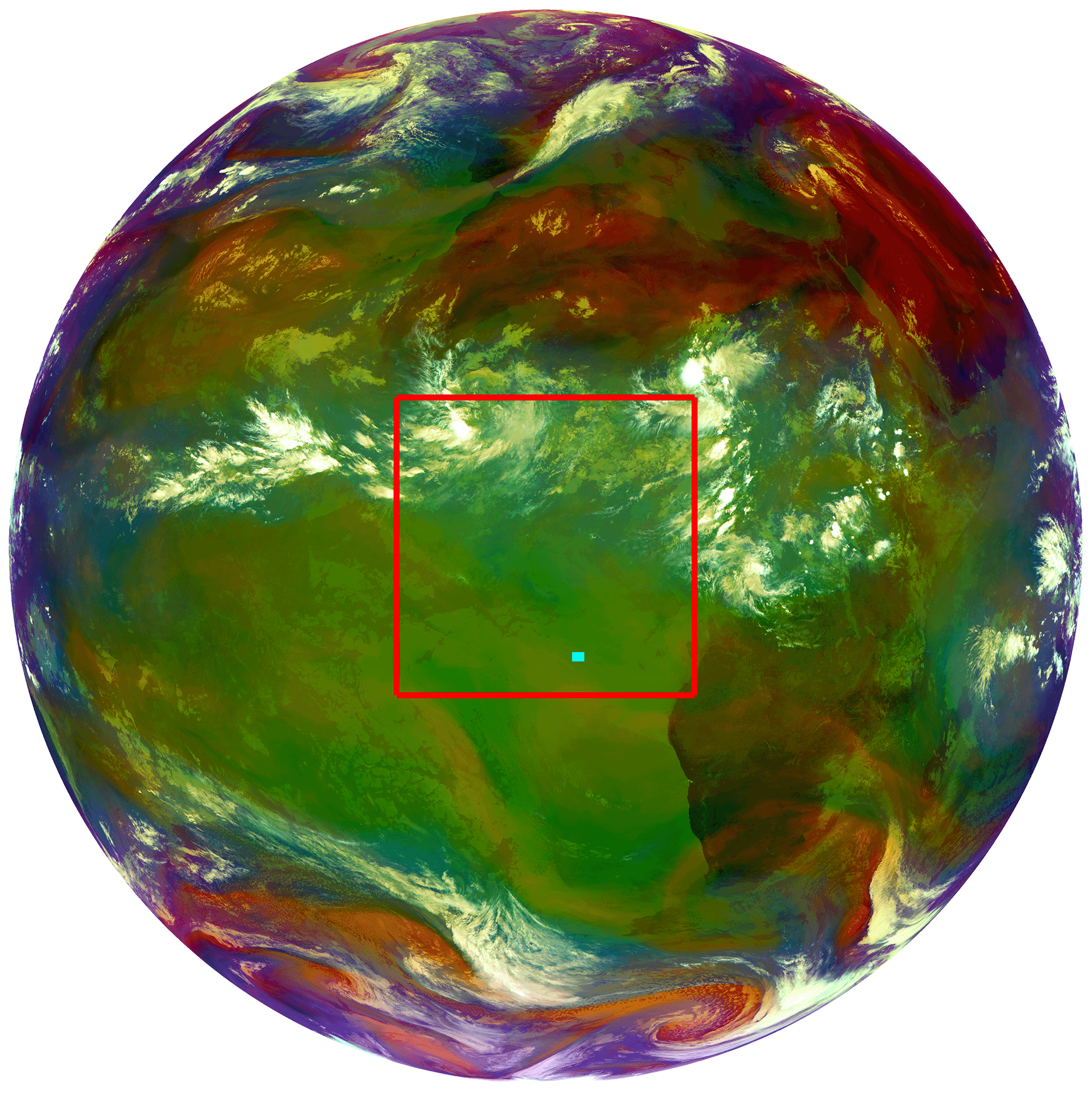
Figure 2SEVIRI/MSG “air-mass RGB” image of the date and time selected (20 August 2019 at 10:00Z). Highlighted in red is the analyzed region. In cyan, the location of the ECMWF profile selected for RTM calculations is shown.
The 6.25 µm channel is centered, from the spectroscopic point of view, in the highly absorptive portion of the water vapor band. It is therefore a channel that mainly detects water vapor in the high troposphere. Because of this, it is classified as a “water vapor” channel. It is almost completely insensitive to surface effects such as skin temperature or surface emissivities, simplifying its radiative transfer modeling. For all these reasons it is used to detect water vapor in the high troposphere, a magnitude that will be denoted as high-level column water vapor (HLWV) in this paper. The HLWV will be the integral over a column of the water vapor content between 500 and 0 hPa and will have units of millimeters of water (denoted as mm).
The structure function could be determined directly from the measured radiances, but these do not constitute an atmospheric parameter. It is therefore best to convert these radiances into a measurement of water vapor such as the HLWV defined above. A thorough retrieval, such as optimal estimation, within each Meteosat pixel could be derived. But, since the structure function is robust to any such estimations and it seems more illustrative for the reader to use a simple regression, only a first-order approximation of the HLWV will be performed. To estimate the HLWV from the 6.25 µm channel radiances we start by using an atmospheric profile representing roughly all other atmospheric profiles in the selected region. The profile has been chosen to be inside the selected region and sufficiently far away from any high-level clouds. Its location is shown as a cyan dot in Fig. 2. The temperature and water vapor values of the profile are obtained from an NWP forecast model of the region. In particular, it is an ECMWF forecast from an analysis on 20 August 2019 at 00:00Z and a forecast step of 10 h. The top-of-atmosphere radiances are calculated for this profile using the RTTOV radiative transfer model (Saunders et al., 2018). The water vapor content of this profile is perturbed at all levels and with varying satellite zenith angles such that the radiance dependency versus the HLWV is obtained. Once this synthetic dataset is calculated, the resulting HLWV is regressed to the radiance and satellite zenith angle, obtaining the following fit
where R6.25 µm is the measured radiance in mW m−2 sr−1 cm, θ is the satellite zenith angle and the output units for HLWV are millimeters (mm).
The RTM requires that only scenes unaffected by clouds are analyzed. Since the 6.25 µm channel mainly sees the upper troposphere, scenes with any mid-level or high clouds need to be excluded. To do this, the Nowcasting Satellite Application Facility (NWC SAF) software package (NWCSAF, 2018) for geostationary (GEO) satellite data is used. The NWC SAF provides a set of software packages to derive meteorological products from satellite data. Among all the satellite products available from the NWC SAF, the cloud type (CT) product is the one needed here. It is generated for this particular region, providing cloud types as a categorical variable. Only pixels with scenes that are clear or with very low-level clouds are selected for the analysis.
3.3 OLCI on board Copernicus Sentinel-3
The Ocean and Land Color Instrument (OLCI) is a push-broom imaging spectrometer that measures solar radiation reflected by the Earth. OLCI is on board the polar sun-synchronous Sentinel-3 Earth observation satellite series dedicated to ocean and land observation (Donlon et al., 2012). OLCI measures in a swath width of 1270 km with a ground spatial resolution of 300 m in 21 spectral bands between 400 and 1020 nm. Their radiometric accuracy is 0.1 %.
From this instrument a retrieval of total column water vapor (TCWV) can be performed. The method used in this paper is based on the Copernicus Sentinel-3 OLCI Water Vapor (COWa) product. It uses an optimal estimation method to retrieve TCWV from the Oa17, Oa18, Oa19 and Oa20 OLCI bands. Because of this, it provides both a measurement of the TCWV and its uncertainty. The properties of the OLCI channels allow for accurate determination of the TCWV over land in clear-sky scenes. The TCWV estimation over ocean is far more uncertain and is not used in this paper. The method is fully described in Preusker et al. (2021).
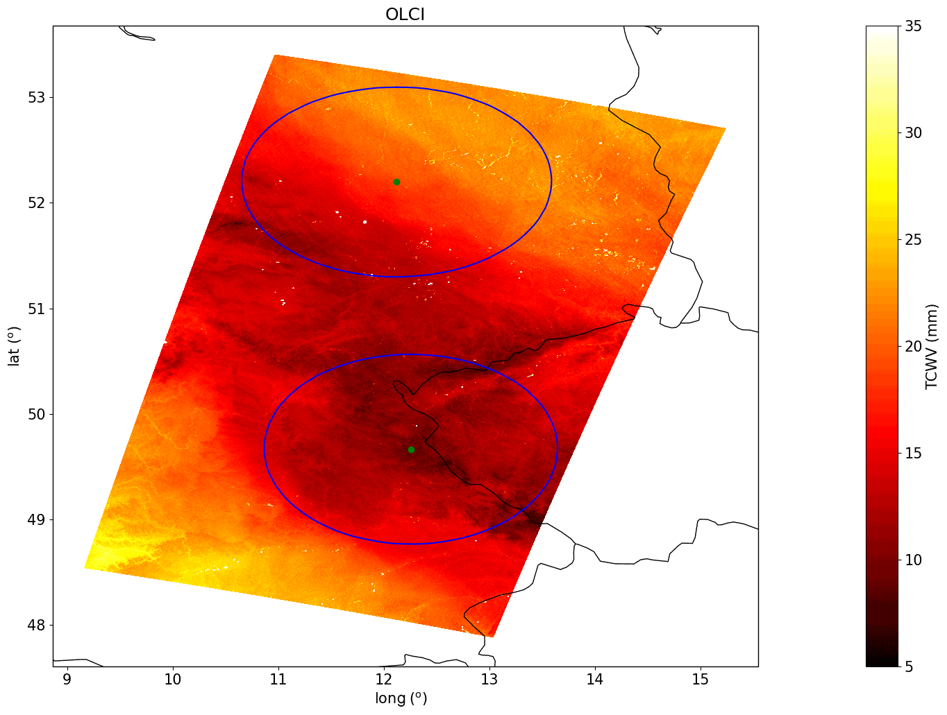
An image on 31 August 2016 at 09:45Z covering southeastern Germany and the western Czech Republic has been selected. This region is located over land and consists mostly of clear-sky pixels, making it an ideal candidate for the accurate measurement of TCWV with the OLCI. TCWV for this field is represented in Fig. 3. Cloudy classified pixels are plotted in white. The high horizontal variability of water vapor can be clearly spotted in this image as has been recognized before (Carbajal Henken et al., 2015). As explained in Preusker et al. (2021), each pixel has its own precise value of uncertainty; however, to have a mental picture, we can keep in mind that the uncertainties of all pixels in this region are around 0.33 mm.
3.4 ECMWF NWP model
A comparison of the measured structure functions and small-scale horizontal variability with other sources can be instructive. For this reason, the same region as the one selected for OLCI is also selected for an NWP model. It should ideally be a high-resolution regional model. Since such a model was not available at the time of writing of this paper, the NWP model used here is the operational global ECMWF one. The data are retrieved from ECMWF's archive and obtained with a regular latitude–longitude grid of 0.125∘ × 0.125∘. Only the TCWV parameter is obtained from the model, which is a forecast predicted from an analysis on 31 August 2016 at 00:00Z with a step of 10 h; this implies a valid time of 10:00Z on that same day. The field is plotted in Fig. 4. The blue line indicates the contour of the corresponding OLCI observation from Fig. 3. A quick visual comparison of OLCI's and ECMWF's TCWV fields (Figs. 3 and 4) shows that they both share similar structures. The ECMWF field shows a lower spatial resolution and smaller contrast, indicating a lower TCWV range with respect to OLCI.
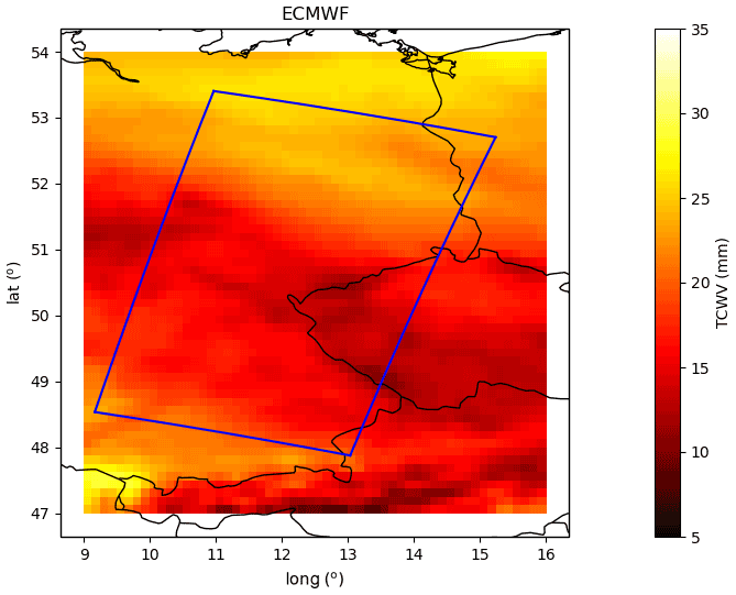
Figure 4ECMWF forecast TCWV field from 31 August 2016 valid at 10:00Z (10 h step from an analysis at 00:00Z). The contour of the OLCI observation from Fig. 3 is shown in blue.
In this section the methods applied to the data are discussed. In a first subsection, the way to calculate the structure function from the data is explained. Two different types of structure functions are calculated. The first one is denominated “pixel-centered structure function”. It is a structure function that is calculated on each and every pixel of the image. The second one is an “average structure function”, and, as the name indicates, it is a structure function calculated by averaging many pixel-centered structure functions.
In a second subsection, the calculations to derive the typical mathematical properties of GRFs are explained. Also, a histogram is obtained from the measurements, which should follow a Gaussian distribution. Several synthetic GRFs are generated, which are later compared to the measurements.
4.1 Water vapor structure function
The water vapor structure function is calculated from the data in two different ways. One of them is centered in a particular pixel of the field or image, which will be called the pixel-centered structure function. The second one is an average over the whole satellite image or NWP field, which will be denoted as the average structure function. The way to calculate them is described below.
4.1.1 Pixel-centered structure function
The goal is to have a structure function centered on each and every pixel within the satellite image or NWP field. Depending on the source of the data, the water vapor structure function is calculated for different parameters: TCWV for OLCI and ECMWF, HLWV for MSG. Note that for radiosondes (Fig. 1) the partial water vapor pressure was used. To simplify the notation, any of these water vapor parameters will be denoted by the variable w. The pixel where the structure function is calculated will be denoted as the “central pixel” regardless of its location within the image or field. The very first step is to divide the total distance range from the minimum observable by the instrument to a maximum of 100 km into several discrete bins. Then, the relative difference between the parameter in the central pixel and all the surrounding ones up to a distance of 100 km is calculated. Similarly to what was done for sondes in Eq. (10), the relative difference is defined as the difference of the parameter divided by the average. So, if w0 is the water vapor parameter located in the central pixel and w1 is the water vapor parameter of a pixel at a certain distance from the central one, then the relative difference is defined as
Note that in the case of satellite measurements or NWP fields used in this paper, the measure of water vapor (w) is a columnar amount (TCWV or HLWV), while for the sondes it was a point measurement of partial pressure of water vapor (e) at a certain pressure.
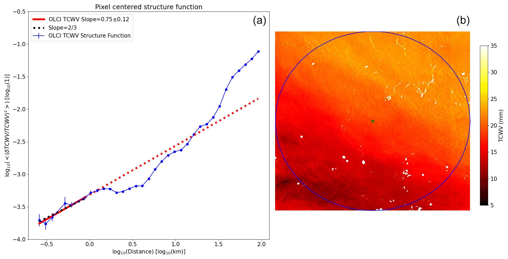
Figure 5Pixel-centered structure function for the OLCI COWa TCWV shown in panel (a) together with its uncertainty in the vertical axis (blue curve), a linear fit of the points below 100 km (red curve) and a two-thirds slope line (black dots). The structure function covers the area inside the blue circle shown in the right TCWV image (b), which has a radius of 100 km and is centered in the green dot. This region is a zoom of the top left region highlighted in blue from Fig. 3. Cloudy classified pixels are plotted in white.
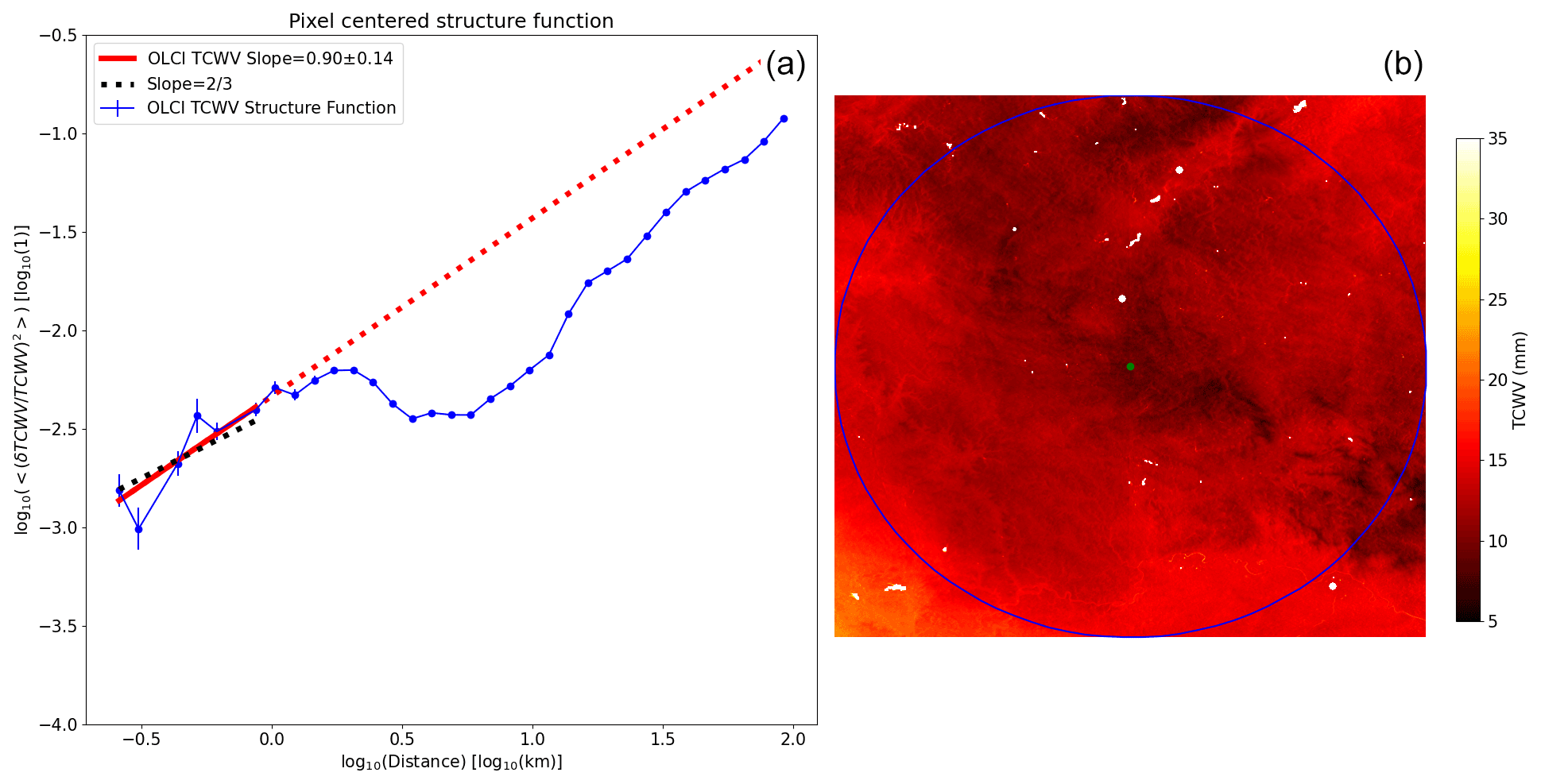
Figure 6Pixel-centered structure function for the OLCI COWa TCWV shown in panel (a) together with its uncertainty in the vertical axis (blue curve), a linear fit of the points below 100 km (red curve) and a two-thirds slope line (black dots). The structure function covers the area inside the blue circle shown in the right TCWV image (b), which has a radius of 100 km and is centered in the green dot. This region is a zoom of the bottom right region highlighted in blue from Fig. 3. Cloudy classified pixels are plotted in white.
After this, the distance between these two points is calculated. The square of the relative difference is calculated and its value is accumulated into its corresponding distance bin. A record of the number of occurrences in each bin is kept. To achieve relevant statistics, especially for the short distance ranges, the number of cases needs to be increased. This is done by shifting the pixel where the origin of distances is located around a 5×5 pixel square surrounding the central pixel. In other words, the exact same calculation is repeated within a 5×5 pixel square surrounding the central pixel. Once all the points are processed, the average is calculated by dividing the accumulation by the number of occurrences in each distance bin. The uncertainty of this average is also estimated statistically. In the end, the average of the relative difference squared, , together with its uncertainty, as a function of distance is obtained. To obtain the structure function, the logarithm in base 10 of these two quantities can be plotted. Examples of pixel-centered structure functions can be seen in Figs. 5 and 6. Note the different y intercepts when comparing these figures due to the different inhomogeneities or turbulence intensities. The white regions in these figures correspond to pixels where the potential presence of clouds has been detected and have therefore been masked out. These figures have been generated for all the pixels on the complete OLCI field, all showing similar results and also a good fit to the two-thirds law.
4.1.2 Average structure function
To reduce the uncertainties in the structure function or to have a global picture of it, it is convenient to obtain an average of all the pixel-centered structure functions of a given instrument. This is done in three steps.
-
The first step is to bring all cases to the same vertical axis in the structure function. This is achieved by averaging the structure value, , for all distances smaller than a threshold. This threshold distance is the maximum distance at which the structure function still approximately retains the two-thirds slope for all the pixel-centered structure functions of a given instrument. Defining this threshold as rlim, this average, ai, can be defined in mathematical form as
where the sub-index i labels a particular central pixel in the pixel-centered structure function and emphasizes that there will be the same number of ai as pixels in the image or field. ri denotes the distance of any other pixel to the central one. The average of this parameter, denoted by a, will also be important:
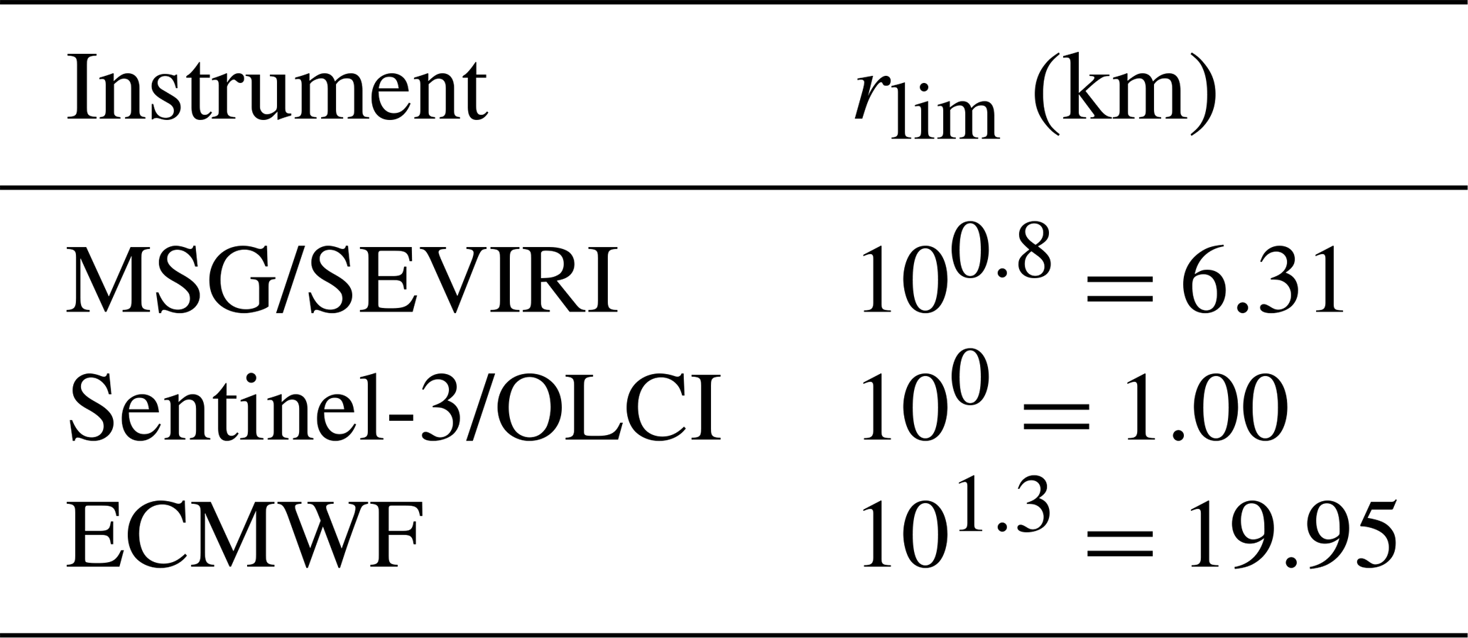
Because of their different spatial resolutions, the values of rlim will depend on the instrument or model used. Table 1 summarizes the values used for different instruments or models. These values have been derived by empirically verifying that below this distance the pixel-centered structure function approximately retains the two-thirds slope for these pixels. The NWP model data (ECMWF) are exceptional because they lack the very small scales, and the rlim value in Table 1 is one for which a meaningful average can be obtained.
-
All components of the structure function are normalized by the ai factor, taking into account the logarithm, such that they are all brought to the same level,
-
These rescaled structure function components are now averaged and brought back to the average level,
-
Finally, the logarithm of this quantity is taken to have the final value for the average structure function,
Examples of various average structure functions are shown in Fig. 7.
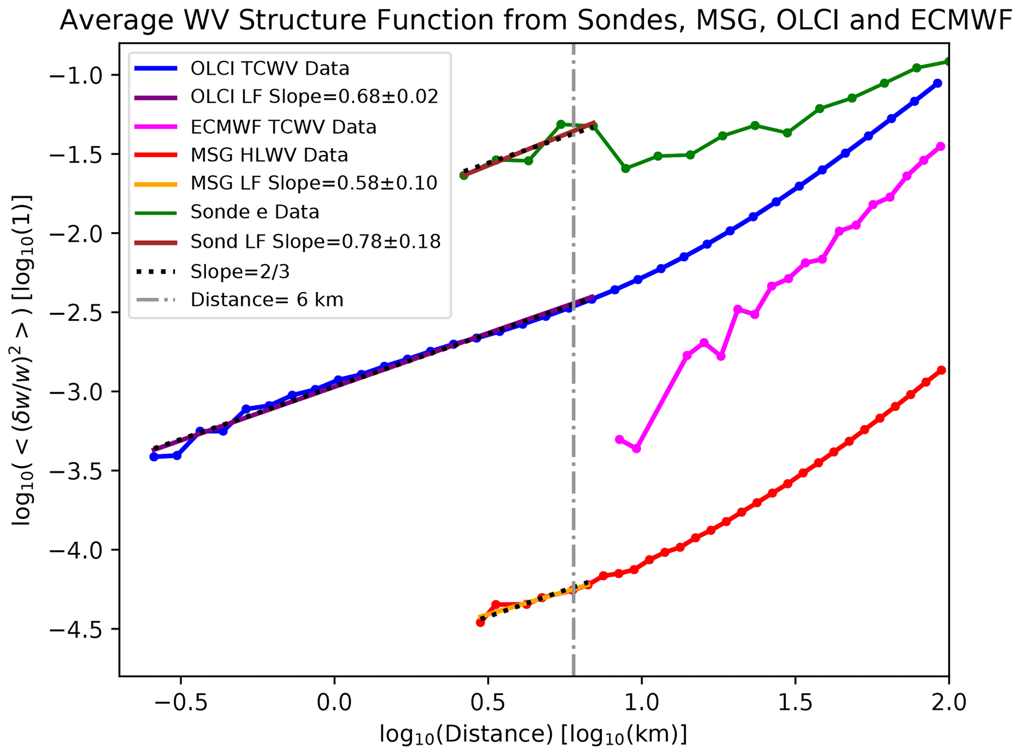
Figure 7Average structure functions for MSG/SEVIRI (red), Sentinel-3/OLCI (blue) and the ECMWF forecast (magenta). Also plotted is the plain structure function from radiosondes (green). Linear fits below ∼ 6 km are also shown (orange, purple and brown) together with two-thirds slope lines (black dots). The distance of 6 km is highlighted as a vertical dash-dotted gray line.
4.2 Gaussian random fields
To demonstrate that water vapor structures at small scales do resemble GRFs we must first verify that measurements on an individual pixel do follow a Gaussian distribution by looking at its histogram. As a second step, water vapor measurements must visually resemble a GRF. For this, two synthetically generated GRFs have been created which can be compared to a spatial zoom into an OLCI TCWV measurement region. How these plots have been generated is described below.
4.2.1 Gaussian histogram
A square of 60×60 pixels (roughly 18×18 km) is selected from the OLCI TCWV measurements. The TCWV values of all the pixels in this square are subtracted from the average TCWV. This is repeated for all other similar square areas over the complete OLCI measurement region without any overlap between the squares. All these TCWV differences, δTCWV, are collected together to generate a normalized histogram. This is shown in Fig. 8. Also plotted is an overlaid Gaussian function with standard deviation equal to the one obtained from the data (0.899 mm).
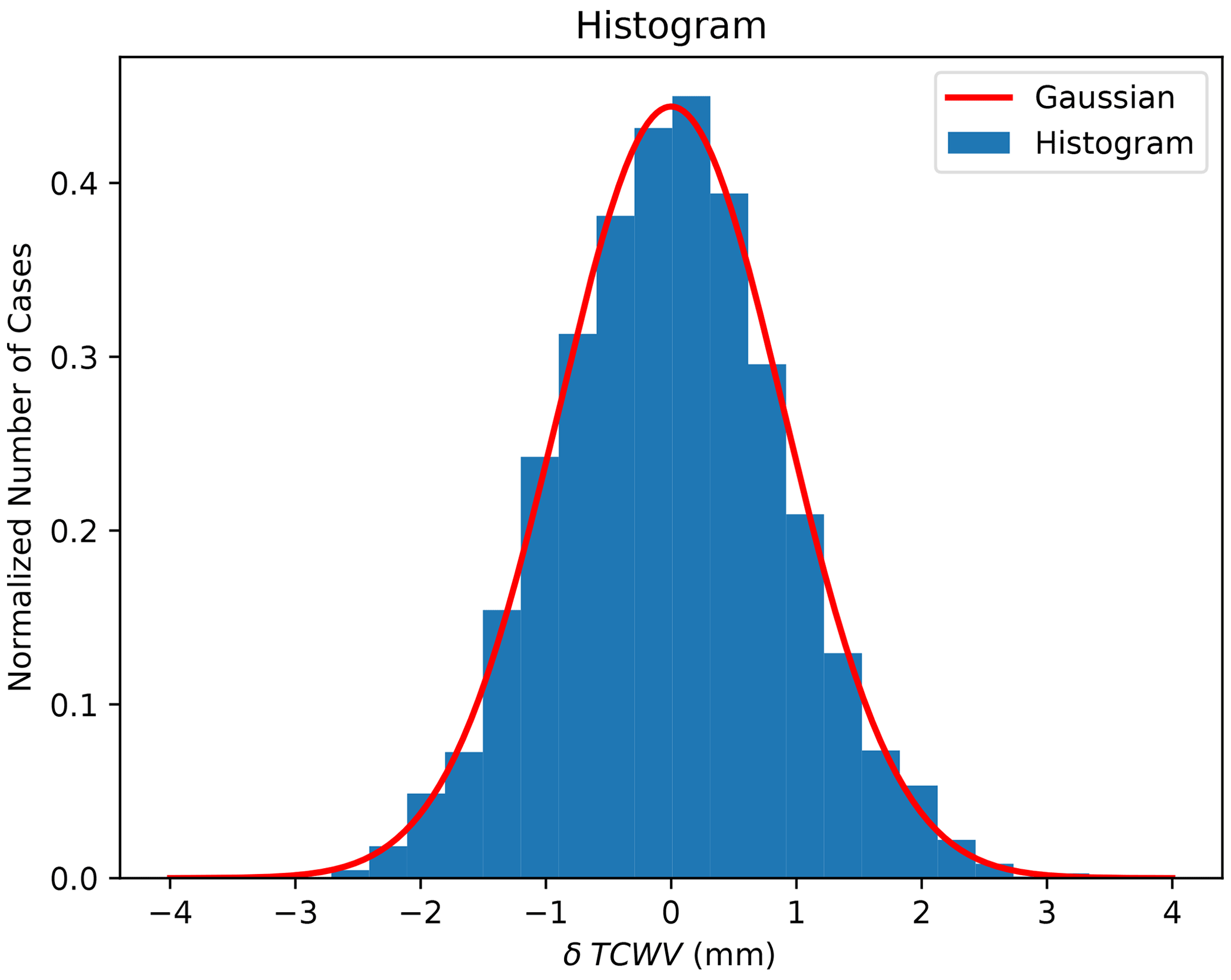
Figure 8Normalized histogram of TCWV differences calculated in boxes within the complete OLCI measurement region (blue) and a Gaussian function with a standard deviation obtained from the data (red).
4.2.2 Synthetic GRFs
To produce a representation of the product noise or uncertainty, a GRF with its standard deviation equal to the average OLCI COWa TCWV uncertainty (around 0.33 mm) and also with no spatial correlation (C(r)=0) is plotted. This is represented in the left image of Fig. 9.
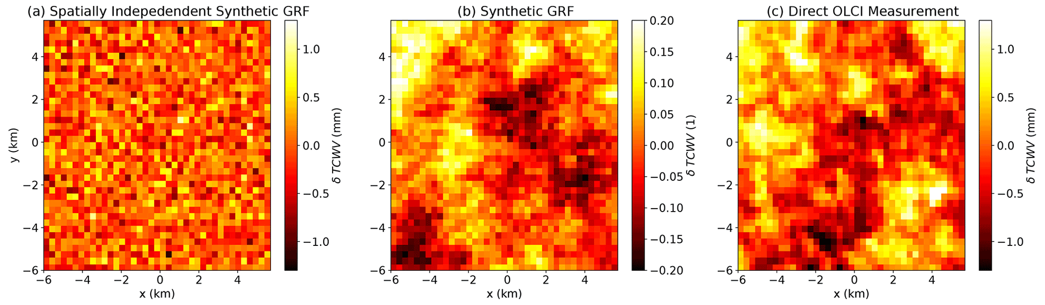
Figure 9Spatially independent (C(r)=0) Gaussian field with standard deviation equal to the OLCI COWa TCWV estimated uncertainty (a), Gaussian random field following the two-thirds law (b) and OLCI COWa TCWV difference close-up image from Fig. 3 centered in (long, lat) = (12.2344∘, 49.6135∘) (c).
To generate a synthetic GRF which follows the two-thirds law, an algorithm following the isotropic spectral method (Paludo et al., 2015) has been selected. The result can be seen in the central image of Fig. 9.
4.2.3 Measured OLCI TCWV fields
To appreciate the small-scale features of the OLCI COWa TCWV fields, a zoom has been performed in a randomly selected region centered on (long, lat) = (12.2344∘, 49.6135∘) and covering an area of about 6×6 km2. This is shown in the right image of Fig. 9. Any other region selected would show the same structure.
In this section, the results are shown. First, the structure functions will be discussed, and, in a later section, qualitative and quantitative views of the GRFs will be shown.
5.1 Structure functions
The average structure functions for several meteorological satellites and the ECMWF NWP model are shown in Fig. 7. Also shown is the plain structure function from radiosondes (green curve) obtained from Calbet et al. (2018). Although they all constitute structure functions for relative differences of water vapor, in these plots we emphasize that different water vapor concentrations, pressure levels, spatial regions and valid times have been used. The radiosonde structure function is calculated from the partial pressure of water vapor and spans pressure levels from 950 to 200 hPa. The MSG structure function has been derived from the column water vapor from 500 to 0 hPa, which is referred to as HLWV in this paper. The OLCI and ECMWF structure functions are taken for very similar regions and valid times and also using the same TCWV water vapor parameter, so they should be very comparable.
Figure 7 clearly demonstrates how all structure functions quite precisely follow a two-thirds law for spatial scales smaller than approximately 6 km. This is highlighted by the linear fit shown in this same figure and labeled as LF. The slope of the fitted linear regression is also shown in the inset together with its uncertainty. A linear fit with an exact two-thirds slope is also shown as the dotted black line for comparison. All linear fit slopes show a two-thirds value within their uncertainty range.
Another distinct feature of this figure is the wide range of horizontal variability of water vapor, i.e., the different displacement of the curves in the vertical axis. The radiosonde data measure in very thin layers of at most 0.6 hPa in depth. All the other instruments measure in extremely thick layers or even the complete atmospheric column. This implies that the diminishing of the variance (smaller K values) as the vertical integration range increases might play a significant role here (see Sect. 2.3).
Even though they are indeed measuring the same parameter at the same location in space and time, the contrast between the OLCI and ECMWF NWP curve is significant. Since the ECMWF NWP is a global model with a coarser resolution, it lacks the information at scales smaller than 6 km. Also, the horizontal variability of the ECMWF model is significantly smaller than the one from OLCI. This can also be verified visually by comparing the direct products from Figs. 3 and 4. The reason for this could be a low representativity of the ECMWF NWP model, or it could be caused by the NWP model trying to average the water vapor over the small scales due to its horizontal scale and the way it handles the water vapor. The consequence of this is clear: a global NWP model might have a lower horizontal variability than other higher-resolution measurements. In any case, the final reason for this is unknown and further investigation on this subject is required.
Finally, a feature that also stands out is the presence of a small region in which the horizontal variability decreases with increasing distance, which is present in the OLCI pixel-centered structure functions (Figs. 5 and 6) and the sonde structure function (Fig. 1, labeled as “energy injection range”, or the green curve in Fig. 7). This is clearly absent for the average structure functions from MSG, OLCI and ECMWF in Fig. 7.
The pixel-centered structure functions obtained from OLCI, two of which are shown in Figs. 5 and 6, are also interesting. It can be verified that the horizontal variability also changes significantly from one region to another, as seen by the vertical location of the structure functions shown in the left plots of these figures. This horizontal variability difference spans almost an order of magnitude between these two regions. The inertial range, in which the structure function follows a two-thirds law, also has different sizes depending on the region. The region in Fig. 6 has a slightly smaller inertial range size (∼ 1.5 km) than the one in Fig. 5 (∼ 1.8 km), and both of them are well below the average value of 6 km. In these pixel-centered structure functions, the inertial range does not closely follow a two-thirds law as opposed to the averaged structure functions seen before. In particular, Fig. 6 shows a fairly “noisy” structure function in the inertial range and its slope is quite far away (0.90±0.14) from the ideal two-thirds value. Both of them show a range in which the horizontal variability decreases with increasing distance, the energy injection range mentioned above.
5.2 Gaussian random fields
The first property for a random field to be Gaussian is that individual pixels must follow a normal distribution. This is verified in the histogram plotted in Fig. 8, which closely follows this behavior.
To show that the OLCI TCWV does indeed behave like a GRF, several different panels are represented in Fig. 9. In the right panel of Fig. 9 the actual measured TCWV difference field has been plotted. More specifically, the difference with respect to the average of the field is shown, which is labeled as δTCWV in the figure. This precise region is a zoom of the image shown in Fig. 3 centered at (long, lat) = (12.2344∘, 49.6135∘). Although a particular region of the OLCI measurements has been selected for the right image of Fig. 9, any other region within the complete field (Fig. 3) shares the same general aspect at these small scales.
In the left panel, a somehow especially restricted GRF has been generated. Its particularity is that it has no spatial correlation (C(r)=0) and the standard deviation of its normal distribution is set to σ=0.33 mm. This value is approximately equal to the uncertainty of all the OLCI COWa TCWV pixel retrievals used throughout this paper. This is exactly how the measurements would look if only “retrieval noise” were present. The measured TCWV (right panel) shows very different behavior. The measurements show a spatial correlation not present at all in this synthetic field, and also the variability is much higher than the simulated counterpart.
The measured TCWV can be compared with a synthetically generated GRF that does follow a spatial correlation under the two-thirds law. This is shown in the central panel of Fig. 9. The general aspect is remarkably identical to the measurement. This constitutes further proof that water vapor concentration in the atmosphere does indeed resemble a GRF at small scales.
The average structure function quite accurately follows a two-thirds law at small scales for several instruments (Fig. 7). This implies that the atmosphere, on average and at these scales, follows Kolmogorov's theory of turbulence. As a consequence, water vapor fields can be approximated as Gaussian random fields (GRFs) at these scales. Given the caveat that this is a limited study (not all seasons or climate zones are covered), the fact that similar results are obtained from measurements at different layers and from various instruments seems to prove that this is a universal property which applies at all these ranges.
To confirm this, the histogram of individual pixels is shown to follow a Gaussian distribution (Fig. 8). Furthermore, the direct high-resolution measurements of water vapor in the atmosphere (right panel of Fig. 9) show clear similarities with synthetically generated GRFs with similar spatial properties (central panel of Fig.9).
These assumptions can be applied only to scales below approximately 6 km on average. They do not apply at scales greater than this value, since the structure function deviates from the two-thirds law (Fig. 7) and the water vapor fields leave the GRF variability and start showing a “synoptic” structure (Figs. 3 and 4). This typical scale approximately coincides with other similar studies made with GPS phase difference observations (Kermarrec and Schön, 2020), which estimate an outer scale of turbulence of around 4 km, or with modeled atmospheric turbulence simulations, which show an outer scale length for potential temperature of about 10 km (Fig. 1 from Tung and Orlando, 2003).
As a consequence of these results, the water vapor concentration in the atmosphere is inherently turbulent and chaotic at these small scales. There will always be a random component which will be impossible to measure on a full spatial scale in general and, in particular, that of a typical satellite infrared sounder instrument with a footprint of 15 km. Water vapor near the surface is also a critical parameter for the triggering of convection. This means that nowcasting will always have an inherently stochastic component associated with it. Because of this, it is highly likely that the best approach to making forecasts for nowcasting would be to have a probabilistic method.
Global NWP models do not seem to be able to accurately reproduce the intensity of the horizontal variability of water vapor at small scales (Fig. 7). They also do not yet have the spatial resolution to resolve them. It is therefore imperative to use other methods to estimate this small-scale horizontal variability of water vapor. Measurements or NWP models with a high spatial resolution could be a practical solution if these kinds of features are needed.
All these results can be of practical importance to estimate the horizontal variability of water vapor within a region. It can also be applied in making several neighboring measurements consistent, since the random differences between two measurements can be estimated. The uncertainty usually present in the estimation of the atmospheric processes involved in convection could potentially also benefit from the proper characterization of water vapor horizontal variability.
The code is simple enough to be independently replicated.
Data from the MSG satellite, SEVIRI instrument are available from EUMETSAT's archives (https://eoportal.eumetsat.int/, login required, last access: 9 December 2022; EUMETSAT, 2022). Data from the ECMWF NPW model are available from the ECMWF archive (https://www.ecmwf.int/en/forecasts/accessing-forecasts, last access: 9 December 2022; ECMWF, 2022). OLCI data are available from ESA's Sentinel-3 archive (https://sentinel.esa.int/web/sentinel/technical-guides/sentinel-3-olci/level-2/products-description, last access: 9 December 2022; ESA, 2022). Sonde data can be obtained from the GRUAN archive of RS-92-GDP.2 sondes (ftp://ftp.ncei.noaa.gov/pub/data/gruan/processing/level2/RS92-GDP/version-002, last access: 9 December 2022; GRUAN, 2022).
XC was responsible for writing the paper, calculation of structure functions, establishment of Kolmogorov's theory, and calculation of MSG HLWV. CCH provided OLCI data and guidance as well as calculating structure functions. SDSM calculated averaged structure functions. BS provided data and guidance on how to use sonde data. TR provided data and guidance on how to use sonde data.
The contact author has declared that none of the authors has any competing interests.
Publisher's note: Copernicus Publications remains neutral with regard to jurisdictional claims in published maps and institutional affiliations.
This article is part of the special issue “Analysis of atmospheric water vapour observations and their uncertainties for climate applications (ACP/AMT/ESSD/HESS inter-journal SI)”. It is not associated with a conference.
We thank Miguel Angel Martínez Rubio for assisting in the conversion of SEVIRI/MSG radiances into column water vapor content.
This paper was edited by Andreas Zahn and reviewed by two anonymous referees.
Beckmann, P.: Signal Degeneration in Laser Beam Propagated through a turbulent atmosphere, J. Res. Natl. Bur. Stand. Sec. D, 69, 629–640, 1965. a
Behrendt, A., Wulfmeyer, V., Hammann, E., Muppa, S. K., and Pal, S.: Profiles of second- to fourth-order moments of turbulent temperature fluctuations in the convective boundary layer: first measurements with rotational Raman lidar, Atmos. Chem. Phys., 15, 5485–5500, https://doi.org/10.5194/acp-15-5485-2015, 2015. a
Calbet, X., Kivi, R., Tjemkes, S., Montagner, F., and Stuhlmann, R.: Matching radiative transfer models and radiosonde data from the EPS/Metop Sodankylä campaign to IASI measurements, Atmos. Meas. Tech., 4, 1177–1189, https://doi.org/10.5194/amt-4-1177-2011, 2011. a
Calbet, X., Peinado-Galan, N., DeSouza-Machado, S., Kursinski, E. R., Oria, P., Ward, D., Otarola, A., Rípodas, P., and Kivi, R.: Can turbulence within the field of view cause significant biases in radiative transfer modeling at the 183 GHz band?, Atmos. Meas. Tech., 11, 6409–6417, https://doi.org/10.5194/amt-11-6409-2018, 2018. a, b, c, d, e
Carbajal Henken, C. K., Diedrich, H., Preusker, R., and Fischer, J.: MERIS full-resolution total column water vapor: Observing horizontal convective rolls, Geophys. Res. Lett., 42, 10074–10081, https://doi.org/10.1002/2015GL066650, 2015. a, b
Chilès, J.-P. and Desassis, N.: Fifty Years of Kriging, Handbook of Mathematical Geosciences, Springer International Publishing, Cham, ISBN 978-3-319-78998-9, https://doi.org/10.1007/978-3-319-78999-6_29, 2018. a
Dirksen, R. J., Sommer, M., Immler, F. J., Hurst, D. F., Kivi, R., and Vömel, H.: Reference quality upper-air measurements: GRUAN data processing for the Vaisala RS92 radiosonde, Atmos. Meas. Tech., 7, 4463–4490, https://doi.org/10.5194/amt-7-4463-2014, 2014. a
Donlon, C., Berruti, B., Buongiorno, A., Ferreira, M. H., Féménias, P., Frerick, J., Goryl, P., Klein, U., Laur, H., and Mavrocordatos, C.: The global monitoring for environment and security (GMES) sentinel-3 mission, Remote Sens. Environ., 120, 37–57, 2012. a
ECMWF: ECMWF NPW model, ECMWF archive, https://www.ecmwf.int/en/forecasts/accessing-forecasts, last access: 9 December 2022. a
ESA: OLCI data, ESA's Sentinel-3 archive [data set], https://sentinel.esa.int/web/sentinel/technical-guides/sentinel-3-olci/level-2/products-description, last access: 9 December 2022. a
EUMETSAT: MSG satellite, SEVIRI instrument, EUMETSAT's archives, https://eoportal.eumetsat.int/, last access: 9 December 2022. a
Frisch, U.: Turbulence: the legacy of A.N. Kolmogorov, Cambridge University Press, Cambridge, UK, ISBN 978-0-521-45103-1, 1995. a, b, c, d, e
Gartzke, J., Knuteson, R., Przybyl, G., Ackerman, S., and Revercomb, H.: Comparison of Satellite-, Model-, and Radiosonde-Derived Convective Available Potential Energy in the Southern Great Plains Region, J.f Appl. Meteorol. Clim., 56, 1499–1513, 2017. a
GRUAN: Sonde data, GRUAN archive of RS-92-GDP.2 sondes [data set], ftp://ftp.ncei.noaa.gov/pub/data/gruan/processing/level2/RS92-GDP/version-002, last access: 9 December 2022. a
Hodara, H.: Laser wave propagation through the atmosphere, Proc. IEEE, 54, 368–375, 1966. a
Hyland, R. and Wexler, A.: Formulations for the thermodynamic properties of the saturated phases of H2O from 173.15 K to 473.15 K, ASHRAE Trans., 89, 500–519, 1983. a
Kermarrec, G. and Schön, S.: On the determination of the atmospheric outer scale length of turbulence using GPS phase difference observations: the Seewinkel network, Earth Planets Space, 72, 184, https://doi.org/10.1186/s40623-020-01308-w, 2020. a
Lenschow, D. H., Wulfmeyer, V., and Senff, C.: Measuring second through fourth-order moments in noisy data, J. Atmos. Ocean. Tech., 17, 1330–1347, 2000. a, b
Loew, A., William, B., Brocca, L., Bulgin, C. E., Burdanowitz, J., Calbet X., Donner, R. K., Ghent, D., Gruber, A., Kaminski, T., Kinzel, J., Klepp, C., Lambert, J.-C., Schaepman‐Strub, G., Schröder, M., and Verhoelst, T.: Validation practices for satellite‐based Earth observation data across communities, Rev Geophys., 55, 779–817, https://doi.org/10.1002/2017RG000562, 2017. a
Matheron, G.: Principles of Geostatistics, Econ. Geol., 58, 1246–1266, 1963. a
Miloshevich, L. M., Vömel, H., Whiteman, D., and Leblanc, T.: Accuracy assessment and correction of Vaisala RS92 radiosonde water vapor measurements, J. Geophys. Res.-Atmos., 114, D11305, https://doi.org/10.1029/2008JD011565, 2009. a
Milovac, J., Warrach-Sagi, K., Behrendt, A., Späth, F., Ingwersen, J., and Wulfmeyer, V.: Investigation of PBL schemes combining the WRF model simulations with scanning water vapor differential absorption lidar measurements, J. Geophys. Res.-Atmos., 121, 624–649, https://doi.org/10.1002/2015JD023927, 2016. a
Noullez, A., Wallace, G., Lempert, W., Miles, R., and Frisch, U.: Transverse velocity increments in turbulent flow using the RELIEF technique, J. Fluid Mech., 339, 287–307, https://doi.org/10.1017/S0022112097005338, 1997. a
NWCSAF: Nowcasting Satellite Application Facility version 2018.1, https://nwcsaf.org (last access: 7 December 2022), 2018. a
Paludo, L., Bouvier, V., Corrêa, L., Cottereau, R., and Clouteau, D.: Efficient Parallel Generation of Random Field of Mechanical Properties for Geophysical Application, Proc. 6th International Conference on Earthquake Geotechnical Engineering, 1–4 November 2015, Christchurch, New Zealand, https://www.issmge.org/uploads/publications/59/60/410.00_Paludo.pdf (last access: 7 December 2022), 2015. a
Preusker, R., Carbajal Henken, C., and Fischer, J.: Retrieval of Daytime Total Column Water Vapour from OLCI Measurements over Land Surfaces, Remote Sens., 13, 932, https://doi.org/10.3390/rs13050932, 2021. a, b
Rue, H. and Held, L.: Gaussian Markov Random Fields, 1st edn., Chapman and Hall/CRC, New York, https://doi.org/10.1201/9780203492024, 2005. a
Saunders, R., Hocking, J., Turner, E., Rayer, P., Rundle, D., Brunel, P., Vidot, J., Roquet, P., Matricardi, M., Geer, A., Bormann, N., and Lupu, C.: An update on the RTTOV fast radiative transfer model (currently at version 12), Geosci. Model Dev., 11, 2717–2737, https://doi.org/10.5194/gmd-11-2717-2018, 2018. a, b
Schmetz, J., Pili, P., Tjemkes, S., Just, D., Kerkmann, J., Rota, S., and Ratier, A.: An Introduction to Meteosat Second Generation (MSG), B. Am. Meteorol. Soc., 83, 977–992, http://www.jstor.org/stable/26215374 (last access: 7 December 2022), 2002. a
Townsend, A. A.: The interpretation of stellar shadow-bands as a consequence of turbulent mixing, Q. J. R. Meteorol. Soc., 91, 1–9, https://doi.org/10.1002/qj.49709138702, 1965. a
Tung, K. K. and Orlando, W. W.: The k-3 and k-5/3 Energy Spectrum of Atmospheric Turbulence: Quasigeostrophic Two-Level Model Simulation, J. Atmos. Sci., 60, 824–835, 2003. a
Turner, D. D., Ferrare, R. A., Wulfmeyer, V., and Scarino, A. J.: Aircraft evaluation of ground-Based Raman lidar water vapor turbulence profiles in convective mixed layers, J. Atmos. Ocean. Tech., 31, 1078–1088, https://doi.org/10.1175/JTECH-D-13-00075.1, 2014. a
Wulfmeyer, V., Pal, S., Turner, D. D., and Wagner, E.: Can water vapour Raman lidar resolve profiles of turbulent variables in the convective boundary layer?, Bound.-Lay. Meteorol., 136, 253–284, https://doi.org/10.1007/s10546-010-9494-z, 2010. a
Wulfmeyer, V., Hardesty, R. M., Turner, D. D., Behrendt, A., Cadeddu, M. P., Di Girolamo, P., Schlüssel, P., Van Baelen, J., and Zus, F.: A review of the remote sensing of lower tropospheric thermodynamic profiles and its indispensable role for the understanding and the simulation of water and energy cycles, Rev. Geophys., 53, 819–895, https://doi.org/10.1002/2014RG000476, 2015. a
Zuev, V. E.: Laser beams in the atmosphere, New York, Consultant's Bureau, ISBN 978-1468488838, 1982. a