the Creative Commons Attribution 4.0 License.
the Creative Commons Attribution 4.0 License.
 | 09 Feb 2022
Automated detection of atmospheric NO2 plumes from satellite data: a tool to help infer anthropogenic combustion emissions
Paul I. Palmer
Tianran Zhang
We use a convolutional neural network (CNN) to identify plumes of nitrogen dioxide (NO2), a tracer of combustion, from NO2 column data collected by the TROPOspheric Monitoring Instrument (TROPOMI). This approach allows us to exploit efficiently the growing volume of satellite data available to characterize Earth’s climate. For the purposes of demonstration, we focus on data collected between July 2018 and June 2020. We train the deep learning model using six thousand 28 × 28 pixel images of TROPOMI data (corresponding to ≃ 266 km × 133 km) and find that the model can identify plumes with a success rate of more than 90 %. Over our study period, we find over 310 000 individual NO2 plumes, of which ≃ 19 % are found over mainland China. We have attempted to remove the influence of open biomass burning using correlative high-resolution thermal infrared data from the Visible Infrared Imaging Radiometer Suite (VIIRS). We relate the remaining NO2 plumes to large urban centres, oil and gas production, and major power plants. We find no correlation between NO2 plumes and the location of natural gas flaring. We also find persistent NO2 plumes from regions where inventories do not currently include emissions. Using an established anthropogenic CO2 emission inventory, we find that our NO2 plume distribution captures 92 % of total CO2 emissions, with the remaining 8 % mostly due to a large number of small sources (< 0.2 g C m−2 d−1) to which our NO2 plume model is less sensitive. We argue that the underlying CNN approach could form the basis of a Bayesian framework to estimate anthropogenic combustion emissions.
- Article
(6010 KB) - Full-text XML
- BibTeX
- EndNote


The Paris Agreement (PA) is the current inter-government vehicle that describes a progressive reduction in greenhouse gas (GHG) emissions to mitigate dangerous climate change, described as an increase larger than 2 ∘C in global mean temperature above pre-industrial values. Whether it will achieve its stated goals depends on commitments of its signatories to establish and more importantly realize stringent plans to reduce effectively national GHG emissions. The PA includes two main activities – quinquennial global stocktakes (GSTs) and nationally determined contributions (NDCs) – that describe pledged emission reductions during successive GSTs. Given the implications of non-compliance and the need to make large and rapid emission reductions, measurement, reporting and verification (MRV) systems are being developed that will help guide nations on the effectiveness of policies (Janssens-Maenhout et al., 2020). The main focus of these MRV systems is anthropogenic emissions of carbon dioxide (CO2) and methane. One of the challenges faced by all these MRV systems is separating the anthropogenic and natural components of CO2 and methane fluxes. Here, we use a deep learning model to identify automatically satellite-observed plumes of nitrogen dioxide (NO2), a proxy for combustion, to locate combustion hotspots, e.g. oil and gas industry, cities, and powerplants.
Burning of fossil fuels, representing emissions of 9–10 Pg C yr−1 (Friedlingstein et al., 2020), has been shown unequivocally to impact Earth’s climate via rising atmospheric levels of gases such as CO2 and methane that can absorb and radiate infrared radiation. The distribution of these emissions is heterogeneous across the globe, disproportionately focused on cities, oil and gas extraction facilities, energy generation facilities, and flows of physical trade that rely heavily on shipping and road transportation (Poore and Nemecek, 2018). Compiled inventories, which rely on self-reporting, provide estimates on these emissions but rely on assumptions such as fuel consumption, combustion efficiencies, and emission rates that can sometimes lead to inaccurate values. Cities are responsible for almost three-quarters of the fossil fuel contribution to atmospheric CO2 (Edenhofer et al., 2014), but questions remain about the veracity of reported emissions (e.g. Gurney et al., 2021) and the disproportionate role of a small number of super-emitters (e.g. Duren et al., 2019). We know where most power plants are geographically located, but new and large coal-fired power plants continue to be built and commissioned in countries such as China and India, potentially compromising their short-term climate ambitions within the PA. The rate of their construction often outpaces updates to inventory estimates. International shipping only represents a few per cent of global CO2 emissions, but they appear to be going up (International Marine Organization, 2020). The importance of accurate emission estimates becomes even more prevalent at smaller geographical and temporal scales. Reported annual country-level emissions of CO2 tend to be reasonably accurate but are typically not sufficiently detailed to support targeted policy development. Given the importance of establishing accurate national and sub-national emission baselines from which to reduce emissions as part of the PA, it is essential we have a robust measurement-based approach to estimate emissions of CO2 and methane to complement inventory estimates.
A growing body of work has been using satellite observations to study point sources of CO2 (Bovensmann et al., 2010; Kort et al., 2012; Hakkarainen et al., 2016; Nassar et al., 2017; Broquet et al., 2018; Brunner et al., 2019; Kuhlmann et al., 2019; Zheng et al., 2019; Wang et al., 2019; Kuhlmann et al., 2020; Strandgren et al., 2020; Wang et al., 2020; Wu et al., 2020; Yang et al., 2020; Ye et al., 2020; Zheng et al., 2020) and methane (Varon et al., 2019; de Gouw et al., 2020; Varon et al., 2021), taking advantage of global measurement coverage, subject to clear skies. Even with the 0.3 % precision of CO2 columns detected by the NASA Orbiting Carbon Observatory-2 instrument, dilution of point source emissions across a 3 km2 grid box could potentially result in the directly overhead column being elevated but not elevate the measurements immediately downwind except under exceptional circumstances. Other studies have recognized this shortcoming and have taken advantage of trace gases that are co-emitted with CO2 and methane during the combustion process. For many industrial combustion processes, air provides the source of molecular oxygen necessary for the fuel to burn. While molecular nitrogen (N2) in the air does not take part in the combustion reaction, the temperatures involved can thermally dissociate N2 to facilitate the production of NO (and to a lesser extent NO2). In the absence of widespread use of scrubbers that remove nitrogen oxides from combustion exhaust and with the subsequent influence of photochemistry that rapidly interconverts NO and NO2, NO2 is widely assumed to be a robust proxy for combustion CO2 (Reuter et al., 2019; Liu et al., 2020; Hakkarainen et al., 2021; Ialongo et al., 2021). The main advantage of using NO2 as a tracer of combustion is its atmospheric e-folding lifetime, which ranges from hours to a day in the lower troposphere. Consequently, any major surface emissions will result in an observable plume close to the point of emission.
All of these studies represent case studies or a small number of case studies, reflecting the difficulty of locating CO2 plumes and coincident measurements of NO2. This piecemeal approach is inconsistent with the vast volume of data being produced by the current generation of satellite instruments, in particular the TROPOspheric Monitoring Instrument (TROPOMI), and limits our ability to quantify the changing influence of CO2 hotspots on the global carbon cycle. Here, we address this issue by using a deep learning algorithm to detect automatically NO2 plumes. This work builds on earlier remote sensing image detection studies that use machine learning, e.g. Lary et al. (2016) and Maxwell et al. (2018). As we show, the number of plumes found in any single year is O(105), allowing us to study more systematically how NO2 can be used to study combustion emission of carbon. Although the NO2 plume detection algorithm does not quantify anthropogenic emissions of CO2 or methane, it provides a method to refine the development of future MRV systems, which can directly feed into policy decisions.
In Sect. 2 we discuss the TROPOMI NO2 and thermal anomaly data that we use to identify anthropogenic plumes of NO2. We also describe the deep learning method we use, including our approach to supervised learning, which underpins our ability to automatically detect NO2 plumes. In Sect. 3 we report the performance of our NO2 plume detection method and use the ensemble of plumes to assess how well it detects CO2 emissions described by an established inventory. We conclude the paper in Sect. 4, including a discussion of next steps.
We describe the TROPOMI-retrieved data of NO2 columns that we use to study combustion and VIIRS biomass burning data we use to isolate the influence of fossil fuel combustion. We also describe the development of our deep learning model to detect NO2 plumes.
2.1 Satellite data
2.1.1 TROPOMI column observations of NO2
We use level 2 tropospheric column NO2 data retrieved from the TROPOspheric Monitoring Instrument (TROPOMI), launched in 2017. We use 2 years of NO2 column data from July 2018 to June 2020. These data are taken from the Sentinel-5P Pre-Operations Data Hub (https://s5phub.copernicus.eu/dhus/, last access: 25 April 2021). For further information about these level 2 data products we refer the reader to studies dedicated to NO2 (Boersma et al., 2011; Van Geffen et al., 2015; Lorente et al., 2017; Zara et al., 2018).
TROPOMI is a UV–Vis–NIR–SWIR (UV–visible–near-infrared–short-wave infrared) spectrometer aboard the Copernicus Sentinel-5 Precursor (S5-P) satellite, which is in a sun-synchronous orbit with a local equatorial overpass time of 13:30. TROPOMI has a swath width of 2600 km divided into 450 across-track pixels, which during our study period have dimensions of 7 km × 3.5 km (across × along track) for NO2. This sampling strategy results in near-daily global coverage (Veefkind et al., 2012), subject to cloud-free scenes. In this study, we only use pixels with a quality flag > 0.75, as recommended by the TROPOMI Level 2 Product User Manuals.
2.1.2 VIIRS thermal anomaly data
We use thermal anomaly data from the Visible Infrared Imaging Radiometer Suite (VIIRS) on board the Suomi National Polar-orbiting Partnership (NPP) satellite, launched in 2011 as a proxy to identify NO2 plumes from biomass burning. We use the 375 m Level 2 VNP14 product from https://firms.modaps.eosdis.nasa.gov/download/ (last access: 18 March 2021). VIIRS provides near twice-daily global coverage at a spatial resolution of 750 m. During the study period we found 16 056 612 vegetation fires spotted by VIIRS after discarding low-confidence data.
We attribute an NO2 plume to biomass burning if it is within 15 km of a biomass burning scene identified by VIIRS. We chose that distance criterion because it corresponds to approximately 2 TROPOMI pixels and should account for any offset error in determining the plume centre. We find that a 5–10 km adjustment to this criterion does not significantly affect our results. Development of a more sophisticated method, taking account of other trace gas measurements, is outside the scope of this study.
For the purposes of this study, we discard biomass burning scenes to focus on anthropogenic combustion source, but we acknowledge that the converse to this approach is also scientifically valid.
2.2 Deep learning model to identify NO2 plumes
To automatically detect plumes of NO2 from TROPOMI data, we used a convolutional neural network (CNN) based on a deep learning model that contains four convolutional and two fully connected (FC) layers.
CNNs first use a series of convolutional layers, each with multiple filters which extract features (e.g. lines, orientation, clustering) from small sections of the input image. Each layer has an increasing number of filters and finds higher levels of features (progressively incomprehensible to humans). Maximum pooling layers are added between convolutional layers to reduce the spatial size of the convolved feature, reducing the computational power required. This is achieved by passing a 2 × 2 pixel kernel over the image and extracting the maximum value, helping extract dominant features. After the convolution, the data are passed to multiple FC layers that learn which features are important in categorizing the image. The final FC layer is the output layer, which returns a categorization of the input image along with a confidence in the result.
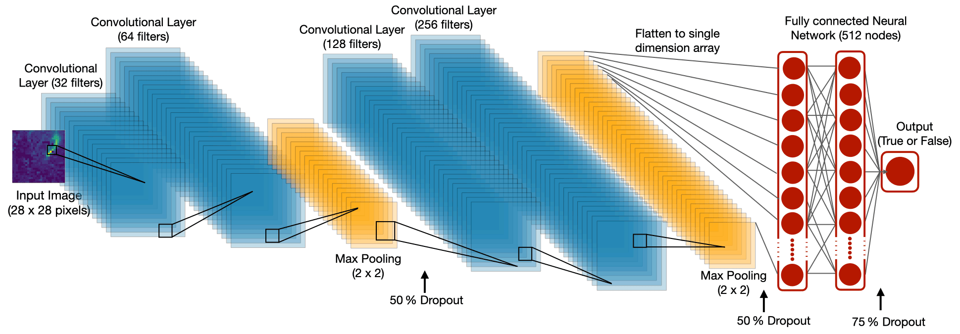
Figure 1Simplified schematic of the convolutional neural network architecture to identify NO2 plumes. See main text for further details.
Figure 1 shows a simplified schematic of the CNN architecture we use to create our plume identification model. The input image is first passed through two convolutional layers with 32 and 64 filters, respectively, followed by a maximum pooling layer. We then randomly drop 50 % of the layers from the model, which helps to prevent overfitting of the data (as recommended by Srivastava et al., 2014). The remaining data are then passed through two more convolutional layers of 128 and 256 filters, respectively, and another maximum pooling layer. This is followed by dropping another 50 % of the layers and flattening the array to one dimension to be fed into the FC layer that contains 512 nodes. Each CNN layer is then passed into a rectified linear unit (ReLU) activation function before going into the next layer. The last FC is passed into a softmax function to calculate the probabilities that the image contains a plume or not. The optimizer used here is an AdamOptimizer, which helps to reduce the cost calculated by cross-entropy. The model has a total of 4 892 770 trainable parameters.
Supervised learning strategy
To train our CNN model we use example images of TROPOMI NO2 that can be classified as containing a plume or not. Each image is 28 × 28 pixels (approximately corresponding to 200 km × 100 km) and was individually normalized to remove the influence of the magnitude of NO2 features, a step that also ensures the model parameters have a similar data distribution and therefore improves the model efficiency and accuracy. We acknowledge that normalizing each individual image could potentially lead to false detection if the background noise resembles a plume; the alternative of normalizing the images to a standard value decreases the model's ability to detect smaller emission sources and may lead to a larger number of false negatives. Figure 2 shows three example images from the level 2 TROPOMI NO2 data considered to contain plumes used in the training dataset. For an emission source to create a plume detectable by TROPOMI, the source must be subject to winds strong enough to disperse the emissions across multiple pixels within the lifetime of NO2. We anticipate that the number of occurrences where these conditions are not met will be relatively small compared to the entire dataset and therefore should not have an adverse effect on our results.
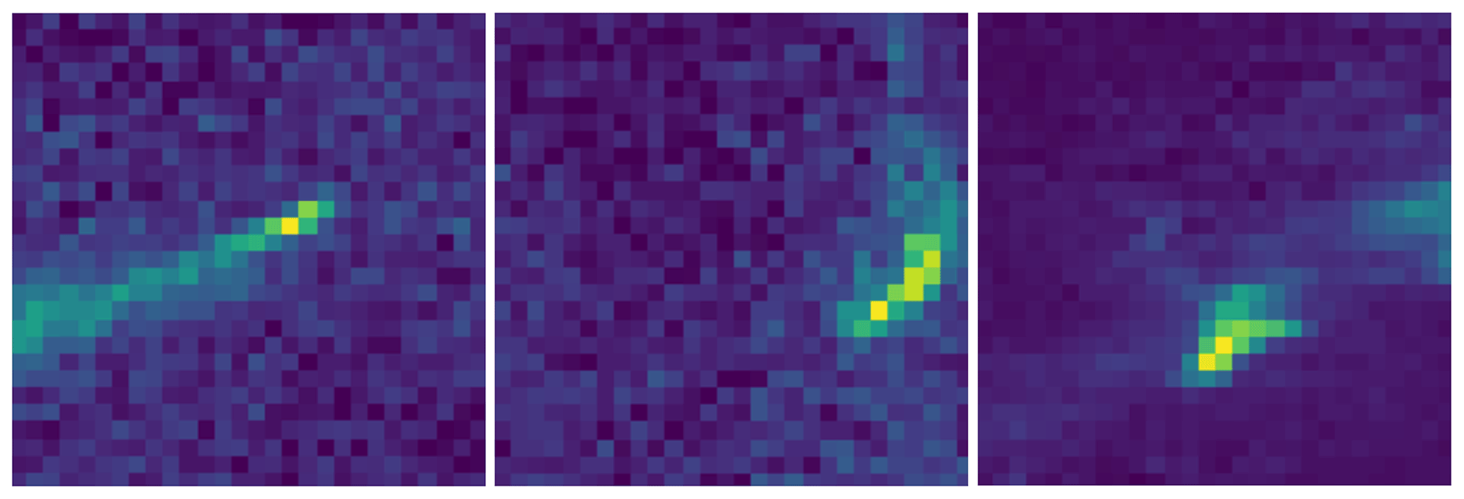
Figure 2Three examples of individually normalized images of TROPOMI tropospheric column NO2 that contain a plume.
Determining whether an image contains a plume or not is a non-trivial task that is subject to human judgement and is consequently prone to error. Plumes are highly variable in both size and shape and can potentially be obscured by other features in the image; in some instances, multiple plumes can be found within a single image. In the first instance, we used a crowd-sourcing approach where participants were asked to determine whether an image contained a plume. A total of 41 participants classified 1565 unique images and created 13 750 classifications, a mean of 8.8 classifications per image. This is further described in Appendix A. However, we found that this approach did not produce consistent results, with a larger number of images inconclusively classified by the participants than the number of images for which the participants agreed. This result emphasizes the role of human bias in identifying plumes, which in the absence of any post-training check compromises the performance of the CNN model.
Due to the lack of agreement in our crowd-sourced approach to plume identification, we created a dataset for this study based on the authors' judgement. Subjective judgement of the images could lead to small variations in repeated experiments, and therefore a more rigorous approach may be needed for future applications. We selected a total of 6086 images (3043 of which contained a plume) from across the globe for all times of year to minimize regional and seasonal biases. We used an iterative process to select images to train the model. We started with an initial set of images, randomly selected images that contained at least one plume, and corrected the classification if necessary, ensuring an equal number of true and false images were included in the training set. The images were then randomly split in an 80 : 20 ratio to train the CNN model and test the trained model. We find that the resulting CNN model achieves an accuracy of > 90 % when compared against the test data.
Using the developed plume identification model, we processed 2 years (July 2018–June 2020) of TROPOMI tropospheric NO2 data, resulting in 18 million individual 28 × 28 pixel images. Prior to running the model, we discarded images that included > 40 % invalid pixels, i.e. data that did not match the TROPOMI quality threshold as described above; this quality control step reduced the number of processed images to approximately 7.2 million. We then passed these images to our CNN model, which returned a Boolean variable that describes whether a plume was identified and an associated confidence level associated with the identification. We discard images for which the confidence threshold < 75 %. We find that our results are moderately sensitive to this value, with an approximate 10 % change in the number of plumes found when changing the confidence threshold by ±15 %. This confidence threshold can be adjusted to increase the number of identified plumes but at the expense of the confidence of the plumes being reported. For each image in which a plume was identified, we extract the geographical coordinates of the plume by identifying the image pixel with the maximum value. We acknowledge that this method could lead to inaccuracies as the maximum pixel value in the image will not necessarily correspond to the origin of the plume and may not identify all plumes (e.g. images that contain multiple plumes), but we consider this to be a minor source of error. The area of one TROPOMI NO2 pixel is approximately 24 km2, so the plume origin could easily fall within this area. Each image has an associated timestamp from the satellite, allowing us to build a dataset of the location and time of plumes spotted by TROPOMI.
First, we assess the performance of the CNN model to identify plumes on global and regional spatial scales. We then use the locations of these plumes to study their ability to identify anthropogenic combustion sources of CO2.
3.1 CNN model performance
Over our 2-year study period, the CNN model identified 310 020 images that contained at least one plume. After extracting the geographical locations for each plume location, we identified 62 040 (20 %) images that were within 15 km of an active fire as determined by VIIRS thermal anomaly data and categorize these NO2 plumes as being associated with biomass burning. We assign the remaining 247 980 NO2 plumes as originating from anthropogenic combustion.
3.1.1 Global-scale plume distributions
Figure 3 shows the location of NO2 plumes from fossil fuel and biomass burning over our study period. We find that anthropogenic combustion is widespread across the globe (Fig. 3a), with a focus over northern mid-latitudes, India and China, as expected. We also find coherent distributions of NO2 plumes over the ocean along established shipping routes. On the global scale, this is particularly noticeable in the Bay of Bengal between southern India and Southeast Asia and between the Cape of Good Hope, north-western Africa, and eastern Brazil. Shipping lanes are clearer on the regional scales we report below.
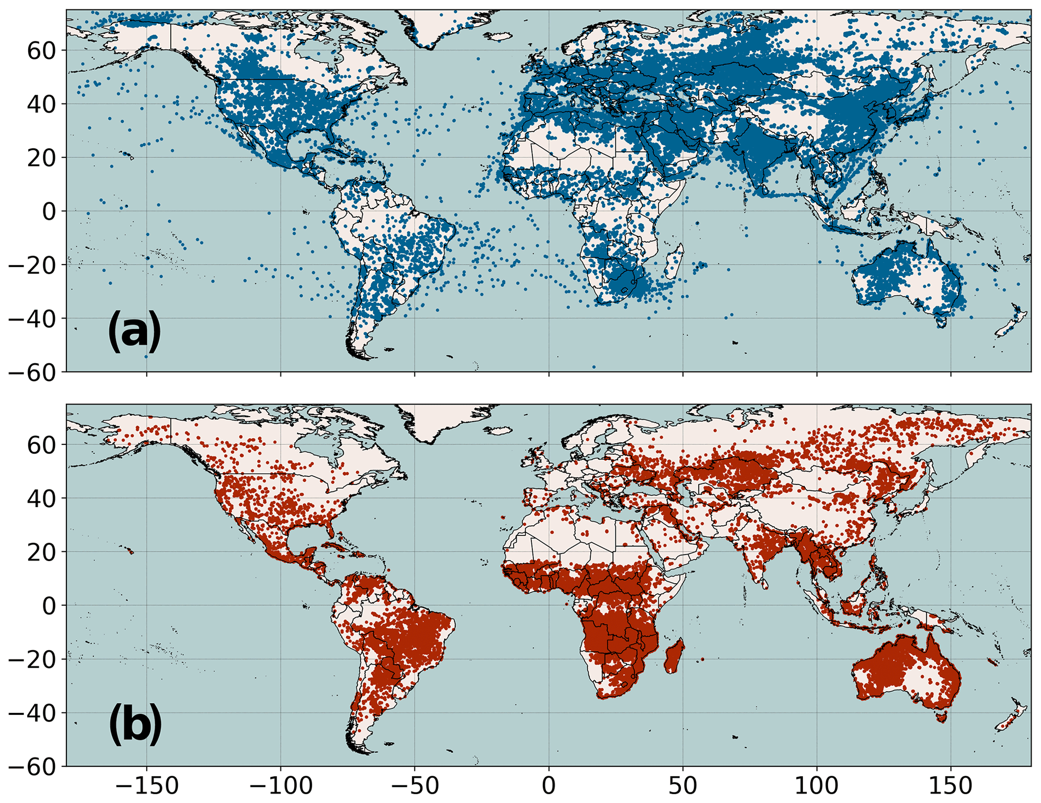
Figure 3Geographical locations of individual TROPOMI NO2 plumes identified using a CNN model, July 2018–June 2020. We attribute these plumes to (a) anthropogenic combustion or (b) biomass burning, depending on whether the plume falls within 15 km of the nearest VIIRS thermal anomaly measurement.
The cluster of plumes over northern Alaska (Fig. 3a) is an excellent example of a geographic region where NO2 emissions are dwarfed compared to other point sources on a global scale, so it will not typically appear as a hotspot using other detection methods. We believe these are genuine detections, which we link to petroleum extraction activities in the National Petroleum Reserve–Alaska in the Alaska North Slope region.
The distribution of biomass burning NO2 plumes (Fig. 3b) identified using the CNN model and VIIRS data highlights geographical regions where we expect seasonal fire activity, with a high density of plumes over western, central, and eastern Africa; Colombia; Venezuela; Brazil; and Australia. We account for the seasonal variation in fire activity by using daily VIIRS data and remove fire-influenced scenes from those identified by our CNN.
We acknowledge that a number of plumes that we classify as anthropogenic combustion occur in locations where we expect biomass burning, e.g. central Australia, various regions across the tropics, Siberia, and North America. We also acknowledge that anthropogenic plumes could be incorrectly labelled as biomass burning, especially where these emission types are co-located. While this suggests that our use of VIIRS is imperfect, we find that our approach broadly achieves its goal.
3.1.2 Regional-scale plume distributions
Figure 4 shows anthropogenic combustion plumes we identify from July 2018 to June 2020 over Europe, the contiguous US and southern Canada, China, and the Middle East. We have broadly classified these hotspots as major urban areas, power stations, and flaring regions. We identify major urban areas (populations > 200 000) based on data from https://www.naturalearthdata.com/downloads/10m-cultural-vectors/10m-populated-places/ (last access: 10 March 2021), fossil fuel power stations taken from the Global Power Plant Database (https://datasets.wri.org/dataset/globalpowerplantdatabase, last access: 10 March 2021, Byers et al., 2019), and oil and gas flaring regions based on data from https://skytruth.org/flaring/ (last access: 10 April 2021). We acknowledge that the power station database will be incomplete due to data availability and reliability across the globe (Byers et al., 2019). The location of oil and gas flaring used here, determined by nighttime thermal anomaly data from VIIRS, is clustered spatially and temporally and therefore may not coincide with the TROPOMI local overpass time of 13:30.
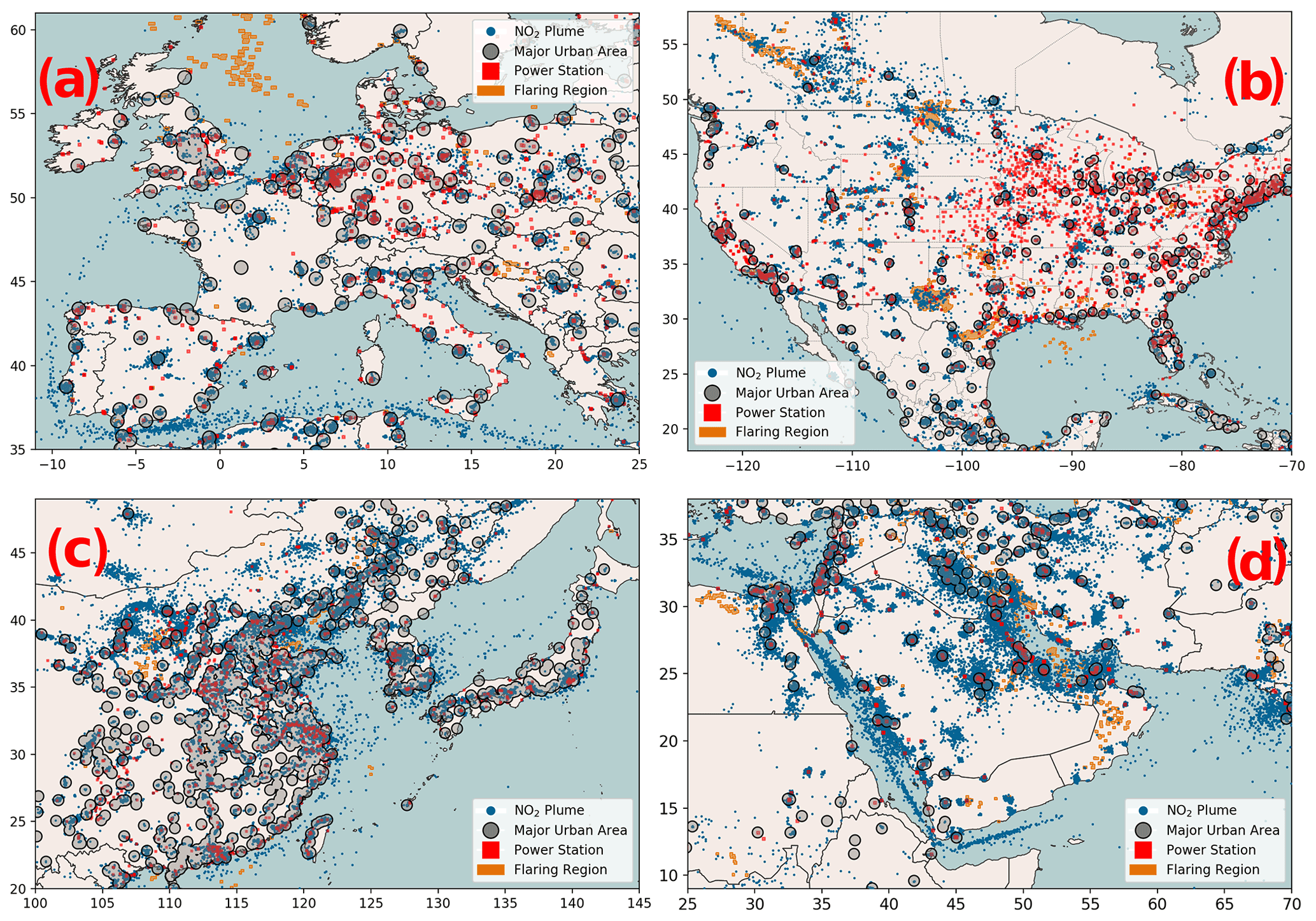
Figure 4Geographical locations of individual anthropogenic combustion plumes (denoted by blue dots) identified from TROPOMI tropospheric-NO2-column data using a CNN model, July 2018–June 2020. (a) Europe, (b) North America, (c) China, and (d) the Middle East. Also shown are the locations of major urban areas (populations > 200 000) denoted by grey circles; coal, oil and nature gas power stations denoted by red squares; and oil and gas flaring locations denoted by orange rectangles.
We find that the highest-density plumes are found over large cities, e.g. Paris, Madrid, Riyadh, Beijing, Los Angeles, and New York, and over busy ports such as Rotterdam, Porto, Cairo, and Hong Kong (Fig. 4a, b, c). Ship tracks are clearly seen through the Strait of Gibraltar (Fig. 4a) and the Red Sea leading to the Suez Canal (Fig. 4d). Plumes over China, Korea, and Japan are so dense they begin to overlap (Fig. 4c). We also find clusters of NO2 plumes over and around power stations and flaring regions, with some notable exceptions, e.g. North Sea oil fields (Fig. 4a), the oil fields in Oman and north-western Egypt (Fig. 4d), and the large number of power stations in the Midwestern United States (Fig. 4b). The poor correspondence between flaring regions and NO2 plumes may be due to differences in the overpass times of the data used, as discussed above. In general, the location of the NO2 plumes and the coincidence with cities, power plants and established shipping routes provide us with confidence of the CNN model we have developed. Discrepancies between known sources and the large areas of clustered NO2 plumes, especially over China and India, and power plants that do not have any associated plumes suggest that inventories being used to identify power plants are out of date. Further discrepancies may be due to detecting sources outwith the inventories used in this analysis (e.g. small settlements with large industrial emissions). Achieving this level of detail using conventional plume detection methods would be difficult.
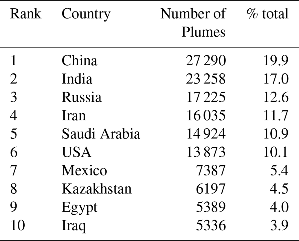
Table 1 shows the top 10 countries with the most fossil fuel plumes identified over the 2-year study period. China contains the most plumes, representing 20 % of all the plumes found during our study period. These plumes are mainly located around the highly urbanized and heavily industrial east of China (Fig. 4c), encompassing Beijing, Hebei, and Shenyang in the north-east. India is a close second with 17 %, where most plumes are over New Delhi, Mundra Port in the north-western Gujarat region and large coal mining areas to the north-east of the country (Fig. 3a). Russia is responsible for 12 % of plumes, spread over multiple cities and fossil fuel extraction works across the west of the country. The Middle East, including Iran, Saudi Arabia, and Iraq, is collectively responsible for more than 26 % of plumes. These plumes are mostly coincident with known regions of petroleum extraction and processing. Values over eastern Egypt appear to follow the Nile and abruptly stop before Sudan. Plumes over the US mainly coincide with major urban areas and flaring regions, with clusters found over some of the major oil and gas extraction sites, e.g. San Juan Basin, Permian Basin, Niobrara Formation, and Bakken Formation. There is also some evidence of oil and gas extraction over Mexico, e.g. Burro-Picachos and Sabinas, and over Kazakhstan, e.g. the Aktobe oil fields.
Table 1Top 10 countries containing the most fossil fuel plumes identified by TROPOMI NO2 plumes, July 2018–June 2020.
We acknowledge that statistics reported here will reflect the number of cloud-free days over specific regions. The frequency of global plume detections does change every month but does not show any seasonal cycle (not shown), even though there is a seasonal cycle of plume detections at high latitudes due to low sun angles during winter. Over our study period, the monthly mean number of fossil fuel NO2 plumes is 11 100, and the monthly mean number of biomass burning NO2 plumes is 2787. The largest number of fossil fuel plumes and biomass burning plumes was found during March 2019 and August 2018, respectively. Persistence of plume detection locations (Fig. 4) provides confidence that we are observing point sources. We find a total of 21 802 plumes detected over the oceans, mostly focused along ships tracks.
Table 2 shows the 20 cities across the globe with the most fossil fuel plumes identified over our 2-year study period. As previously discussed, cities that are likely to have more high-quality (cloud-free) retrievals are more likely to have plumes spotted over them; however the list of cities with the largest number of plumes is as expected based on knowledge of their large emissions. All of these 20 cities are within latitudes 35∘ S–35∘ N. Five of the cities are in India, with two each in neighbouring Pakistan and Bangladesh. Los Angeles and Phoenix are the only two US cities on the list, and there are two in Mexico (Mexico City and Torreón) and two in South America (Buenos Aires and Santiago). The others are in northern Africa (Cairo, Egypt, and Khartoum, Sudan), Indonesia, and South Korea. No cities in China are found in the top 20 despite most plumes being found in the country. We attribute this to large areas of industry in China being located outwith city boundaries.
Table 2Top 20 cities containing the most fossil fuel plumes over the study period.

3.2 What fraction of anthropogenic CO2 emissions are identified using NO2 plumes?
The low frequency of corresponding TROPOMI NO2 measurements and satellite observations of CO2 precludes any meaningful statistical analysis of CO2 : NO2 (not shown). We anticipate that this will improve with the launch of new satellites, particularly with the Copernicus CO2 constellation (CO2M) due for launch in 2025 and the Japanese Global Observing SATellite for Greenhouse gases and Water cycle (GOSAT-GW) due for launch in 2023.
To help us understand the fraction of global anthropogenic CO2 emissions that are identified using our plume identification model, we sample the Open-source Data Inventory for Anthropogenic CO2 (ODIAC; 2020 release; Oda and Maksyutov, 2011; Oda et al., 2018; Oda and Maksyutov, 2021) where there is an NO2 plume. We use the monthly 1∘ × 1∘ ODIAC gridded land CO2 emissions dataset for 2018 and 2019, and in the absence of 2020 data we use the 2019 ODIAC emissions for January–June 2020 to compare against the plume dataset. We do not anticipate that the COVID-19-related lockdowns of 2020 will significantly impact our results as the reduction in CO2 emissions was less than expected (Tollefson, 2021). We sample the ODIAC dataset between −50–50∘ north to remove the impact of fewer observations during winter months. For this comparison, we assume that all anthropogenic combustion sources of CO2 in the ODIAC dataset co-emit NO2 and therefore can be used as geographical validation for the plume detection dataset.
We sample the ODIAC dataset at the location and month of each NO2 plume identified using our model. Figure 5 shows the cumulative percentage of total emissions and the corresponding emission rate described as a function of the percentage of sources (from large to small) for the entire ODIAC dataset and the ODIAC dataset sampled at the NO2 plume locations. We find that for ODIAC emissions, large sources (> 1 g C m−2 d−1) account for approximately 25 % of all sources but contribute approximately 90 % of the total emissions. The ODIAC emissions sampled by the NO2 plumes accounted for 92 % of all global CO2 emissions, described by 56 % of all sources. The remaining 8 % of emissions, described by 44 % of all sources, typically have values of < 0.18 g C m−2 d−1. This suggests that our method of identifying NO2 plumes is biased towards the largest end of the emission spectrum and is less sensitive to the smallest emissions. This limit of detection does not lead to a large discrepancy in the total emissions being sampled by the NO2 plumes, reflecting the disproportionate role of large emission sources in the total emission budget.
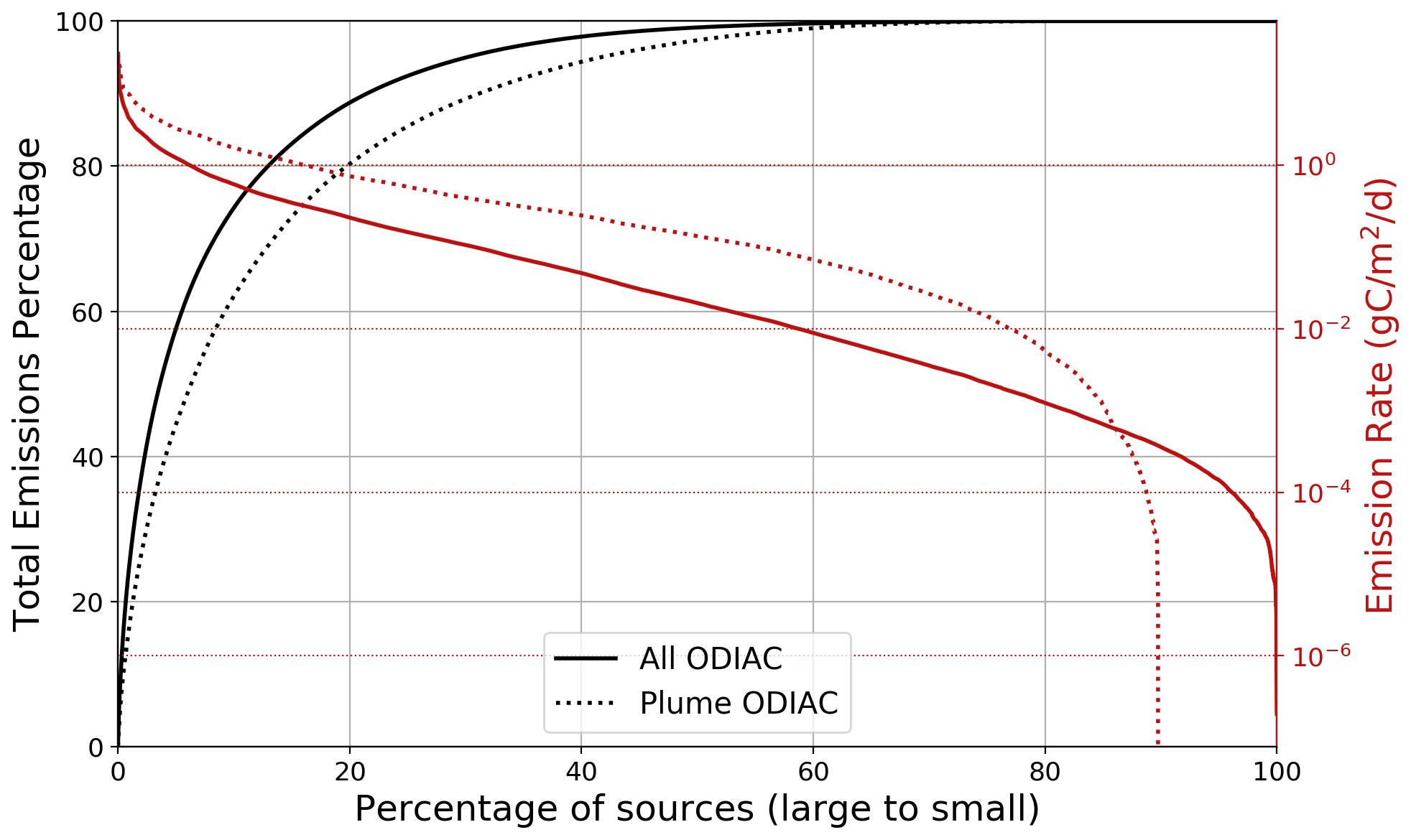
Figure 5The cumulative total emission percentage as a function of source size (black) and emission rate as a function of source size (red) for all ODIAC (solid line) and ODIAC sampled at plume locations (dotted line).
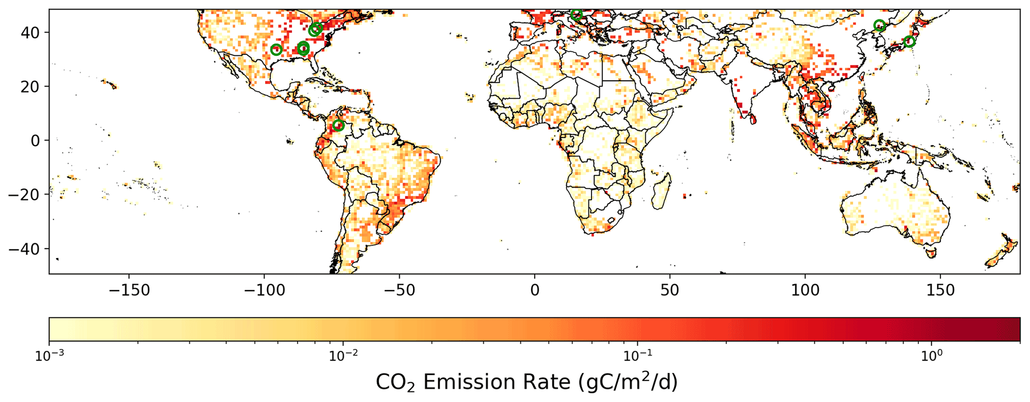
Figure 6CO2 emission rates as per the ODIAC inventory where no plumes were detected. The green circles indicate sources greater than 1 g C m−2 d−1.
Figure 6 shows the ODIAC emissions where no NO2 plumes were detected. Out of these undetected sources, 95 % have emission rates < 0.18 g C m−2 d−1, and only nine locations have an emission rate > 1 g C m−2 d−1, denoted by the green circles. Five of these locations are situated in the USA, with the remaining in Colombia, China, Japan, and Slovenia. The locations in the USA are all between large cities, connected by highways that are not described by single point sources. The source in Colombia is located in an area of persistent cloud cover (> 80 % of the year) and therefore will have fewer high-quality observations from TROPOMI. The reason for the missed large sources over China, Japan, and Slovenia is unclear.
Figure 5 also shows that 10 % of our plumes do not correspond to ODIAC CO2 emissions. This is due mostly to plumes over the ocean associated with ship tracks (Figs. 3 and 4), but there will be instances where fires have not been removed using our VIIRS criterion (described above) and possibly false detections. Here, we also consider the possibility that the emission inventory is incomplete for some reason.
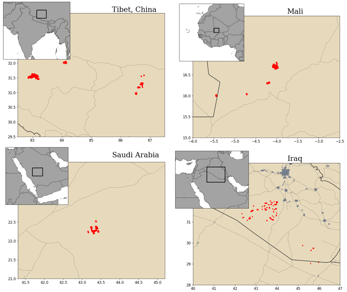
Figure 7Example locations with plume clusters that are not associated with ODIAC CO2 emissions. The light-grey lines show major roads, and urban areas are shown by grey patches.
Figure 7 shows four examples of clusters of plumes spotted by the detection method which do not have any associated ODIAC emissions. The clustering of the plumes suggests that they are highly unlikely to be false detections, and the persistence of the features over multiple years suggests that it is unlikely to be biomass burning. Although accurate determination of the emissions associated with these hotspots is outside the scope of this paper, we hypothesize based on satellite imagery from Google Maps that these are regions of fossil fuel extraction and processing (coal in China and oil and gas in Mali, Saudi Arabia, and Iraq). Having the ability to detect these plumes automatically provides a method of frequently updating emission inventories. Although these clusters of plumes could be persistent errors from highly reflective features such as salt lakes and solar panels, it is unlikely that they would appear as plume-shaped anomalies and therefore are less likely to be picked up by the CNN model. As well as errors in the TROPOMI retrieval leading to false detections in the final dataset, errors may also occur during the creation of the model (e.g. mislabelled training data). A single plume data point may not represent a real-life plume and should be considered in the context of other data (e.g. frequent recurrence, land use, proximity to other sources). Further refinement of the training dataset, model parameters, and data analysis stages will reduce the number of false detections, and feedback to the TROPOMI community could help reduce the number of retrieval errors.
We have developed a convolutional neural network (CNN) to identify plumes of atmospheric nitrogen dioxide (NO2), a tracer of combustion. We have trained the model using a small subset of available images from the TROPOspheric Monitoring Instrument, aboard Sentinel-5P. The resulting CNN, capable of identifying plumes with a success rate > 90 %, reveals a rich distribution of plumes across the globe, which correspond to large city centres, power plants, oil and gas production, and shipping routes. Many of these features would be difficult to isolate without the use of a deep learning model.
The impetus for our study is using NO2 as a tracer for anthropogenic emissions of CO2 and methane from combustion. We aim to demonstrate the potential of this method to exploit NO2 observations in conjunction with other relevant data and known relationships with gases such as CO2 and methane to improve emission estimates. The main advantage of using NO2 is its comparatively short atmospheric lifetime, allowing elevated values to be related to local emissions. We have attempted to remove biomass burning using thermal anomaly data, which are often used to locate open biomass burning. This is not a perfect method, but our results suggest that it works reasonably well. To evaluate our ability to observe anthropogenic emissions of CO2 we have used the Open-Data Inventory for Anthropogenic Carbon dioxide (ODIAC) (Oda et al., 2018), an established emission inventory used widely by the community. We have chosen this approach because we found the number of coincident measurements of TROPOMI NO2 and OCO-2/GOSAT CO2 was not sufficient to generate meaningful statistics (not shown). By sampling ODIAC at the location of NO2 plumes, we find that the CNN model describes 92 % of global anthropogenic CO2 emissions. The remaining 8 % of emissions, mostly < 0.2 g C m−2 d−1, provide an effective limit of detection for our method.
Our use of NO2 to describe anthropogenic emissions of CO2 and methane relies on them being co-emitted. We find no evidence in the literature of NOx scrubbers being used for power plants, although they are used by the chemical industry, which is a sector that represents a comparatively small emission of CO2. The validity of using NO2 as a proxy for CO2 emissions may change in the future as non-catalytic reduction and low-NOx burner technologies begin to mature. We find no correlation between NO2 plumes and the location of natural gas flaring, which is unexpected since this will be a major form of combustion and therefore should result in a significant source of NO2. We have no explanation for this observation, except if flaring occurs at preferential times of day that do not coincide with the early afternoon overpass time of TROPOMI. Our approach will also miss direct CO2 and methane emissions, e.g. pipeline leaks, coal mines (Palmer et al., 2021). For these sources, we still have to rely on highly spatially resolved CO2 and methane data (Varon et al., 2021). In contrast, we also find persistent NO2 plumes from regions where ODIAC does not currently include CO2 emissions that may be real or reflect false positives. False positives can result from data retrieval errors or from human error in the supervised learning strategy necessary to develop the CNN model. Based on the location and inspection of satellite imagery provided by Google Maps we suggest that these are likely to be associated with new areas where fossils fuels are being extracted or combusted for energy generation. This demonstrates how NO2 plumes could be used to inform emission inventories about the location of new point sources across the globe. Generally, it is important for domain-level expertise to evaluate data products developed by deep learning models to minimize the influence of false positives.
The NO2 plume detection algorithm does not quantify anthropogenic emissions of CO2 or methane, but it provides a method to refine the development of measurement, reporting and verification systems that form the backbone of the Paris Agreement. The launch of the Copernicus CO2 service, including a constellation of satellites that will measure CO2, methane, and NO2, will result in a step change in the number of coincident measurements and will thereby improve our ability to simultaneously use NO2 with CO2 and methane to quantify anthropogenic emissions of CO2 and methane.
We created a temporary online tool that briefly describes what a plume is with a few examples of what they can look like and then displays 18 images in a 6 × 3 grid. These images were selected at random from an initial 1565 unique images which were compiled by the authors. Each participant was then invited to click on the images in the grid which they considered to contain a plume and then to submit their selection. Once their results were submitted, the participant was asked to classify 18 more random images. We then used these results to determine how many true (contains a plume) or false (does not contain a plume) classifications each image received. We designed this method to reduce the amount of human error and individual judgement on what could be considered a plume or not.
A total of 41 participants classified 1565 unique images and created 13 750 classifications, a mean of 8.8 classifications per image. The number of classifications per participant is unknown as this was an online tool open to the public and relied on how much time they were willing to give.
For this crowd sourcing experiment, there were approximately 580 images for which 0 %–10 % of classifications were true, i.e. high confidence that these images do not contain a plume. There were approximately 130 images for which 90 %–100 % of classifications were true. For the remaining (≃ 800) images there was little agreement between the participants about whether they included a plume or not. Since the majority of the images from the initial dataset did not have a high level of agreement on whether they contained a plume or not, we decided that this dataset was not suitable to train our model.
Going forward, this experiment could be refined to help improve the results and give us more confidence in the classifications of the images. The experiment assumed that all images did not contain a plume unless the participant changed the classification; this meant that if a participant did not see an image then it would be considered not to contain a plume. We also noticed that what was considered a plume changed depending on the surrounding images. If the participant is unsure whether an image contains a plume or not, they may be more likely to keep the image classification as false if a surrounding image contained a clearer plume or vice versa if the surrounding images definitely did not contain a plume.
TROPOMI NO2 data are available from https://doi.org/10.5270/S5P-s4ljg54 (European Space Agency, 2021), VIIRS biomass burning data are available from https://firms.modaps.eosdis.nasa.gov/download/ (Schroeder et al., 2014), and the ODIAC emission dataset is available from https://doi.org/10.17595/20170411.001 (Oda and Maksyutov, 2015).
DPF and PIP designed the research; DPF prepared the calculations with initial input from TZ; DPF and PIP analysed the results and wrote the paper, with comments from TZ.
The contact author has declared that neither they nor their co-authors have any competing interests.
Publisher’s note: Copernicus Publications remains neutral with regard to jurisdictional claims in published maps and institutional affiliations.
Douglas P. Finch, Paul I. Palmer, and Tianran Zhang gratefully acknowledge funding from the National Centre for Earth Observation funded by the National Environment Research Council (NE/R016518/1).
This research has been supported by the National Centre for Earth Observation (grant no. NE/R016518/1).
This paper was edited by Michel Van Roozendael and reviewed by two anonymous referees.
Boersma, K. F., Eskes, H. J., Dirksen, R. J., van der A, R. J., Veefkind, J. P., Stammes, P., Huijnen, V., Kleipool, Q. L., Sneep, M., Claas, J., Leitão, J., Richter, A., Zhou, Y., and Brunner, D.: An improved tropospheric NO2 column retrieval algorithm for the Ozone Monitoring Instrument, Atmos. Meas. Tech., 4, 1905–1928, https://doi.org/10.5194/amt-4-1905-2011, 2011. a
Bovensmann, H., Buchwitz, M., Burrows, J. P., Reuter, M., Krings, T., Gerilowski, K., Schneising, O., Heymann, J., Tretner, A., and Erzinger, J.: A remote sensing technique for global monitoring of power plant CO2 emissions from space and related applications, Atmos. Meas. Tech., 3, 781–811, https://doi.org/10.5194/amt-3-781-2010, 2010. a
Broquet, G., Bréon, F.-M., Renault, E., Buchwitz, M., Reuter, M., Bovensmann, H., Chevallier, F., Wu, L., and Ciais, P.: The potential of satellite spectro-imagery for monitoring CO2 emissions from large cities, Atmos. Meas. Tech., 11, 681–708, https://doi.org/10.5194/amt-11-681-2018, 2018. a
Brunner, D., Kuhlmann, G., Marshall, J., Clément, V., Fuhrer, O., Broquet, G., Löscher, A., and Meijer, Y.: Accounting for the vertical distribution of emissions in atmospheric CO2 simulations, Atmos. Chem. Phys., 19, 4541–4559, https://doi.org/10.5194/acp-19-4541-2019, 2019. a
Byers, L., Friedrich, J., Hennig, R., Kressig, A., McCormick, C., and Malaguzzi Valeri, L.: A Global Database of Power Plants, Resource Watch, available at: https://datasets.wri.org/dataset/globalpowerplantdatabase (last access: 10 March 2021), 2019. a, b
de Gouw, J. A., Veefkind, J. P., Roosenbrand, E., Dix, B., Lin, J. C., Landgraf, J., and Levelt, P. F.: Daily Satellite Observations of Methane from Oil and Gas Production Regions in the United States, Sci. Rep., 10, 1379, https://doi.org/10.1038/s41598-020-57678-4, 2020. a
Duren, R. M., Thorpe, A. K., Foster, K. T., Rafiq, T., Hopkins, F. M., Yadav, V., Bue, B. D., Thompson, D. R., Conley, S., Colombi, N. K., Frankenberg, C., McCubbin, I. B., Eastwood, M. L., Falk, M., Herner, J. D., Croes, B. E., Green, R. O., and Miller, C. E.: California's methane super-emitters, Nature, 575, 180–184, https://doi.org/10.1038/s41586-019-1720-3, 2019. a
Edenhofer, O., Pichs-Madruga, R., Sokona, Y., Farahani, E., Kadner, S., Seyboth, K., Adler, A., Baum, I., Brunner, S., Eickemeier, P., Kriemann, B., Savolainen, J., Schlömer, S., von Stechow, C., Zwickel, T., and Minx, J. C. (Eds.): Climate Change 2014: Mitigation of Climate Change, Contribution of Working Group III to the Fifth Assessment Report of the Intergovernmental Panel on Climate Change, Cambridge University Press, 2014. a
European Space Agency: Copernicus Sentinel-5P, TROPOMI Level 2 Nitrogen Dioxide total column products, European Space Agency [data set], https://doi.org/10.5270/S5P-s4ljg54, 2021. a
Friedlingstein, P., O'Sullivan, M., Jones, M. W., Andrew, R. M., Hauck, J., Olsen, A., Peters, G. P., Peters, W., Pongratz, J., Sitch, S., Le Quéré, C., Canadell, J. G., Ciais, P., Jackson, R. B., Alin, S., Aragão, L. E. O. C., Arneth, A., Arora, V., Bates, N. R., Becker, M., Benoit-Cattin, A., Bittig, H. C., Bopp, L., Bultan, S., Chandra, N., Chevallier, F., Chini, L. P., Evans, W., Florentie, L., Forster, P. M., Gasser, T., Gehlen, M., Gilfillan, D., Gkritzalis, T., Gregor, L., Gruber, N., Harris, I., Hartung, K., Haverd, V., Houghton, R. A., Ilyina, T., Jain, A. K., Joetzjer, E., Kadono, K., Kato, E., Kitidis, V., Korsbakken, J. I., Landschützer, P., Lefèvre, N., Lenton, A., Lienert, S., Liu, Z., Lombardozzi, D., Marland, G., Metzl, N., Munro, D. R., Nabel, J. E. M. S., Nakaoka, S.-I., Niwa, Y., O'Brien, K., Ono, T., Palmer, P. I., Pierrot, D., Poulter, B., Resplandy, L., Robertson, E., Rödenbeck, C., Schwinger, J., Séférian, R., Skjelvan, I., Smith, A. J. P., Sutton, A. J., Tanhua, T., Tans, P. P., Tian, H., Tilbrook, B., van der Werf, G., Vuichard, N., Walker, A. P., Wanninkhof, R., Watson, A. J., Willis, D., Wiltshire, A. J., Yuan, W., Yue, X., and Zaehle, S.: Global Carbon Budget 2020, Earth Syst. Sci. Data, 12, 3269–3340, https://doi.org/10.5194/essd-12-3269-2020, 2020. a
Gurney, K. R., Liang, J., Roest, G., Song, Y., Mueller, K., and Lauvaux, T.: Under-reporting of greenhouse gas emissions in U.S. cities, Nat. Commun., 12, 553, https://doi.org/10.1038/s41467-020-20871-0, 2021. a
Hakkarainen, J., Ialongo, I., and Tamminen, J.: Direct space‐based observations of anthropogenic CO2 emission areas from OCO‐2, Geophys. Res. Lett., 43, 11400–11406, https://doi.org/10.1002/2016GL070885, 2016. a
Hakkarainen, J., Szela̧g, M. E., Ialongo, I., Retscher, C., Oda, T., and Crisp, D.: Analyzing nitrogen oxides to carbon dioxide emission ratios from space: A case study of Matimba Power Station in South Africa, Atmos. Environ. X, 10, 100110, https://doi.org/10.1016/j.aeaoa.2021.100110, 2021. a
Ialongo, I., Stepanova, N., Hakkarainen, J., Virta, H., and Gritsenko, D.: Satellite-based estimates of nitrogen oxide and methane emissions from gas flaring and oil production activities in Sakha Republic, Russia, Atmos. Environ. X, 11, 100114, https://doi.org/10.1016/j.aeaoa.2021.100114, 2021. a
International Marine Organization: Fourth IMO Greenhouse Gas Study, Tech. rep., International Marine Organization, 2020. a
Janssens-Maenhout, G., Pinty, B., Dowell, M., Zunker, H., Andersson, E., Balsamo, G., Bézy, J.-L., Brunhes, T., Boesch, H., Bojkov, B., Brunner, D., Buchwitz, M., Crisp, D., Ciais, P., Counet, P., Dee, D., van der Gon, H. D., Dolman, H., Drinkwater, M. R., Dubovik, O., Engelen, R., Fehr, T., Fernandez, V., Heimann, M., Holmlund, K., Houweling, S., Husband, R., Juvyns, O., Kentarchos, A., Landgraf, J., Lang, R., Löscher, A., Marshall, J., Meijer, Y., Nakajima, M., Palmer, P. I., Peylin, P., Rayner, P., Scholze, M., Sierk, B., Tamminen, J., and Veefkind, P.: Toward an Operational Anthropogenic CO2 Emissions Monitoring and Verification Support Capacity, B. Am. Meteorol. Soc., 101, E1439–E1451, https://doi.org/10.1175/BAMS-D-19-0017.1, 2020. a
Kort, E. A., Frankenberg, C., Miller, C. E., and Oda, T.: Space-based observations of megacity carbon dioxide, Geophys. Res. Lett., 39, L17806, https://doi.org/10.1029/2012GL052738, 2012. a
Kuhlmann, G., Broquet, G., Marshall, J., Clément, V., Löscher, A., Meijer, Y., and Brunner, D.: Detectability of CO2 emission plumes of cities and power plants with the Copernicus Anthropogenic CO2 Monitoring (CO2M) mission, Atmos. Meas. Tech., 12, 6695–6719, https://doi.org/10.5194/amt-12-6695-2019, 2019. a
Kuhlmann, G., Brunner, D., Broquet, G., and Meijer, Y.: Quantifying CO2 emissions of a city with the Copernicus Anthropogenic CO2 Monitoring satellite mission, Atmos. Meas. Tech., 13, 6733–6754, https://doi.org/10.5194/amt-13-6733-2020, 2020. a
Lary, D. J., Alavi, A. H., Gandomi, A. H., and Walker, A. L.: Machine learning in geosciences and remote sensing, Geosci. Front., 7, 3–10, https://doi.org/10.1016/j.gsf.2015.07.003, 2016. a
Liu, F., Duncan, B. N., Krotkov, N. A., Lamsal, L. N., Beirle, S., Griffin, D., McLinden, C. A., Goldberg, D. L., and Lu, Z.: A methodology to constrain carbon dioxide emissions from coal-fired power plants using satellite observations of co-emitted nitrogen dioxide, Atmos. Chem. Phys., 20, 99–116, https://doi.org/10.5194/acp-20-99-2020, 2020. a
Lorente, A., Folkert Boersma, K., Yu, H., Dörner, S., Hilboll, A., Richter, A., Liu, M., Lamsal, L. N., Barkley, M., De Smedt, I., Van Roozendael, M., Wang, Y., Wagner, T., Beirle, S., Lin, J.-T., Krotkov, N., Stammes, P., Wang, P., Eskes, H. J., and Krol, M.: Structural uncertainty in air mass factor calculation for NO2 and HCHO satellite retrievals, Atmos. Meas. Tech., 10, 759–782, https://doi.org/10.5194/amt-10-759-2017, 2017. a
Maxwell, A. E., Warner, T. A., and Fang, F.: Implementation of machine-learning classification in remote sensing: an applied review, Int. J. Remote Sens., 39, 2784–2817, https://doi.org/10.1080/01431161.2018.1433343, 2018. a
Nassar, R., Hill, T. G., McLinden, C. A., Wunch, D., Jones, D. B. A., and Crisp, D.: Quantifying CO2 Emissions From Individual Power Plants From Space, Geophys. Res. Lett., 44, 10045–10053, https://doi.org/10.1002/2017GL074702, 2017. a
Oda, T. and Maksyutov, S.: A very high-resolution (1 km × 1 km) global fossil fuel CO2 emission inventory derived using a point source database and satellite observations of nighttime lights, Atmos. Chem. Phys., 11, 543–556, https://doi.org/10.5194/acp-11-543-2011, 2011. a
Oda, T. and Maksyutov, S.: ODIAC Fossil Fuel CO2 Emissions Dataset (Version name: ODIAC2020b), Center for Global Environmental Research, National Institute for Environmental Studies, https://doi.org/10.17595/20170411.001, 2021. a
Oda, T. and Maksyutov, S.: ODIAC Fossil Fuel CO2 Emissions Dataset (Version name*1: ODIACYYYY or ODIACYYYYa), Center for Global Environmental Research, National Institute for Environmental Studies [data set], https://doi.org/10.17595/20170411.001, 2015. a
Oda, T., Maksyutov, S., and Andres, R. J.: The Open-source Data Inventory for Anthropogenic CO2, version 2016 (ODIAC2016): a global monthly fossil fuel CO2 gridded emissions data product for tracer transport simulations and surface flux inversions, Earth Syst. Sci. Data, 10, 87–107, https://doi.org/10.5194/essd-10-87-2018, 2018. a, b
Palmer, P. I., Feng, L., Lunt, M. F., Parker, R. J., Bösch, H., Lan, X., Lorente, A., and Borsdorff, T.: The added value of satellite observations of methane forunderstanding the contemporary methane budget, Philos. T. Roy. Soc. A, 379, 20210106, https://doi.org/10.1098/rsta.2021.0106, 2021. a
Poore, J. and Nemecek, T.: Reducing food's environmental impacts through producers and consumers, Science, 360, 987–992, https://doi.org/10.1126/science.aaq0216, 2018. a
Reuter, M., Buchwitz, M., Schneising, O., Krautwurst, S., O'Dell, C. W., Richter, A., Bovensmann, H., and Burrows, J. P.: Towards monitoring localized CO2 emissions from space: co-located regional CO2 and NO2 enhancements observed by the OCO-2 and S5P satellites, Atmos. Chem. Phys., 19, 9371–9383, https://doi.org/10.5194/acp-19-9371-2019, 2019. a
Schroeder, W., Oliva, P., Giglio, L., and Csiszar, I. A.: The New VIIRS 375 m active fire detection data product: algorithm description and initial assessment, Remote Sens. Environ., 143, 85–96, https://doi.org/10.1016/j.rse.2013.12.008, 2014 (data available at: https://firms.modaps.eosdis.nasa.gov/download/, last access: 18 March 2021). a
Srivastava, N., Hinton, G., Krizhevsky, A., Sutskever, I., and Salakhutdinov, R.: Dropout: A simple way to prevent neural networks from overfitting, J. Mach. Learn. Res., 15, 1929–1958, 2014. a
Strandgren, J., Krutz, D., Wilzewski, J., Paproth, C., Sebastian, I., Gurney, K. R., Liang, J., Roiger, A., and Butz, A.: Towards spaceborne monitoring of localized CO2 emissions: an instrument concept and first performance assessment, Atmos. Meas. Tech., 13, 2887–2904, https://doi.org/10.5194/amt-13-2887-2020, 2020. a
Tollefson, J.: COVID curbed carbon emissions in 2020 – but not by much, Nature, 589, 343–343, https://doi.org/10.1038/d41586-021-00090-3, 2021. a
van Geffen, J. H. G. M., Boersma, K. F., Van Roozendael, M., Hendrick, F., Mahieu, E., De Smedt, I., Sneep, M., and Veefkind, J. P.: Improved spectral fitting of nitrogen dioxide from OMI in the 405–465 nm window, Atmos. Meas. Tech., 8, 1685–1699, https://doi.org/10.5194/amt-8-1685-2015, 2015. a
Varon, D. J., McKeever, J., Jervis, D., Maasakkers, J. D., Pandey, S., Houweling, S., Aben, I., Scarpelli, T., and Jacob, D. J.: Satellite Discovery of Anomalously Large Methane Point Sources From Oil/Gas Production, Geophys. Res. Lett., 46, 13507–13516, https://doi.org/10.1029/2019GL083798, 2019. a
Varon, D. J., Jervis, D., McKeever, J., Spence, I., Gains, D., and Jacob, D. J.: High-frequency monitoring of anomalous methane point sources with multispectral Sentinel-2 satellite observations, Atmos. Meas. Tech., 14, 2771–2785, https://doi.org/10.5194/amt-14-2771-2021, 2021. a, b
Veefkind, J., Aben, I., McMullan, K., Förster, H., De Vries, J., Otter, G., Claas, J., Eskes, H., De Haan, J., Kleipool, Q., van Weele, M., Hasekamp, O., Hoogeveen, R., Landgraf, J., Snel, R., Tol, P., Ingmann, P., Voors, R., Kruizinga, B., Vink, R., Visser, H., and Levelt, P. F.: TROPOMI on the ESA Sentinel-5 Precursor: A GMES mission for global observations of the atmospheric composition for climate, air quality and ozone layer applications, Remote Sens. Environ., 120, 70–83, 2012. a
Wang, Y., Ciais, P., Broquet, G., Bréon, F.-M., Oda, T., Lespinas, F., Meijer, Y., Loescher, A., Janssens-Maenhout, G., Zheng, B., Xu, H., Tao, S., Gurney, K. R., Roest, G., Santaren, D., and Su, Y.: A global map of emission clumps for future monitoring of fossil fuel CO2 emissions from space, Earth Syst. Sci. Data, 11, 687–703, https://doi.org/10.5194/essd-11-687-2019, 2019. a
Wang, Y., Broquet, G., Bréon, F.-M., Lespinas, F., Buchwitz, M., Reuter, M., Meijer, Y., Loescher, A., Janssens-Maenhout, G., Zheng, B., and Ciais, P.: PMIF v1.0: assessing the potential of satellite observations to constrain CO2 emissions from large cities and point sources over the globe using synthetic data, Geosci. Model Dev., 13, 5813–5831, https://doi.org/10.5194/gmd-13-5813-2020, 2020. a
Wu, D., Lin, J. C., Oda, T., and Kort, E. A.: Space-based quantification of per capita CO2 emissions from cities, Environ. Res. Lett., 15, 035004, https://doi.org/10.1088/1748-9326/ab68eb, 2020. a
Yang, E. G., Kort, E. A., Wu, D., Lin, J. C., Oda, T., Ye, X., and Lauvaux, T.: Using Space‐Based Observations and Lagrangian Modeling to Evaluate Urban Carbon Dioxide Emissions in the Middle East, J. Geophys. Res.-Atmos., 125, e2019JD031922, https://doi.org/10.1029/2019JD031922, 2020. a
Ye, X., Lauvaux, T., Kort, E. A., Oda, T., Feng, S., Lin, J. C., Yang, E. G., and Wu, D.: Constraining Fossil Fuel CO2 Emissions From Urban Area Using OCO‐2 Observations of Total Column CO2, J. Geophys. Res.-Atmos., 125, e2019JD030528, https://doi.org/10.1029/2019JD030528, 2020. a
Zara, M., Boersma, K. F., De Smedt, I., Richter, A., Peters, E., van Geffen, J. H. G. M., Beirle, S., Wagner, T., Van Roozendael, M., Marchenko, S., Lamsal, L. N., and Eskes, H. J.: Improved slant column density retrieval of nitrogen dioxide and formaldehyde for OMI and GOME-2A from QA4ECV: intercomparison, uncertainty characterisation, and trends, Atmos. Meas. Tech., 11, 4033–4058, https://doi.org/10.5194/amt-11-4033-2018, 2018. a
Zheng, B., Chevallier, F., Ciais, P., Broquet, G., Wang, Y., Lian, J., and Zhao, Y.: Observing carbon dioxide emissions over China's cities and industrial areas with the Orbiting Carbon Observatory-2, Atmos. Chem. Phys., 20, 8501–8510, https://doi.org/10.5194/acp-20-8501-2020, 2020. a
Zheng, T., Nassar, R., and Baxter, M.: Estimating power plant CO2 emission using OCO-2 XCO2 and high resolution WRF-Chem simulations, Environ. Res. Lett., 14, 85001, https://doi.org/10.1088/1748-9326/ab25ae, 2019. a