Consistency test of precipitating ice cloud retrieval properties obtained from the observations of different instruments operating at Dome C (Antarctica)

Selected case studies of precipitating ice clouds at Dome C (Antarctic Plateau) were used to test a new approach for the estimation of ice cloud reflectivity at 24 GHz (12.37 mm wavelength) using ground-based far infrared spectral measurements from the REFIR-PAD Fourier transform spectroradiometer and backscattering/depolarization lidar profiles. The resulting reflectivity was evaluated with the direct reflectivity measurements provided by a co-located micro rain radar (MRR) operating at 24 GHz, that was able to detect falling crystals with large particle size, typically above 600 µm. To obtain the 24 GHz reflectivity, we used the particle effective diameter and the cloud optical depth retrieved from the far infrared spectral radiances provided by REFIR-PAD and the tropospheric co-located backscattering lidar to calculate the modal radius and the intercept of the particle size distribution. These parameters spanned in the wide ranges between 570–2400 µm and 10⁻²–10⁴ cm⁻⁵, respectively. The retrieved effective sizes and optical depths mostly varied in the ranges 70–250 µm and 0.1–5, respectively. From these parameters, the theoretical reflectivity at 24 GHz was obtained by integrating the size distribution over different cross sections for various habit crystals provided by Eriksson et al. (2018) databases. From the comparison with the radar reflectivity measurements, we found that the hexagonal column-like habits, the columnar crystal aggregates, and the $\mathrm{5}/\mathrm{6}$ branches bullet rosettes showed the best agreement with the MRR observations. The dispersion coefficient of the crystal particle size distribution was assumed in the range 0–2 according to the temperature dependence found in previous studies. The retrieved values of the intercept and slope were found in good agreement with these studies. The presence of the inferred habits was confirmed by the crystal images taken by the ICE-CAMERA, operating in proximity of REFIR-PAD and the MRR. In particular, the occurrence of hexagonal column-like ice crystals was confirmed by the presence of 22^∘ solar halos, detected by the HALO-CAMERA. The average crystal lengths obtained from the retrieved size distribution were also compared to those estimated from the ICE-CAMERA images. The agreement between the two results confirmed that the retrieved parameters of the particle size distributions correctly reproduced the observations.

1 Introduction

The importance of clouds in the global climate is shown by many studies and is strongly related to their role in modulating the incoming solar radiation in the shortwave (0.2–5 µm) broadband and the outgoing emission from the Earth in the longwave (5–100 µm) broadband. Clouds can be responsible for a net cooling if they are optically thick, so that they reflect most of the incoming radiation back to space. Conversely, clouds can be responsible for a net warming under certain conditions, for example when transmissive cirrus permits solar radiation to reach the surface. This complex relationship describing the role of clouds is described in studies by the Clouds and the Earth's Radiant Energy Budget System (CERES) project (Loeb et al., 2022; Kato et al., 2018). The impact of clouds on the Earth's radiation budget (ERB) is still not completely assessed; for example, recent studies demonstrated that small ice crystals and optical depth greater than 10 or large particles and optical depths less than 10 can yield to a net cooling as low as −40 W m⁻² or a net warming as high as +20 W m⁻² (Baran, 2009). Therefore, more accurate statistics of the cloud optical and microphysical properties are needed to better characterize their radiative effect; this is especially true for ice clouds, which represent the greatest challenge because of the extremely inhomogeneous composition of crystal sizes and habits. Ice cloud properties in the polar regions are the least well known and improved characterizations of these properties are much needed.

A realistic parameterization of the Antarctic ice clouds has been shown to improve the performance of the global circulation models (GCMs) (Lubin et al., 1998). The radiative forcing caused by these clouds, defined as the differences between the total flux in the presence of cloud and in clear sky conditions (Intrieri et al., 2002), influences the surface radiation budget (SRB) and thereby the surface temperature (Stone et al., 1990), which is an important component of the Antarctic environment.

Mixed phase clouds greatly impact the SRB (Lawson and Gettelman, 2014; Korolev et al., 2017), since the atmospheric radiation balance is very sensitive to the distribution of cloud phase, as pointed out in Shupe et al. (2008). These clouds represent a three-phase system consisting of water vapor, ice crystals, and supercooled water droplets at temperatures between 0 and −40 ^∘C in which the glaciation process is the result of the ice growth at the expense of the liquid droplets, also known as the Wegener–Bergeron–Findeisen (WBF) mechanism (Korolev and Isaac, 2003). Mixed-phase clouds are very common in polar regions (Turner et al., 2003; Cossich et al., 2021), but they also occur at lower latitudes as discussed in Costa et al. (2017).

The uncertainties in the cloud radiative properties represent the main contributor to the biases in the radiative fluxes both at the top of the atmosphere and at the surface (Rossow and Zhang, 1995; Sun et al., 2022). These uncertainties are mostly due to the lack of spectrally resolved measurements in the far-infrared (FIR) both from ground-based sites and from airborne instruments, as well as to the scarceness of in situ measurements of size and habit distributions of the ice crystals.

The representation of the radiative properties of cirrus clouds is problematic because of the presence of myriad of different crystal habits and sizes (Baran, 2009). This inhomogeneity is strongly related to the supersaturation condition (Korolev et al., 2017), that depends on the atmospheric temperature, humidity, and vertical wind (Keller and Hallett, 1982). These clouds are also sensitive to the aerosol concentration and composition, which act as ice nucleation particles and cloud condensation nuclei (Fan et al., 2017). The complexity of the habit crystals is well described in detail in Bailey and Hallett (2009), where the single crystals and polycrystalline regimes (columnar and plate-like) are shown as a function of the ice supersaturation and temperature.

It is clear that the FIR portion of the spectrum plays an important role in the longwave radiative budget, since even in clear sky conditions more than 50 % of the entire flux comes from this spectral region; the contribution can exceed 60 % in polar regions because of the extremely dry conditions and the low temperatures. Furthermore, the FIR spectrum is strongly modulated by the clouds and, in particular, shows an important feedback from cirrus clouds (Harries et al., 2008), since this region is very sensitive to the microphysical and optical properties (Yang et al., 2003a; Baran, 2007).

Different studies pointed out that the total downwelling radiative flux in the internal regions of Antarctica, including Dome C, varies from 50 to 220 W m⁻² (Bromwich et al., 2013; Di Natale et al., 2020a) because of the cloud forcing. In particular, the FIR component (below 667 cm⁻¹) reaches the 75 % of the total flux for optically thin clouds and reduces to 55 % for the optically thick clouds, since the longwave radiative fluxes (LRFs) strongly depend on the ice/liquid water content (IWC/LWC) of the cloud (Di Natale et al., 2020a).

The study of the downwelling FIR spectrum by means of ground-based, zenith-looking observations is extremely important in order to assess the emission component of the ERB providing the complementary component of the spectral radiance at the top of the atmosphere (TOA). These kinds of measurements need to be performed from extremely dry sites, such as high mountains or polar regions, because the low amounts of water vapor decrease the opacity of certain IR spectral radiances, permitting more sensitivity to both the surface and low cloud properties (Turner and Mlawer, 2010), and so there are difficult constraints on where these observations can be made. On the other hand, the measurements can be used to detect the signal coming from the upper part the atmosphere where clouds occur, with a greater contrast with respect to the nadir-looking observations, since the background signal comes from cold space and not from the emitting surface.

During the last two decades, measurements of the downwelling longwave radiation, including in the FIR, have been used to study the cirrus cloud radiative properties, both at mid-latitudes (Palchetti et al., 2016; Di Natale et al., 2021; Maestri et al., 2014) and in polar regions, in particular in Arctic (Garrett and Zhao, 2013; Intrieri et al., 2002; Ritter et al., 2005) and Antarctica (Maesh et al., 2001a, b; Palchetti et al., 2015; Di Natale et al., 2017; Rowe et al., 2019; Rathke et al., 2002; Maestri et al., 2019; Bellisario et al., 2019).

Since December 2008, several instruments have been installed at Dome C and operated continuously to characterize the microphysical properties of ice clouds over Antarctica. Starting in 2018, the FIRCLOUDS (Far-Infrared closure experiment for Antarctic CLOUDS) project, funded by the Italian National Program for the Antarctic Research (PNRA), has been providing statistics of the radiative properties of the Antarctic clouds to evaluate the current parameterizations of ice and mixed-phase clouds through the intercomparison of the retrieval products obtained from different kind of measurements.

This paper describes a new approach to compare the clouds radiative and physical properties retrieved from spectral FIR measurements against microwave radar observations, using data from 14 d of selected observations of precipitating ice clouds observed between 2019–2020 at Dome C. Section 2 presents and describes the instruments operating at Dome C and Sect. 3 discusses the methodology used to compare the 24 GHz radar reflectivity observations with those retrieved from the FIR radiance spectra. The results are discussed in Sect. 4, with a detailed comparison from 4 selected days. Finally, in Sect. 5, the conclusions and future perspectives are drawn.

2 Instruments and observations

2.1 REFIR-PAD Fourier spectroradiometer and tropospheric backscattering/depolarization lidar

The Radiation in Far Infrared – Prototype for Applications and Development (REFIR-PAD) (Bianchini et al., 2019) is a Fourier transform spectroradiometer (FTS) that detects the spectral radiance emitted by the atmosphere in the broad band between 100–1500 cm⁻¹ (6–100 µm) with a spectral resolution of 0.4 cm⁻¹. REFIR-PAD was installed inside the PHYSICS shelter at Concordia base at Dome C, where it views the atmosphere through a 1.5 m chimney. It was installed in December 2011 and has operated continuously in unattended mode since, providing spectral radiances every ∼ 12 min. The radiance calibration is performed for each scene measurement through two black bodies stabilized in temperature, one hot and one cold, forming the calibration unit, while the thermal background is stabilized by means of a reference black body at room temperature. The interferometer is in Mach-Zehender configuration with two inputs and two outputs, which enables the best performance. The total field of view (FOV) is equal to 115 mrad, with a internal beam divergence of about 0.00087 sr and a throughput of about 0.0035 cm² sr. The complete instrument specifications and description are thoroughly described in Bianchini et al. (2006, 2019) and Palchetti et al. (2015).

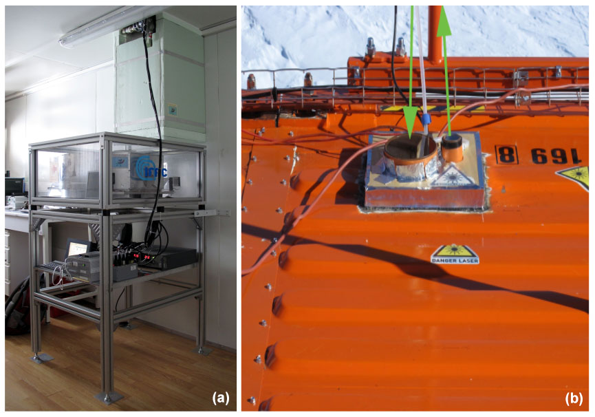
Figure 1 (a) REFIR-PAD Fourier transform spectroradiometer inside the PHYSICS shelter with the 1.5 m chimney connecting the instrument with the outside. (b) Output windows of the tropospheric lidar on the roof of the shelter.

The backscattering/depolarization tropospheric lidar is collocated inside the PHYSICS shelter. It was installed in 2008 and has operated in unattended mode, providing the backscattering and depolarization signal profiles with a temporal frequency of 10 min. The instrument uses the spectral channel at 532 nm of wavelength to provide the backscattering signal and the depolarization. Figure 1 shows the REFIR-PAD Fourier transform spectroradiometer inside the PHYSICS shelter and the aperture of the tropospheric lidar on the roof.

2.2 Micro rain radar (MRR)

The Micro Rain Radar-2 (MRR, Metek GmbH, Germany), a profiling Doppler radar, has been operating at Concordia station at Dome C since December 2018. It was installed on the roof of the PHYSICS shelter in a zenith-looking observation geometry and provides one measurement every minute. It operates at 24 GHz, measuring Doppler power spectra in 64 bins over 32 vertical range bins that were set to a width of 40 m. MRR has a compact design, being composed of a dish with a diameter of ∼ 60 cm and a small enclosure containing both a transmitting and a receiving apparatus. It is characterized by low power consumption and high robustness, making it suitable for deployment in remote regions for long-term unattended measurements. In fact, the MRR is a quite popular instrument for precipitation measurements in Antarctica in spite of the relatively low sensitivity (Bracci et al., 2022). The post-processing MRR procedure by Maahn and Kollias (2012) that partially improves the sensitivity of the system and removes spectra aliasing has been adopted.

An automatic data transfer system provides daily measurements directly to the storage server at the National Institute of Optics (CNR-INO) in Florence.

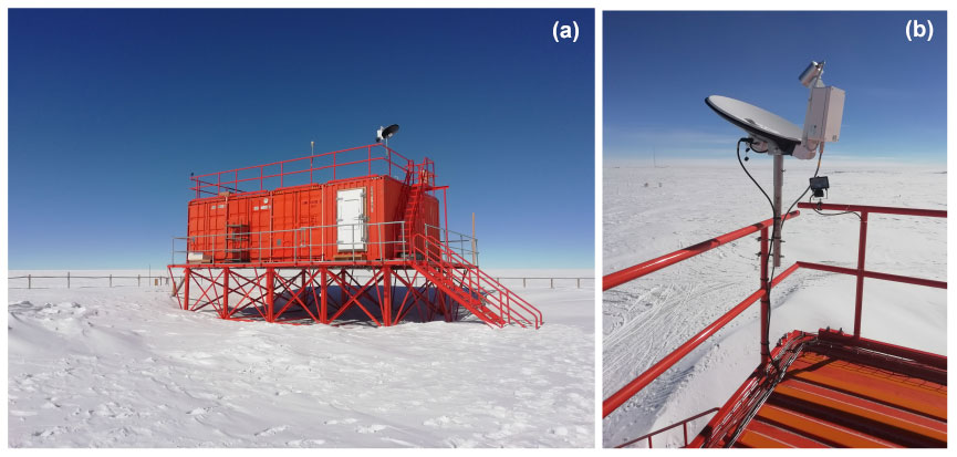
Figure 2 (a) PHYSICS shelter at Concordia station. (b) Micro rain radar (MRR) installed in 2018 on the roof of the shelter.

Figure 2 shows on the left side, the PHYSICS shelter at Concordia station, where REFIR-PAD spectroradiometer and the tropospheric lidar are installed; on the right side is the MRR, which is installed on the roof.

2.3 ICE- and HALO-CAMERA

The ICE-CAMERA (Del Guasta, 2022) is an optical imager mounted on the roof of the PHYSICS shelter. It is able to routinely image falling ice crystals by freezing them on a screen, rapidly photographing them, and then sublimating the deposited particles by heating the screen in a regular cycle. Sublimation of the ice particles occurs without melting on the ICE-CAMERA surface, as its temperature is kept below −5 ^∘C also during the heating of the plate.

The photographs are analyzed to sort and classify the precipitating ice crystals depending on their habit and sizes, and they are provided hourly except during maintenance or cleaning periods. A MATLAB software routine performs the automatic processing of the images: it subtracts the background, enlarges and reduces the binary image, deletes the edge objects, eliminates the single grains, creates and enlarges the grains bounding boxes, and finally sorts the grains depending on the increasing size for graphic use. In the last step, the software calculates the contour and the skeletonization of the remaining grains.

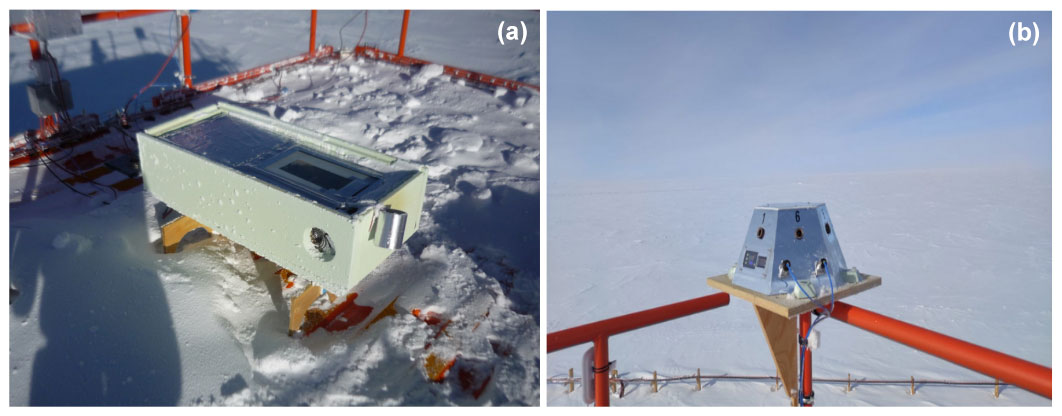
Figure 3 (a) ICE-CAMERA mounted on the roof of the PHYSICS shelter. (b) HALO-CAMERA installed on the handrail at the edge of the shelter.

HALO-CAMERA is a sky imager equipped with a sun tracker installed on the shelter roof used for monitoring the solar and lunar halos generated by the floating ice crystals. These halos occur because the scattering phase function at visible wavelengths for hexagonal ice crystals habits has two peaks at 22 and 46^∘ scattering angles. Figure 3 shows the two imagers deployed on the roof of the PHYSICS shelter at Concordia station.

In the work by Lawson et al. (2006), the images of ice crystals were recorded at the South Pole (Antarctica) by using two ground-based cloud particle imagers (CPIs) jointly with the LaMP (French Laboratoire de Meteorologie Physique) polar nephelometer, which measured the ice crystal phase function. In that work, it was found that the phase function showed the peak at 22^∘ when column-like and plate-like habits occur, but was smoother in case of rosette-like shape. We know that the presence of the peaks in the phase scattering function at visible wavelengths does not depend on the particular crystal habit but on the roughness of the crystal surface (Yang et al., 2013); the fact that Lawson et al. (2006) did not measure halos in the presence of bullet rosettes was probably related to a rougher crystal surface occurring during the formation of these particular crystals. In fact, as shown in Forster and Mayer (2022), the smooth crystal fraction (SCF) of the solid bullet rosettes tends to be at a minimum with respect to the other habits, that means the rough component is the most frequent. In summary, since plate-like crystals were not detected by the ICE-CAMERA during the precipitating event, we will use the evidence of halo formation as a good indicator of the occurrence of hexagonal ice columns in the Antarctic environment.

3 Methodology

The REFIR-PAD-retrieved cloud products were used to derive an estimation for the equivalent reflectivity Z_e, which can be compared with those obtained from MRR spectra. We used the cloud parameters, such as the ice optical depth (OD_i) at visible wavelengths and the ice effective diameter (D_ei), to derive the intercept (N_o) and the modal radius L_m of the particle size distribution (PSD). The PSD (denoted as n(L) in the formulas) was assumed as Γ-like distribution (Platnick et al., 2017; Matrosov et al., 1994; Turner, 2005) with exponent μ. The Γ size distribution is expressed as

$$\begin{array}{}\text{(1)}& n\left(L\right)=N_{\mathrm{o}}{L}^{\mathit{\mu }}{e}^{-(\mathrm{3}+\mathit{\mu })\frac{L}{L_{\mathrm{m}}}},\end{array}$$

where L is the length of assumed crystal in the given size bin and the mode is given by $\mathit{\mu }/(\mathrm{3}+\mathit{\mu })L_{\mathrm{m}}$. Then, we define the effective diameter following Yang et al. (2005):

$$\begin{array}{}\text{(2)}& D_{\mathrm{ei}}={\displaystyle \frac{\mathrm{3}}{\mathrm{2}}}{\displaystyle \frac{{\int }_{L_{min}}^{L_{max}}V\left(L\right)n\left(L\right)\mathrm{d}L}{{\int }_{L_{min}}^{L_{max}}A\left(L\right)n\left(L\right)\mathrm{d}L}},\end{array}$$

where V and A denote the particle volume and projected area, respectively. According to the measurements performed by Heymsfield et al. (2013, 2002) and the range of cloud temperature found at Dome C from our analysis, between −50 and −25 ^∘C, we assumed the μ coefficient of the PSD ranged between 0 and 2. With the effective diameter defined as in Eq. (2), the spectral radiance detected by REFIR-PAD turns out to be insensitive to the detailed shape of the size distribution (Wyser and Yang, 1998), in particular to the dispersion coefficient μ. We also verified this assertion by performing simulations of the downwelling spectral radiance for different values of D_e and optical depth by assuming different values of μ between 0 and 7 to generate the crystal infrared optical properties. Therefore, the results of the cloud properties retrieval are not affected by the choice of μ.

Once the PSD was defined, the effective MRR reflectivity was obtained by integrating the backscattering cross sections at 24 GHz (12.37 mm) tabulated in the database provided by Eriksson et al. (2018) over the PSD for different assumed crystal habits.

Figure 4 shows the backscattering and absorption cross sections contribution as a function of the particle length, L, for a normalized particle size distribution with L_m = 1000 µm. This value of L_m corresponds to an effective diameter D_e equal to 120 µm, as shown in Fig. 5. The case L_m = 1000 µm corresponds approximately to the average found from our retrieval analysis.

Figure 4 Left side: normalized PSD with L_m = 1000 µm (b) and the relative backscattering cross section at 24 GHz and absorption cross sections at 400 cm⁻¹ as a function of particle dimensions (a).

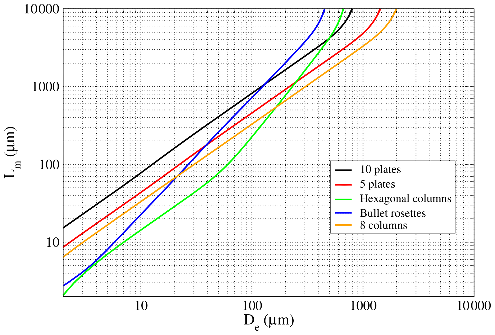
Figure 5 Relationship between the effective diameter (D_ei) and the modal radius (L_m) of the particle size distribution for the various ice crystal habits.

The results were obtained using the single particle optical properties of the large plate aggregates at 24 GHz for the backscattering and at 400 cm⁻¹ for the absorption cross sections. Figure 4 shows that the largest crystals of the assumed PSDs (Fig. 4b) provide the biggest contribution to the total backscattering cross section (representative of the MRR measurement) as shown in Fig. 4a. A similar result was obtained for the absorption cross section at 400 cm⁻¹ (assumed as the key parameter of the REFIR-PAD measurements at FIR), which, however, presents a peak slightly shifted towards the smaller dimensions (Fig. 4a). A considerable overlap between the two curves (mostly between 600–2000 µm) suggests that it was possible to obtain information on a large part of the PSD from FIR spectral measurements.

The MRR signal represents an indicator of the presence of large ice particles, while the infrared downwelling spectral radiance (R_ν) measured by REFIR-PAD shows more sensitivity to changes in smaller particles. In Fig. 6, we can see that the absolute values of the downwelling spectral radiance derivatives calculated with respect to D_ei for values of OD_i equal to 0.5 and 2 (upper and lower panels) at 400 cm⁻¹ (Fig. 6a and c) of wavenumber ν are more intense than at 830 cm⁻¹ (Fig. 6b and d), as much as 1 order of magnitude. The simulations were generated by placing an ice cloud close to the ground and the top at 5 km a.s.l., which was representative of the precipitating ice clouds we observed. From Fig. 6a and c, we can also notice that for D_ei larger than 100 µm, the derivatives calculated for the 10 plates aggregate habit shows the highest sensitivity. The color map of Fig. 7 shows that there is more sensitivity in the FIR region at 400 cm⁻¹ (Fig. 7a) for D_ei as high as about 300 µm and optical depth lower than 6, with respect to the mid-infrared at 830 cm⁻¹ (Fig. 7b). It is interesting that the bulk scattering properties of the 10 plates aggregate could be the suitable for retrieving atmospheric scenarios with large ice particles up to 300 µm for OD_i lower than 6.

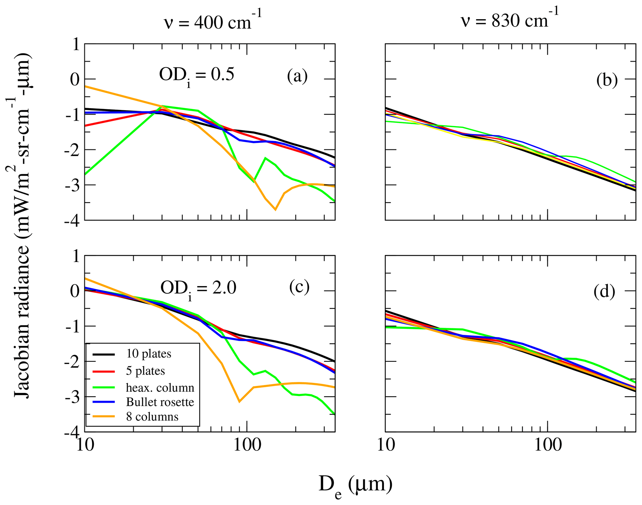
Figure 6 Absolute values of the downwelling spectral radiance derivatives with respect to the effective diameter simulated for two precipitating ice clouds with optical depth 0.5 (a, b) and two (c, d), at wavenumbers (ν) 400 cm⁻¹ (a, c) and 830 cm⁻¹ (b, d) for five different crystal habits.

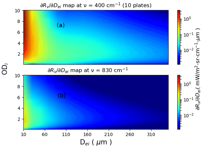
Figure 7 Color map of the same derivatives of Fig. 6, but only for the 10 plates aggregate and for multiple optical depth values ranging between 0.1 and 10.

In this work, we assumed that plate-like and droxtal-like crystals were not present, since at temperatures below −20 ^∘C, the prevalent regime is columnar because the ice supersaturation and the crystal growth rate are generally higher, as pointed out in Bailey and Hallett (2009). Moreover, at these temperatures, plates and droxtals show a low growth rate (Bailey and Hallett, 2009) and then have smaller sizes, below 60 and 100 µm, respectively (Yang et al., 2013; Lawson et al., 2006). Also, their occurrence is mostly found during diamond dust events and they were rarely observed in the ICE-CAMERA photographs during the precipitation events detected with the MRR. In the next section, we will show the low dependence on the habit type of the particle size distribution when the maximum crystal length stays in the range between 600 and 2000 µm. This peculiarity, and the fact that for the 10 plate aggregates, the downwelling spectral radiance is much more sensitive to the D_ei at the largest values above 100 µm with respect to the other habits, will be exploited to retrieve the effective diameter of the larger particles, as discussed in the next section.

The average absorption/extinction efficiencies (〈Q_a,ei〉_ν), the single scattering albedo (〈ω_i〉_ν), and the asymmetry factor (〈g_i〉_ν) at the wavenumber ν used to simulate the spectral radiances in the presence of ice clouds were calculated by assuming the PSD in Eq. (1). Thus, the 〈Q_a,ei〉_ν are given by the following (Yang et al., 2005):

$$\begin{array}{}\text{(3)}& {\displaystyle }{〈Q_{\mathrm{a},\mathrm{ei}}〉}_{\mathit{\nu }}={\displaystyle \frac{{\int }_{L_{min}}^{L_{max}}{Q}_{\mathrm{a},\mathrm{ei},\mathit{\nu }}\left(L\right)A\left(L\right)n\left(L\right)\mathrm{d}L}{{\int }_{L_{min}}^{L_{max}}A\left(L\right)n\left(L\right)\mathrm{d}L}}\text{(4)}& {\displaystyle }{〈g_i〉}_{\mathit{\nu }}={\displaystyle \frac{{\int }_{L_{min}}^{L_{max}}{g}_i\left(L\right)Q_{\mathrm{si},\mathit{\nu }}\left(L\right)A\left(L\right)n\left(L\right)\mathrm{d}L}{{\int }_{L_{min}}^{L_{max}}{Q}_{\mathrm{si},\mathit{\nu }}\left(L\right)A\left(L\right)n\left(L\right)\mathrm{d}L}}\text{(5)}& {\displaystyle }{〈{\mathit{\omega }}_i〉}_{\mathit{\nu }}=\mathrm{1}-{\displaystyle \frac{{〈Q_{\mathrm{ai}}〉}_{\mathit{\nu }}}{{〈Q_{\mathrm{ei}}〉}_{\mathit{\nu }}}},\end{array}$$

where $Q_{\mathrm{si},\mathit{\nu }}=Q_{\mathrm{ei},\mathit{\nu }}-Q_{\mathrm{ai},\mathit{\nu }}$ is the scattering efficiency, L_min and L_max denote the maximum length database limits equal to 2 and 10 000 µm, respectively, and A(L) is the projected area of the crystal.

3.1 Retrieval of the particle size distributions from REFIR-PAD spectral radiances

To simulate the downwelling spectral radiance of the atmosphere in the presence of ice clouds, the optical depth of the ice at the infrared wavenumbers was obtained through the following relationship (Yang et al., 2003a):

$$\begin{array}{}\text{(6)}& {\mathrm{OD}}_{i,\mathit{\nu }}={\displaystyle \frac{\mathrm{3}\cdot \mathrm{IWP}}{D_{\mathrm{ei}}{\mathit{\rho }}_{\mathrm{i}}}}{\displaystyle \frac{{〈Q_{\mathrm{ei}}〉}_{\mathit{\nu }}}{\mathrm{2}}}={\mathrm{OD}}_i{\displaystyle \frac{{〈Q_{\mathrm{ei}}〉}_{\mathit{\nu }}}{\mathrm{2}}},\end{array}$$

where ρ_i=917 kg m⁻³ is the ice density and 〈Q_ei〉_ν is the average extinction efficiency at the wavenumber ν. The optical coefficients as a function of L were taken from the database provided by Yang et al. (2013). From Eq. (6), by setting 〈Q_ei〉=2 since this factor can be assumed constant because of the large size parameters ($\frac{\mathit{\pi }{D}_{\mathrm{e}}}{\mathit{\lambda }}$), usually greater than 20 at the typical visible wavelengths, the OD_i was obtained as follows:

$$\begin{array}{}\text{(7)}& {\mathrm{OD}}_{\mathrm{i}}={\displaystyle \frac{\mathrm{3}\mathrm{IWP}}{{\mathit{\rho }}_{\mathrm{i}}{D}_{\mathrm{ei}}}}.\end{array}$$

Now we show that within the particle size range of MRR sensitivity, the PSD has in general a very low variability with respect to the crystal habit assumed in the range 600–2000 µm. The modal radius L_m of the PSD in Eq. (1) can be directly derived from the D_ei as shown on the left side of Fig. 5, while the intercept N_o can be obtained by using the expression of the ice water path (IWP) as follows:

$$\begin{array}{}\text{(8)}& \mathrm{IWP}=\mathrm{\Delta }z\cdot \mathrm{IWC}=\mathrm{\Delta }z\cdot {\mathit{\rho }}_{\mathrm{i}}\underset{L_{min}}{\overset{L_{max}}{\int }}V\left(L\right)n\left(L\right)\mathrm{d}L,\end{array}$$

with $\mathrm{\Delta }z=z_{\mathrm{t}}-z_{\mathrm{b}}$ the cloud thickness, the IWC denotes the average ice water content along the cloud layer, and z_t and z_b denote the cloud top and bottom heights (CTH, CBH), respectively, that were estimated from the lidar signal by applying the polar threshold (PT) algorithm (Van Tricht et al., 2014). Thus, replacing Eq. (1) in Eq. (8) and using Eq. (7) yields

$$\begin{array}{}\text{(9)}& N_{\mathrm{o}}\left(L_{\mathrm{m}}\right)={\displaystyle \frac{{\mathrm{OD}}_{\mathrm{i}}\cdot D_{\mathrm{ei}}}{\mathrm{3}\mathrm{\Delta }z\cdot C\left(L_{\mathrm{m}}\right)}},\end{array}$$

expressed in m⁻³ mm⁻⁸ and the volume factor C(L_m) is given by

$$\begin{array}{}\text{(10)}& C\left(L_{\mathrm{m}}\right)=\underset{L_{min}}{\overset{L_{max}}{\int }}V\left(L\right)L^{\mathrm{7}}{e}^{-\mathrm{10}\frac{L}{L_{\mathrm{m}}}}\mathrm{d}L,\end{array}$$

with V(L) defined as the volume of the crystals as a function of length as in Eq. (2). This result was obtained by assuming the optical depth and the effective diameter constant in the cloud in Eq. (9).

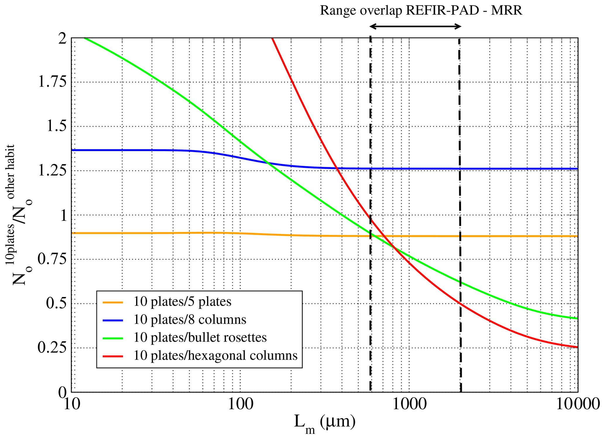
Figure 8 shows the curves of the ratio between the intercept (N_o) calculated from Eq. (9) for 10 plates aggregates with respect to those of the other habits of Figs. 6 and 5 as a function of L_m. Note that the range of L_m between about 600 and 2000 µm, where the sensitivity of REFIR-PAD and MRR mostly overlaps, represents the interval where the ratio is minimized, reaching a maximum deviation of about 50 % for the hexagonal columns.

Figure 8 Curves of the ratio between the intercept (N_o) calculated from Eq. (9) for 10 plates aggregates with respect to those of the other habits of Figs. 6 and 5 as a function of L_m.

The retrieval of the cloud properties was performed by using the Simultaneous Atmospheric and Cloud Retrieval (SACR) (Di Natale et al., 2020b), which is composed of a forward model (FM) and a retrieval code based on an optimal estimation (OE) approach. The downwelling spectral radiance was simulated in the spectral band between 200–980 cm⁻¹ (10–50 µm) through the FM as a function of the atmospheric profiles and the cloud parameters, such as the optical depth and the effective diameter. By using the entire band, we can retrieve a number of the atmospheric variables, since the infrared spectrum shows strong sensitivity to water vapor in the spectral region between 230–600 cm⁻¹ (16–43 µm), the temperature in the band centered at 667 cm⁻¹ (15 µm), the cloud optical depth in the atmospheric window between 820–980 cm⁻¹ (10–12 µm), and to the particle size below 600 cm⁻¹ (above 16 µm).

When liquid supercooled water exists overhead, the retrieval algorithm switches to the mixed-phase clouds retrieval (Di Natale et al., 2021; Turner et al., 2003), where the ice fraction (γ) was also retrieved together with the effective diameter of the water droplets (D_ew) in suspension. The ice fraction is defined as (Yang et al., 2003b):

$$\begin{array}{}\text{(11)}& \mathit{\gamma }={\displaystyle \frac{\mathrm{IWP}}{\mathrm{IWP}+\mathrm{LWP}}},\end{array}$$

where LWP is the liquid water path and, in case of only-ice phase, LWP=0 and γ was set to 1. In the presence of liquid content, D_ew was calculated as follows:

$$\begin{array}{}\text{(12)}& D_{\mathrm{ew}}=\mathrm{2}{\displaystyle \frac{{\int }_{R_{min}}^{R_{max}}{R}^{\mathrm{3}}n\left(R\right)\mathrm{d}R}{{\int }_{R_{min}}^{R_{max}}{R}^{\mathrm{2}}n\left(R\right)\mathrm{d}R}},\end{array}$$

where R is the radius of the droplets and the size distribution n(R) is still a Γ-function like for the ice. The liquid water optical depth (OD_w) was derived from Eq. (7) by using the parameters for water (LWP, D_ew) and the density ρ_w = 1000 kg m⁻³.

Since the profiles of water vapor and temperature were retrieved simultaneously with the cloud parameters, the final state vector used in the retrieval is given by (Di Natale et al., 2021) the following:

$$\begin{array}{}\text{(13)}& \mathit{x}=(D_{\mathrm{ei}},{\mathrm{OD}}_{\mathrm{i}},\mathit{U},\mathit{T},\mathrm{\Omega },\mathit{\beta }),\end{array}$$

for the only-ice case, and by defining the total optical depth OD = OD_i + OD_w, becomes

$$\begin{array}{}\text{(14)}& \mathit{x}=\left(D_{\mathrm{ei}},D_{\mathrm{ew}},\mathrm{OD},\mathit{\gamma },\mathit{U},\mathit{T},\mathrm{\Omega },\mathit{\beta }\right),\end{array}$$

for the case of mixed phase clouds, where U and T represent the vectors which contain the profile fitted levels of water vapor and temperature (7 for water vapor and 4 for temperature) at fixed pressure levels. Ω is the internal solid angle of the beam divergence which determines the formulation of the instrument line shape (ILS) and it was also fitted to take into account the effect of self-apodization. Finally, β is a scale factor on the frequency grid introduced to compensate for possible drift of the REFIR-PAD laser reference and for the shift due to the internal finite aperture (Bianchini et al., 2019; Di Natale et al., 2021).

SACR uses a Levenberg–Marquardt iterative algorithm to minimize the cost function (Rodgers, 2000) as follows:

$$\begin{array}{}\text{(15)}& \begin{array}{rl}{\mathit{\chi }}^{\mathrm{2}}& =(\mathit{y}-\mathrm{FM}(\mathit{x}\left){)}^T{\mathbf{S}}_y^{-\mathrm{1}}\right(\mathit{y}-\mathrm{FM}\left(\mathit{x}\right))\\ & +(\mathit{x}-{\mathit{x}}_{\mathrm{a}}{)}^T{\mathbf{S}}_{\mathrm{a}}^{-\mathrm{1}}(\mathit{x}-{\mathit{x}}_{\mathrm{a}}),\end{array}\end{array}$$

with y and x_a being vectors of the measurements and a priori parameters, respectively. S_y denotes the variance–covariance matrices (VCMs) of the measurements and contains the REFIR-PAD spectral noise, which is given by the square sum of the noise equivalent to signal ratio (NESR) and the calibration error (Bianchini et al., 2019). The NESR is calculated from the standard deviation of the four uncalibrated spectra provided during each REFIR-PAD measurement; the calibration error is due to the uncertainty on the temperature of the three black bodies (hot, cold, and reference) used for the radiance calibration procedure. The S_a matrix represents the VCM of the a priori errors associated to the a priori state vector x_a.

The a priori cloud parameters were set to large values equal to 100 µm for the effective diameters and 3 for the optical depth, with a priori error equal to 100 %, in order to avoid constraining the retrieval algorithm. We calculated the a priori thermodynamic profiles by interpolating those provided by the daily radiosondes launched at Concordia station routinely made by the Italian Meteo-Climatological Antarctic Observatory staff. We assumed an a priori error equal to 50 % for water vapor profiles and 1 % for temperature profiles with a correlation length equal to 2 km to regularize above 9 m of height (Di Natale et al., 2020a) and below 5 km. For heights above 5 km where sensitivity both to water vapor and temperature was very low and the information comes mainly from the a priori, a more stringent correlation length equal to 5 km was used to regularize the solution. Note that below 9 m, the levels of the a priori profiles were considered completely uncorrelated and the radiative contribution was mostly given by the temperature and humidity internal to the instrument.

The cost function in Eq. (15) is minimized through the OE and the Levenberg–Marquardt iterative formula given by

$$\begin{array}{}\text{(16)}& \begin{array}{rl}{\mathit{x}}_{i+\mathrm{1}}=& {\mathit{x}}_i+{\left[{\mathbf{K}}_{\mathrm{i}}^T{\mathbf{S}}_y^{-\mathrm{1}}{\mathbf{K}}_{\mathrm{i}}+{\mathit{\gamma }}_i{\mathbf{D}}_{\mathrm{i}}+{\mathbf{S}}_{\mathrm{a}}^{-\mathrm{1}}\right]}^{-\mathrm{1}}\\ & \left[{\mathbf{K}}_{\mathrm{i}}^T{\mathbf{S}}_y^{-\mathrm{1}}(\mathit{y}-\mathrm{FM}({\mathit{x}}_{\mathrm{i}}\left)\right)-{\mathbf{S}}_{\mathrm{a}}^{-\mathrm{1}}({\mathit{x}}_{\mathrm{i}}-{\mathit{x}}_{\mathrm{a}})\right],\end{array}\end{array}$$

where γ_i is the damping factor at the iteration i, K_i denotes the Jacobian matrix of FM, and D_i is a diagonal matrix as described in Di Natale et al. (2020b). The convergence is reached when variations on χ² are less than 1 ‰. The error of the retrieved parameters was obtained with the following relationship:

$$\begin{array}{}\text{(17)}& {\mathbf{S}}_x={\left({\mathbf{K}}^T{\mathbf{S}}_y^{-\mathrm{1}}\mathbf{K}+{\mathbf{S}}_{\mathrm{a}}^{-\mathrm{1}}\right)}^{-\mathrm{1}}.\end{array}$$

We considered the retrievals good unless there was a reduced ${\mathit{\chi }}_{\mathrm{red}}^{\mathrm{2}}=\frac{{\mathit{\chi }}^{\mathrm{2}}}{N-M}<\mathrm{3}$, with N number of spectral channels used and M number of retrieved parameters, as in Di Natale et al. (2020a).

The results of Fig. 9 show, as similarly done in Maestri et al. (2019), the retrievals performed with the different habits averaging the differences between the REFIR-PAD radiances and the simulated spectra in 28 microwindows reported in Turner et al. (2003), chosen between 360 and 970 cm⁻¹. We found that the aggregates of 10 plates show the best agreement with the measurements, with the lowest ${\mathit{\chi }}_{\mathrm{red}}^{\mathrm{2}}$.

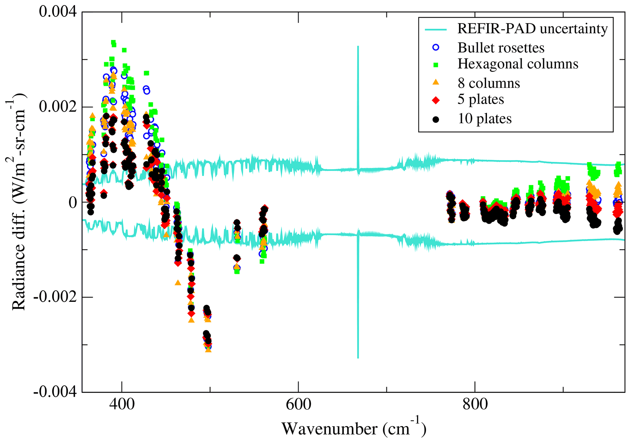
Figure 9 Comparison with respect of the averaged REFIR-PAD instrumental uncertainty (turquoise curves) of the mean differences between the measurements and the simulated spectra calculated in 28 selected microwindows reported in (Turner et al., 2003) for various ice crystal habits.

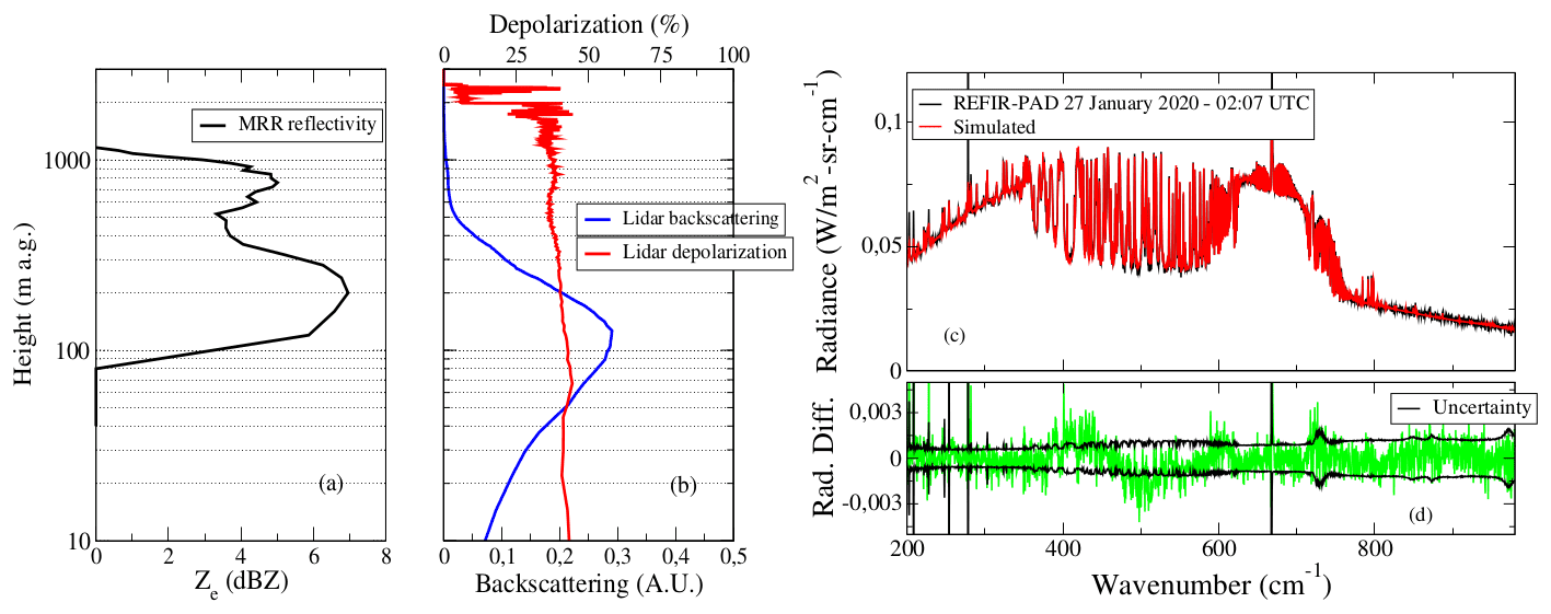
Figure 10 (a) Reflectivity profiles provided by the MRR on the day 27 January 2020 at 02:07 UTC. (b) Backscattering (blue curve) and depolarization (red curve) lidar profiles. (c) Comparison of a REFIR-PAD measurement (black curve) at 08:24 UTC on 10 December 2020 with the simulated spectra at the last iteration (red curve). (d) Comparison of the differences between the measured and the simulated spectrum (green curve) with the instrumental noise (black curve).

Figure 10a and b show an example of the measurement of vertical reflectivity provided by the MRR on 27 January 2020 at 02:07 UTC, together with the lidar and REFIR-PAD measurements. The middle panel shows the lidar backscattering signal in arbitrary units (blue curve) and the depolarization (red curve). When the depolarization was higher than 15 %, the cloud was classified as ice cloud as described in Cossich et al. (2021). Figure 10c reports the REFIR-PAD measurement (black curve) in comparison with the simulated spectrum (red curve); Fig. 10d shows the differences (green) in comparison with the instrumental uncertainty (black). The plot shows a very good agreement between the measurement and the simulation; the retrieval provides $D_{\mathrm{ei}}=(\mathrm{121}\pm \mathrm{4})$ µm, $L_{\mathrm{m}}=(\mathrm{994}\pm \mathrm{33})$ µm, OD${}_{\mathrm{i}}=(\mathrm{1.270}\pm \mathrm{0.004})$, and ${\mathit{\chi }}_{\mathrm{red}}^{\mathrm{2}}$=1.3.

A direct retrieval of the optical extinction or ice fraction from the lidar measurements was not possible due to the high noise of the signal above the cloud top heights, which does not allow the application of a retrieval algorithm such as the Klett method. These lidar measurements represent qualitative data, which allow identifying the occurrence of clouds and assessing their position and the presence of ice and supercooled water.

4 Results and discussion

Figure 11 shows the scatterplots of the OD_i−D_ei retrieved from REFIR-PAD (black circles). From these parameters, L_m and N_o were obtained and they allowed to obtain the PSD from Eq. (1), which was used to derive the effective reflectivity Z_e at 24 GHz for the comparison with the MRR: the green circles in Fig. 11 denote the points detected by the MRR with reflectivity higher than −5 dBZ. We can see that D_ei retrieved with REFIR-PAD mostly ranged between 20–250 µm, but those detected also by the MRR stayed above 70 µm.

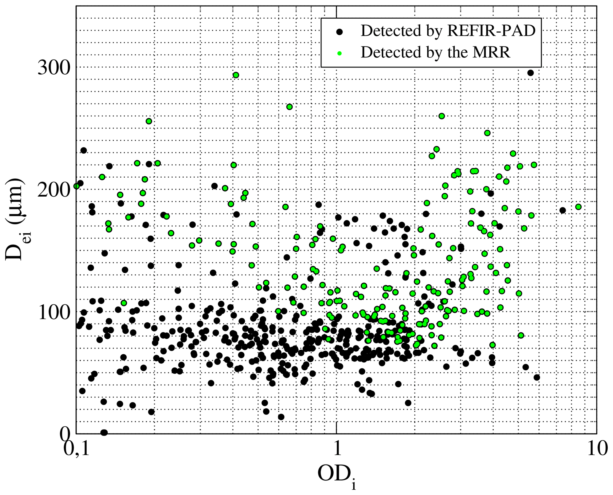
Figure 11 Variability of the retrieved ice optical depth (OD_i) as a function od the effective diameter (D_ei). The green circles denote the values detected also by the MRR.

The retrieved ODs from REFIR-PAD spectra over all the analyzed data spanned mostly in the broad range between 0.1 and 5, as we can see from Fig. 11. In Fig. 12, the variability in the REFIR-PAD spectra during the day of 23 July 2019 is shown.

Figure 12 Variability of the cloudy spectra detected by REFIR-PAD during the day of 23 July 2019.

The average crystal length can be calculated through the retrieved PSD as

$$\begin{array}{}\text{(18)}& L_{\mathrm{av}}^{\mathrm{REFIR}}={\displaystyle \frac{{\int }_{L_{min}}^{L_{max}}L\cdot n\left(L\right)\mathrm{d}L}{{\int }_{L_{min}}^{L_{max}}n\left(L\right)\mathrm{d}L}}.\end{array}$$

This value was used for the comparison with the crystal size estimated from the ICE-CAMERA measurements. The uncertainty was calculated by propagating the retrieval error in Eq. (18) and the one coming from the error in evaluating the CTH with the PT algorithm, which can be as large as 500 m in the worst cases. The CBH was considered not affected by error since it was always very close to the ground because we were treating precipitating events. If we indicate the following:

$$\begin{array}{}\text{(19)}& f_{l+\mathrm{1},\mathit{\mu }}\left(L_{\mathrm{m}}\right)=\underset{L_{min}}{\overset{L_{max}}{\int }}{L}^{\mathit{\mu }+l}{e}^{-(\mathit{\mu }+\mathrm{3})\frac{L}{L_{\mathrm{m}}}}\mathrm{d}L\mathrm{with}l=\mathrm{0},\mathrm{1},\end{array}$$

the uncertainty $\mathrm{\Delta }{L}_{\mathrm{av}}^{\mathrm{REFIR},\mathrm{ret}}$ due to the retrieval error turns out to be

$$\begin{array}{}\text{(20)}& \mathrm{\Delta }{L}_{\mathrm{av},\mathit{\mu }}^{\mathrm{REFIR}}=\sqrt{{\left|{\displaystyle \frac{\partial L_{\mathrm{av}}^{\mathrm{REFIR},\mathrm{ret}}}{\partial f_{\mathrm{1},\mathit{\mu }}}}\right|}^{\mathrm{2}}\mathrm{\Delta }{f}_{\mathrm{1},\mathit{\mu }}^{\mathrm{2}}+{\left|{\displaystyle \frac{\partial L_{\mathrm{av}}^{\mathrm{REFIR}}}{\partial f_{\mathrm{2},\mathit{\mu }}}}\right|}^{\mathrm{2}}\mathrm{\Delta }{f}_{\mathrm{2},\mathit{\mu }}^{\mathrm{2}}},\end{array}$$

with

$$\begin{array}{}\text{(21)}& \begin{array}{rl}& \mathrm{\Delta }{f}_{l+\mathrm{1},\mathit{\mu }}={\displaystyle \frac{\mathrm{10}\mathrm{\Delta }{L}_{\mathrm{m}}}{L_{\mathrm{m}}^{\mathrm{2}}}}\underset{L_{min}}{\overset{L_{max}}{\int }}{L}^{\mathit{\mu }+\mathrm{1}+l}{e}^{-(\mathit{\mu }+\mathrm{3})\frac{L}{L_{\mathrm{m}}}}\mathrm{d}L\\ & \mathrm{with}l=\mathrm{0},\mathrm{1},\end{array}\end{array}$$

where ΔL_m denotes the retrieval error of L_m.

The uncertainty $\mathrm{\Delta }{L}_{\mathrm{av}}^{\mathrm{REFIR},\mathrm{CTH}}$ due to the CTH error was calculated by repeating the retrieval for each measurement increasing and decreasing this latter by 500 m; the maximum deviation from the original value of $L_{\mathrm{av}}^{\mathrm{REFIR}}$ was considered its associated uncertainty. The total uncertainty was finally calculated as follows:

$$\begin{array}{}\text{(22)}& \mathrm{\Delta }{L}_{\mathrm{av},\mathit{\mu }}^{\mathrm{REFIR}}=\sqrt{{\left|\mathrm{\Delta }{L}_{\mathrm{av},\mathit{\mu }}^{\mathrm{REFIR}}\right|}^{\mathrm{2}}+{\left|\mathrm{\Delta }{L}_{\mathrm{av}}^{\mathrm{REFIR},\mathrm{CTH}}\right|}^{\mathrm{2}}},\end{array}$$

where $\mathit{\mu }=\mathrm{0},\mathrm{1},\mathrm{2}$ in our analysis.

4.1 Derivation of the equivalent radar reflectivity at 24 GHz

We can calculate the effective reflectivity at the MRR wavelength λ = 12.37 mm (24 GHz) by using the PSD retrieved from REFIR-PAD in the following formula (Eriksson et al., 2018; Tinel et al., 2005):

$$\begin{array}{}\text{(23)}& Z_{\mathrm{e}}^{\mathrm{REFIR}}={\displaystyle \frac{{\mathit{\lambda }}^{\mathrm{4}}}{{\mathit{\pi }}^{\mathrm{5}}{K}_{\mathrm{w}}^{\mathrm{2}}}}\underset{L_{min}}{\overset{L_{max}}{\int }}{\mathit{\sigma }}_{\mathit{\lambda },h}(L,T_{\mathrm{cld}})n\left(L\right)\mathrm{d}L,\end{array}$$

where $K_{\mathrm{w}}^{\mathrm{2}}$ = 0.92 is the dielectric constant of water and ${\mathit{\sigma }}_{\mathit{\lambda },h}(L,T_{\mathrm{cld}})$ is the backscattering cross section in m² for the habit h at wavelength λ, T_cld in K is the cloud temperature, and L in mm as provided by the Eriksson et al. (2018) microwaves scattering database, which we name for simplicity EMD (Eriksson microwave database). We set L_max equal to 10 mm as for the FIR properties and Z_e is expressed in mm⁶ m⁻³.

The backscattering cross sections are tabulated for 34 different habits, including liquid spheres and spherical graupel, and 17 of them are classified as single crystals, 3 habits represent heavily rimed particles, and the remaining habits are aggregates of different types, including snow and hail. Even though the particle sizes vary considerably among the habits, and the maximum length of 10 and 20 mm are typical values for the largest single crystal and aggregate particles, respectively, we limited the integral in Eq. (23) up to a cut-off value equal to 10 mm, corresponding to the maximum crystal length of the Yang et al. (2013) FIR database. The EMD is compiled with a broad coverage in frequency (1–886 GHz) for three values of temperature (190, 230 and 270 K), so that the final value can be obtained by interpolating. The temperature T_cld was calculated from the temperature profiles retrieved with SACR and the bounding heights CBH and CTH of the precipitating clouds.

The Z_e measured by the MRR was averaged along the vertical path to provide a parameter to compare with those retrieved from REFIR-PAD observations, which in turn represents an average over the cloud thickness as

$$\begin{array}{}\text{(24)}& Z_{\mathrm{e}}^{\mathrm{MRR}}={\displaystyle \frac{{\int }_{z_{\mathrm{b}}}^{z_{\mathrm{t}}}{Z}_{\mathrm{e}}\left(z\right)\mathrm{d}z}{\mathrm{\Delta }z}},\end{array}$$

where z is the height.

Only MRR Z_e values above −5 dBZ were analyzed and included in the analysis, since below this value the results were not considered sufficiently reliable (Maahn and Kollias, 2012; Souverijns et al., 2017). Figure 13a reports the reduced ${\mathit{\chi }}_{\mathrm{red}}^{\mathrm{2}}$ obtained from the Z_e retrieved from REFIR-PAD and those measured by the MRR by assuming μ = 0,1,2 (green, blue, red curves) and considering their respective retrieval errors; Figure 13b shows the total number of measurements (N) available considering the cut-off at −5 dBZ. On the x axis, we reported the habit index explained in Table 1. Habits were selected based on the criteria of having the ${\mathit{\chi }}_{\mathrm{red}}^{\mathrm{2}}$ close to 1 and maximize the number of measurements by assuming some thresholds (dashed black lines in Fig. 13). Further requirements were that N had to be greater than 25 and ${\mathit{\chi }}_{\mathrm{red}}^{\mathrm{2}}$ had to stay between 0.5 and 2, since when it decreases too much, it usually indicates that the error is overestimated. The selected cases that complied with the criteria were identified with cyan triangles. From Fig. 13 it is noted that there is little difference by varying μ in the range 0–2 for the selected cases, so that we assumed an average value μ = 1 for the ensuing analysis.

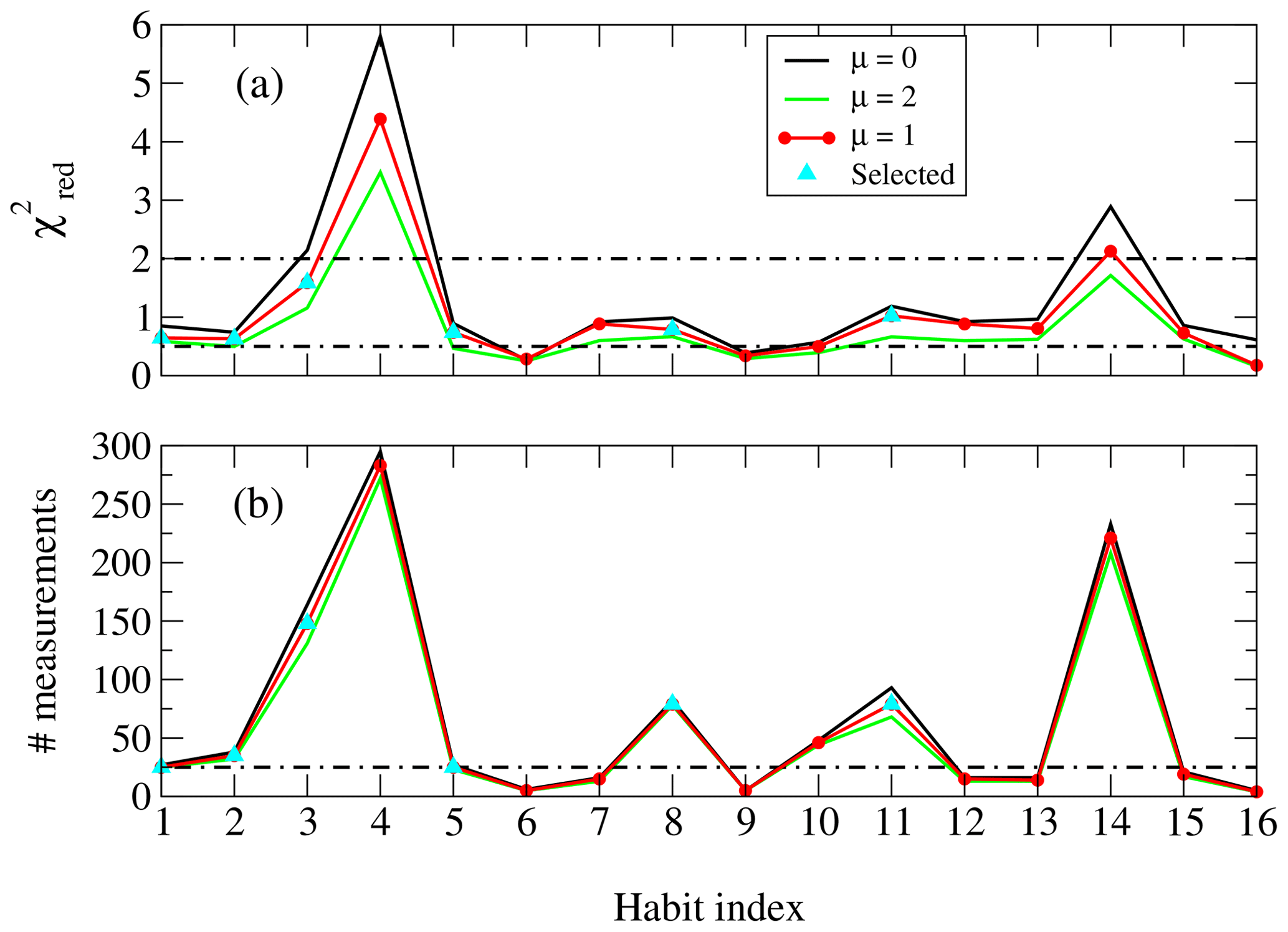
Figure 13 (a) Reduced ${\mathit{\chi }}_{\mathrm{red}}^{\mathrm{2}}$ calculated from the Z_e retrieved from REFIR-PAD and those measured by the MRR by assuming μ = 0, 1, 2 , blue, red curves). (b) Number of measurements above the −5 dBZ threshold assumed for the analysis.

Eriksson et al. (2018)

Table 1 Crystal habits used from Eriksson et al. (2018) database and their corresponding index in Fig. 13.

The habits that led to best accordance with the radar measurements were the $\mathrm{5}/\mathrm{6}$ branches bullet rosettes, the thin and long columns, and the 8-columns/large block aggregates. Figure 14 shows the comparison of the MRR measured reflectivities with those obtained from REFIR-PAD by using some of the habits from EMD in Table 1 that provided the best agreement. The high occurrence of hexagonal columns, aggregates, and bullet rosettes was confirmed by the ICE-CAMERA photographs. In particular, the high occurrence of hexagonal columns was corroborated by the presence of 22^∘ halos detected by the co-located HALO-CAMERA sky images as shown in previous studies at South Pole by Lawson et al. (2006). It also should be noted that while the correlation coefficient turned out to be moderate (maximum ∼ 0.3), this was mostly due to the difficulty of retrieving with good accuracy the shape of the PSD from the FIR observations, and in particular the intercept N_o, for large particle sizes. This shows the need to increase the number of measurements for improving the statistical distribution. However, the results indicate that in the particle size range between about 600 and 2000 µm, the retrieval algorithm was able to estimate the intercept assuming the dispersion coefficient μ in the range 0–2, as shown in Fig. 14. The distributions of the retrieved N_o converted in cm⁻⁵ and the slope $\mathrm{\Lambda }=(\mathrm{3}+\mathit{\mu })/L_{\mathrm{m}}$ in cm⁻¹ as a function of the retrieved cloud temperature (T_cld) were found in very good accordance with those found in Heymsfield et al. (2013, 2002) and Wolf et al. (2019), and they were shown in Fig. 15, panels a and b, respectively. Note that N_o varied mostly between 10⁻²–10⁴ cm⁻⁵, while Λ mostly between 20–200 cm⁻¹. The average relative error found for N_o was equal to 20 %, which was comparable to the systematic error due to the assumption of a specific habit in the retrieval as shown in Fig. 8.

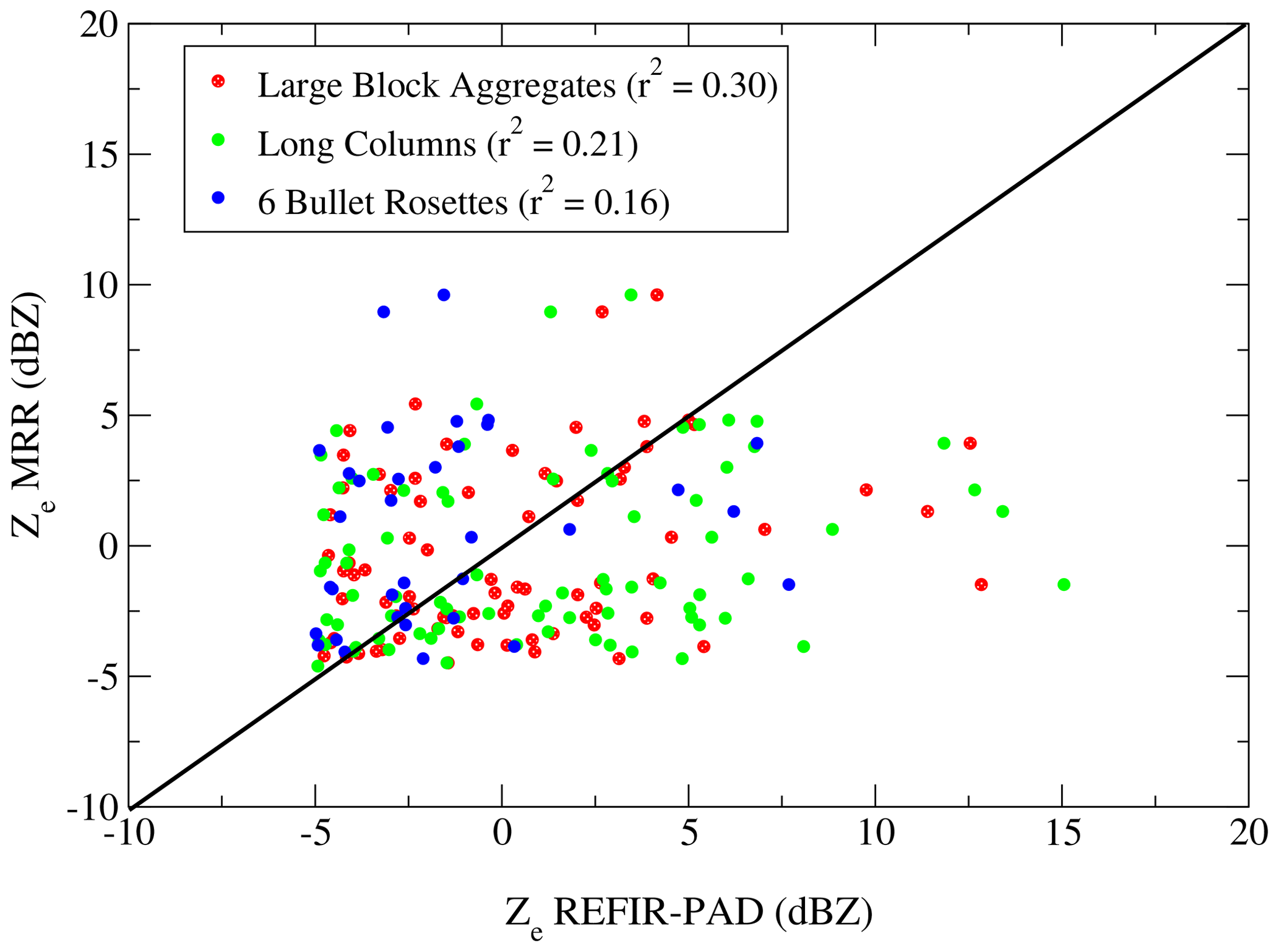
Figure 14 Scatterplots of the Z_e measured by the MRR and those retrieved from REFIR-PAD by assuming μ = 1 and by using the habits from Eriksson et al. (2018) database that provided the best accordance: long columns, large plates aggregates, and 6 branches bullet rosettes.

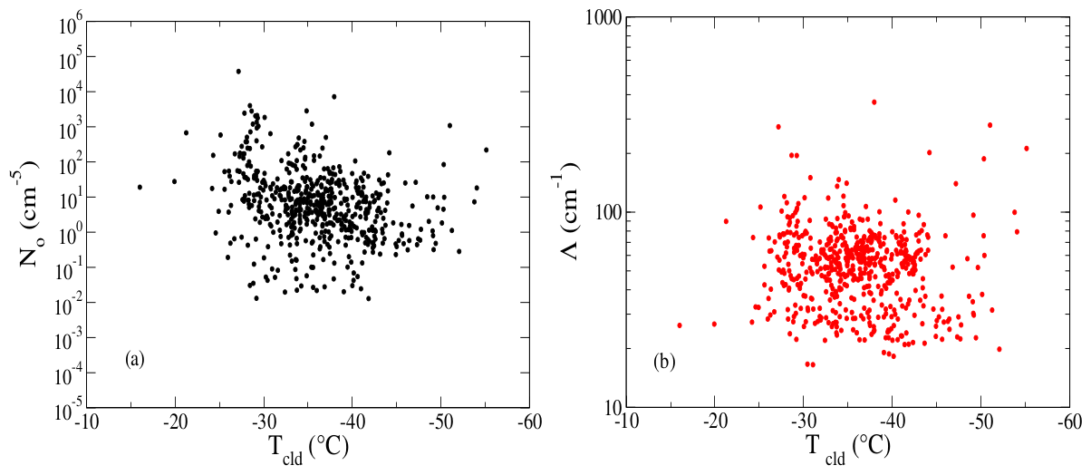
Figure 15 (a, b) Intercept N_o and slope Λ as a function of the cloud retrieved temperature (T_cld).

4.2 Assessment of particle size and habit from ICE- and HALO-CAMERA

An average length of the ice crystals falling on the ICE-CAMERA screen can be defined by the area of the bounding box (A_box) containing the crystal itself, as shown in Figs. 20 and 25 (red boxes). This parameter represents the diameter of the crystal with the projected area equal to the bounding box and it was calculated in µm (1 image pixel = 7 µm) by averaging over all of the acquired crystals at the ith scanning through the following formula:

$$\begin{array}{}\text{(25)}& L_{\mathrm{av}}^{\text{ICE-CAMERA}}={\displaystyle \frac{\mathrm{14}}{N_{\mathrm{c}}}}\sum _{i=\mathrm{1}}^{N_{\mathrm{c}}}\sqrt{{\displaystyle \frac{A_{\mathrm{box},i}}{\mathit{\pi }}}},\end{array}$$

where N_c is the number of crystals acquired at the ith scanning. The corresponding uncertainty is given by

$$\begin{array}{}\text{(26)}& \mathrm{\Delta }{L}_{\mathrm{av}}^{\text{ICE-CAMERA}}={\displaystyle \frac{\mathrm{7}\mathrm{\Delta }{A}_{\mathrm{box}}}{N_{\mathrm{c}}\sqrt{\mathit{\pi }}}}\sqrt{\sum _{i=\mathrm{1}}^{N_{\mathrm{c}}}{\displaystyle \frac{\mathrm{1}}{A_{\mathrm{box},i}}}},\end{array}$$

where $\mathrm{\Delta }{A}_{\mathrm{box}}=\mathrm{\Delta }{A}_{\mathrm{box},i}\simeq \mathrm{5}$ pixel ∀i is the uncertainty in pixel associated to each bounding box.

4.3 Selected days for case studies

We selected 4 d in 2020 among all analyzed data, specifically 23/24 February and 21/24 April, when most of the measurements from the different instruments were simultaneously available. From the retrieved temperature profiles, we assessed the average in-cloud temperatures by weighting the profiles with the corresponding backscattering lidar signal. The temperature varied between −20 and −40 ^∘C and on average was found to be −28 ^∘C. Specifically for the cases discussed hereafter, the average temperatures were about −30 ^∘C during the days of 23 February, 24 February, and 23 April, while during the day of 21 April, temperatures were about −25 ^∘C.

Figure 16 shows four retrieved temperature profiles (colored lines on Fig. 16a) for the dates reported in the label. Note the inversion in the temperature profile typical of the Antarctic Plateau at around 750 m above the ground. The ground peak corresponds to the internal temperature of the instrument, since it was treated as a separated environment in the retrieval procedure as already mentioned. On 21 April 2020, the inversion of the temperature reached −6 ^∘C at around 1000 m. In Fig. 16b, we have also reported the backscattering lidar profiles which show that the precipitating clouds occurred for these cases below 500 m.

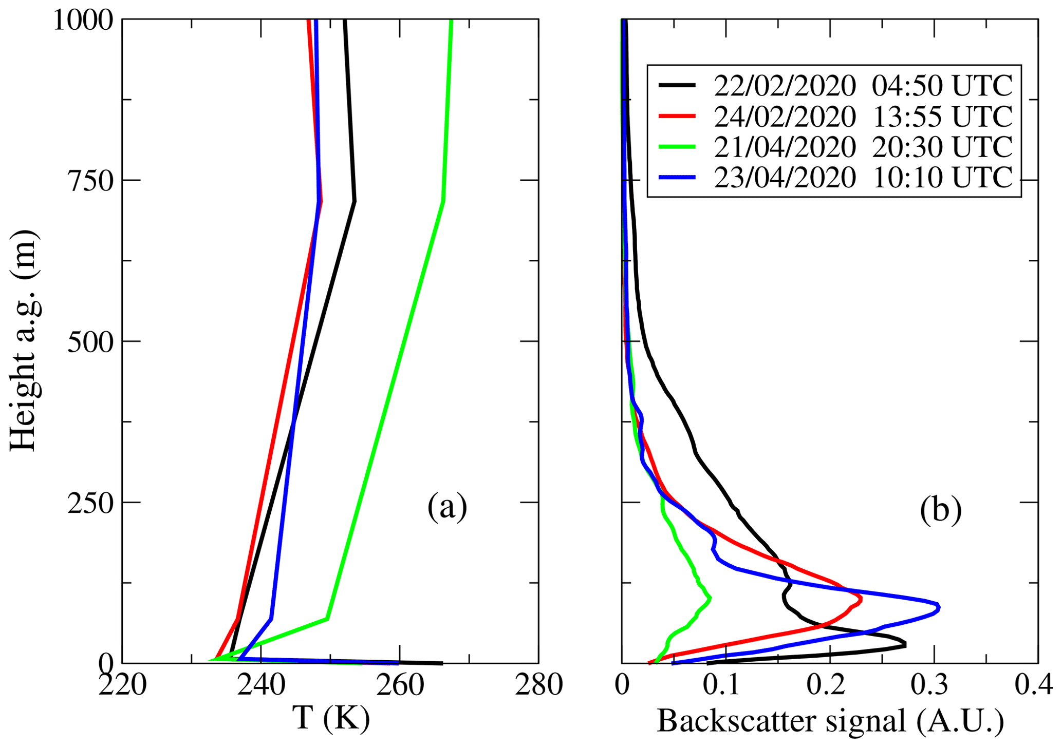
Figure 16 (a) Retrieved temperature profiles during the selected days of measurement. (b) Backscattering lidar signal in arbitrary units for the analyzed measurements.

4.3.1 Days of 23 and 24 February 2020

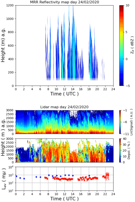
The MRR reflectivity time–height cross-section for the selected days of 23 and 24 February 2020 are shown on the upper panel of Fig. 17. The data were not continuous because of the filtering procedure due to the sensitivity of the MRR to the largest particles. The corresponding color map of the backscattering and depolarization lidar signals are also shown on the right of Fig. 17. The depolarization lidar shows that precipitation starts from the passage of ice clouds between 02:00–04:00 UTC, when larger ice crystals formed as detected by the MRR signal, which reached a few dBZ above 0. Then the precipitation continued but with particles decreasing in size; in fact, the MRR signal decreases rapidly. On 24 February, an intense precipitation started at 07:00 UTC and finished at about 22:00 UTC; this was composed of larger crystals as clear from the MRR signal in the upper panel of Fig. 18. In particular, the signal reached about 3 dBZ at 11:30, 14:30, and 18:30 UTC. Figure 18 also shows the comparison of the average crystal length (L_av) retrieved from REFIR-PAD infrared spectra (red diamonds) with those obtained from the ICE-CAMERA (blue dots). Continuous MRR measurements and ICE-CAMERA data were available most of the time on both days, as shown in Fig. 17.

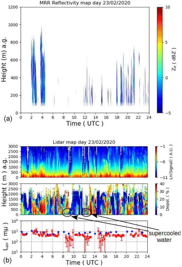
Figure 17 (a) Vertical profiles of reflectivity Z_e in dBZ obtained by the MRR as a function of the UTC time in hours of the day of 23 February 2020. (b) In the upper and middle panels is the backscattering and depolarization signals detected by the tropospheric lidar and in the lower panel the comparison of the average crystals length of the ice crystals (L_av) retrieved from REFIR-PAD spectra (red diamonds) with those estimated from the ICE-CAMERA (blue dots).

Figure 18 As in Fig. 17, but for the dayof 24 February 2020.

Mixed-phase clouds passed above the site on 23 February between 08:00–09:00 and 12:00–13:00 UTC, when their occurrence was detected by the lidar depolarization signal at around 200 m above the ground (indicated with black arrows) and, in particular, the supercooled liquid water formed layers of 100 and 300 m of thickness on the 23 and 24 February, respectively. The average retrieved precipitable water vapor (PWV) was found equal to 1.33 and 0.98 mm on the days 23 and 24 February, respectively, with average cloud temperatures of about −40 and −39 ^∘C. The average temperature of the water layers was found equal to −31 ^∘C.

In the first mixed-phase cloud time slot, the retrieval provided an average ice fraction γ equal to 0.47 with LWP equal to 0.62 g m⁻², while in the second time slot, values were found equal to 0.56 and 1.5  g m⁻².

The lower panels in Figs. 17 and 18 indicate that the values of the average crystal lengths retrieved from REFIR-PAD and those estimated from ICE-CAMERA varied between 700–1200 and 700–1000 µm, respectively, and they were mostly in very good agreement for most of the cases, particularly on 23 February.

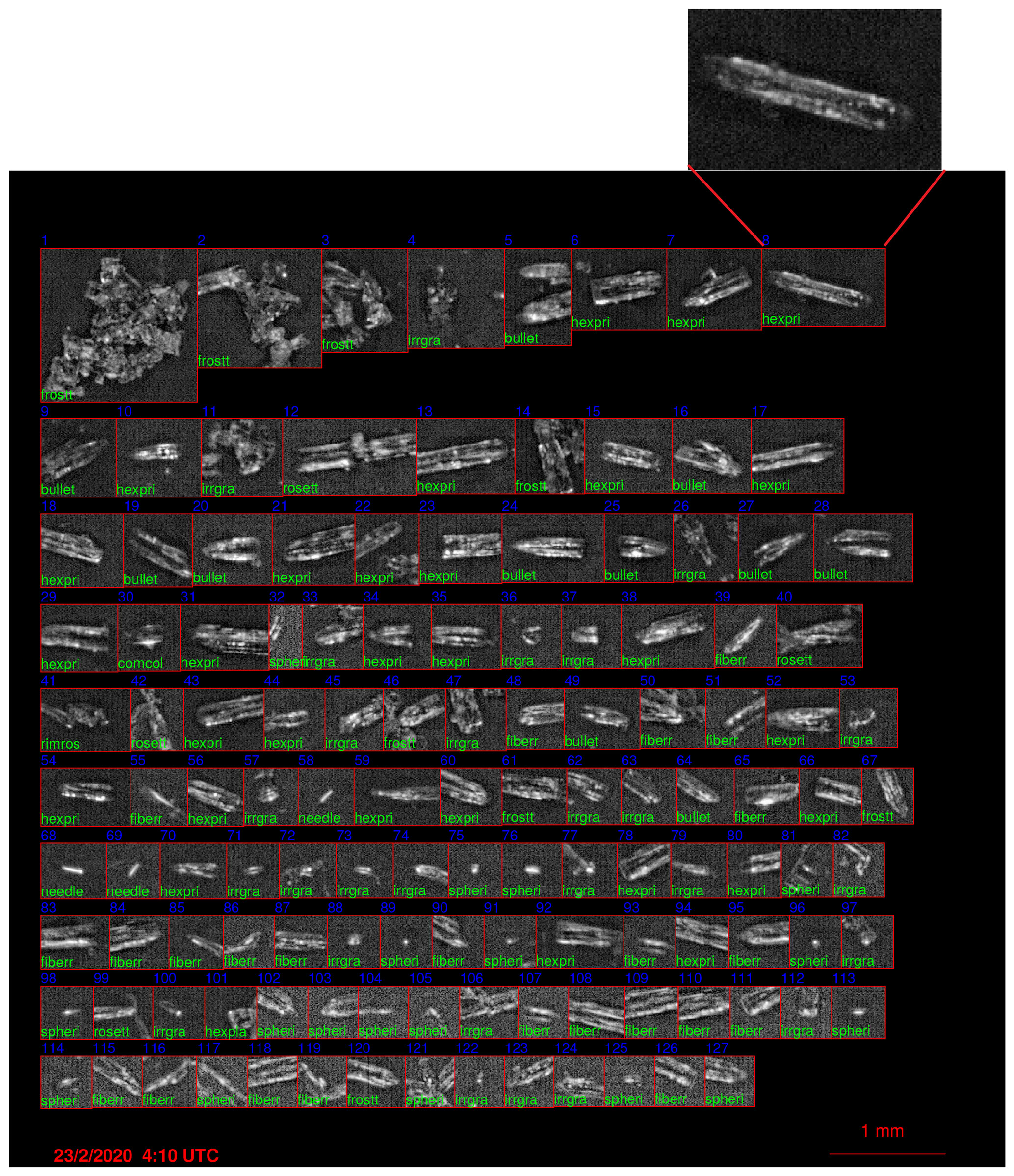
Figure 19 ICE-CAMERA photographs for the day of 23 February at 04:10 UTC. The photograph indicates the presence of mostly hexagonal columns. In the upper part is the zoom of a single column crystal.

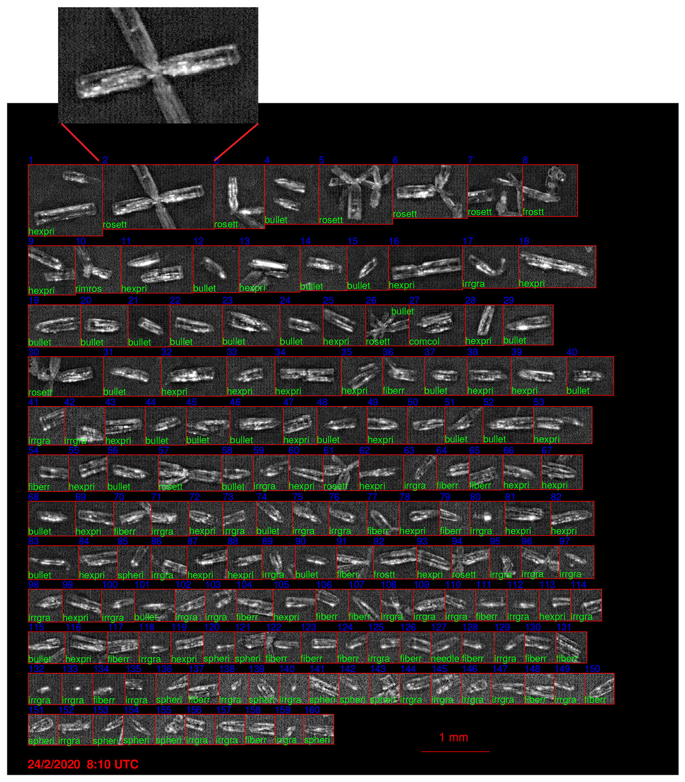
Figure 20 As Fig. 19, but for the day of 24 February 2020 at 08:10 UTC. The photograph indicates a large amount of hexagonal columns with a small amount of bullet rosettes also present. In the upper part is the zoom of a single bullet rosette crystal.

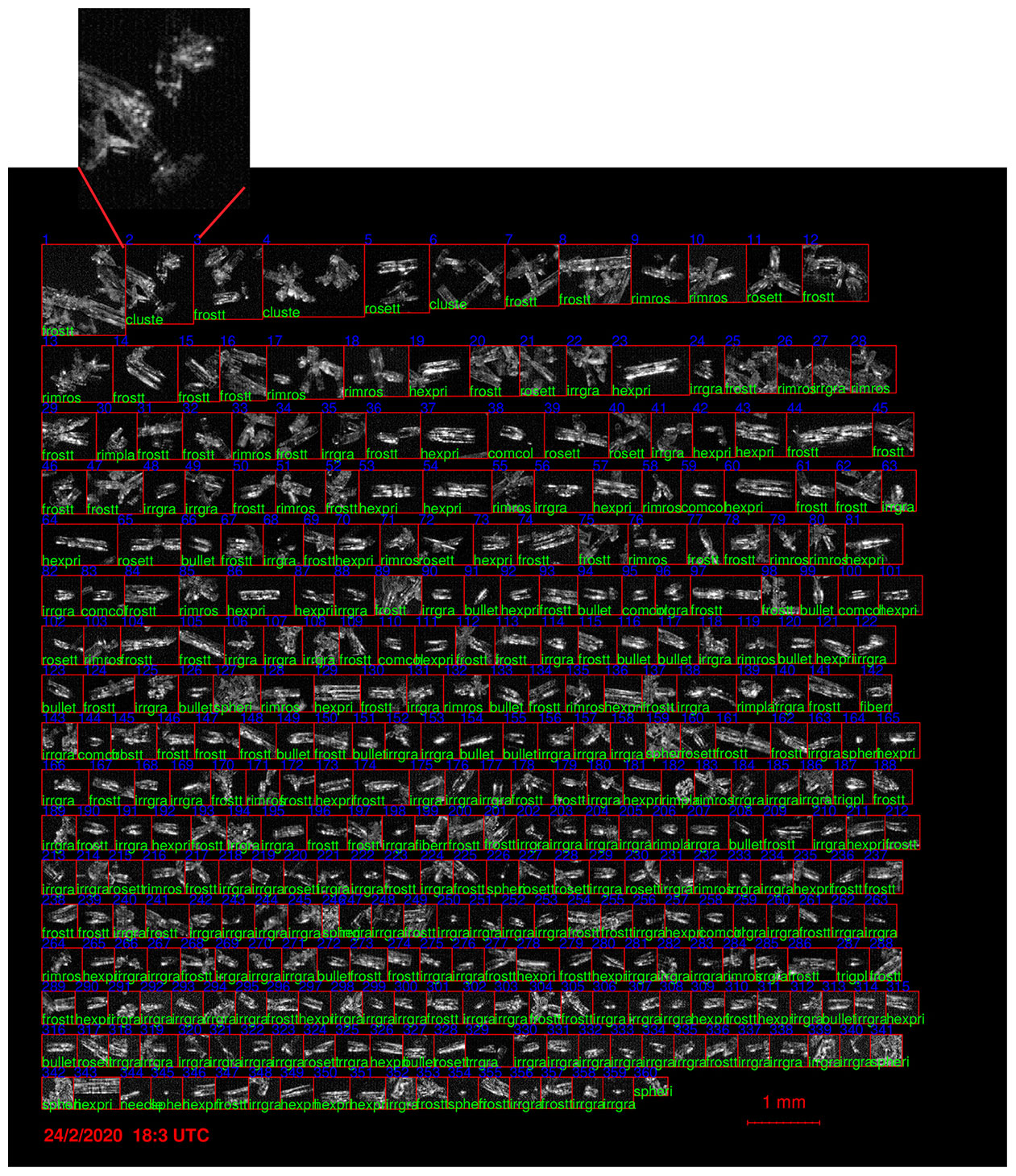
Figure 21 As Fig. 20 still for the day of 24 February 2020, but at 18:03 UTC. The photograph indicates a large amount of hexagonal columns and aggregates (or cluster) with a small amount of rimmed rosettes. In the upper part is the zoom of an aggregate.

Figures 19 and 20 show the photographs taken by the ICE-CAMERA at 04:10 and 08:10 UTC on the days of 23 and 24 February 2020, respectively. These times were selected because were close to the strong precipitation that occurred at those times detected both by the lidar and the radar, as we can note from Figs. 17 and 18, when the sunlight generated the halos. Figure 21 also shows the photograph at 18:03 UTC on 24 February, right before the intense precipitation detected by the lidar and radar (Fig. 18), where one can note the presence of columnar aggregates (or clusters) and rimmed rosettes beside the hexagonal columns. The crystal habits were automatically cataloged by the internal algorithm and labeled with the green labels. The solid column particles are represented by hexagonal columns (label: hexpri) or bullet (label bullet), which are columns with a tip at one end; aggregates (irrgra, clusters) were also found, together with bullet rosettes (rosette) or rimed rosettes (rimros). In general, some elements needed to be discarded since they represent volatile material (label: fiberr) produced by the main building of the station.

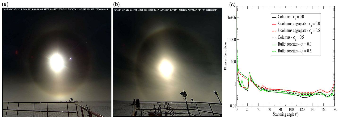
Figure 22 HALO-CAMERA images for the days of 23 (a) and 24 (b) February 2020. On panel (c), the simulated phase functions at 532 nm for the three habits considered with roughness σ_r = 0 (smooth crystal surface) and σ_r = 0.5 (severe rough crystal surface).

Ice crystals shown in Fig. 19 on the day of 23 February indicate that almost only column-like crystals were present. On the contrary, the photograph in Fig. 20 on the day of 24 February indicates the presence of bullet rosettes. The prevalence of hexagonal columns was confirmed by the detection of solar halos in the HALO-CAMERA images at the same times, as shown in Fig. 22 for both days. In fact, the right panel shows that the phase functions of the smooth columns, aggregate, and bullet rosettes (σ_r=0) present a strong scattering peak at 22^∘, which is responsible for the most intense halos, while for the roughest particles (σ_r=0.50), the function is smoother without the peaks. That is, the parameter σ_r reported in Fig. 22 indicates the degree of roughness with larger values denoting rougher particle surfaces, in particular, values 0 (smooth surface), 0.03 (moderate roughness), and 0.50 (severe roughness) were assumed as described in Yang et al. (2013). Since, as found by Forster and Mayer (2022), plate-like and hexagonal column-like crystal have a smooth crystals fraction higher than solid bullet rosettes and columns aggregates, as also confirmed by the measurements performed by Lawson et al. (2006) at the South Pole, the presence of the 22^∘ confirmed the high occurrence of hexagonal columns.

4.3.2 Days of 21 and 23 April 2020

During 21 April 2020, strong precipitation occurred between 08:00–15:00 and between 17:00–24:00 UTC, as indicated by the lidar signal on the lower panel of Fig. 23, while the radar reflectivity reached 5 dBZ. The larger particles formed between 18:00–21:00 UTC, as shown by MRR in the upper panel of Fig. 23. On 24 April, intense precipitation detected by the backscattering lidar started at 03:00 UTC and continued until 15:00 UTC, while the MRR detected the Doppler signal from 05:30 up to 11:00 UTC, showing a strong reflectivity signal around 10:00 UTC, as shown in Fig. 24.

Figure 23 As for Fig. 17 but for the day of 21 April 2020.

Figure 24 As for Fig. 17 but for the day of 23 April 2020.

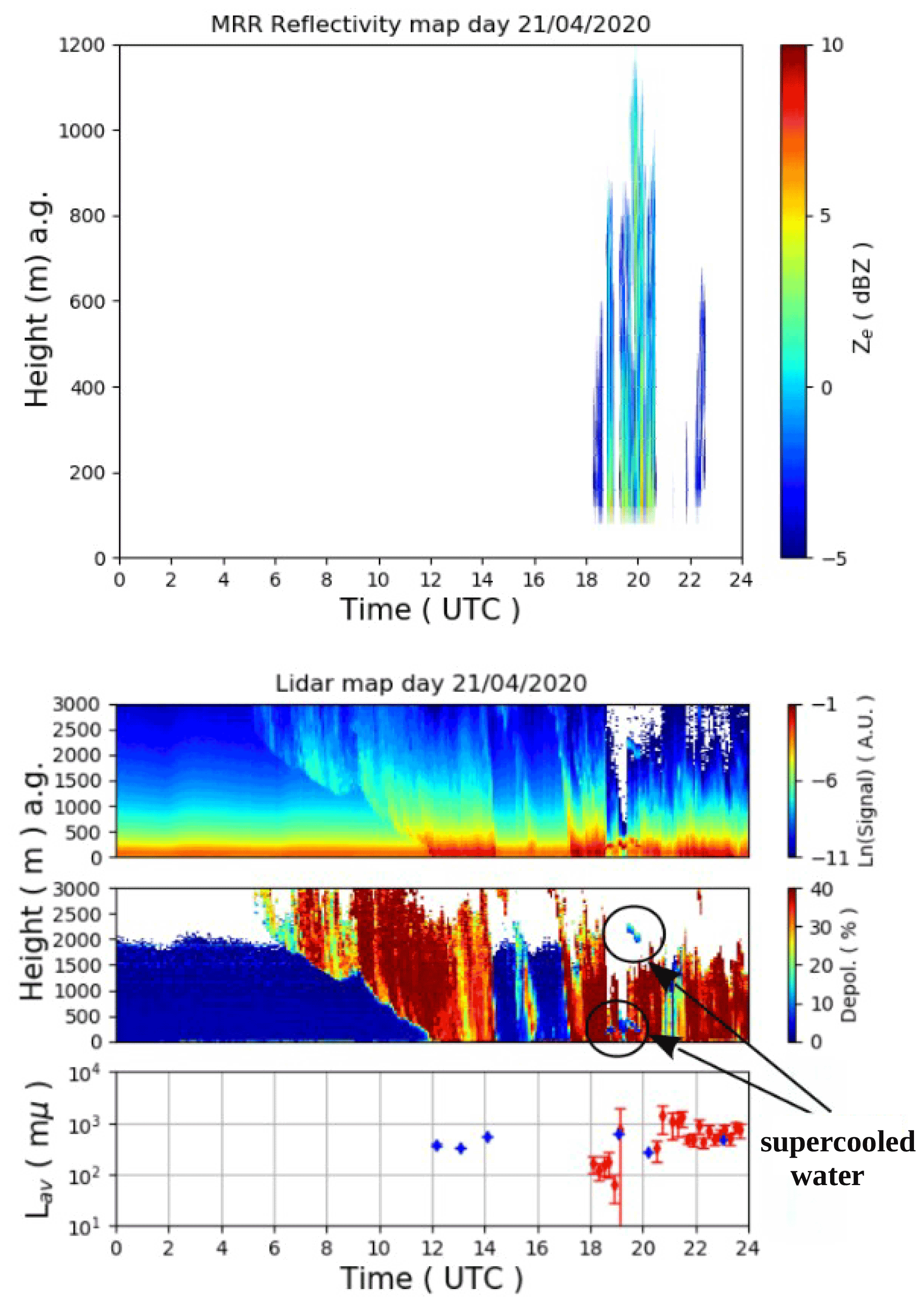
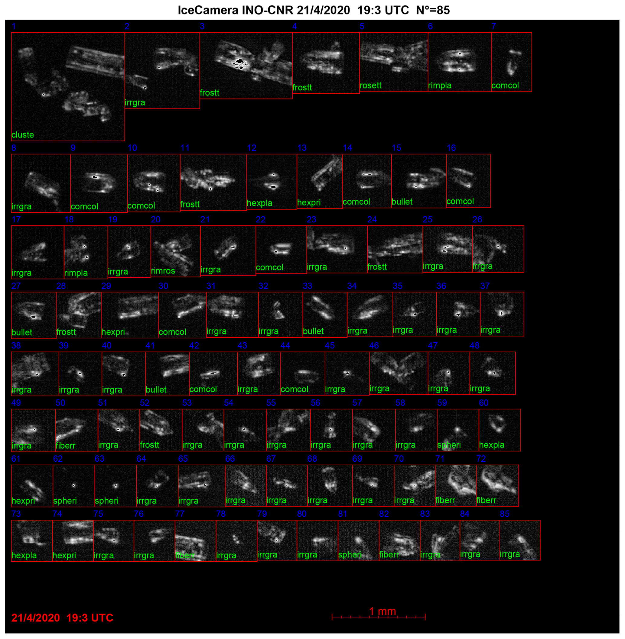
Figure 25 As for Fig. 20, but for the day of 21 April 2020 at 19:03 UTC. At this time, complex aggregates of crystals are also present.

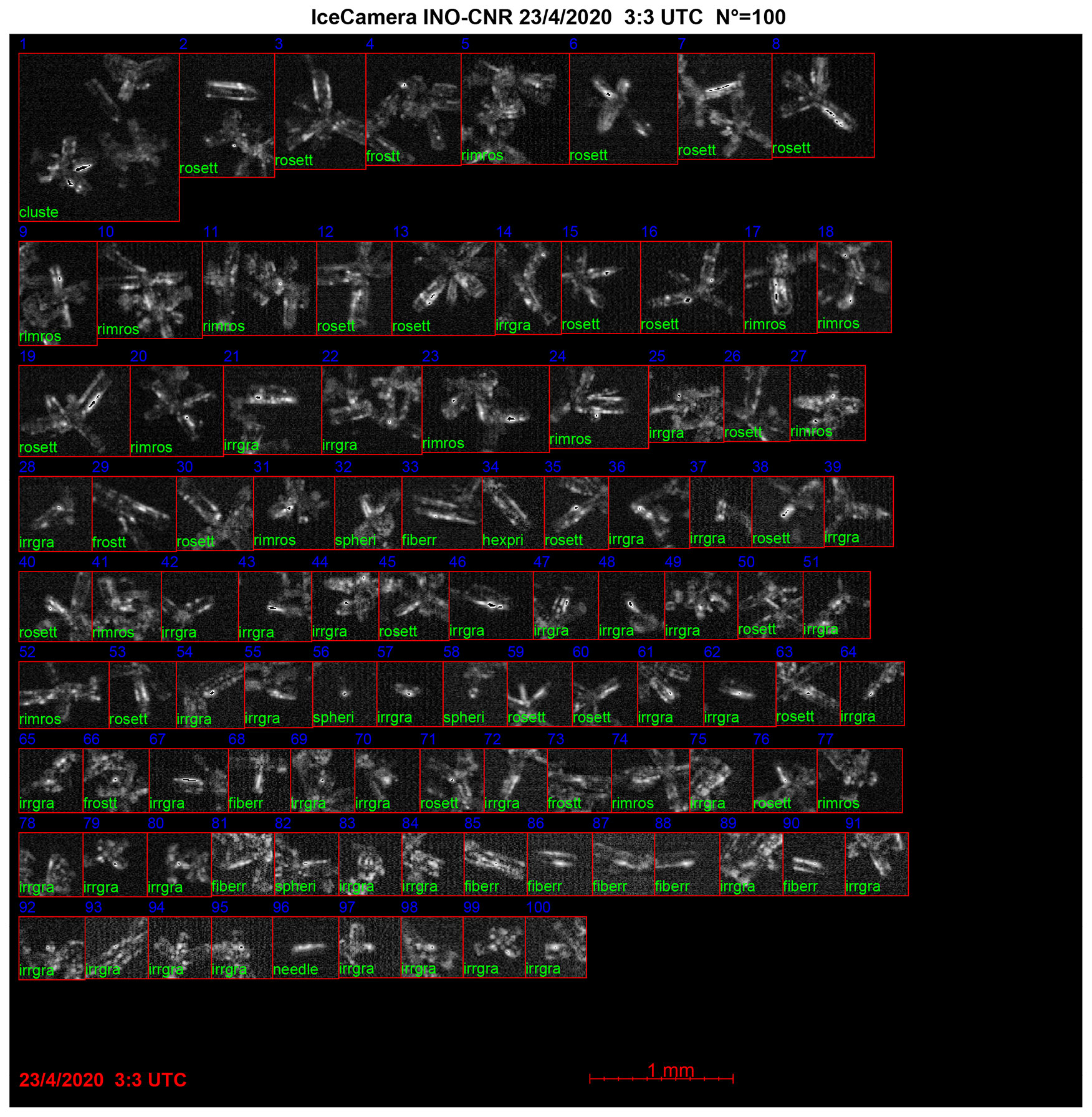
Figure 26 As for Fig. 20, but for the day of 23 April 2020 at 03:03 UTC. At this time, crystals aggregates and bullet rosettes are present.

Some photographs from ICE-CAMERA were available for the comparison, as shown in the lower panels of Figs. 25 and 26. Unfortunately, on 23 April, only a single ice scan measurement was actually provided by the ICE-CAMERA at 03:03 UTC and it did not overlap in time with the radar data. However, the comparison of 21 April shows some agreement with the retrieved L_av. The MRR reflectivity shows high signal values, up to 8 dBz, between 19:00–21:00 UTC on 21 April and between 06:00–11:00 UTC on 23 April. Also during 21 April, a mixed-phase cloud with supercooled water occurred between 19:00 and 20:00 UTC at about 200 m above the ground.

The average retrieved precipitable water vapor (PWV) was found as higher as 2.46 mm for the day of 21 April and 1.33 mm on 23 April, while the average cloud temperatures were about −33 and −38 ^∘C, respectively. The average temperature of the water layer in the REFIR-PAD and MRR measurements was about −23 ^∘C and was located between 200 and 500 m above the ground. In this case, γ was found on average equal to 0.58 and LWP equal to 9.5 g m⁻².

From ICE-CAMERA photograph in Fig. 25, we can see that on day of 21 April at 19:03 UTC, in the middle of the second precipitation event when mixed clouds passed, mostly columnar habits with a minor component of rosettes were present. On 24 April at 03:03 UTC, when the precipitation started and 1.5 h before the MRR signal was detected, the falling ice crystals were mostly rosettes, as shown in the ICE-CAMERA photograph in Fig. 26. Unfortunately, for these days, the HALO-CAMERA images were not available.

5 Conclusions and future perspectives

We presented a new approach to test the consistency of the retrieved ice cloud optical and microphysical properties during precipitating events at Dome C, Antarctica, obtained from two separated portions of the atmospheric spectrum: in the microwave (24 GHz), the observations were provided by the micro rain radar (MRR), while in the far infrared, between 200–980 cm⁻¹, the downwelling spectral radiance measurements were performed with the REFIR-PAD Fourier spectroradiometer.

The MRR was installed at Dome C in 2018 and it has been operating in continuous and unattended mode since then. At the same location, the REFIR-PAD and the tropospheric backscattering lidar have been operating continuously since 2011 and 2008, respectively.

Cloud retrieval properties and the parameters of the particle size distributions were obtained from the synergistic use of the far infrared REFIR-PAD radiance spectra and the backscattering/depolarization lidar profiles.

The average crystal sizes of the precipitating particles were inferred from the photographs taken by the ICE-CAMERA, also installed at Dome C. Furthermore, sky images provided by the HALO-CAMERA were used to detect the solar halos generated by the ice crystals, allowing us to identify and discriminate the hexagonal columns crystal habits responsible for the halos formation.

It is known that the sensitivity of the MRR is limited to the larger falling particles (a priori estimated around 1 mm), due to the large wavelength (12.37 mm) at which the MRR operates. For this reason, we restricted our study to the first 2 years (2019–2020) of the radar measurements when the REFIR-PAD-processed data were already consolidated. We exploited the fact that for large ice particles with effective diameters greater than 80 µm and less than 250 µm, the intercept of the particle size distribution shows a low dependence on the habit type. We modeled the cloud with the aggregate-like crystal habit composed of 10 plates to simulate the radiative transfer and fit the radiance spectra with the Simultaneous Atmospheric and Cloud Retrieval (SACR) code, since for this type of habit the far infrared spectral radiance exhibits higher sensitivity. By analyzing the depolarization of the backscattered lidar signal, we were able to discriminate the presence of only ice or the supercooled water and to determine the top of the precipitating ice cloud through the polar threshold (PT) algorithm.

The retrieval procedure provided the cloud particle effective diameter and optical depth from which we could derive the intercept and the modal radius of the particle size distribution for each observation, which were found to span in wide ranges between 570–2400 µm and 10⁻²–10⁴ cm⁻⁵, respectively, with values in good agreement with the findings of Heymsfield et al. (2013, 2002). These were used to calculate the effective reflectivity at 24 GHz through the scattering databases of Eriksson et al. (2018), which was then compared with MRR observations. The retrieved particle size distribution was also used to assess the mean length of the ice crystals and was compared with those inferred from the ICE-CAMERA images.

We found the best agreement between the reflectivity derived from the REFIR-PAD retrievals and the MRR observations when hexagonal column-like (long columns and thin columns) ice crystals habits and aggregate-like (8-columns and large block aggregate) and $\mathrm{5}/\mathrm{6}$ branches bullet rosettes were used in the calculation of the reflectivity at 24 GHz. These habits show a maximum number of observations with ${\mathit{\chi }}_{\mathrm{red}}^{\mathrm{2}}\simeq \mathrm{1}$ and the correlation coefficient $\mathrm{0.1}\le r^{\mathrm{2}}\le \mathrm{0.3}$. Even though the bullet rosettes ($\mathrm{5}/\mathrm{6}$ branches bullet rosettes) showed low chi square values, the number of observations in accordance with the data was lower with respect to the other habits. The differences arising in the comparison of the reflectivity were mostly due to the difficulty of retrieving the intercept parameter of the size distribution from FIR spectra in the presence of large particles and the low amount of radar data available at the stage of this work. The high occurrence of hexagonal columns and aggregates was confirmed by the ICE-CAMERA photographs. In particular, the presence of hexagonal columns was confirmed by the 22^∘ halos detected by the co-located HALO-CAMERA sky images, as shown in the work by Forster and Mayer (2022) and corroborated by previous measurements at South Pole performed by Lawson et al. (2006). The agreement of both the retrieved parameters of the size distribution confirmed that the retrieval products correctly reproduced the data.

The ICE-CAMERA matrices data were also used to compare the length of the ice crystals with those retrieved by REFIR-PAD, finding a good agreement. These results suggested, based upon the 4 d of data shown here, that the MRR has sensitivity to ice crystals as small as about 600 µm of ice crystal length.

Because of the very low sensitivity of the MRR to the smallest particles, a drastic reduction of the data to be processed was necessary, partially limiting the impact of our study. Because the instruments are all running operationally in an unattended mode, a larger dataset can be assembled that can be used in future studies for confirming the results presented in this work and supporting further considerations with wider statistics.

We are confident that by extending the analysis for at least 5 more years, the results would gain in quality and reliability. With the extended data set, the inference of the effective size of the precipitating crystals in combination with the Doppler velocities provided by the MRR could lead to new analytic relationships between the particle fall velocities and diameters. These relationships could be used to directly estimate the size distribution from the radar power spectra.