the Creative Commons Attribution 4.0 License.
the Creative Commons Attribution 4.0 License.
 | 19 Dec 2022
A new method for calculating average visibility from the relationship between extinction coefficient and visibility
Zefeng Zhang
Hengnan Guo
Hanqing Kang
Jing Wang
Junlin An
Xingna Yu
Jingjing Lv
Bin Zhu
Visibility data are fundamental meteorological observation data widely used in many fields. When using visibility data, it is often necessary to calculate the average visibility, which used to be the arithmetic average of the visibility data directly. In this study, we first analyze the relationship between the visibility, the extinction coefficient, and the atmospheric compositions. Then we propose to use the harmonic average of visibility data as the average visibility, which can better reflect changes in atmospheric extinction coefficients and aerosol concentrations. It is recommended to use the harmonic average visibility in the studies of climate change, atmospheric radiation, air pollution, environmental health, etc.
- Article
(1549 KB) - Full-text XML
- BibTeX
- EndNote


Visibility is a fundamental meteorological parameter (WMO, 1957, 2018) and has a wide range of application scenarios. On the one hand, as an indicator of atmospheric transparency, visibility data are used in many aspects of daily life, such as ground transportation (Ashley et al., 2015; Peng et al., 2017), aviation (Herzegh et al., 2015), and navigation (Debortoli et al., 2019), as well as in scientific research related to weather processes, such as the study of the formation and dissipation of fog. On the other hand, because visibility (v) is determined as a function of the atmospheric extinction coefficient (b) at a given contrast threshold (ε) (Koschmieder, 1924) (Eq. 1), and because the extinction coefficient is predominantly determined by aerosol concentrations (Che et al., 2007), visibility can also be used as a parameter describing atmospheric extinction coefficients (Zhang et al., 2017; Field et al., 2009) and aerosol concentrations (Rosenfeld et al., 2007; Chen et al., 2005), which is widely used in research related to climate change (Rosenfeld et al., 2007; Vautard et al., 2009), atmospheric radiation (Wang et al., 2009; Wu et al., 2014), atmospheric pollution (Gunthe et al., 2021; Yang et al., 2017), and environmental health (Huang et al., 2009; Laden et al., 2006).
A large amount of gridded visibility data have been accumulated through long-term observations at dense measurement sites (Pitchford et al., 2007; Singh et al., 2017). These visibility data are widely used and greatly support much research. Calculating the average visibility is the most frequently performed task when using visibility data (An et al., 2019; Kessner et al., 2013; Zhang et al., 2010). Methodological issues in calculating the average visibility could affect the credibility of the conclusions reached in previous studies using visibility data. Therefore, it is necessary to discuss the method of calculating the average visibility.
There are two variables in Eq. (1), visibility and the extinction coefficient, from which two methods for calculating the average visibility can be derived. The first method directly calculates the arithmetic average of visibility data using Eq. (2), where represents the arithmetic average of visibility data, n is the number of measurements, and vi denotes the visibility obtained in the ith measurement. As can be seen from Eq. (2), the average visibility calculated by the first method is the arithmetic average visibility.
The second method first calculates the arithmetic average of the extinction coefficient, then substitutes the arithmetic average of the extinction coefficient into Eq. (1) to obtain the average visibility; the specific derivation process and results are shown in Eq. (3). Specifically, first substitute the visibility measurement vi into Eq. (1) to obtain the corresponding extinction coefficient bi in the ith measurement. Then, calculate the arithmetic average of a total of n extinction coefficients, denoted as . Finally, substitute the arithmetic average of the extinction coefficient into Eq. (1) to obtain the average visibility . As can be seen from Eq. (3), the average visibility calculated by the second method is the harmonic average visibility.
Equation (2) gives the arithmetic average visibility, and Eq. (3) gives the harmonic average visibility. It is clear that the values of average visibility calculated by the two methods are different. This is because atmospheric visibility is constantly changing, and it has been mathematically proven that, unless all values used to calculate the average are the same, the arithmetic average is always greater than the harmonic average (Ferger, 1931).
The question arises as to whether the average visibility used in practical work should be the arithmetic average visibility calculated by Eq. (2) or the harmonic average visibility calculated by Eq. (3). To date, arithmetic average visibility has been used in studies (An et al., 2019; Kessner et al., 2013; Rosenfeld et al., 2007; Singh et al., 2017; Zhang et al., 2017), and harmonic average visibility has never been an option so that when studies refer to average visibility, it is calculated directly using Eq. (2) without the need for clarification. However, no theoretical justification has been given in past studies for using the arithmetic average visibility rather than the harmonic average visibility. It is true that the arithmetic average visibility is more intuitive; this does not exclude the possibility that the option of the harmonic average visibility has been overlooked in the past. Therefore, a more in-depth discussion is necessary.
The first thing to do is to compare the difference in numerical values of the average visibility obtained by the two methods. If the difference is negligible, there is no point in discussing this issue, and the arithmetic average visibility obtained from Eq. (2) can be used with small error. However, if the difference is considerable, it is necessary to analyze the difference in physical meaning between arithmetic average visibility and harmonic average visibility and then select the appropriate calculation method for average visibility in different scenarios according to the purpose of using visibility data.
To visualize the magnitude of the numerical difference between arithmetic average visibility and harmonic average visibility, we analyzed the visibility data measured at 1 min resolution by a CJY-1 visibility meter (CAMA Measurement & Control Equipments Co. Ltd.) on the campus of the Nanjing University of Information Science & Technology in Nanjing, China, during 2010–2017. The details regarding the observation site and instruments are given in Zhang et al. (2017).
The hourly, daily, monthly, and yearly arithmetic average visibility and harmonic average visibility are shown in Fig. 1a and b, respectively. By substituting the values of average visibility during the corresponding period shown in Fig. 1a and b into Eq. (4), we obtain the relative deviation of the hourly, daily, monthly, and yearly arithmetic average visibility from harmonic average visibility. Figure 1c shows the distribution of the magnitude of relative deviation. The value of 96.3 in the lower-left corner of Fig. 1c indicates that 96.3 % of the relative deviation of the hourly average visibility falls within the range of 0 %–10 %.
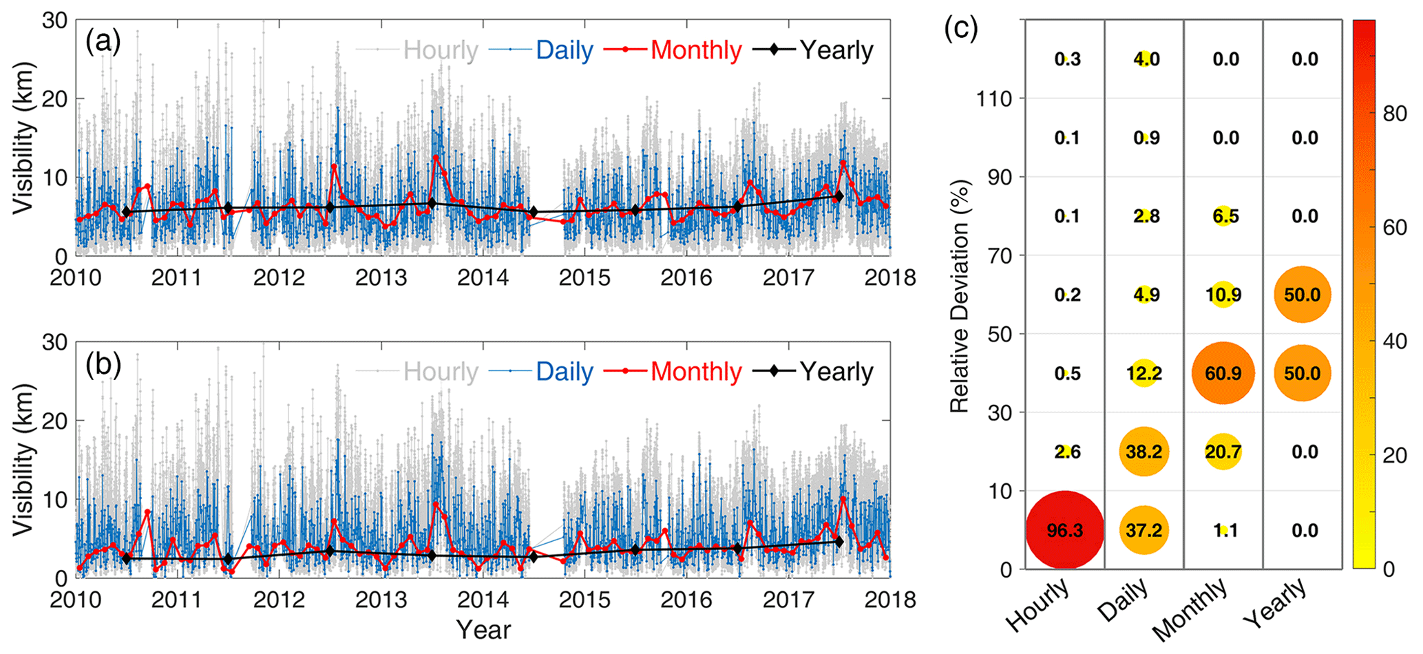
Figure 1Comparison of arithmetic average visibility and harmonic average visibility: (a) arithmetic average visibility calculated using Eq. (2). (b) Harmonic average visibility calculated using Eq. (3). (c) Distribution of the relative deviation of arithmetic average visibility from harmonic average visibility.
As shown in Fig. 1, the arithmetic average visibility calculated using Eq. (2) (Fig. 1a) is always greater than the harmonic average visibility calculated using Eq. (3) (Fig. 1b); therefore, all values of the relative deviation lie in the range of greater than zero. The results in Fig. 1 are not a coincidence because of the specificity of the measurement data, but an inevitable result that will appear when calculating the average of any visibility measurement data using Eqs. (2) and (3). It has been mathematically proven that, unless all values used to calculate the average are the same, the arithmetic average is always greater than the harmonic average; the greater the variation in the data, the greater the difference between the two.
The relationship between the arithmetic average and the harmonic average can explain the distribution of relative deviation values in Fig. 1c. The range of the measured visibility values is typically related to the observation period. The longer the duration of the observation, the larger the range of the measured visibility data. Therefore, the longer the observation period chosen to calculate the average visibility, the larger the relative deviation of the arithmetic average visibility from the harmonic average visibility. It is not difficult to understand why the relative deviation of the yearly average is larger than that of the monthly average, which is larger than that of the hourly average, according to the distribution of the relative deviation shown in Fig. 1c.
Regarding the relative deviation of yearly and monthly arithmetic average visibility from harmonic average visibility (Fig. 1c), most of the values fall within the range of 30 % to 70 %, which is far greater than the typical range of measurement error of visibility meters (WMO, 2018). Regarding the relative deviation of hourly and daily average visibility, although most of the values are less than 30 %, this does not mean that the difference between the arithmetic average and the harmonic average can be ignored. Because atmospheric visibility can sometimes change significantly in a short time, a topic of particular interest in previous studies, at which time the average visibility calculated by the two methods can be quite different.
In summary, as long as the atmospheric visibility is variable, the values of arithmetic average visibility and harmonic average visibility will not be the same, and the magnitude of the difference between them is related to the intensity of the change in visibility. Therefore, the difference between the two calculation methods cannot be ignored in large-scale and long-term studies. Even for small-scale and short-term studies, the difference is not negligible when there is a significant change in visibility.
3.1 Discussion of the extinction coefficient and visibility
To understand the difference in physical meaning between arithmetic average visibility and harmonic average visibility, it is necessary to understand the characteristics of the two physical quantities, extinction coefficient and visibility. To this end, we design a thought experiment.
Assume there is a system where there is a total of n components affecting the extinction coefficient. The mass concentration of the ith component is mi, and the mass extinction coefficient is Mi. We carry out a thought experiment, and the experimental procedures and corresponding results are recorded in Table 1.
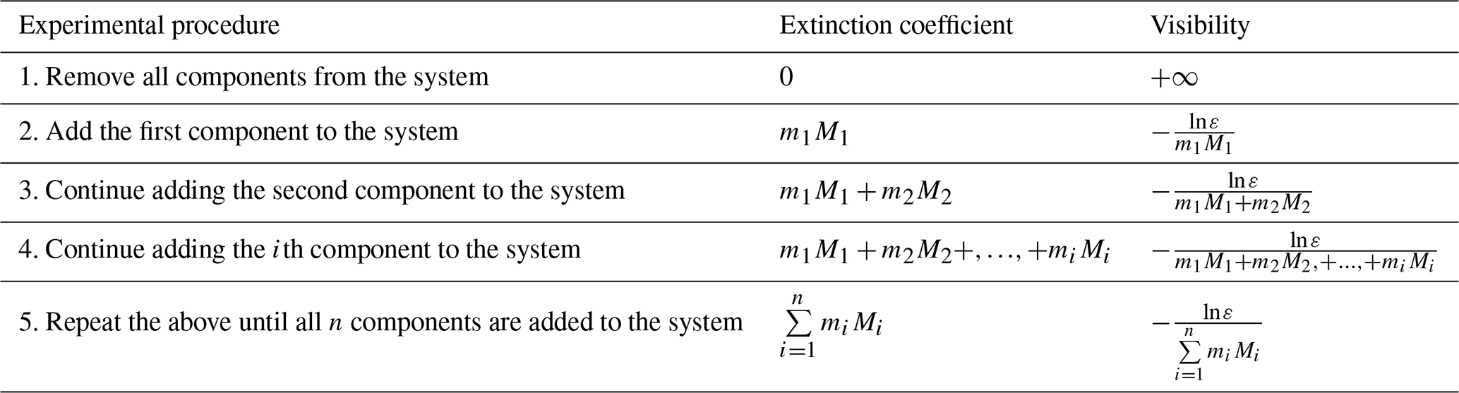
Two conclusions can be drawn from the results of the thought experiment recorded in Table 1. It should be noted that these two conclusions are not new knowledge but the basis for subsequent discussion.
The first conclusion is that the concentration and the optical properties of the components determine the extinction coefficient and the visibility of the system. This suggests that the changes in the extinction coefficient and visibility of the system should logically match the changes in the mass concentration and mass extinction coefficient of the components in the system.
The second conclusion is that the extinction coefficient is an extensive quantity, whereas the visibility is neither an extensive nor an intensive quantity. This is because the extinction coefficient is proportional to the amount of matter in the system, suggesting that the extinction coefficient is an extensive quantity. The visibility decreases as the amount of matter in the system increases, suggesting that visibility is not an extensive quantity. The magnitude of visibility varies with the concentration of the components in the system, so it is not a characteristic property or an intensive quantity of the components. Therefore, the summation of visibility data is just a useful statistic without real physical meaning.
3.2 Physical meaning of arithmetic average visibility and harmonic average visibility
Simulated measurements are generated in order to discuss the physical meaning of arithmetic average visibility and harmonic average visibility. Assuming that a total of n measurements are made with the same instrument, at the same site, at the same time interval, and the measurement results are considered reliable, Eq. (5) relates the mass concentration (mj) and the mass extinction coefficient (Mj) of the sample to the extinction coefficient, and to the visibility in the jth observation.
Then we calculate the average extinction coefficient and average visibility with three methods, respectively.
Method 1. Based on the first conclusion in Sect. 3.1, the average extinction coefficient and average visibility were calculated using the concentrations and optical properties of the samples during the observation period, as the definition implies. First, calculate the average mass concentration and the average mass extinction coefficient during the observation period, as shown in Eq. (6). Then, calculate the average extinction coefficient and average visibility using the average mass concentration and the average mass extinction coefficient during the observation period, as shown in Eq. (7).
Method 2. Substitute the observed mass concentration and mass extinction coefficient with Eq. (2) to obtain the arithmetic average visibility, which is then substituted with Eq. (1) to obtain the corresponding average extinction coefficient, as shown in Eq. (8).
Method 3. Substitute the observed mass concentration and mass extinction coefficient with Eq. (3) to obtain the harmonic average visibility, which is then substituted with Eq. (1) to obtain the corresponding average extinction coefficient, as shown in Eq. (9).
The average visibility and average extinction coefficient calculated by the three methods are now compared and analyzed. A comparison of Eqs. (7) and (9) indicates that the expression of the average visibility and the expression of the average extinction coefficient are identical respectively, while the expressions in Eq. (8) are different from those in Eqs. (7) and (9).
The reason for this can be explained by the second conclusion given in Sect. 3.1. All three methods perform summation. Methods 1 and 3 both carry out the summation over extensive quantities, i.e., the mass and the extinction coefficient, so that their corresponding physical meanings are clear. Methods 1 and 3 actually describe the same physical process, i.e., the mixing process. However, Method 2 carries out the summation over the visibility, which is neither an extensive quantity nor an intensive quantity, so that the results of the summation of visibility are just numerical values with no corresponding physical meaning. Therefore, the arithmetic average visibility has no real physical meaning.
The difference in the physical meaning of arithmetic average visibility and harmonic average visibility leads to the difference in the derived expressions of the average extinction coefficient. It can be seen from Eqs. (7) and (9) that the expression of the average extinction coefficient derived from the harmonic average visibility (Eq. 9) is identical to that derived from the definition of the extinction coefficient (Eq. 7). However, a comparison of Eqs. (7) and (8) indicates that the expression of the average extinction coefficient derived from the arithmetic average visibility (Eq. 8) differs from that derived from the definition of the extinction coefficient (Eq. 7). This suggests that we should use the harmonic average visibility rather than the arithmetic average visibility when using average visibility data to obtain average extinction coefficient. Considering that the main contribution to atmospheric extinction comes from aerosol particles, it is also appropriate to use harmonic average visibility data for research on aerosols using visibility data.
In summary, if the purpose is to numerically describe the measured visibility data, then the calculation of average visibility can be treated as a statistical problem, and the arithmetic average visibility can be used to represent the average visibility. However, if the average visibility is used as a parameter to characterize changes in atmospheric extinction coefficients and aerosol concentrations, especially in research related to climate change, atmospheric radiation, atmospheric pollution, environmental health, etc., then the calculation of average visibility should be treated as a physical problem, and the harmonic average visibility should be used to represent the average visibility.
This study proposes a new method for calculating the average of visibility data, i.e., harmonic average visibility. The main differences between the proposed harmonic average visibility from the previously used arithmetic average visibility are as follows:
-
The numerical values of harmonic average visibility and arithmetic average visibility are different. The values of harmonic average visibility are always smaller than the corresponding arithmetic average visibility, and the difference between them becomes larger as the observed visibility values fluctuate more strongly. Therefore, the method for calculating the average visibility should be carefully selected when analyzing large-scale or long-term visibility data and when analyzing local visibility data with large changes within a short period of time.
-
Compared to the arithmetic average visibility, the harmonic average visibility can better represent changes in average atmospheric extinction coefficients and average aerosol concentrations. Therefore, we recommend preferentially using harmonic average visibility when calculating the average of visibility data in research related to climate change, atmospheric radiation, atmospheric pollution, environmental health, etc.
The data supporting the conclusions have been deposited in Zenodo (https://doi.org/10.5281/zenodo.5025882; Zhang, 2021).
ZZ conceived and designed the experiments, contributed to the analysis of the results, and wrote the paper. HG generated the figures. HK, JW, JA, XY, JL, and BZ were involved in the discussions and helped in the data analysis.
The contact author has declared that none of the authors has any competing interests.
Publisher’s note: Copernicus Publications remains neutral with regard to jurisdictional claims in published maps and institutional affiliations.
This work was supported by the National Key Research and Development Program of China (no. 2019YFC0214604). We thank WeiWei Wang, Li Xia, and Jiade Yan for offering visibility data and maintaining the observation site used in this study.
This research has been supported by the National Key Research and Development Program of China, Chinese Polar Environment Comprehensive Investigation and Assessment Programs (grant no. 2019YFC0214604).
This paper was edited by Francis Pope and reviewed by three anonymous referees.
An, Z., Huang, R.-J., Zhang, R., Tie, X., Li, G., Cao, J., Zhou, W., Shi, Z., Han, Y., Gu, Z., and Ji, Y.: Severe haze in northern China: A synergy of anthropogenic emissions and atmospheric processes, P. Natl. Acad. Sci. USA, 116, 8657–8666, https://doi.org/10.1073/pnas.1900125116, 2019.
Ashley, W. S., Strader, S., Dziubla, D. C., and Haberlie, A.: Driving blind: Weather-related vision hazards and fatal motor vehicle crashes, B. Am. Meteorol. Soc., 96, 755–778, https://doi.org/10.1175/bams-d-14-00026.1, 2015.
Che, H., Zhang, X., Li, Y., Zhou, Z., and Qu, J. J.: Horizontal visibility trends in China 1981–2005, Geophys. Res. Lett., 34, L24706, https://doi.org/10.1029/2007gl031450, 2007.
Chen, L. H., Knutsen, S. F., Shavlik, D., Beeson, W. L., Petersen, F., Ghamsary, M., and Abbey, D.: The Association between Fatal Coronary Heart Disease and Ambient Particulate Air Pollution: Are Females at Greater Risk?, Environ. Health Persp., 113, 1723–1729, https://doi.org/10.1289/ehp.8190, 2005.
Debortoli, N. S., Clark, D. G., Ford, J. D., Sayles, J. S., and Diaconescu, E. P.: An integrative climate change vulnerability index for Arctic aviation and marine transportation, Nat. Commun., 10, 2596, https://doi.org/10.1038/s41467-019-10347-1, 2019.
Field, R. D., van der Werf, G. R., and Shen, S. S. P.: Human amplification of drought-induced biomass burning in Indonesia since 1960, Nat. Geosci., 2, 185–188, https://doi.org/10.1038/ngeo443, 2009.
Gunthe, S. S., Liu, P., Panda, U., Raj, S. S., Sharma, A., Darbyshire, E., Reyes-Villegas, E., Allan, J., Chen, Y., Wang, X., Song, S., Pöhlker, M. L., Shi, L., Wang, Y., Kommula, S. M., Liu, T., Ravikrishna, R., McFiggans, G., Mickley, L. J., Martin, S. T., Pöschl, U., Andreae, M. O., and Coe, H.: Enhanced aerosol particle growth sustained by high continental chlorine emission in India, Nat. Geosci., 14, 77–84, https://doi.org/10.1038/s41561-020-00677-x, 2021.
Ferger, W. F.: The Nature and Use of the Harmonic Mean, J. Am. Stat. Assoc., 26, 36–40, https://doi.org/10.1080/01621459.1931.10503148, 1931.
Herzegh, P., Wiener, G., Bateman, R., Cowie, J., and Black, J.: Data fusion enables better recognition of ceiling and visibility hazards in aviation, B. Am. Meteorol. Soc., 96, 526–532, https://doi.org/10.1175/bams-d-13-00111.1, 2015.
Huang, W., Tan, J., Kan, H., Zhao, N., Song, W., Song, G., Chen, G., Jiang, L., Jiang, C., Chen, R., and Chen, B.: Visibility, air quality and daily mortality in Shanghai, China, Sci. Total Environ., 407, 3295–3300, https://doi.org/10.1016/j.scitotenv.2009.02.019, 2009.
Kessner, A. L., Wang, J., Levy, R. C., and Colarco, P. R.: Remote sensing of surface visibility from space: A look at the United States East Coast, Atmos. Environ., 81, 136–147, https://doi.org/10.1016/j.atmosenv.2013.08.050, 2013.
Koschmieder, H.: Theorie der horizontalen sichtweite, Beiträge zur Physik der freien Atmosphäre, Meteorol. Z., 12, 33–55, 1924.
Laden, F., Schwartz, J., Speizer, F. E., and Dockery, D. W.: Reduction in fine particulate air pollution and mortality, Am. J. Resp. Crit. Care, 173, 667–672, https://doi.org/10.1164/rccm.200503-443OC, 2006.
Peng, Y., Abdel-Aty, M., Shi, Q., and Yu, R.: Assessing the impact of reduced visibility on traffic crash risk using microscopic data and surrogate safety measures, Transport. Res. C-Emer., 74, 295–305, https://doi.org/10.1016/j.trc.2016.11.022, 2017.
Pitchford, M., Malm, W., Schichtel, B., Kumar, N., Lowenthal, D., and Hand, J.: Revised algorithm for estimating light extinction from IMPROVE particle speciation data, J. Air Waste Manag. Assoc., 57, 1326–1336, https://doi.org/10.3155/1047-3289.57.11.1326, 2007.
Rosenfeld, D., Dai, J., Yu, X., Yao, Z., Xu, X., Yang, X., and Du, C.: Inverse relations between amounts of air pollution and orographic precipitation, Science, 315, 1396–1398, https://doi.org/10.1126/science.1137949, 2007.
Singh, A., Bloss, W. J., and Pope, F. D.: 60 years of UK visibility measurements: impact of meteorology and atmospheric pollutants on visibility, Atmos. Chem. Phys., 17, 2085–2101, https://doi.org/10.5194/acp-17-2085-2017, 2017.
Vautard, R., Yiou, P., and van Oldenborgh, G. J.: Decline of fog, mist and haze in Europe over the past 30 years, Nat. Geosci., 2, 115–119, https://doi.org/10.1038/ngeo414, 2009.
Wang, K., Dickinson, R. E., and Liang, S.: Clear sky visibility has decreased over land globally from 1973 to 2007, Science, 323, 1468–1470, 2009.
WMO: Ninth Session of the Executive Committee: Abridged Report with Resolutions, World Meteorological Organization, Geneva, Switzerland, WMO-No. 67, 335 pp., 1957.
WMO: Guide to instruments and methods of observation, Volume I – Measurement of Meteorological Variables, World Meteorological Organization, Geneva, Switzerland, WMO-No. 8, 581 pp., ISBN 978-92-63-10008-5, https://library.wmo.int/doc_num.php?explnum_id=11386 (last access: 15 December 2022), 2018.
Wu, J., Luo, J., Zhang, L., Xia, L., Zhao, D., and Tang, J.: Improvement of aerosol optical depth retrieval using visibility data in China during the past 50 years, J. Geophys. Res.-Atmos., 119, 13370–13387, https://doi.org/10.1002/2014jd021550, 2014.
Yang, Y., Russell, L. M., Lou, S., Liao, H., Guo, J., Liu, Y., Singh, B., and Ghan, S. J.: Dust-wind interactions can intensify aerosol pollution over eastern China, Nat. Commun., 8, 15333, https://doi.org/10.1038/ncomms15333, 2017.
Zhang, Q. H., Zhang, J. P., and Xue, H. W.: The challenge of improving visibility in Beijing, Atmos. Chem. Phys., 10, 7821–7827, https://doi.org/10.5194/acp-10-7821-2010, 2010.
Zhang, Z.: Average Visibility Data, Version 1, Zenodo [data set], https://doi.org/10.5281/zenodo.5025882, 2021.
Zhang, Z., Shen, Y., Li, Y., Zhu, B., and Yu, X.: Analysis of extinction properties as a function of relative humidity using a κ-EC-Mie model in Nanjing, Atmos. Chem. Phys., 17, 4147–4157, https://doi.org/10.5194/acp-17-4147-2017, 2017.
- Abstract
- Introduction
- The numerical difference between arithmetic average visibility and harmonic average visibility
- Physical meaning of the two calculation methods of average visibility
- Conclusions
- Data availability
- Author contributions
- Competing interests
- Disclaimer
- Acknowledgements
- Financial support
- Review statement
- References