Doppler spectra from DWD's operational C-band radar birdbath scan: sampling strategy, spectral postprocessing, and multimodal analysis for the retrieval of precipitation processes

This study explores the potential of using Doppler (power) spectra from vertically pointing C-band radar birdbath scans to investigate precipitating clouds above the radar. First, the new birdbath scan strategy for the network of dual-polarization C-band radars operated by the German Meteorological Service (Deutscher Wetterdienst, DWD) is outlined, and a novel spectral postprocessing and analysis method is presented. The postprocessing algorithm isolates the weather signal from non-meteorological contributions in the radar output based on polarimetric attributes, identifies the statistically significant precipitation modes contained in each Doppler spectrum, and calculates characteristics of every precipitation mode as well as multimodal properties that describe the relation among different modes when more than a single mode is identified. To achieve a high degree of automation and flexibility, the postprocessing chain combines classical signal processing with clustering algorithms. Uncertainties in the calculated modal and multimodal properties are estimated from the small variations associated with smoothing the measured radar signal.

The analysis of five birdbath scans recorded at different radar sites and for various precipitation conditions delivers reliable profiles of the derived modal and multimodal properties for two snowfall cases and for stratiform precipitation above and below the melting layer. To help identify the dominant precipitation growth mechanism, Doppler spectra from DWD's birdbath scans can be used to retrieve the typical degree of riming for individual snow modes. Here, the automatically identified snow modes span a wide range of riming conditions with estimated rime mass fractions (RMFs) of up to RMF>0.5. The evaluation of Doppler spectra inside the melting layer and for an intense frontal shower, with observed radar reflectivities of up to about 40 dBZ, occasionally shows erroneously identified precipitation modes and spurious results for the calculated higher-order Doppler moments of skewness and kurtosis. Nonetheless, the Doppler spectra from DWD's operational C-band radar birdbath scan provide a detailed view into the precipitating clouds and allow for calculating a high-resolution profile of radar reflectivity, mean Doppler velocity, and spectral width even in intense frontal precipitation.

1 Introduction

Polarimetric radar measurements of precipitating clouds provide crucial information both for fundamental research into precipitation processes and for operational weather services (Ryzhkov and Zrnic, 2019). For example, assigning general classes of precipitation particles, such as rain, light rain, dry snow, wet snow, graupel, and hail, to polarimetric radar data based on radar scattering calculations allows for identifying the dominant (in terms of the radar signature) precipitation particle type in each radar bin, called a hydrometeor classification (e.g., Marzano et al., 2007, 2008; Park et al., 2009; Dolan and Rutledge, 2009; Dolan et al., 2013; Al-Sakka et al., 2013; Bechini and Chandrasekar, 2014; Thompson et al., 2014; Frech and Steinert, 2015; Grazioli et al., 2015; Besic et al., 2016; Steinert et al., 2021). Furthermore, rain and snowfall rate or water content can be estimated from different combinations of measured polarimetric variables to improve quantitative precipitation estimates that were previously based only on measured radar reflectivity (e.g., Vivekanandan et al., 2004; Marzano et al., 2010; Bukovcic et al., 2018). Quantitative parameters specifying typical ice particle shape and orientation can also be retrieved from polarimetric radar measurements (e.g., Melnikov and Straka, 2013; Melnikov, 2017; Myagkov et al., 2016). On a more fundamental level, characteristic features, or fingerprints, of precipitation processes observed with polarimetric radars have advanced the discussion of which microphysical processes drive the formation and evolution of precipitating clouds (e.g., Kumjian et al., 2014; Kumjian and Lombardo, 2017; Moisseev et al., 2015; Ryzhkov et al., 2016; Kaltenboeck and Ryzhkov, 2016; Griffin et al., 2018). Physical conclusions or quantitative retrieval results from such polarimetric radar observations can then also be used to challenge and help improve the representation of precipitation processes in atmospheric models for weather forecasting and climate research (e.g., Trömel et al., 2021).

To exploit the wealth of information offered by polarimetric radar measurements, many national weather services operate networks of dual-polarization weather radars at C- or S-band frequencies. The German Meteorological Service (Deutscher Wetterdienst, DWD), for example, manages a network of 17 C-band radars that continuously scan the atmosphere at low elevation angles. These C-band weather radars cover a large area within a short update cycle and can resolve a broad range of precipitation intensities up to hailstorms (Bringi and Chandrasekar, 2001; Ryzhkov and Zrnic, 2019). Higher-frequency cloud radars, operating at Ka- or W-band, for example, instead allow for a more granular view of precipitating and non-precipitating clouds. As such cloud radars are much more affected by atmospheric attenuation than longer-wavelength weather radars, they are used to probe a much smaller part of the atmosphere closer to the radar, and they are often set up as vertically pointing atmospheric profilers. While being limited to moderate precipitation intensities, vertically pointing Doppler cloud radars can additionally provide high-resolution profiles of Doppler spectra (e.g., Kollias et al., 2007). Here, the overall signal power remitted from the cloud and precipitation particles within each atmospheric radar resolution volume is further subdivided into the individual contributions from a wide spectrum of Doppler velocities that indicate the relative movement of the precipitation particles along the line of sight of the radar.

Based on the dependence of the terminal fall velocity of a hydrometeor on its mass, phase, and shape, Doppler spectra offer a detailed view into clouds that pass over the radar. Therefore, several studies have leveraged vertically pointing Doppler cloud radar measurements to detect supercooled liquid water in mixed-phase clouds (Shupe et al., 2004; Luke et al., 2010) or to analyze riming events (Kalesse et al., 2016). These phenomena are difficult to identify from polarimetric radar observations alone (Moisseev et al., 2017; Li et al., 2018; Vogel and Fabry, 2018), unless riming is sufficiently strong to cause a characteristic “sagging” of the melting-layer bright band toward lower altitudes (Kumjian et al., 2016). A detailed analysis of such Doppler spectra requires careful postprocessing to identify and separate the spectral signatures of different hydrometeor populations that may occur simultaneously within the same radar resolution volume, e.g., slower-falling, small supercooled liquid drops and faster-falling rimed snow particles (following the methodology proposed by Williams et al., 2018, for example). By interpreting the mean velocity of the Doppler spectra as the typical precipitation particle fall velocity, the degree of riming can also be estimated from vertically pointing Doppler radar observations (Kneifel and Moisseev, 2020). When higher-order moments of the recorded Doppler spectra are calculated, they provide additional valuable information for retrieving microphysical cloud properties (Maahn and Löhnert, 2017).

While these studies have extracted great value from Doppler spectra recorded by vertically pointing cloud radars, vertically pointing measurements from longer-wavelength C- or S-band radars are rarely explored for studying precipitation processes (e.g., by Moisseev et al., 2015). Some C- and S-band radar designs do not allow vertically pointing measurements; and where such observations are available, they are mostly used for quality control of polarimetric radar data. For DWD's C-band radars, for example, a birdbath scan (where the radar antenna rotates a full 360^∘ while pointing vertically upward, i.e., at a constant elevation angle of 90^∘) has been used routinely to monitor the calibration of the differential reflectivity (Frech and Hubbert, 2020), one of the polarimetric variables required as input for the Hymec hydrometeor classification scheme at the DWD (Steinert et al., 2021).

To investigate how vertically pointing C-band radar observations can be used for the analysis of precipitation processes, this study quantitatively interprets Doppler spectra collected by the new DWD birdbath scan that was introduced into the operational scanning cycle of the German C-band radar network in the spring of 2021. Section 2 gives an overview of the sampling strategy and describes a postprocessing method for calculating key properties of the Doppler spectra and estimating the corresponding uncertainties. Here, a flexible spectral postprocessing method is proposed that first separates the weather signal from non-meteorological contributions based on polarimetric attributes and then identifies all statistically significant peaks in the Doppler spectra to reveal multiple simultaneously occurring precipitation regimes. Both tasks are accomplished by leaning on existing clustering algorithms, thereby illustrating how data mining techniques can enhance classical signal processing methods. Analysis results for different precipitation conditions and at different radar sites are discussed in Sect. 3. While the overall focus of this study is on frozen precipitation, the results also provide insights into the formation and evolution of rain. Finally, the capabilities and limitations of the presented methods are summarized in Sect. 4.

2 Methods

The operational DWD birdbath scan that is presented in Sect. 2.1 aims at providing Doppler (power) spectra at high spatial and spectral resolutions. To fully take advantage of these detailed spectral data, a novel multistep postprocessing method is proposed in Sect. 2.2–2.4, focusing on objectively identifying and quantifying the precipitation modes contained in every Doppler spectrum.

2.1 DWD birdbath scan

The German Meteorological Service (Deutscher Wetterdienst, DWD) operates a network of 17 dual-polarization C-band Doppler radars to monitor the lower atmosphere above Germany. An additional research radar that is quasi-identical to the operational DWD radar systems is located at the Meteorological Observatory Hohenpeissenberg (MOHp) in pre-alpine southern Germany (MOHp radar latitude (lat): 47.80151^∘ N, longitude (long): 11.00929^∘ E; altitude (alt): 1006 m above sea level (a.s.l.)). The DWD research radar is used to test hardware and software upgrades or new scan strategies and analysis methods before they are implemented across the national C-band radar network. If a nearby operational radar fails, the research radar can also be included in the operational service. Detailed descriptions of DWD radar systems and data processing are given in prior studies (Frech et al., 2013, 2017, 2019).

The DWD operational radar scanning cycle is composed of multiple individual scans that aim at capturing essential meteorological characteristics for weather forecasting or allow for monitoring the quality and consistency of the radar measurements (Frech and Steinert, 2015). The entire scanning cycle is repeated every 5 min. In this study, we focus only on one component of the scanning cycle: the vertically pointing birdbath scan. The birdbath scan was originally introduced together with the network upgrade from non-polarimetric to dual-polarization radars in 2009, and the primary application up to now has been the calibration of the differential reflectivity (Frech and Hubbert, 2020). In the spring of 2021, the DWD birdbath scan strategy was modified to record C-band Doppler spectra. Since then, the Doppler spectra have been saved routinely and are thus available for studying precipitating clouds at all DWD C-band radar sites in detail. Important parameters of the updated birdbath scan strategy and of the resulting Doppler spectra are listed in Table 1.

Table 1 Characteristics of the DWD operational birdbath scan and Doppler spectra.

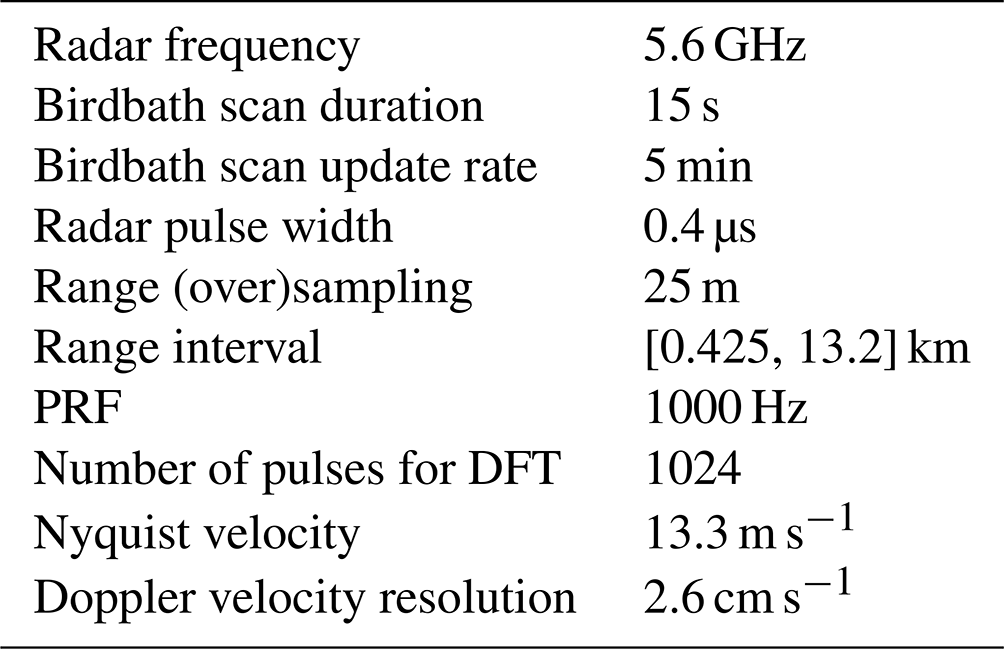
PRF: pulse repetition frequency; DFT: discrete Fourier transform.

Rotating the antenna at an intermediate speed of 24^∘ s⁻¹ and using the finest range sampling available, each birdbath scan essentially provides a 15 s snapshot of the atmospheric column above the radar between heights of 0.425 and 13.2 km in steps of 25 m. Here, range oversampling at 25 m offers more spatial structure in DWD's radar birdbath data than the intrinsic resolution of 60 m. With a pulse repetition frequency (PRF) of 1000 Hz, an unambiguous Doppler velocity range of $-\mathrm{13.3}\le v\le \mathrm{13.3}$ m s⁻¹ is achieved. In this study, negative Doppler velocities indicate particles moving toward the radar and thus falling downward.

For the two orthogonal polarization channels $p=H,V$, the Doppler spectra ${\widehat{S}}_p\left(f\right)$ with Doppler frequency f are estimated at each height from the discrete Fourier transform (DFT, F_p(f)) of the received I(n-phase) and Q(uadrature) samples s_p, where the DFTs are calculated for K=1024 consecutive radar pulses:

$$\begin{array}{}\text{(1)}& {\displaystyle }{F}_p\left(f\right)=\sum _{k=\mathrm{0}}^{K-\mathrm{1}}{d}_k{s}_{p;k}\exp (-i\mathrm{2}\mathit{\pi }kf),\text{(2)}& {\displaystyle }{\widehat{S}}_p\left(f\right)=\mathrm{10}{\log }_{\mathrm{10}}\left[F_p\left(f\right)F_p^{\ast }\left(f\right)\right].\end{array}$$

In Eq. (1), the tapering function d_k is given by the 3-term Blackman–Harris window that achieves the minimum sidelobe level of −67 dB (Harris, 1978, Fig. 24). The Doppler spectra ${\widehat{S}}_p\left(f\right)$ in Eq. (2) then decompose the total received power into 1024 spectral contributions at a resolution of $\mathrm{\Delta }f\equiv \mathrm{\Delta }v=\mathrm{2.6}$ cm s⁻¹, and the power in each spectral bin is expressed as an uncalibrated dB value that is proportional to the power spectral density commonly employed in electrical engineering (Yu et al., 2012). These radar settings ultimately produce 15 separate Doppler spectra in the H and V polarization channels at each height.

The radar settings were chosen to obtain a wide unambiguous velocity range, which requires a high PRF, and a fine Doppler velocity resolution, which requires a high number of radar pulses for the DFT calculations, while respecting hardware limitations and data processing constraints. Because the measurements can only take up a small fraction of the 5 min duration of the entire operational scanning cycle, a relatively fast scan speed is required, which limits the number of Doppler spectra (profiles) that can be recorded during each birdbath scan. Here, recording a series of 15 Doppler spectra per birdbath scan allows smoothing over occasionally spurious data in individual Doppler spectra, characterized by typical standard deviations of about 5 dB for the corresponding mean Doppler powers of 70 to 100 dB in Fig. 1, for example.

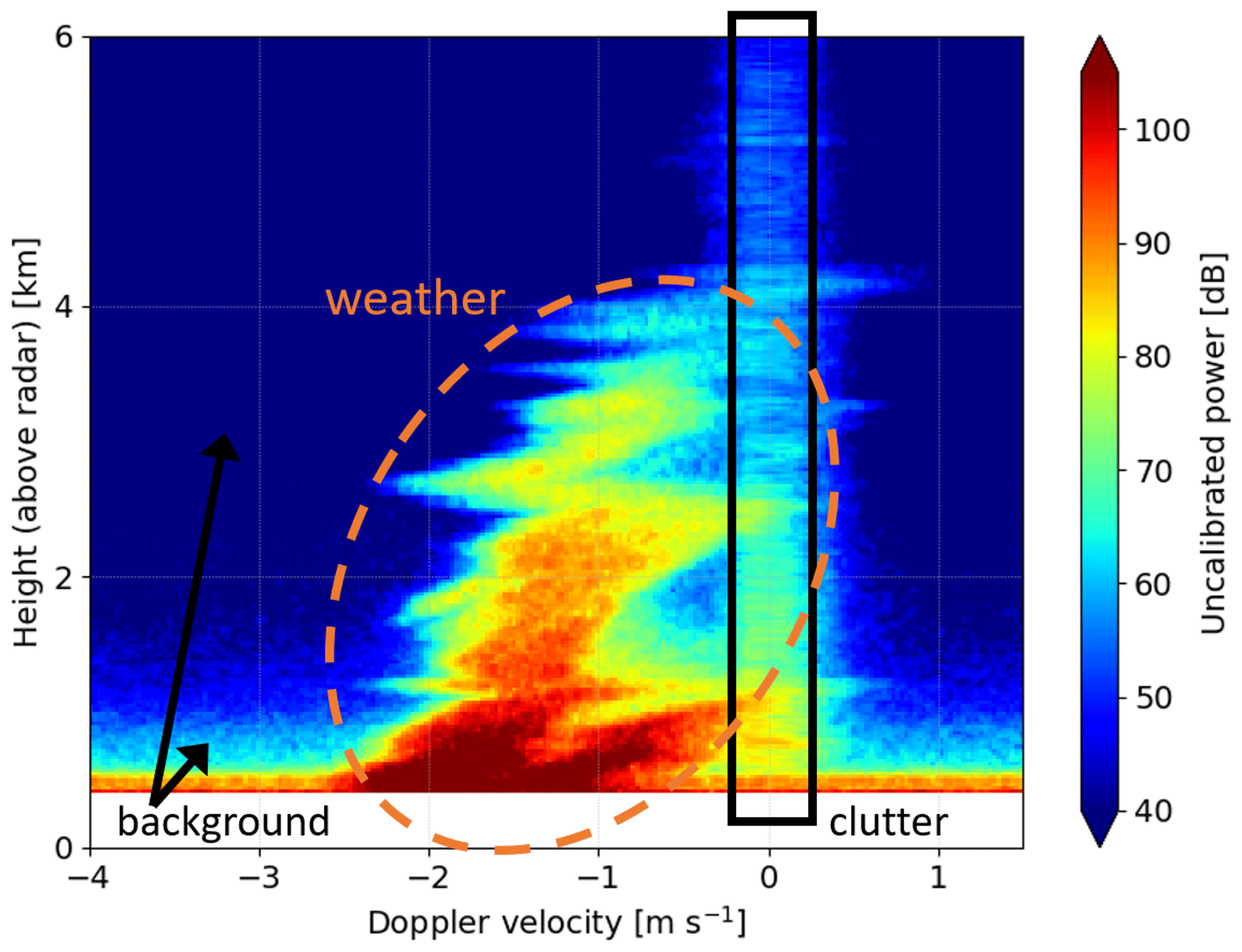
Figure 1 Profile of mean Doppler (power) spectra recorded with MOHp C-band radar in the H polarization channel in one birdbath scan during a snowstorm in the winter of 2020 (data timestamp: 18 January 2020, 00:24:46 UTC) after the internal radar signal processor had already applied a notch filter to mitigate strong clutter near 0 m s⁻¹ for each individual Doppler spectrum.

The birdbath scan spectral data that are summarized in Fig. 1 were collected at MOHp during the initial phase of a snowstorm in January 2020. At the time of these radar measurements, co-located in situ weather sensors recorded a rapidly falling near-surface temperature of 2.0 ^∘C and liquid equivalent precipitation rates at the ground of about 1 to 2 mm h⁻¹, together with wind gusts of up to about 8 m s⁻¹. According to atmospheric soundings derived from short-term predictions by the ICON atmospheric model (Zängl et al., 2015), the 0 ^∘C temperature is found at a height of about 0.2 km at the time of the measurement.

Figure 1 indicates that the weather signal caused by the precipitation and cloud particles is found below a height of about 4 km and at Doppler velocities between about −2.5 and 0 m s⁻¹. As the snow particles grow in size and mass, remitted power and particle fall speed generally increase from the cloud top toward the ground. The bimodal Doppler spectra with two distinct Doppler power peaks at heights below about 1 km make this an instructive test case for a detailed spectral analysis. In addition to the strong weather signal, static clutter at Doppler velocities near 0 m s⁻¹ along all heights, the antenna near field that extends up to a height of about 650 m across all Doppler velocities, and background noise around the fringes of the weather signal and at low heights all form non-negligible non-meteorological contributions to the overall radar signal. The following sections explain how these undesired non-meteorological contributions can be filtered from the radar data, how individual precipitation modes can be identified, and how modal and multimodal properties may then be calculated. A schematic overview of the analysis method is shown in Fig. 2.

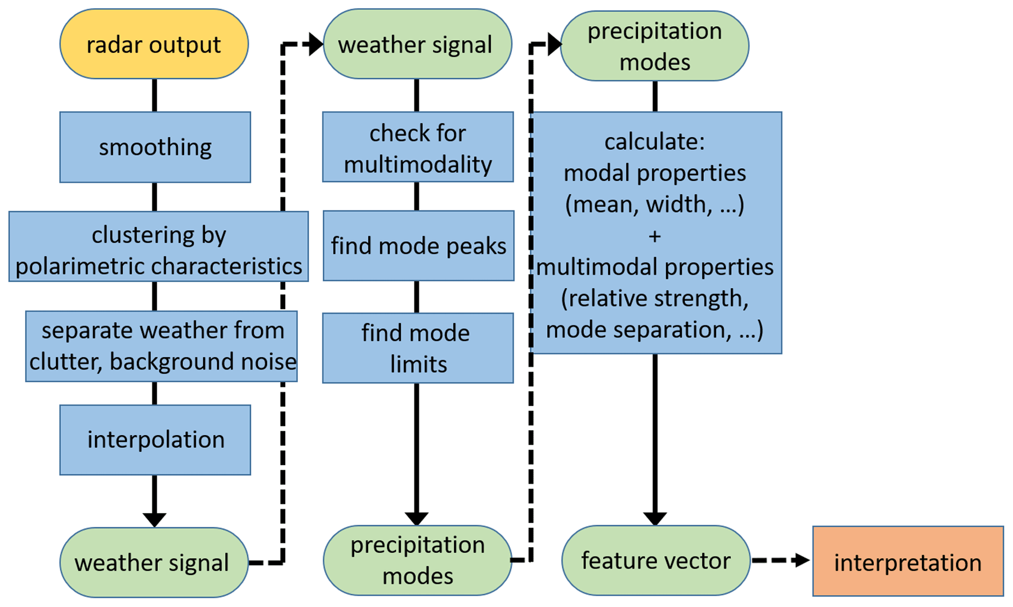
Figure 2 Outline of the proposed spectral postprocessing method. First, the weather signal is isolated from the non-meteorological contributions to the Doppler spectra (Sect. 2.2). Then, the precipitation modes are identified at each height (Sect. 2.3). Finally, quantitative characteristics of the precipitation modes are calculated, including uncertainty estimates, and can be collected in a feature vector to analyze the observed precipitation event (Sect. 2.4).

2.2 Weather signal

Some radar systems, particularly high-frequency cloud radars operated with fixed (i.e., non-rotating) antenna, show more benign clutter characteristics than DWD's C-band weather radars as illustrated in Fig. 1. For those cloud radars, the weather signal can be readily extracted from the radar output by assigning a simple power threshold level that roughly separates meteorological contributions to the Doppler spectra from the low-power background (Kollias et al., 2007).

When strong clutter is observed in the radar Doppler spectra, previously applied methods to exclude clutter contributions near Doppler velocities of 0 m s⁻¹ are commonly based on notch filters where the signal in a narrow prescribed velocity range around 0 m s⁻¹ is blanked out and the remaining signal is interpolated across the blanked-out range. However, this requires well-defined clutter characteristics across all measurements, which is not the case for DWD's weather radars and radar scan strategy. Figure 1 shows an example after already applying such a notch filter, which is performed automatically by the internal radar signal processor before the Doppler spectra are saved. A more refined approach has recently identified stationary ground clutter at 0 m s⁻¹ by evaluating how much the spectral power drops from the clutter maximum to neighboring velocity bins and by then comparing those values to the mostly smaller drop-off from power peaks attributed to precipitation instead of clutter (Williams et al., 2018). The power thresholds determined by this approach, however, can be rather specific to each analyzed precipitation event and did not show consistent results and sufficient flexibility in tests with DWD's C-band radar at MOHp.

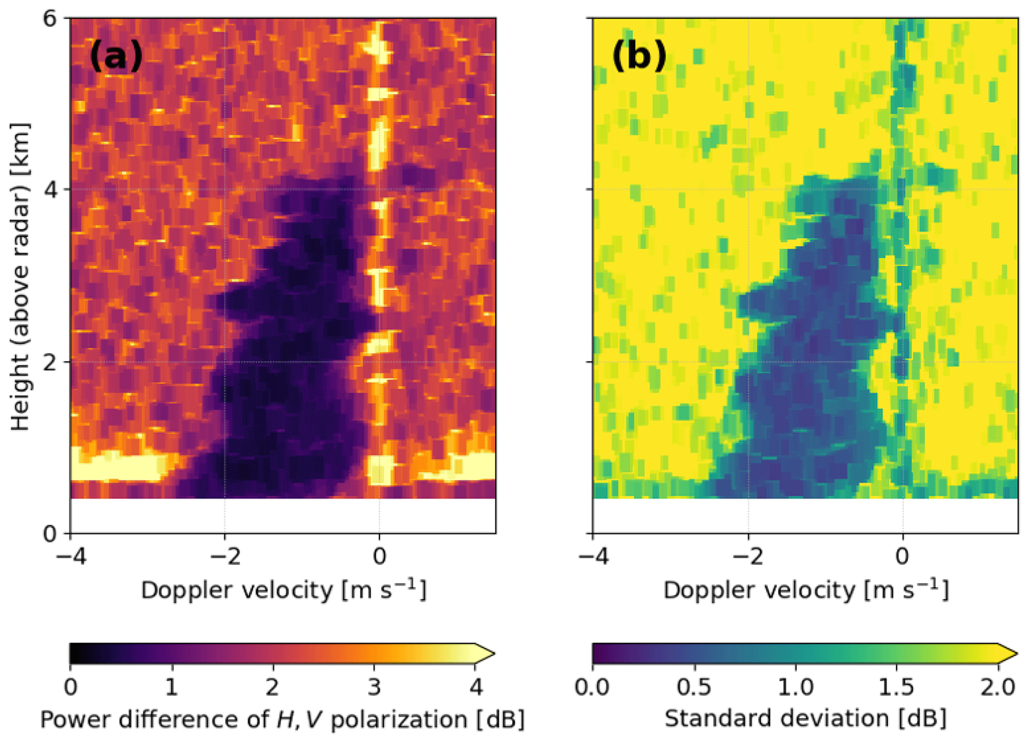
This study instead exploits differences in the polarimetric characteristics of precipitation and non-meteorological contributions to isolate the weather signal in the radar output of each birdbath scan. While precipitation particles are often preferentially oriented relative to the horizontal plane, e.g., dendritic snow often falls with the long axes oriented parallel to or at small canting angles to the horizontal plane, they are (azimuthally) randomly oriented within the horizontal plane (e.g., Matrosov et al., 2005). For vertically pointing radars, the signal power in the two orthogonal H and V polarization channels then shows only minor differences. Additionally, the signal is expected to change gradually with rather smooth transitions between adjacent Doppler velocity bins, because precipitation particle populations are generally assumed to be described adequately by smooth size distributions that translate to smooth fall speed distributions (e.g., Yuter et al., 2006; Petty and Huang, 2011; Gergely, 2019). Non-meteorological contributions to the radar signal, on the other hand, should show either significant differences between the two polarization channels, because the reflecting objects are preferentially oriented (e.g., a rigid strut in the radar beam of the antenna), or they lead to steep changes in received power for neighboring Doppler velocity bins (e.g., salt-and-pepper noise). To capture these polarimetric characteristics in the overall radar signal, three parameters are defined for each height and Doppler velocity bin: (i) the signal power in one of the polarization channels (here, the H channel as illustrated in Fig. 1), (ii) the absolute difference in signal power between both polarizations (i.e., the absolute value of the uncalibrated spectral differential reflectivity sZ_DR,u), and (iii) the standard deviation of signal strength differences between both polarization channels within a small neighborhood of Doppler velocities (which quantifies the texture of sZ_DR,u).

Here, the texture parameter (iii) is very similar to the texture parameter of the spectrally decomposed differential reflectivity used by Moisseev and Chandrasekar (2009) for filtering clutter and noise in polarimetric Doppler radar measurements that are collected at low elevation angles. Moisseev and Chandrasekar (2009) also exploited the cross spectra to compute the spectrally decomposed copolar correlation coefficient and the texture of the spectral differential phase as additional parameters for their polarimetric spectral filter. For DWD's vertically pointing birdbath scans, this study instead includes the sZ_DR,u absolute values in parameter (ii) to help identify non-meteorological contributions to the Doppler spectra.

To mitigate the bin-to-bin variance in the calculated polarimetric parameters (ii) and (iii), after averaging over the 15 Doppler spectra recorded during each birdbath scan, they are processed further by performing morphological grayscale closing across the entire Doppler velocity and height ranges with a structure element of a size of 7 Doppler velocity bins (∼0.2 m s⁻¹) and 3 height bins (75 m), using the ndimage.grey_closing() implementation provided in SciPy (Virtanen et al., 2020). Morphological closing was chosen specifically for smoothing occasionally deep spurious minima encountered inside regions of higher pixel values, analogous to filling small holes in binary black-and-white images. For the dimensions of the structure element, the length of seven Doppler velocity bins reflects the typical clutter range around 0 m s⁻¹, and three height bins represent the smallest interval that is symmetric about the center bin and ensures filling of spurious minima. Tests showed that the exact choice of the dimensions of the structure element usually has only a small impact on the results as long as it can approximately cover the Doppler velocity range of the static clutter around 0 m s⁻¹. Our choice is a compromise between smoothing over spurious data and still resolving small-scale meteorological features in the weather signal.

Figure 3 shows the results of the polarimetric parameters corresponding to Fig. 1. Static clutter at 0 m s⁻¹ is often marked by high differences in signal strength between the two polarization channels, the transition region from clutter or weather signal to the background are characterized by a high variability. Isolating the weather signal from all non-meteorological contributions then requires finding appropriate thresholds for both polarimetric parameters. Instead of manually determining two values that yield an adequate segmentation of all data collected for each birdbath scan by trial and error, the presented algorithm identifies appropriate thresholds by clustering the radar data defined in parameters (i) to (iii) and illustrated in Figs. 1 and 3, thereby emphasizing automation and flexibility.

Figure 3 Summary of polarimetric parameters corresponding to Fig. 1, as defined in Sect. 2.2: (a) absolute difference between the two polarization channels and (b) variability expressed through the standard deviation of the differences between both polarization channels within a small neighborhood.

While clustering algorithms have already been applied to polarimetric radar measurements to classify the observed precipitation types (e.g., Besic et al., 2016), to our knowledge, the use of clustering techniques for signal processing has not been explored. Here, a clustering algorithm is needed that can handle large datasets of ∼10⁶ individual data points per birdbath scan across all heights and Doppler velocities and that can cope with noisy data without blowing up due to extreme outliers in the dataset. The clustering algorithms currently implemented in the popular scikit-learn Python package did not meet these requirements (Pedregosa et al., 2011). Instead, the hierarchical density-based HDBSCAN clustering algorithm proved to be a flexible and scalable solution for clustering our radar data (Campello et al., 2013; McInnes et al., 2017). HDBSCAN is a density-based clustering algorithm that identifies data clusters based on their persistence in the clustering hierarchy. The algorithm was specifically developed to find clusters of varying density, size, and shape in large sets of multidimensional data including noise, without designating the number of expected data clusters a priori. These characteristics allow an application to diverse data without requiring extensive preprocessing. For this analysis, the three full datasets underlying Figs. 1 and 3 were merely rescaled to a maximum value of 1 to account for the often much higher numerical values of signal power than of the two polarimetric parameters.

The clustering results are illustrated in Fig. 4. The core of the weather signal that is required for further analysis is the narrow elongated cluster at small values of the polarimetric parameters. This (red) cluster contains 1.3 % of all data points. The (brown and purple) clusters at low signal power indicate the background signal and contain over 90 % of the data. The remaining (blue, orange, and green) clusters at medium to high signal power combined with relatively high polarimetric parameter values indicate different types of clutter and are formed by about 1 % of all data points. About 5 % of the data are not assigned to any cluster (indicated in black). In contrast to the cluster analysis of shallow snow clouds shown in Fig. 4, the core of the weather signal can cover a much higher percentage of Doppler velocity and height bins at the expense of the background signal for birdbath scans collected in precipitation where the clouds form at a higher altitude and where the particle fall speeds extend across a wider range of Doppler velocities, e.g., for stratiform rain analyzed in Sect. 3.

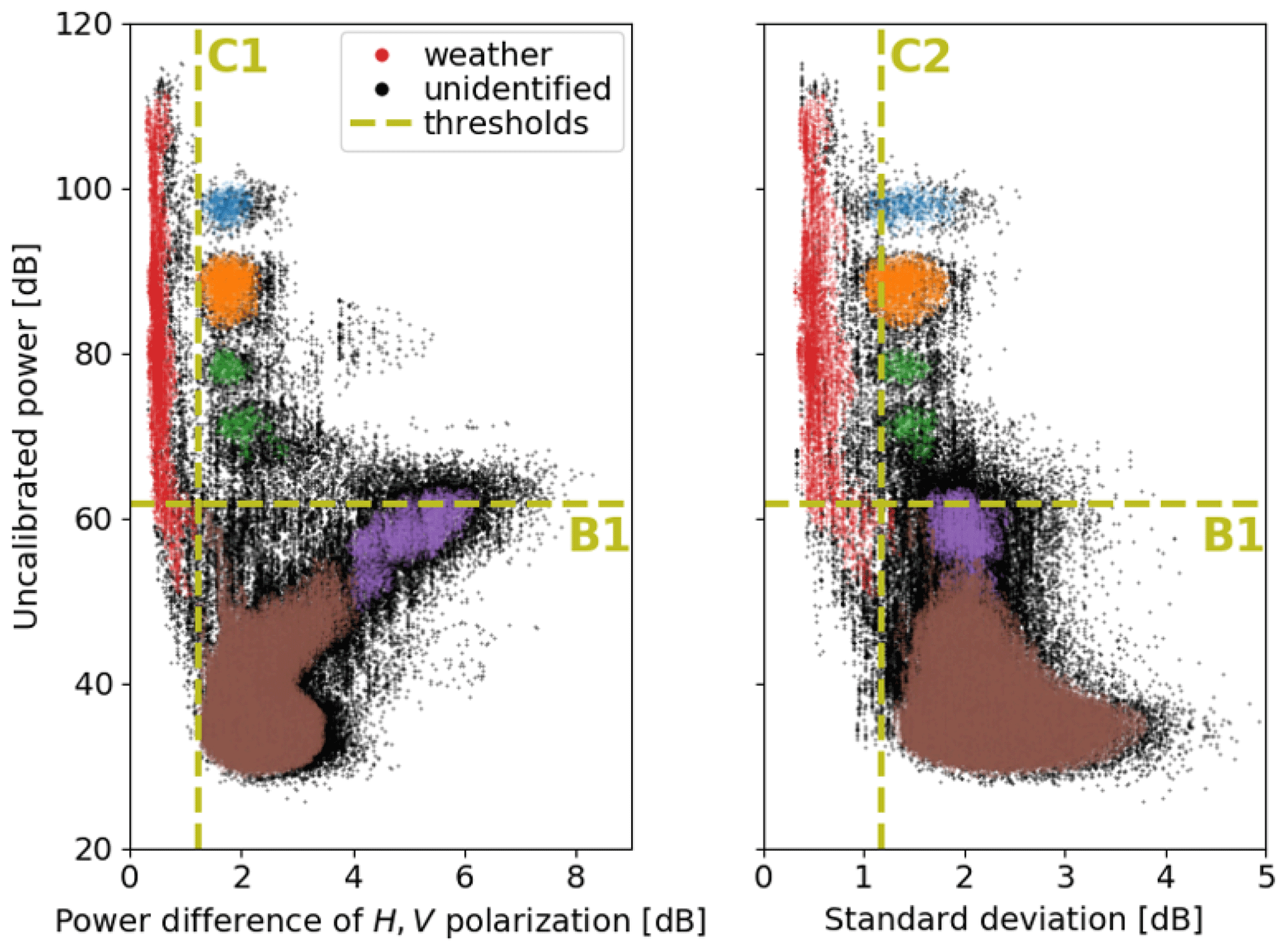
Figure 4 HDBSCAN cluster analysis of the Doppler spectra summarized in Fig. 1 and the two polarimetric parameters shown in Fig. 3. Colored regions indicate the clusters identified by HDBSCAN, and black dots mark data points that could not be assigned confidently by HDBSCAN to any of the clusters. Dashed olive lines give automatically determined thresholds (C1, C2, B1 as defined in the text), separating the core of the weather signal (red dots) from the other clusters that represent different non-meteorological contributions to the overall radar output.

The clustering results are used for implementing an automated thresholding method, which proved to deliver a stable segmentation of the data across many analyzed birdbath scans. Although cluster sizes and even the overall number of identified clusters can vary substantially, the defining properties remained consistent across the analyzed birdbath scans: the weather signal is characterized by small polarimetric parameters, the background signal by low Doppler powers, and the clutter signal by high Doppler powers and polarimetric parameters.

To separate the weather signal from clutter in Fig. 4, we choose the midpoints C1 and C2 between two characteristic x-axis values in both panels: (x1) the maximum x value of all data points that form the (red) cluster with the smallest quadratic sum of mean x values (i.e., the cluster with $min\left[{\mathrm{mean}}^{\mathrm{2}}\left(\mathrm{difference}\right)+{\mathrm{mean}}^{\mathrm{2}}\left(\mathrm{standard}\mathrm{deviation}\right)\right]$, which is the core weather signal) and (x2) the minimum x value of all data points in the (blue) cluster with the highest mean y value (i.e., the cluster with max[mean(uncalibrated power)], which is the strongest clutter signal). Similarly, the weather signal is separated from the low-power background signal by calculating the midpoint B1 between two characteristic y-axis values: (y1) the minimum y value of the core weather dataset colored in red and (y2) the maximum y value of the (brown) cluster with the lowest mean y value. If this y-value midpoint is smaller than the value determined for (y2), which is the case here because the y values of the red and brown clusters overlap, the value of (y2) is chosen for B1 instead to ensure that as much of the background signal as possible is excluded from further analysis. The final thresholds of C1=1.2 dB, C2=1.2 dB, and B1=62 dB are included in Fig. 4 as vertical and horizontal lines.

This thresholding algorithm can produce small data gaps in the filtered profile of mean Doppler spectra (i.e., filtered Fig. 1), e.g., when red data points fall below the threshold B1 in Fig. 4. Such data gaps are then filled via two-dimensional linear interpolation in dB space, with the limits of the interpolation interval once again given by the dimensions of the previously defined structure element. The idea here is that using the same structure element for morphological closing before identifying the clutter region and for interpolation afterward allows for estimating the weather signal across the clutter region. If the weather signal extends sufficiently into the clutter region, this approach prevents a loss of the contributions of the weather signal within the clutter region altogether, similar to the interpolation on a finer velocity scale presented by Williams et al. (2018). The weather signal is thus finally extracted from the original profile of mean Doppler spectra in the H polarization channel and shown in Fig. 5a.

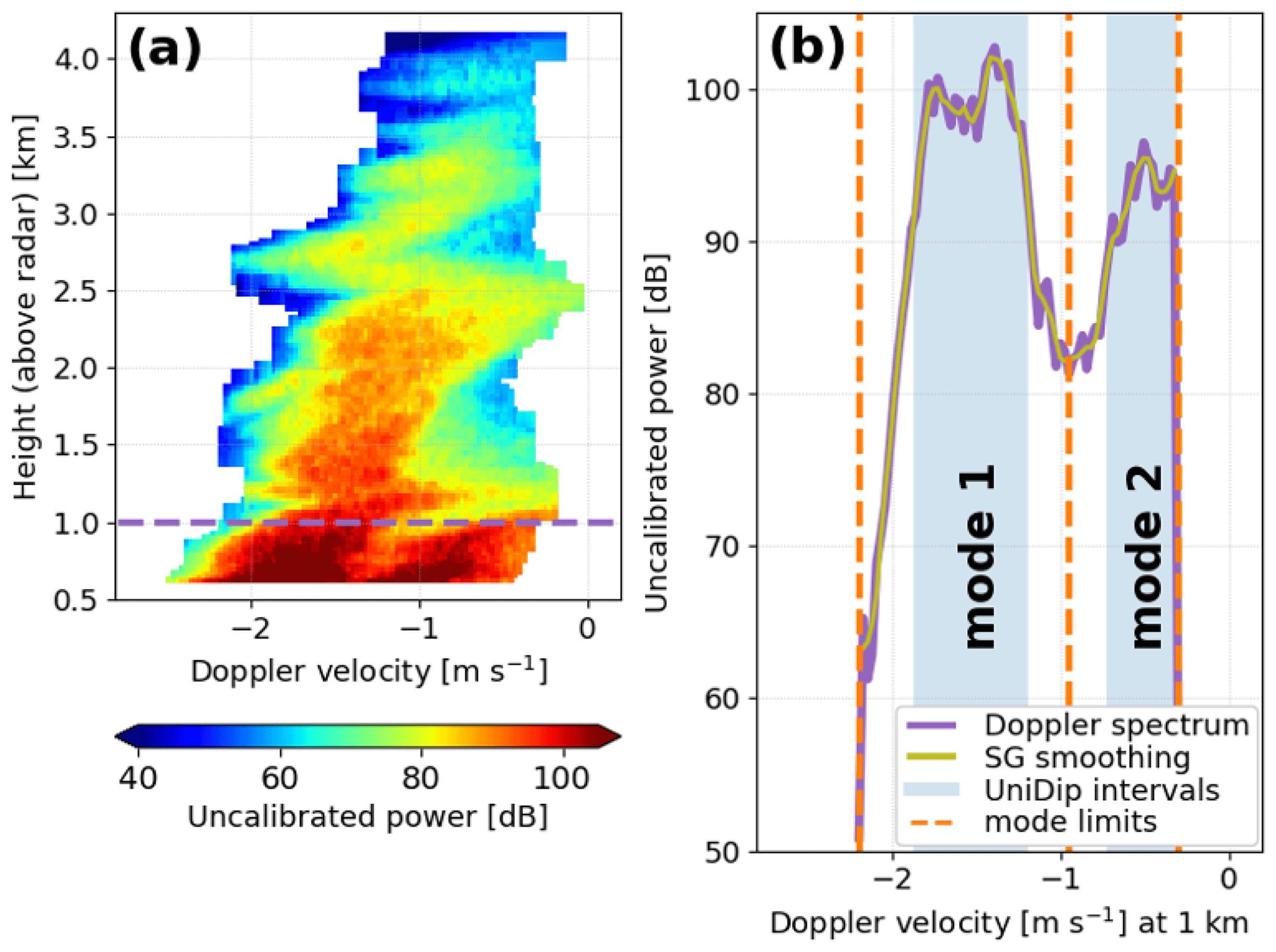
Figure 5 (a) Isolated weather signal after postprocessing as explained in Sect. 2.2; the horizontal dashed line at 1 km height indicates (b) one example of a bimodal Doppler spectrum. The UniDip clustering algorithm is used to identify statistically significant precipitation modes after smoothing the Doppler spectrum with a second-order Savitzky–Golay (SG) filter.

In Fig. 5a, interpolation accounts for only 5.7 % of the entire isolated weather signal, or for 483 pixels where each pixel corresponds to a unique combination of height and velocity bins. The median area of the interpolated regions is 9 pixels, and the median power of all interpolated pixels is 57 dB, which is still below the automatically identified power threshold of B1=62 dB that separates the core weather signal from the background in Fig. 4. Consequently, the interpolation procedure only contributes to the analysis by filling small gaps in regions of low Doppler power that are located mostly at the fringes of the weather signal in Fig. 5a. Particularly inside the melting layer of stratiform precipitation and in intense precipitation, the automatic thresholding method for filtering out the non-meteorological contributions to the Doppler spectra can lead to much larger gaps also in the high-power regions of the weather signal. The subsequent interpolation is then needed to close more substantial gaps in regions with much higher Doppler powers. In such cases, the two-dimensional interpolation employed here introduces artifacts that can strongly impact the further quantitative analysis of the Doppler spectra.

The presented automated postprocessing chain relies only on general characteristics of the radar data without making manual choices specific to each radar observation. Therefore, this methodology should not break down due to small variations in radar performance across a radar network. In Sect. 3, the same algorithm is applied for different DWD C-band radars, and the impact of different precipitation conditions on the results is evaluated, e.g., stratiform precipitation and intense frontal showers.

2.3 Precipitation modes

After isolating the weather signal, the precipitation modes contained in every Doppler spectrum can be identified. The current go-to solution of assigning a predetermined threshold value to identify precipitation modes in a Doppler spectrum, e.g., by requiring a minimum Doppler peak prominence or width for any additional mode to be recognized as such, limits the analysis to cases that do not deviate too far from these prescribed conditions (Kollias et al., 2007; Williams et al., 2018). Other radar noise-filtering algorithms that could potentially be adopted to find precipitation modes in noisy Doppler spectra similarly rely on fixed power thresholds for detecting peaks in the radar signal and offer only limited flexibility for analyzing the large variety of Doppler signals in different precipitation events (e.g., the GMAP algorithm presented by Siggia and Passarelli, 2004, assumes a unimodal weather signal a priori, in contrast to the bimodal weather signal analyzed in Sect. 2.2, and presupposes that the shape of the signal can be adequately parameterized as a Gaussian).

This study instead explores a novel, more adaptive method for identifying statistically significant peaks in every Doppler spectrum within the isolated weather signal by applying the univariate component UniDip of the multivariate SkinnyDip clustering algorithm (Maurus and Plant, 2016). The UniDip clustering algorithm finds clusters, i.e., regions of local maxima (or modes) for a univariate distribution, by repeatedly applying the nonparametric dip test. The dip test checks the given distribution for multimodality by exploiting the shape of the cumulative distribution function (Hartigan and Hartigan, 1985): a local maximum leads to a change in the shape of the cumulative distribution function from a convex form up to the mode to a concave form after the mode, independent of the specific parameterization or shape of the underlying distribution. UniDip is particularly well suited for analyzing noisy data and determines all statistically significant modes based on the noise characteristics of the data distribution and the desired significance level. Here, a significance level of p≤0.05 is chosen, which is commonly used in statistical hypothesis testing and corresponds to a confidence level of 95 %.

Figure 5b shows an example Doppler spectrum at a height of 1 km above the radar. First, the Doppler spectrum is smoothed with a second-order Savitzky–Golay (SG) filter, using a smoothing window length of seven Doppler velocity bins that was already used in Sect. 2.2 (Savitzky and Golay, 1964; Virtanen et al., 2020). This filtering step leads to more gradual transitions in the Doppler spectra without sharp signal spikes, and choosing a second-order SG filter still allows the filtered spectra to follow the outline of signal peaks better than a simple moving average filter, for example. Additionally, the differences between SG-filtered and SG-unfiltered Doppler spectra will be used later on to estimate uncertainties in the quantitative characteristics of the precipitation modes that are calculated in Sect. 2.4.

Interpreting each SG-filtered Doppler spectrum within the isolated weather signal as a frequency distribution of Doppler velocities, a discrete distribution of Doppler velocity samples is generated according to the Doppler power in each bin. The UniDip algorithm can then be applied to the generated distribution to identify clusters of Doppler velocities. The UniDip outputs are estimates of the statistically significant modal intervals in each Doppler spectrum, illustrated by the lightly shaded regions in Fig. 5b. As the modal intervals determined by UniDip do not capture the full weather signal, we only use the UniDip outputs to identify the highest Doppler power in each interval, which is then interpreted as the Doppler peak of each precipitation mode. The UniDip algorithm is thus essentially utilized for finding the relevant Doppler peaks without having to specify either the peak prominence or the separation between two peaks.

The start or end point of each precipitation mode is either assigned to the Doppler velocity bin forming one of the two edges of the weather signal, the Doppler velocity corresponding to the minimum between two adjacent peaks, or the Doppler velocity where the Doppler spectrum first dips below the noise power level when moving away from the peak power. Here, the noise level is defined as the median Doppler power of all velocity bins that fall outside the weather signal, i.e., the non-meteorological contributions to the radar output at the same height level that were filtered out according to Sect. 2.2. This approach provides a robust noise estimate, because the high clutter power that is found only within a narrow velocity range has no notable impact on the median power of all velocity bins outside the weather signal. In Fig. 5b, the resulting mode limits are indicated by vertical dashed lines and specify the two individual precipitation modes (in this example) required for the quantitative analysis in the next section.

Using the UniDip clustering algorithm to identify the precipitation modes in the weather signal leads to consistent results across different precipitation conditions, without having to manually adjust any preset parameters. The proposed method also does not require the Doppler spectra to be of any specific shape or the modes to follow any specific parameterization such as a Gaussian.

2.4 Quantitative characteristics

Similar to previous studies that analyzed Doppler spectra from higher-frequency cloud radars (Kollias et al., 2007; Maahn and Löhnert, 2017; Williams et al., 2018), this study includes calculations of the zeroth- to fourth-order moments of the individual precipitation modes that were identified following Sect. 2.3. Here, the equations presented by Williams et al. (2018) are adapted to the spectral output of DWD's C-band weather radars that is given as uncalibrated power. Additionally, the metric of “median skewness” is calculated as an alternative measure of the asymmetry of a precipitation mode, and several multimodal properties are introduced following Zhang et al. (2003) to specify the relation between individual modes whenever multiple precipitation modes are identified in a single Doppler spectrum. Furthermore, uncertainty estimates are derived for all calculated quantitative characteristics. The equations used for calculating the modal and multimodal properties that are discussed here are listed in Appendix A.

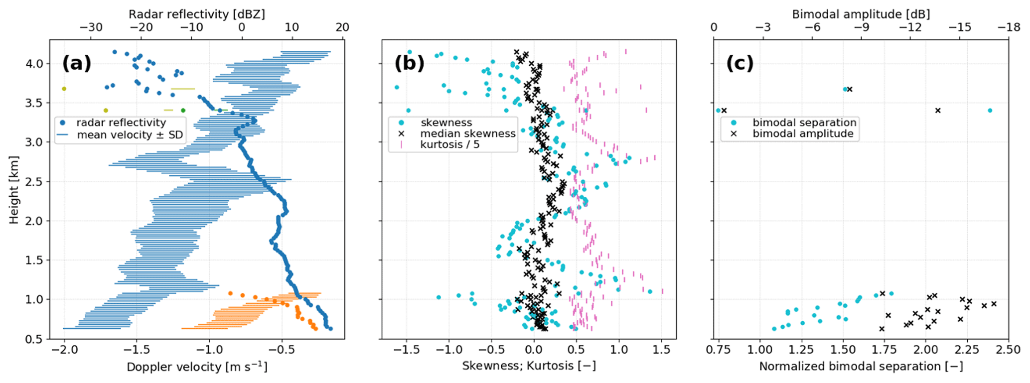
Figure 6 Summary of (a, b) modal and (c) multimodal properties calculated for all Doppler spectra that form the weather signal shown in Fig. 5a. Different colors in panel (a) indicate different precipitation modes that are identified following the methodology presented in Sect. 2.3; in panels (b) and (c), different modes are not marked by different colors.

Figure 7 Uncertainty estimates for all data shown in Fig. 6. Corresponding mean and median values are listed in Table 2.

Figures 6 and 7 summarize the results for the test case considered throughout Sect. 2.1 to 2.3. Figure 6a quantifies the bimodality in the Doppler spectra at heights of about 1 km and below that was already observed in Figs. 1 and 5. The main precipitation mode forms above a height of 4 km. While the frozen precipitation particles fall toward the ground and grow in mass and size, the radar reflectivity increases to Z_H=18 dBZ. Simultaneously, the core snowfall signal, marked by the range of mean Doppler velocity ($\stackrel{\mathrm{‾}}{v}$) ± the standard deviation (SD), shifts toward more negative values of $v<-\mathrm{1.5}$ m s⁻¹, which can be interpreted as a strong increase in the typical particle fall velocity. Just above 1 km, a second precipitation mode develops. The particles in this secondary precipitation mode exhibit slower typical fall velocities, given by Doppler velocities of $v>-\mathrm{1.2}$ m s⁻¹, and the radar reflectivity, while sharply increasing toward the ground, still remains below the reflectivity of the primary precipitation mode. Results calculated for two Doppler spectra around a height of 3.5 km also suggest the existence of multiple precipitation modes at these altitudes (green markers in the top part of Fig. 6a). But, an exact interpretation of the analysis results at these weak radar reflectivities below 0 dBZ is difficult due to the generally higher associated uncertainties (see also the discussion of Fig. 7 below). Nonetheless, a detailed comparison with the radar output data and the isolated weather signal indicates that the multimodality here is introduced artificially by the two-dimensional interpolation during postprocessing, as described in Sect. 2.2.

Figure 6b shows the corresponding modal properties of skewness and kurtosis. These higher-order Doppler moments are very sensitive to spectral broadening, which is seen by the sharply higher values at heights of just above 1 km and at 2.5 to 3 km. At low radar reflectivities above about 3.5 km, skewness and kurtosis also show strong deviations from 0. The median skewness is less affected by spectral broadening and thus by atmospheric air movements due to turbulence, therefore potentially offering a more stable alternative for quantifying the asymmetry of a precipitation mode than the moment of skewness. However, the decreased sensitivity also means that the overall dynamic range of the median skewness is rather compressed, and small variations in median skewness caused by actual precipitation processes may be difficult to interpret or even detect.

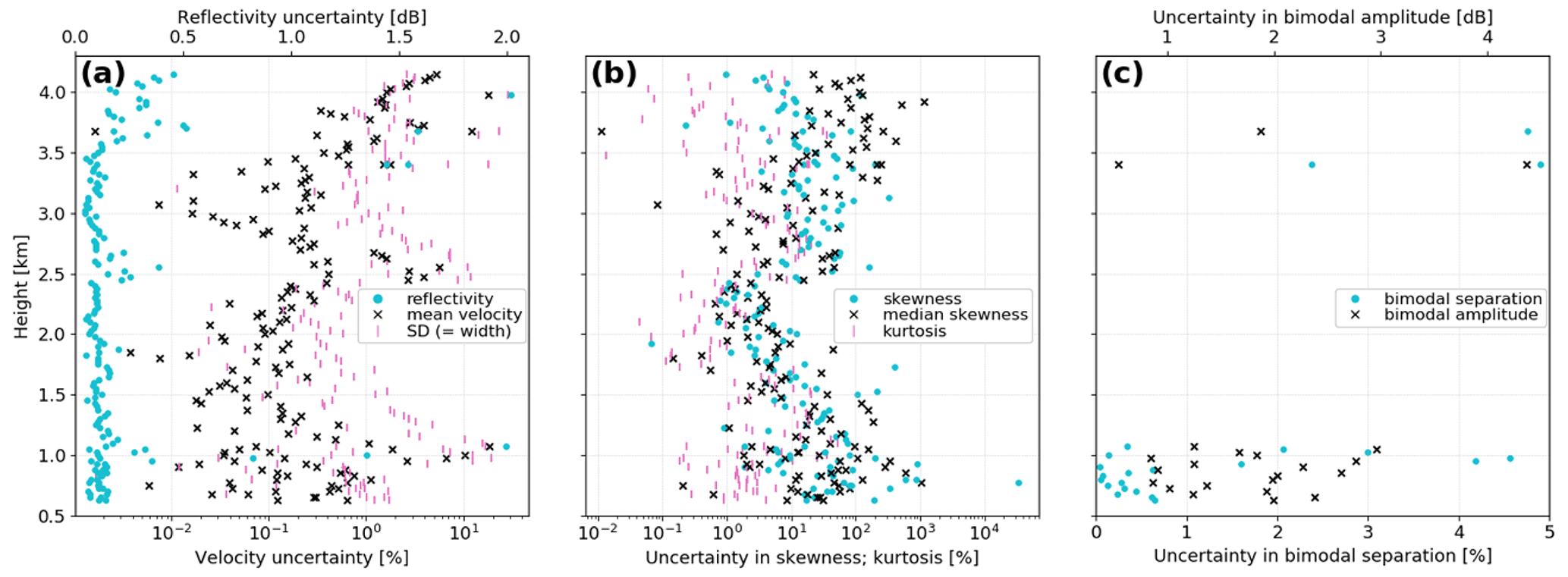
Table 2 Mean and median values of all uncertainty estimates shown in Fig. 7.

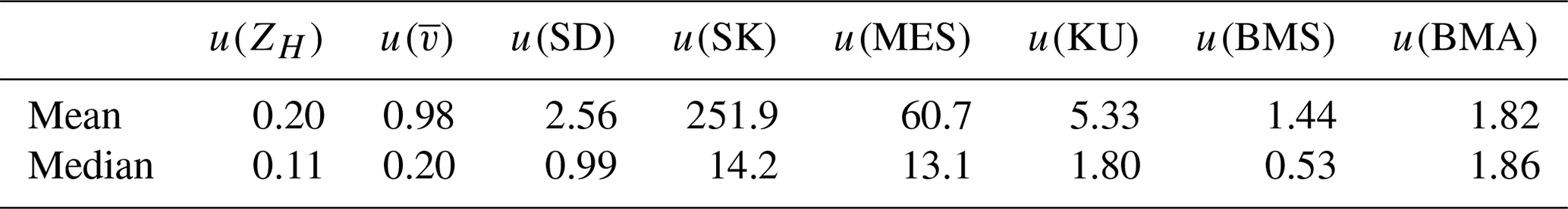
Relative uncertainties u for radar reflectivity Z_H and bimodal amplitude (BMA) are given as dB values; uncertainties for mean Doppler velocity $\stackrel{\mathrm{‾}}{v}$, standard deviation (SD), moment of skewness (SK), median skewness (MES), kurtosis (KU), and bimodal separation (BMS) are percentages.

Figure 6c illustrates two multimodal properties that were calculated for all multimodal Doppler spectra found in Fig. 6a. The bimodal separation indicates the distance between two precipitation modes, normalized by their standard deviations, and the bimodal amplitude quantifies the prominence of the smaller of the two mode peaks. These variables can help give a clearer picture of how the precipitation modes evolve than the modal properties in Fig. 6a and b alone.

In Fig. 6c, the decrease in bimodal separation from a height of 1 km downward illustrates the gradual convergence of both precipitation modes as the snow falls toward the ground. Conversely, the bimodal amplitude (BMA) does not follow such a clear trend. From the minima of BMA < −15 dB found just below 1 km, the bimodal amplitude increases both toward the ground and toward the heights where the secondary precipitation mode first forms. In the first stage of the generation of the secondary precipitation, the newly forming precipitation mode found in the Doppler spectrum is still relatively weak compared to the overlapping signal of the much stronger primary precipitation that extends to these Doppler velocities. So the prominence of the secondary peak is still small here, and thus the bimodal amplitude is given by only moderately negative values. As the secondary precipitation matures rapidly, BMA values decrease sharply toward their minimum. After the secondary precipitation has fallen past the altitude marked by the BMA minimum, mixing between the two simultaneously occurring snowfall processes increases. Here, the secondary precipitation peak again becomes less distinct as a higher amount of snow can be characterized as falling “in between” the two pure precipitation modes, which is reflected in the increase in bimodal amplitude toward less extreme values near the ground.

Uncertainties in the modal and multimodal properties can be estimated by calculating the same properties with alternative inputs that reflect realistic assumptions about uncertainties associated with the radar observations and postprocessing method (e.g., by strictly following JCGM 100:2008, 2008). In this study, all spectral properties are calculated both for the SG-smoothed and SG-unsmoothed Doppler spectra (see Fig. 5), and the difference between the two results is then assumed to represent a simple uncertainty estimate. The motivation for using this approach is not to capture all effects that may propagate through the postprocessing chain and quantify them in detail. Instead, this uncertainty assessment aims at evaluating which modal and multimodal properties may be the most reliable for analyzing DWD's C-band radar Doppler spectra.

The uncertainty estimates shown in Fig. 7a and the corresponding averages listed in Table 2 suggest that the lower-order Doppler moments of radar reflectivity, mean velocity, and standard deviation are characterized by small relative uncertainties of generally less than 5 % (u(Z_H)=0.2 dB ∼ 5 %). Uncertainty maxima are mostly found at high altitudes where the radar signal is very weak (see Fig. 6a), a trend previously observed by Kollias et al. (2007). Uncertainty estimates for the kurtosis are also generally limited to 5 %–10 %, as illustrated in Fig. 7b. But both the moment of skewness and the median skewness show much higher uncertainties, including extreme values of much more than 100 %. For the multimodal properties, the bimodal separation is characterized by similarly small relative uncertainties as the lower-order Doppler moments, and the bimodal amplitude shows higher uncertainties of typically around 2 dB according to Table 2.

In summary, particularly the two skewness measures are highly sensitive to small variations in the Doppler spectra caused by atmospheric air movements like turbulence. To mitigate the impact of air movements and focus on only the spectral signatures of precipitation processes, the scanning strategy would need to be adjusted by recording and averaging Doppler spectra over a longer time period. This would ensure smoothing of rapid fluctuations in the Doppler spectra associated with turbulent air motion. The time constraints imposed by the operational scanning cycle, however, make such a modification of the birdbath scan difficult, besides examining individual test cases with modified scan settings outside of regular radar operations. Based on these findings, the analysis of Doppler spectra recorded by DWD's birdbath scans mostly focuses on the lower-order moments of radar reflectivity, mean velocity, and standard deviation, as well as on the multimodal property of bimodal separation whenever multiple precipitation modes are identified in a Doppler spectrum. Nonetheless, Sect. 3 also includes a snowfall example where only the skewness and kurtosis profiles show a distinctive feature that indicates the presence of a secondary precipitation process, which is not captured by the lower-order Doppler moments alone.

3 Results and discussion

In addition to the test case presented in the previous section, this section discusses the results of four birdbath scans collected at different DWD C-band radar sites across Germany and for varying precipitation conditions in 2021: snowfall in southern Germany, light rain off the German North Sea coast, stratiform rain in western Germany, and intense frontal rain in eastern Germany.

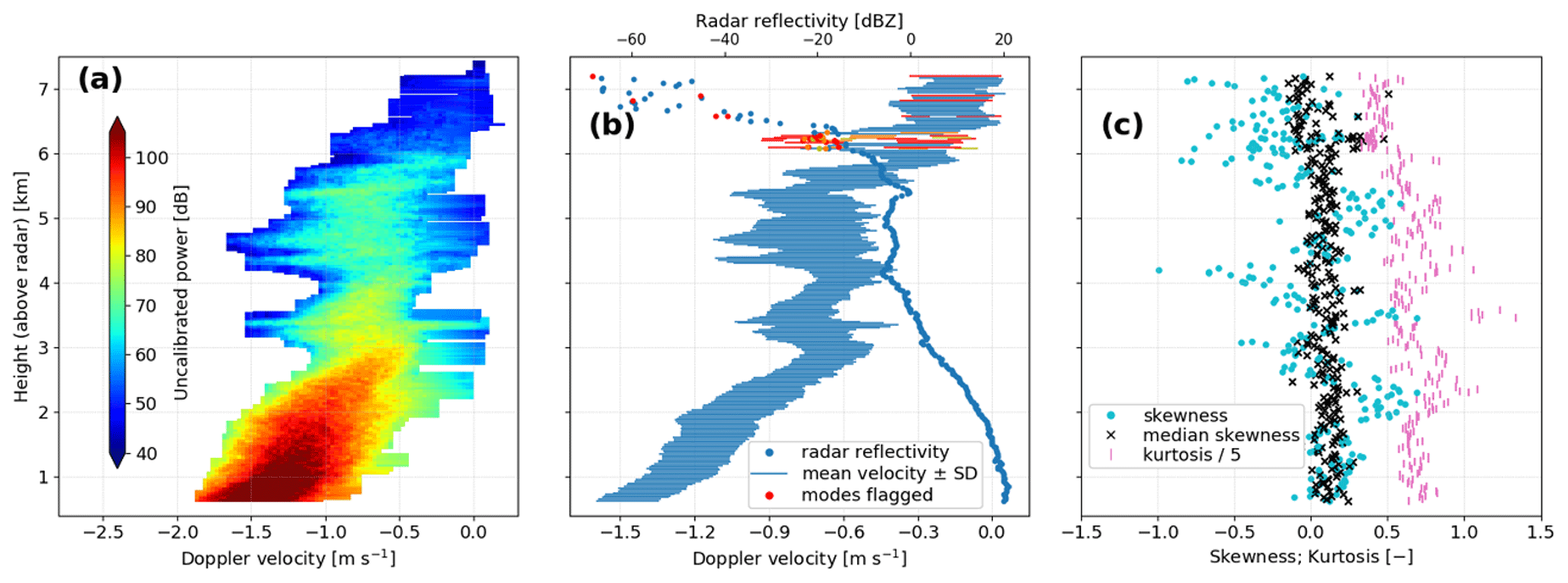
Figure 8 Summary of analysis results for a birdbath scan recorded at DWD's Isen (ISN) radar near Munich during a snowfall event in December 2021 (data timestamp: 9 December 2021, 06:04:12 UTC); (a) isolated weather signal analogous to Fig. 5a and (b) modal properties of lower-order and (c) higher-order Doppler moments corresponding to the test case at the MOHp radar shown in Fig. 6a and b, respectively.

Figure 8 summarizes the analysis results for the Doppler spectra recorded at the Isen (ISN) radar near Munich in one birdbath scan during a snowfall event (ISN radar lat: 48.174705^∘ N, long: 12.101779^∘ E; alt: 678 m a.s.l.). At the time of the birdbath scan, nearby in situ weather sensors showed a liquid equivalent precipitation rate of about 1 mm h⁻¹ and a temperature of just below 0 ^∘C as the snow clouds passed over the radar from the southwest with only weak near-surface winds of about 1 m s⁻¹. In contrast to the Doppler spectra that were discussed throughout Sect. 2 and collected during a snowfall event at MOHp, Fig. 8 indicates that this snowfall was characterized by only a single precipitation mode. Few multimodal spectra are identified near the cloud top, where the radar signal is very weak with a radar reflectivity of less than −10 dBZ. The corresponding modes have been flagged as erroneous results in Fig. 8b, because the multimodality here is likely an artifact introduced by the marginal quality of the weak radar signal.

The higher-order Doppler moments of skewness and kurtosis in Fig. 8c show a high sensitivity to spectral broadening, regardless of whether the spectral broadening is caused by precipitation processes or atmospheric turbulence, which was already observed in Sect. 2.4. Nonetheless, one meaningful feature can still be recognized at heights just above 2 km: here, both skewness and kurtosis are characterized by higher values than immediately above and below this altitude, which coincides with the Doppler spectra in Fig. 8a showing a small bump on the right side of the core weather signal toward slower Doppler velocities around −0.5 m s⁻¹. The bump is still not significant enough to be identified as a separate mode during postprocessing, but it does already clearly affect the calculated higher-order Doppler moments. Given the persistence over multiple birdbath scans, this feature likely indicates a secondary precipitation process that contributes to snow formation and growth below this altitude and is not merely due to turbulent air motion or introduced by the postprocessing algorithm.

The discussion of Fig. 8 then suggests that the higher-order Doppler moments can pick up precipitation characteristics that are not always evident in the radar reflectivity, mean Doppler velocity, and standard deviation alone when the spectral signatures are not yet clear enough to indicate two simultaneously occurring precipitation populations. This feature illustrates a potential benefit of including skewness and kurtosis in a spectral analysis, as already pointed out by Maahn and Löhnert (2017) for cloud radars, even if these higher-order moments can also be strongly affected by atmospheric air movements, as seen for the Doppler spectra from DWD's C-band radar birdbath scans.

To better quantify the precipitation processes that drive each snowfall event, the typical degree of riming can be evaluated for each identified precipitation mode. Kneifel and Moisseev (2020) derived polynomials for estimating the rime mass fraction (RMF) from the mean Doppler velocity at different radar frequencies. They did not determine a polynomial relationship for C-band frequencies explicitly, but our tests of several of their listed polynomials showed only a minor influence of the specific choice of frequency-dependent polynomial relationship once RMF≥0.15. To ensure a sensible range of retrieval results of RMF≳0 also for slow Doppler velocities, their X-band polynomial was chosen for this analysis. Additionally, RMF retrieval uncertainties are quantified in this study via the impact of normalizing every mean Doppler velocity to a standard surface pressure of 1000 mbar at MOHp. Kneifel and Moisseev (2020) suggest such a normalization before performing all riming retrievals, because their polynomials were derived for near-surface data, but here the required data are only available for our MOHp radar observations, where sounding data from short-term predictions by DWD's operational ICON atmospheric model can be used to estimate the atmospheric pressure profile (Zängl et al., 2015). The resulting retrieval uncertainties of generally 20 % to 30 % do not include effects due to vertical air motions that can shift the entire Doppler spectrum and thus the mean Doppler velocity substantially, particularly in strongly convective snowfall. Furthermore, Kneifel and Moisseev (2020) found a highly non-unique relation between mean Doppler velocity and RMF at slow fall velocities. These significant uncertainties in determining the rime mass fraction at slow fall velocities are also not captured by our approach for retrieving RMF.

RMF retrieval results for the two birdbath scans discussed so far are shown in Fig. 9. The fast-falling main mode in the MOHp snowfall example yields the highest retrieved rime mass fractions of RMF>0.5 near the ground, suggesting that riming is the dominant precipitation growth process in the lower part of the atmosphere during this birdbath scan. Kneifel and Moisseev (2020) used a threshold of retrieved RMF>0.5 to indicate a riming event and found overall median retrieved values of $\mathrm{0.5}\le \mathrm{RMF}\le \mathrm{0.6}$ for all riming events they identified at four CloudNet sites in central and northern Europe (Illingworth et al., 2007). In Fig. 9, precipitation particles in the weaker MOHp secondary mode appear to be much less affected by riming, implying that relatively pristine snow crystals or unrimed polycrystals occur simultaneously with the significantly rimed particles of the main precipitation mode.

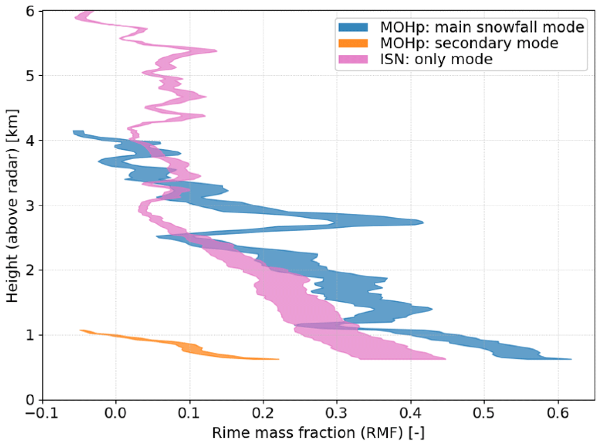
Figure 9 Retrieval of rime mass fraction (RMF) for both precipitation modes identified in the MOHp snowfall test case shown in Fig. 6a and for the only precipitation mode found in the example from the ISN radar shown in Fig. 8. Colored RMF ranges at each height reflect estimated retrieval uncertainties of generally 20 % to 30 %.

The supply of supercooled liquid water that is required for riming of the frozen precipitation particles cannot be identified in the C-band radar Doppler spectra shown in Figs. 1, 5, and 6. These small liquid drops are characterized by Doppler velocities close to 0 m s⁻¹ and only cause a weak radar echo compared to the much higher signal strengths of the larger precipitation particles and the static clutter near 0 m s⁻¹. Some cloud radars with more benign clutter characteristics instead offer the necessary sensitivity to directly identify the supercooled liquid water associated with riming in their high-resolution Doppler spectra (e.g., Kalesse et al., 2016). Nonetheless, our results suggest that C-band radar Doppler spectra can still be used to identify multiple simultaneously occurring precipitation modes (with sufficiently strong radar echoes) and allow for a granular analysis of riming by quantifying the degree of riming based on the typical fall velocity of each precipitation mode.

According to Fig. 9, the snowfall data recorded by the ISN radar show a gradual increase in retrieved rime mass fraction toward the ground with maximum values of RMF≈0.4. Combined with the higher radar reflectivity of up to 20 dBZ near the ground and the slightly lower in situ precipitation rates compared to the MOHp snowfall example, the RMF retrievals suggest that the ISN snowfall event contained larger snow particles with a lower mass density and was thus driven by aggregation as the dominant snow particle growth mechanism. This conclusion is also corroborated by the much slower near-surface wind speeds close to the detection limit of the wind sensor that were observed for the ISN snowfall event, implying calm atmospheric conditions that are beneficial for more undisturbed snowflake growth by aggregation.

The birdbath scan strategy and radar postprocessing method were initially developed to investigate frozen and mixed-phase precipitation above the melting layer in detail. But the analysis can also be applied to other precipitation conditions. Several examples are discussed in the following paragraphs, with an emphasis on the challenges posed by the melting layer and strong convective precipitation.

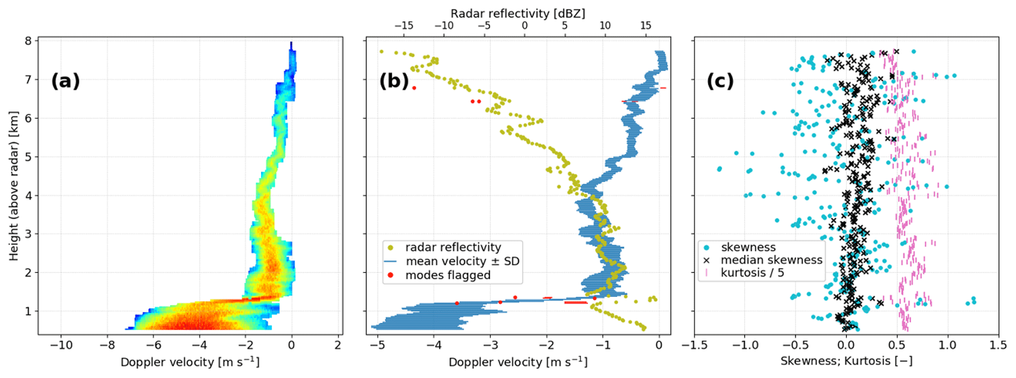
Figure 10 Summary of analysis results for a birdbath scan recorded in light rain at DWD's Borkum (ASB) radar in April 2021 (data timestamp: 29 April 2021, 14:14:12 UTC), analogous to Fig. 8 but with different scaling of x and y axes.

Figure 10 shows the results for a birdbath scan recorded by the Borkum (ASB) radar off the German North Sea coast in the spring of 2021 (ASB radar lat: 53.564131^∘ N, long: 6.748317^∘ E; alt: 36 m a.s.l.). For the time of the radar measurement, in situ weather data collected on Borkum island indicate very light rain of about 0.5 mm h⁻¹ and a near-surface temperature of 9 ^∘C. Figure 10a nicely illustrates the transition from (slow-falling) frozen precipitation to much faster-falling rain at heights around 1.3 km above the radar. At these heights, Fig. 10b also indicates a sharp spike in radar reflectivity, often called the radar bright band that is associated with the partial melting of frozen precipitation particles so that they are still larger than rain drops but their surface is already covered by liquid water (e.g., Ryzhkov and Zrnic, 2019). Below the melting layer, the precipitation falls toward the ground as rain, characterized by a higher fall velocity and a wider distribution of fall velocities (with mean Doppler velocities of about −4 m s⁻¹ below the melting layer vs. −1 m s⁻¹ above, and standard deviations of about 0.8 m s⁻¹ below vs. 0.3 m s⁻¹ above). The presence of such a clearly formed radar bright band and a simultaneous strong increase in precipitation particle fall velocity across a narrow melting layer points to relatively calm atmospheric conditions with little convection at the time of the birdbath scan.

Apart from two Doppler spectra at high altitudes, where the signal is very weak, the only Doppler spectra where the postprocessing algorithm presented in Sect. 2 indicates the existence of multiple precipitation modes are found within the melting layer in Fig. 10b. Inside the melting layer, the radar Doppler signal of the precipitation shows similar polarimetric characteristics as the clutter signal, i.e., a strong Doppler power and a higher difference and variability in the polarimetric parameters that are used to isolate the weather signal from clutter and background noise as outlined in Sect. 2.2. This behavior leads to more incomplete Doppler spectra inside the melting layer and then requires more extensive interpolation than for precipitation above and below the melting layer. The need for more substantial interpolation can introduce artifacts in the Doppler spectra and results in erroneously identifying the corresponding Doppler velocity interval as a separate precipitation mode. These modes generally also exhibit unrealistically low radar reflectivities inside the bright band and are therefore flagged as artifacts. Similarly, the only prominent feature that can be observed in the higher-order Doppler moments plotted in Fig. 10c is a spike inside the radar bright band. Given the more extensive interpolation inside the radar bright band, a detailed interpretation of skewness and kurtosis in the melting layer is also difficult.

Figure 11 Summary of analysis results for a birdbath scan recorded in stratiform rain at DWD's Essen (ESS) radar in October 2021 (data timestamp: 25 October 2021, 16:54:12 UTC), analogous to Figs. 8 and 10.

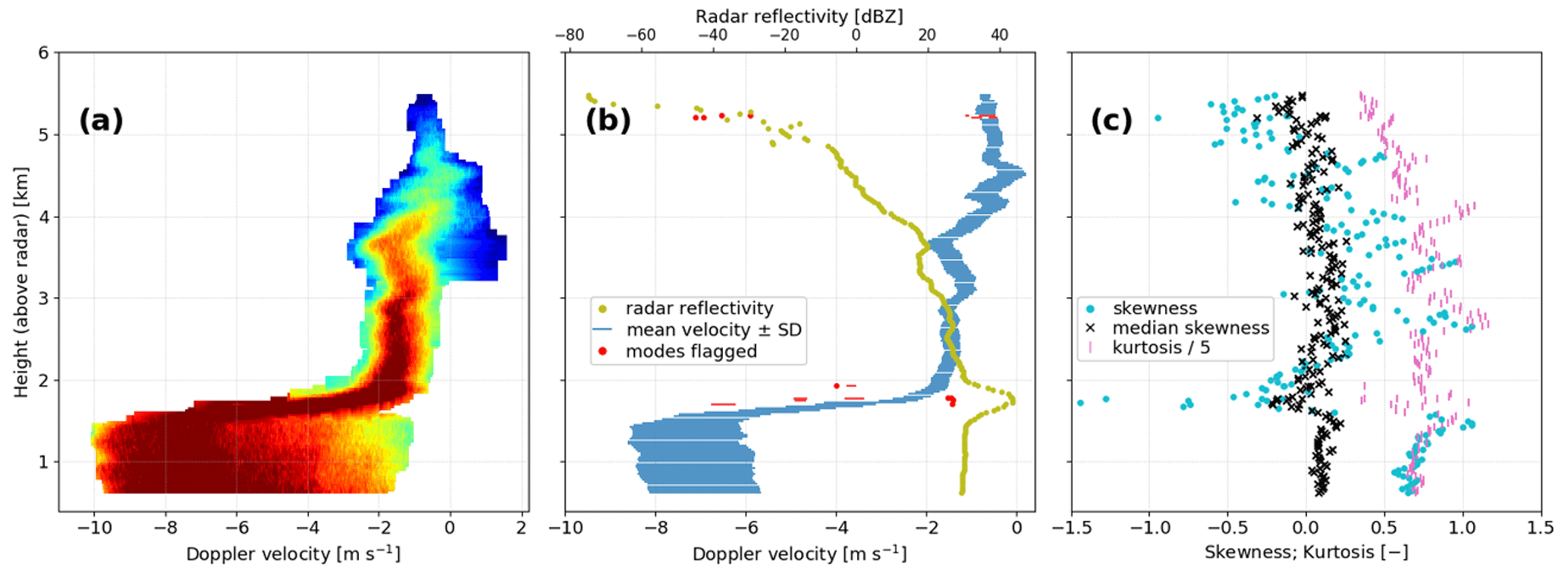
Figure 11 shows a typical stratiform precipitation event. This birdbath scan was recorded at the Essen (ESS) radar in the fall of 2021 at a temperature of 10 ^∘C , comparable to the temperature for the ASB case shown in Fig. 10 (ESS radar lat: 51.405649^∘ N, long: 6.967111^∘ E; alt: 185 m a.s.l.). However, a much higher rain rate of about 3.5 mm h⁻¹ was observed at a precipitation gauge near the ESS radar at the time of the birdbath scan. Figure 11a indicates a lower cloud top height of less than 6 km compared to about 8 km in Fig. 10a and a much stronger precipitation signal. The radar reflectivity above and below the melting layer, which is found at heights between 1.5 and 2 km according to Fig. 11b, is greater than 20 dBZ and thus already higher than the maximum radar reflectivity of the radar bright band in the melting layer found in Fig. 10b. The typical particle fall velocities both above and below the melting layer are also higher here compared to the precipitation event analyzed above. This points to the presence of larger precipitation particles in the stratiform precipitation event that was sampled at the ESS radar compared to the example discussed above for the ASB radar. The more intense rainfall characterized by larger rain drops is also evident from the shift in Doppler velocities toward faster (more negative) typical fall velocities of −7 m s⁻¹ near the ground.

In the example shown in Fig. 11, the melting layer again presents a challenge to the radar postprocessing algorithm and produces several erroneously identified secondary precipitation modes. These are again flagged as misleading artifacts based on their unrealistically low radar reflectivity values, as illustrated in Fig. 11b. Then, both precipitation events summarized in Figs. 10 and 11, where snow above the melting layer transitions to rain below, as well as the snowfall event shown in Fig. 8, are characterized by only a single precipitation mode extending from the atmospheric region where the precipitation is first generated down to the ground.

Another stratiform precipitation event similar to the one shown in Fig. 11 was evaluated in the study presented by Trömel et al. (2021) by comparing the Doppler spectra from an MOHp radar birdbath scan with quasi-vertical profiles of polarimetric variables (Trömel et al., 2014; Ryzhkov et al., 2016) and precipitation particle images obtained by airborne imaging probes within the BLUESKY campaign (Kleine et al., 2018; Voigt et al., 2021). The analysis concludes that the meteorological interpretation of radar signatures from polarimetric weather radar observations benefits from combining these polarimetric radar signatures with vertically pointing Doppler radar measurements, particularly for better distinguishing between aggregation and riming as the dominant precipitation particle growth process. Such benefits of combining slant-viewing polarimetric radar measurements and vertically pointing Doppler radar observations to analyze cloud and precipitation processes have previously been investigated only for higher-frequency cloud research radars (Oue et al., 2018; Kumjian et al., 2020). A comparison of the radar birdbath scan with the airborne in situ observations by Trömel et al. (2021) also shows that the cloud top height indicated by the postprocessed birdbath Doppler spectra is similar to the cloud top height inferred from the in situ measurements (within about 500 m for a cloud top height of 7.9 km above the radar, or 8.9 km a.s.l.). This suggests that DWD's C-band radar Doppler spectra provide a full vertical profile of the precipitating cloud above the radar, with sufficient dynamic range to simultaneously resolve the strong radar echoes of heavy rain and the melting layer in the lower atmosphere close to the radar as well as the much weaker radar signal of frozen precipitation aloft up to the cloud top region.

Figure 12 Summary of analysis results for a birdbath scan recorded in intense frontal rain at DWD's Dresden (DRS) radar in July 2021 (data timestamp: 11 July 2021, 15:59:16 UTC), analogous to Figs. 8, 10, and 11.

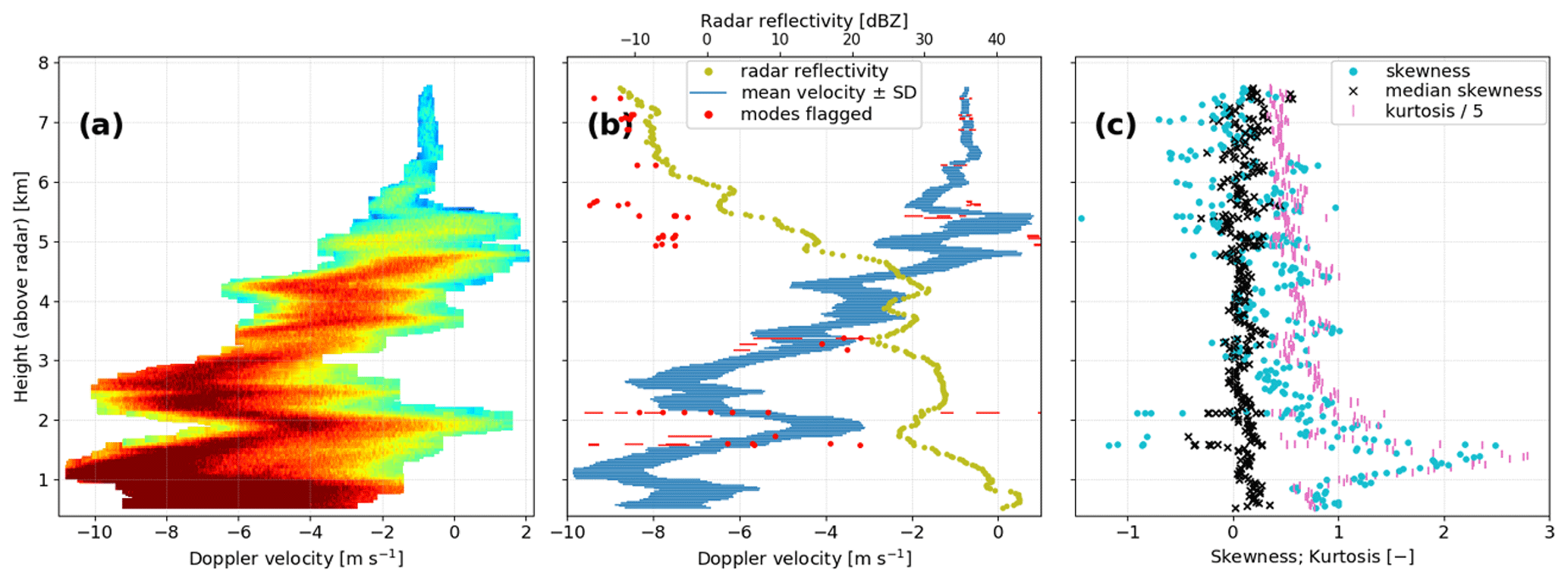
To explore the potential use of DWD's C-band radar birdbath scans beyond the interpretation of snowfall and predominantly stratiform rain events, Fig. 12 summarizes analysis results for a birdbath scan recorded by the Dresden (DRS) radar during an intense frontal shower in the summer of 2021 (DRS radar lat: 51.124639^∘ N, long: 13.768639^∘ E; alt: 263 m a.s.l.). Around the time of the birdbath scan, a strong cold front passed over the radar site. According to a nearby in situ sensor, temperatures plummeted from 25 to 18 ^∘C while the front moved through from the southwest with wind gusts of up to about 15 m s⁻¹, and highly variable rain rates were observed between 10 mm h⁻¹ and potentially as high as 50 mm h⁻¹.

For Doppler spectra recorded in these extreme precipitation conditions, parts of the fully automated postprocessing chain proposed in Sect. 2 break down and have to be replaced by a simpler manual thresholding method. Finding an appropriate threshold for separating the radar signal due to precipitation particles from non-meteorological contributions to the radar output proved to be a delicate task, in particular. In contrast to the previously discussed birdbath scans, small variations in the threshold levels for the two polarimetric parameters that are used to isolate the weather signal according to Sect. 2.2 also have a significant impact on which Doppler velocity bins are still included in the weather signal and on the subsequently calculated quantitative characteristics following Sect. 2.4. While, generally, adequate filter thresholds for the polarimetric parameters between values of 1.0 and 1.6 dB are found by the automated postprocessing algorithm when snowfall and stratiform rain are investigated, e.g., thresholds $\mathrm{C}\mathrm{1},\mathrm{C}\mathrm{2}=\mathrm{1.2}$ dB in Fig. 4, here more stringent thresholds of 0.7 to 0.9 dB have to be prescribed a priori to achieve an acceptable separation of the weather signal from clutter and background noise. This leads to the rejection of some parts of the fringes of the weather signal, i.e., Doppler spectra at lower altitudes are cut off at still relatively high power, and thus the full spectral broadening due to atmospheric turbulence is not captured in the isolated weather signal.

Additionally, the need for extensive interpolation during postprocessing introduces numerous erroneously identified precipitation modes in Fig. 12b, similar to what was already observed for the precipitation events in Figs. 10 and 11 inside the melting layer. Therefore, a systematic analysis of intense convective precipitation or of the melting layer in stratiform precipitation will probably require a modification of the postprocessing algorithm toward a simpler methodology that is more robust under these challenging conditions. Specifically for the analysis of intense convective precipitation, the entire spectral domain in the raw Doppler radar output could be analyzed, instead of first separating the weather signal from clutter and background noise as outlined in Sect. 2.2. The clutter signal can potentially be ignored during postprocessing in these cases, because the clutter signal is usually much weaker than the strong precipitation signal here. Furthermore, it may become necessary to determine a suitable threshold of modal peak prominence by trial and error when identifying the relevant precipitation modes contained in every Doppler spectrum, instead of considering all statistically significant modes that are detected automatically as explained in Sect. 2.3.

Despite the challenges in applying the proposed radar postprocessing method to Doppler data collected in such extreme precipitation conditions, large parts of the processed radar signal in Fig. 12a still lead to calculated quantitative characteristics that can provide the basis for a detailed meteorological interpretation. The typical structure of the weather signal, for example, is strongly affected by vertical air movements, leading to a much more irregular profile of Doppler spectra than for the stratiform precipitation discussed above. The mean Doppler velocity and the width of the precipitation mode follow this characteristic zigzag shape closely in Fig. 12b. Additionally, no radar bright band is present due to much stronger turbulent mixing of precipitation particles from different altitudes, and a very high radar reflectivity maximum of over 40 dBZ is observed in the intense rainfall near the ground. The width of the convective precipitation mode is given by typical standard deviations of $\mathrm{0.8}\le \mathrm{SD}\le \mathrm{1.3}$ m s⁻¹ up to a height of about 5 km above the radar. These SD values fall generally between the widths of the rain mode (below the melting layer) calculated for the two examples shown in Figs. 10b and 11b.

Similar to Fig 11c, the higher-order Doppler moments in Fig. 12c again show their most striking features for Doppler spectra where postprocessing leads to significant interpolation, resulting in non-meteorological artifacts particularly at the high-intensity fringes of the isolated weather signal in Fig. 12a, e.g., at heights around 1.5 km above the radar. As the moments of skewness and kurtosis are very sensitive to how asymmetric and how fat the tails of the underlying distribution are, these artifacts then heavily affect the calculations of the higher-order Doppler moments for the corresponding precipitation modes. Nonetheless, the presented C-band radar birdbath scan strategy and the proposed postprocessing method show good promise for a detailed analysis of a wide range of precipitation conditions.

In contrast to Doppler spectra obtained from cloud radars that are often limited to analyzing non-precipitating clouds or only provide a faithful snapshot of the lower part of precipitating clouds close to the radar where atmospheric attenuation at high radar frequencies can still be neglected, the Doppler data collected by DWD's C-band weather radars are not significantly impacted by attenuation effects. This allows an analysis of the full vertical profile of Doppler spectra recorded for diverse precipitation events from snowfall over stratiform rain, including the melting-layer transition from frozen hydrometeors to raindrops, to intense frontal showers.

4 Conclusions

This study presents the new DWD birdbath scan strategy that was implemented by the German Meteorological Service (Deutscher Wetterdienst, DWD) in the spring of 2021. Since then, the vertically pointing DWD birdbath scans provide high-resolution Doppler spectra for all 17 operational radars of the German C-band radar network with an update rate of 5 min. The Doppler spectra are added to the DWD radar database and can then be exploited to investigate the physical processes that drive different types of precipitation, e.g., rimed snow or stratiform rain.

Additionally, a radar postprocessing algorithm was developed to separate the relevant meteorological radar signal contained in the birdbath Doppler spectra from clutter and background noise based on polarimetric characteristics. After isolating the weather signal, the statistically significant precipitation modes in each Doppler spectrum can be identified and quantified by a multimodal analysis. This analysis also provides uncertainty estimates for all calculated modal and multimodal properties of the precipitation modes. The newly designed postprocessing chain and analysis method emphasize automation and flexibility by combining classical signal processing techniques with an unsupervised data mining approach based on clustering, instead of relying on the more traditional practice of manually choosing fixed thresholds for filtering the radar signal.

Analysis results for five birdbath scans recorded at different radar sites illustrate the capabilities and challenges in evaluating various precipitation events, from snowfall over stratiform rain to intense frontal showers. In the initial convective phase of a snowstorm, two precipitation modes can be identified in the processed Doppler data: one mode of significantly rimed snow, characterized by typical particle fall velocities faster than 1.5 m s⁻¹ and an estimated rime mass fraction of RMF>0.5 in the lowest usable radar bins around 650 m above the ground, and a weaker secondary mode of more pristine snow, characterized by typical particle fall velocities slower than 1.2 m s⁻¹ and a corresponding rime mass fraction of RMF≪0.5. The investigated stratiform precipitation events instead feature only a single precipitation mode extending from the cloud top down to the ground. Doppler spectra recorded during the intense frontal shower, with observed radar reflectivities of up to about 40 dBZ, are also dominated by a single precipitation mode but show a more variable profile of the mean Doppler velocity and a large spectral width up to much higher altitudes than the profiles determined for the stratiform precipitation events.

The automated postprocessing algorithm performs well for snowfall and for stratiform precipitation above and below the melting layer. The actual melting layer, as well as frontal showers that are heavily affected by vertical air motions, exhibit polarimetric radar characteristics similar to static clutter and thus present a considerable challenge to the postprocessing scheme. Even if optimal filter thresholds are determined manually by trial and error instead of trusting the automated thresholding procedure, erroneous precipitation modes are identified occasionally. Furthermore, the higher-order Doppler moments of skewness and kurtosis that are calculated for each precipitation mode may suffer from spurious artifacts within the melting layer or in intense frontal precipitation.

Nonetheless, two findings from the presented analysis are especially encouraging both for improving our fundamental understanding of precipitation processes and for evaluating and complementing DWD's operational services:

1. Estimating the typical degree of riming for individual modes of frozen precipitation allows a high-resolution analysis of the principal particle growth mechanisms in precipitating clouds above the melting layer. Future efforts could also include testing another recently introduced approach for retrieving the rime mass fraction from radar Doppler spectra that is less impacted by vertical air movements than the method employed in this study (Vogl et al., 2022). These riming retrievals can then be combined with scanning polarimetric radar measurements or atmospheric wind and temperature fields derived from atmospheric models to provide a more complete picture of precipitation microphysics and atmospheric thermodynamics (Oue et al., 2018; Trömel et al., 2021). Such an analysis of precipitating clouds could be further extended by also incorporating modern in situ precipitation sensors that reveal the precipitation type near the surface and indicate the typical mass and three-dimensional shape of frozen hydrometeors (e.g., Garrett et al., 2012; Singh et al., 2021). Even deeper insight into the major precipitation processes can be gained by adding multifrequency cloud radar observations to the analysis (e.g., Kneifel et al., 2015; Gergely et al., 2017; Chase et al., 2018) or by complementing the C-band radar measurements with observations from co-located and relatively inexpensive K-band Micro Rain Radars (Maahn and Kollias, 2012; Frech et al., 2017).

2. DWD's C-band radar birdbath scans can be used to collect high-resolution Doppler spectra of intense precipitation, thus offering a unique view into severe weather events at the 17 DWD weather radars installed across Germany. Motivated by first successful tests for disentangling folded Doppler spectra when precipitation fall speeds exceed the Nyquist velocity for DWD birdbath scans of 13.3 m s⁻¹, the initial focus will be on gaining new insights into the structure of strong thunderstorms, which cause significant damage across central Europe and in many places around the world (Zipser et al., 2006; Pucik et al., 2019; Nesbitt et al., 2021). Here, C-band radar Doppler spectra from DWD's operational birdbath scan can be used to probe and analyze in great detail storms that move directly over any DWD radar site. The results from the multimodal analysis of the birdbath scans should then help evaluate the operational techniques that are applied for tracking the thunderstorm and estimating precipitation type and intensity while the storm passes over the radar site. These operational techniques form the basis for issuing DWD weather warnings to the public and rely primarily on scanning polarimetric radar measurements (and short-term predictions derived from atmospheric modeling) at a much coarser vertical resolution. The operational algorithms could then be optimized further based on a comparison of operational outputs and the analysis results of the high-resolution birdbath scans (where coincident storm data are available).

Appendix A: Equations for quantitative characteristics

This section lists the equations for calculating the spectral properties introduced in Sect. 2.4 to quantify the precipitation modes at each height level, as well as one additional multimodal property that is not discussed further in this study. The equations for the higher-order Doppler moments generally follow Williams et al. (2018) but are adapted to our spectral radar output that is given as uncalibrated power. The subscript or superscript “tot” indicates variables integrated over the full spectral range, i.e., over all Doppler velocities; “mode” instead specifies variables integrated only over the Doppler velocity range of an individual precipitation mode as defined in Sect. 2.3. Doppler power in individual spectral bins is denoted as ${\widehat{S}}_H\left(v\right)$, explicitly including the spectral dependence in terms of Doppler velocity v. Additionally, the uppercase index H indicates that the variable is given on a dB scale (in the H polarization channel), while a lowercase h instead marks the corresponding variable expressed in linear units.

Converting radar reflectivity and Doppler power spectra between dB scale and linear units according to

$$Z_H^{\mathrm{tot}}=\mathrm{10}{\log }_{\mathrm{10}}{Z}_h^{\mathrm{tot}}$$

and

$$\begin{array}{}\text{(A1)}& {\widehat{S}}_H\left(v\right)=\mathrm{10}{\log }_{\mathrm{10}}{\widehat{S}}_h\left(v\right),\end{array}$$

the radar reflectivity for individual precipitation modes $Z_H^{\mathrm{mode}}$ (dBZ) can be estimated from the Doppler spectrum ${\widehat{S}}_H\left(v\right)$ and the well calibrated overall radar reflectivity $Z_H^{\mathrm{tot}}$ as

$$Z_h^{\mathrm{mode}}={\displaystyle \frac{\sum _{\mathrm{mode}}{\widehat{S}}_h\left(v\right)}{\sum _{\mathrm{tot}}{\widehat{S}}_h\left(v\right)}}{Z}_h^{\mathrm{tot}}$$

$$\begin{array}{}\text{(A2)}& Z_H^{\mathrm{mode}}=\mathrm{10}{\log }_{\mathrm{10}}{Z}_h^{\mathrm{mode}}.\end{array}$$

For each identified mode, the first- to fourth-order moments are also calculated, i.e.,

•  

  the (power-weighted) mean velocity (m s⁻¹)

  $$\begin{array}{}\text{(A3)}& \stackrel{\mathrm{‾}}{v}={\displaystyle \frac{\sum _{\mathrm{mode}}v{\widehat{S}}_h\left(v\right)}{\sum _{\mathrm{mode}}{\widehat{S}}_h\left(v\right)}},\end{array}$$
•  

  the standard deviation (m s⁻¹)

  $$\begin{array}{}\text{(A4)}& \mathrm{SD}={\left[{\displaystyle \frac{\sum _{\mathrm{mode}}(v-\stackrel{\mathrm{‾}}{v}{)}^{\mathrm{2}}{\widehat{S}}_h(v)}{\sum _{\mathrm{mode}}{\widehat{S}}_h\left(v\right)}}\right]}^{\mathrm{0.5}},\end{array}$$
•  

  the (normalized) skewness (–)

  $$\begin{array}{}\text{(A5)}& \mathrm{SK}=\left({\displaystyle \frac{\mathrm{1}}{{\mathrm{SD}}^{\mathrm{3}}}}\right){\displaystyle \frac{\sum _{\mathrm{mode}}(v-\stackrel{\mathrm{‾}}{v}{)}^{\mathrm{3}}{\widehat{S}}_h(v)}{\sum _{\mathrm{mode}}{\widehat{S}}_h\left(v\right)}},\end{array}$$
•  

  and the (normalized) kurtosis (–)

  $$\begin{array}{}\text{(A6)}& \mathrm{KU}=\left({\displaystyle \frac{\mathrm{1}}{{\mathrm{SD}}^{\mathrm{4}}}}\right){\displaystyle \frac{\sum _{\mathrm{mode}}(v-\stackrel{\mathrm{‾}}{v}{)}^{\mathrm{4}}{\widehat{S}}_h(v)}{\sum _{\mathrm{mode}}{\widehat{S}}_h\left(v\right)}}.\end{array}$$

To complement the moment of skewness defined in Eq. (A5), the median skewness (–), often also called nonparametric skew, can be computed as an intuitive measure of the asymmetry of the precipitation mode, after determining the median velocity v_med (m s⁻¹):

$$\begin{array}{}\text{(A7)}& \mathrm{MES}={\displaystyle \frac{\stackrel{\mathrm{‾}}{v}-v_{\mathrm{med}}}{\mathrm{SD}}}.\end{array}$$

In addition to the modal properties presented in Eqs. (A2) to (A7), several multimodal properties are calculated that quantify the relation among multiple simultaneously occurring precipitation modes when more than a single mode is found in the analyzed Doppler spectrum. Here, three parameters are listed that are based on the definitions given by Zhang et al. (2003), who investigated the bimodality of probability distribution functions of tropospheric water vapor in the tropics.

If the peak Doppler power for every precipitation mode i is expressed as $S_{i,\max }\left(v\right)=max{\widehat{S}}_{i,H}\left(v\right)$, the corresponding multimodal ratio (here, the difference on a dB scale) of the peak power and the maximum of all modal power peaks can be determined as

$$\begin{array}{}\text{(A8)}& {\mathrm{MMR}}_i=S_{i,\max }\left(v\right)-max{S}_{i,\max }\left(v\right).\end{array}$$

MMR then quantifies the strength of each precipitation mode relative to the strongest mode in the Doppler spectrum. Instead of using the peak power S_i,max(v) in the definition of MMR, the integrated power $\sum _{\mathrm{mode}}{\widehat{S}}_{i,H}\left(v\right)$ could be used alternatively.

For two precipitation modes i and j with mean velocities ${\stackrel{\mathrm{‾}}{v}}_i<{\stackrel{\mathrm{‾}}{v}}_j$, the normalized bimodal separation (–) is an estimate of the distance between the centers of the two modes normalized by the widths of the modes:

$$\begin{array}{}\text{(A9)}& {\mathrm{BMS}}_{ij}={\displaystyle \frac{{\stackrel{\mathrm{‾}}{v}}_j-{\stackrel{\mathrm{‾}}{v}}_i}{\mathrm{2}({\mathrm{SD}}_i+{\mathrm{SD}}_j)}}.\end{array}$$

The overlap of two adjacent modes i and j can be quantified through the bimodal amplitude (dB):

$$\begin{array}{}\text{(A10)}& {\mathrm{BMA}}_{ij}=S_{ij,\min }\left(v\right)-S_{i,\max }\left(v\right).\end{array}$$

Here, S_ij,min(v) denotes the trough, or minimum Doppler power, between the two modes and $S_{i,\max }\left(v\right)<S_{j,\max }\left(v\right)$. Then, BMA specifies the prominence of the smaller Doppler peak. The closer BMA is to BMA_max=0, the greater is the overlap of the two mode peaks, indicating stronger mixing of the underlying precipitation processes.