Coincident in situ and triple-frequency radar airborne observations in the Arctic

The dataset collected during the Radar Snow Experiment (RadSnowExp) presents the first-ever airborne triple-frequency radar observations combined with almost perfectly co-located and coincident airborne microphysical measurements from a single platform, the National Research Council Canada (NRC) Convair-580 aircraft. The potential of this dataset is illustrated using data collected from one flight during an Arctic storm, which covers a wide range of snow habits from pristine ice crystals and low-density aggregates to heavily rimed particles with maximum size exceeding 10 mm. Three different flight segments with well-matched in situ and radar measurements were analyzed, giving a total of 49 min of triple-frequency observations. The in situ particle imagery data for this study include high-resolution imagery from the Cloud Particle Imager (CPI) probe, which allows accurate identification of particle types, including rimed crystals and large aggregates, within the dual-frequency ratio (DFR) plane. The airborne triple-frequency radar data are grouped based on the dominant particle compositions and microphysical processes (level of aggregation and riming). The results from this study are consistent with the main findings of previous modeling studies, with specific regions of the DFR plane associated with unique scattering properties of different ice habits, especially in clouds where the radar signal is dominated by large aggregates. Moreover, the analysis shows close relationships between the triple-frequency signatures and cloud microphysical properties (particle characteristic size, bulk density, and level of riming).

1 Introduction

There are currently two spaceborne atmospheric radars in operation: the Global Precipitation Measurement Dual-frequency Precipitation Radar (GPM DPR) and the CloudSat cloud-profiling radar (CPR) whose missions have been foundational for characterizing the evolving nature of clouds and precipitation on Earth over the last decade. The CPR on board CloudSat is a 94 GHz nadir-looking radar (Stephens et al., 2008), unique in its ability to sense condensed cloud particles whilst coincidentally detecting precipitation. While the CPR was not specifically designed for rain retrieval, its data have shown great potential for rain estimation (Haynes et al., 2009) and snowfall estimation in particular, providing vertical profiles of snowfall rate along with snow size distribution parameters and snow water content (Matrosov et al., 2008; Hiley et al., 2011). The joint NASA/JAXA GPM mission (Hou et al., 2014), launched at the end of February 2014, aims at providing global measurements of precipitation with higher accuracy and a wider coverage in latitudinal span (65^∘) than those obtained by the Tropical Rainfall Measuring Mission (TRMM) (Iguchi et al., 2000; Nesbitt and Anders, 2009). The GPM Core Observatory carries a dual-frequency precipitation radar (DPR) system including a Ka-band (35.5 GHz) radar and a Ku-band (13.6 GHz) radar. The GPM DPR detection performance is slightly improved compared to the TRMM precipitation radar (PR), with a minimum detectable signal (MDS) of 14.5 dBZ at Ku and 16.3 dBZ at Ka in the matched scan (MS) mode (Hamada and Takayabu, 2016). The inclusion of a second frequency in GPM has already demonstrated improvement in many aspects such as the ability to retrieve parameters characterizing the drop size distribution (DSD) in rain (Gorgucci and Baldini, 2016) and value in improving the rain classification (Le and Chandrasekar, 2016​​​​​​​). Moreover, coincident measurements from the CloudSat CPR and the GPM DPR of the same precipitating system have illustrated that centimeter and millimeter radars are effective in mapping different parts of the precipitating system and can be used synergistically in order to better retrieve cloud microphysical properties (Battaglia et al., 2020a). Following the guidelines provided by the 2017–2027 Decadal Survey (National Academies of Sciences, Engineering, and Medicine, 2018), multi-frequency Doppler radars, with different combinations of Ku, Ka, and W bands, have been proposed as the core instruments of the Aerosol Cloud Convection and Precipitation (A-CCP) mission GHz) (Kummerow et al., 2020; Battaglia et al., 2020a). Multi-frequency radar observations are especially valuable in ice–snow cloud conditions because of the large variability in scatterers' microphysical properties (e.g., particle size, shape, and density). The use of multiple radar frequencies, at least one of which is in or close to the Rayleigh regime (centimeter wavelength) and one is sufficiently affected by non-Rayleigh scattering (millimeter wavelength), has been proposed to improve retrievals of cloud properties over single-frequency applications (Sect. 2). Better understanding of ice cloud characteristics and composition will relax assumptions made on the retrieval of precipitation rate of ice (von Lerber et al., 2017) and ice water content (IWC), which is needed to understand the global distribution of the ice-phase precipitation, thereby enhancing our knowledge of the global water and energy budget.

Despite the valuable information the existing spaceborne systems have been providing so far, gaps in the detection and characterization of precipitation remain, especially when the capabilities of multi-frequency radar observations of ice and snow are considered (Battaglia et al., 2020a). Triple-frequency measurements have been made using ground-based campaigns (e.g., the 2019 TRIple-frequency and Polarimetric radar Experiment – TRIPEx, Dias Neto et al., 2019; the 2015 Biogenic Aerosols Effects on Clouds and Climate – BAECC – field campaign, Kneifel et al., 2015). The Parameterizing Ice Clouds using Airborne Observations and Triple-frequency Doppler Radar Data (PICASSO) campaign (Westbrook et al., 2018) has also been making ground-based triple-frequency measurements along with coincident in situ aircraft measurements of the microphysics. The co-location is very accurate as the radar dish is steered automatically using the real-time position feed from the aircraft. To date, very few airborne experiments (e.g., the 2003 Wakasa Bay Advanced Microwave Scanning Radiometer Precipitation Validation Campaign, Lobl et al., 2007, and the 2015 Olympic Mountains Experiment – OLYMPEX, Houze et al., 2017) have collected triple-frequency radar observations but only with limited nearly coincident airborne in situ cloud microphysical data. For example, the OLYMPEX provides 2.2 h of in-cloud data with Ku–Ka–W radar data and coincident microphysics (Chase et al., 2018; Tridon et al., 2019). At the time of this writing, there are no publicly available coincident multi-frequency radar and in situ airborne datasets from high-latitude regions where precipitation is dominated by shallow, low-intensity snow or mixed-phase precipitation.

The RadSnowExp (Wolde et al., 2019) is a multi-platform and multi-sensor study organized by the European Space Agency (ESA) and conducted by the National Research Council of Canada (NRC) and Environment and Climate Change Canada (ECCC) to address the pressing need for provision of precipitation measurements both locally and globally. The research flights were conducted in midlatitudes and near the Arctic circle (Iqaluit, NU, Canada, ∼ 63^∘ N​​​​​​​) during the fall of 2018, covering a large geographical region and wide range of microphysical conditions at a temperature range −50 to 5 ^∘C and altitude extending to 7 km (Wolde et al., 2019). The flights focused on sampling precipitation systems wherein large aggregates and rimed particles were present in order to optimize the triple-frequency analyses. Multi-frequency radar observations were carried out by the NRC Airborne W- and X-band (NAWX) radars (Wolde and Pazmany, 2005) and the University of Wyoming's Ka-band Precipitation Radar (KPR) (Haimov et al., 2018). In addition to the radars, the NRC Convair-580 aircraft was equipped with extensive in situ and remote sensing sensors installed in various locations of the aircraft, including on the underwing and wing-tip pylons, various locations of the fuselage, and inside the aircraft cabin (Fig. 2). The dataset collected in flight during the RadSnowExp campaign contains unique features:

• co-located, high-resolution, triple-frequency radar data with nearly coincident in situ measurements;

• data from state-of-the-art in situ sensors covering the whole scale of atmospherically relevant hydrometeor diameters from aerosol size to precipitation size, along with high-resolution imaging probes for single-particle identification;

• complementary measurements of atmospheric state parameters and cloud-phase detection.

In this study, airborne measurements are used to evaluate findings from recent multi-frequency radar modeling studies that relate such radar signatures to ice particles of varying habits, shapes, and sizes in different precipitation systems including intensive snow events in the midlatitude and high-latitude regions.

This paper is structured as follows. Section 2 provides details on theoretical studies of triple frequency and/or multi-frequency. In Sect. 3, airborne data processing and methodology for the airborne triple-frequency analysis are described. In Sect. 4, the experimental evaluation of a triple-frequency study using the RadSnowExp dataset is presented. Finally, conclusions and discussions are given in Sect. 5.

2 Multi-frequency radar ice retrieval potential

Multi-frequency radar observations are especially valuable in ice–snow cloud conditions. The large variability in ice crystal properties such as density, size, and shape makes the interpretation of single-frequency radar observations extremely challenging. The rationale for multi-frequency radar observations is detailed in recent papers (Ori et al., 2020; Battaglia et al., 2020a, b). In this section, we summarize some of the key results.

When comparing measurements of reflectivities from two radars operating at different frequencies f₁ and f₂ (f₁<f₂), it is possible to consider the dual-frequency ratios (DFRs), defined as their difference in logarithmic units (equivalent to their ratio in linear units),

$$\begin{array}{}\text{(1)}& \begin{array}{rl}{\mathrm{DFR}}_{f_{\mathrm{1}}/f_{\mathrm{2}}}\left(r\right)\left(\mathrm{dB}\right)& =Z_{f_{\mathrm{1}}}^m\left(r\right)-Z_{f_{\mathrm{2}}}^m\left(r\right)=\stackrel{\text{non-Rayleigh effect}}{\overbrace{Z_{f_{\mathrm{1}}}^{\mathrm{nr}}\left(r\right)-Z_{f_{\mathrm{2}}}^{\mathrm{nr}}\left(r\right)}}\\ & +\stackrel{\text{attenuation effect}}{\overbrace{\mathrm{2}{\int }_{\mathrm{0}}^r\left(k_{f_{\mathrm{2}}}\left(r\right)-k_{f_{\mathrm{1}}}\left(r\right)\right)\mathrm{d}r}}\end{array},\end{array}$$

where $Z_{f_{\mathrm{1}}}^m\left(r\right)$ and $Z_{f_{\mathrm{2}}}^m\left(r\right)$ are measured radar reflectivity factors (dBZ) at range r and frequencies f₁ and f₂, respectively, and $Z_{f_{\mathrm{1}}}^{\mathrm{nr}}\left(r\right)$ and $Z_{f_{\mathrm{2}}}^{\mathrm{nr}}\left(r\right)$ are reflectivity factors due to non-Rayleigh effects. $k_{f_{\mathrm{1}}}\left(r\right)$ and $k_{f_{\mathrm{1}}}\left(r\right)$ denote specific attenuation (dB km⁻¹) at range r.

In Eq. (1), we have highlighted the two possible contributions to the DFR:

• “non-Rayleigh effects”, i.e., differences in the effective reflectivity factors of the targets which occur when the hydrometeor sizes are comparable to the radar wavelength (Bohren and Huffman, 1998; Lhermitte, 1990);

• “attenuation effects”, i.e., differences in the attenuation properties along the propagation path, with higher attenuation produced at higher frequencies (Lhermitte, 1990; Tridon et al., 2020).

Non-Rayleigh effects result from intensive properties of the particle size distribution (PSD) (e.g., characteristic size, spread of PSD), whereas attenuation effects can be used to infer extensive quantities (e.g., concentrations, rain rates, equivalent water contents). Because of the variety of ice habits and shapes, the computation of scattering properties of ice crystals is much more complex than for raindrops (Kneifel et al., 2020, and references therein); whilst at small sizes backscattering cross sections are proportional to the square of the mass of the crystals (Hogan et al., 2006), when approaching large sizes the mass distribution within the particle along the direction of the impinging radiation plays a key role in affecting the particle scattering properties (Hogan and Westbrook, 2014). An example of DFR calculations for exponentially and gamma-distributed ice crystals is shown in Fig. 1 where data points diverge from the origin, which corresponds to the Rayleigh approximation when the particle size increases. There is clearly large variability in the triple-frequency observables introduced by the different shapes and degree of riming of the ice crystals, as thoroughly demonstrated in Mason et al. (2019).

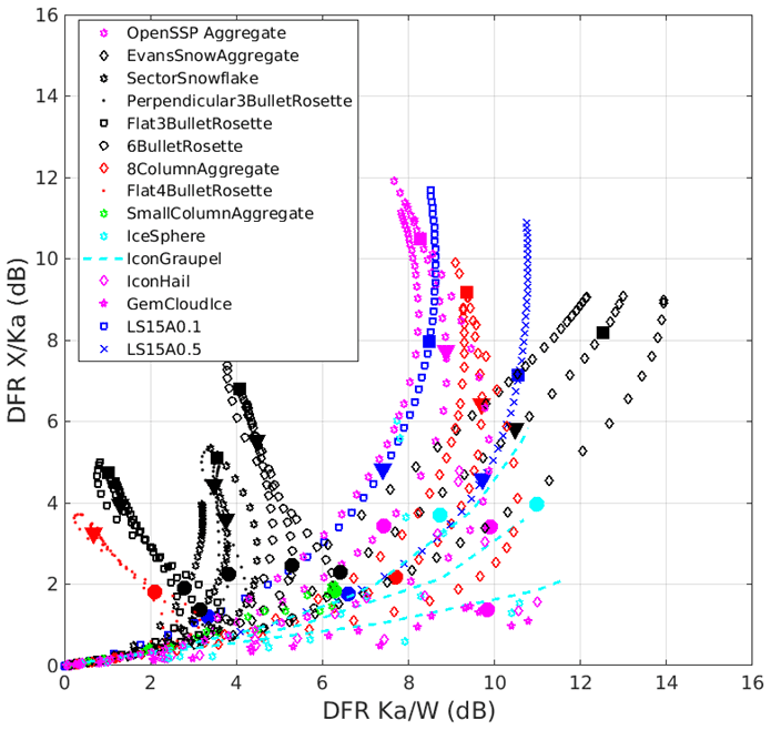
Figure 1 Example of DFR Ka/W vs. DFR X/Ka corresponding to different populations of snow habits with different characteristic diameters of PSD. The habits correspond to state-of-the-art scattering models: the first habit is a mixture of aggregates from the database described in Kuo et al. (2016); the next 14 habits are extracted from the ARTS scattering database (Eriksson et al., 2018); the last three habits are from the models of Leinonen and Szyrmer (2015). For the first two classes of models, scattering properties are computed via discrete dipole approximation for gamma PSD with the shape parameter μ equal −2, 0, and 8 (same symbols); for the last class the self-similar Rayleigh–Gans approximation (for the corresponding coefficients see details in Mróz et al., 2021a​​​​​​​) is used with exponential PSDs. The characteristic mean mass-weighted maximum size of the particle size distribution increases with the curve moving out from the origin (that corresponds to Rayleigh particles with all DFRs being equal to zero). For each line the thick filled circle, triangle, and square markers represent values of D_m equal to 2, 4, and 6 mm, respectively.

3 Data and methodology

3.1 Airborne radars

In this study, triple-frequency radar data from the NRC airborne W- and X-band radar (NAWX) and the Wyoming K-band Precipitation Radar (KPR) measurements from nadir- and zenith-looking antennas are used. The NAWX antennas are housed inside an unpressurized blister radome mounted on the right side of the aircraft fuselage (Fig. 2a), and the KPR radar was installed on the left wing-tip pylon. Some important radar parameters are given in Table 1. More detailed information on the NAWX radar system and KPR can be found in Wolde and Pazmany (2005) and Haimov et al. (2018), respectively. In the RadSnowExp project, the radar complex I and Q samples are processed to powers and complex pulse pair products according to the radar parameter specifications table. Although the three radars are almost co-located, additional signal processing steps are needed to provide the highest level of radar volume matching to reduce the DFR estimation errors and to provide the best evaluation of the radar measurements in synergy with in situ microphysics observations.

Table 1 Radar parameters for the RadSnowExp campaign.

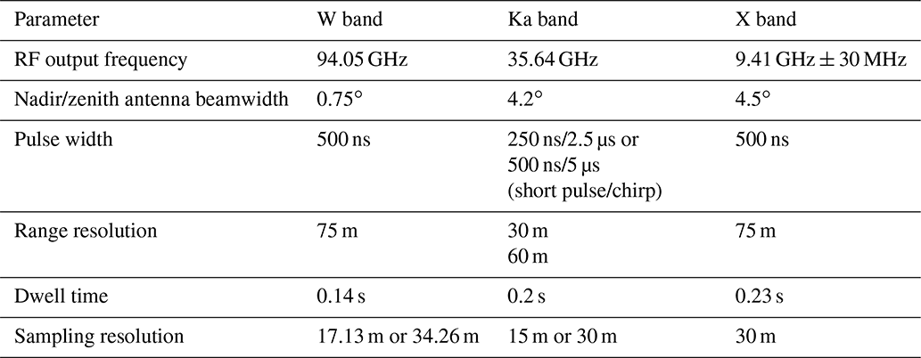
Figure 2 (a) Locations and direction of the NRC airborne W-band (NAW) and X-band (NAX) radars and antenna beams as well as (b) wing-mounted microphysics sensors and air data probes.

3.1.1 Radar data volume matching

To obtain accurate estimates of DFR, radar reflectivity observations at each frequency would optimally sample the exact same volume: that is, the observations would have perfectly matched horizontal and vertical resolutions and would be obtained simultaneously. This is not the case with the RadSnowExp dataset due to mismatched radar beamwidths, vertical resolutions, and radar data dwell times. Hence, additional processing steps are needed to mitigate these mismatches. The 3 dB beamwidths and vertical sampling of the Ka- and X-band radar are 4.2^∘ and 30 m as well as 4.5^∘ and 30 m, respectively, whereas those of the W band are 0.75^∘ and 34.26 m. The volume matching procedure is described in the following steps.

• Re-alignment of data along the range axis. During aircraft rolls, distance from KPR (mounted on the aircraft wing tip) to the radar volume can be slightly different from that of NAWX. Re-aligning radar data along the range axis is required. The re-alignment of the KPR data with the NAWX radar was done by using the ground as a reference point. We observe in most cases that range alignment for KPR is within 30 m.

• Smoothing. This step is performed to reduce the effect of the beamwidth and vertical sampling mismatch. At close range (∼ 245 m) where radar resolution volumes are small, we assume that the condition of uniform beam filling is met. First, a boxcar average filter with a window length of six radar samples is applied to NAW data along the time axis. Resultant NAW data will have an effective beamwidth of 4.5^∘ along the flight path, which is close to that of NAX and KPR radars. Secondly, data from the three radars are mapped onto a common range axis with the origin at the aircraft location and a grid of 35 m, which is close to the vertical sampling of NAW. Next, measurements from the three radars are temporally averaged to 0.5 s. Vertical profiles were recorded every 0.14, 0.23, and 0.2 s for NAW, NAX, and KPR, respectively, and then averaged in post-processing to one profile every 0.5 s. Consequently, co-located triple-frequency radar data are binned into a common grid of 0.5 s × 35 m (time × range​​​​​​​) or 50 m × 35 m at the Convair average ground speed of 100 m s⁻¹. This simple smoothing algorithm mitigates the volume mismatch due to the radar location differences (the NAW and NAX radars are co-located but the KPR is about 10 m away), given the assumption of cloud homogeneity within 50 m along the flight path.

3.1.2 DFR calibration at close range

Calibration for NAWX nadir antennas is made using clear-air observations of the water surface backscatter cross section (Li et al., 2005). Calibration for other NAWX antennas and KPR is done by comparing measurements between antenna ports. More details on calibration and results for NAWX and KPR radars are described in Nguyen et al. (2019). Figure 3 shows an example of radar vertical reflectivity profiles from nadir antennas for a RadSnowExp flight on 22 November 2018. At that sampling time, data from in situ imaging probes (not shown) indicate that the aircraft sampled a region of small ice particles with median volume diameters (MVDs) less than 300 µm, which is in the Rayleigh scattering region of the three radars (see Table A1 in Battaglia et al., 2020a); i.e., the difference between reflectivity factors at Ka band and W band is negligible and between X band and Ka band is about 0.2 dB (Matrosov, 1993). Hence, the differences in the equivalent reflectivities from the three frequencies should mainly depend on the frequency differences of the dielectric factors (${\left|K_w\right|}^{\mathrm{2}}$). However, it can be seen that, at distances close to the radars, there are large mismatches between the measurements (Fig. 3b). This is explained by the limitations of the radar hardware that affect the measurements at this range, within a few first pulse lengths when the receivers reach their steady state. For this study, it is critical to obtain reliable radar data that are as close as possible to the aircraft so that the radar and the in situ sensors sample nearly the same volume. In addition, at close distances, the effect of radar attenuation on the radar reflectivity is minimal. Within a couple of hundred meters, radar attenuation at Ka and X band in snow–ice clouds is negligible. W-band attenuation caused by atmospheric gases, water vapor, and ice scattering in snows–ice clouds would be also minimal at a distance <300 m. Data at the first few range gates in the far-field distance of the radars, collected in regions of small ice particles near cloud tops, were used to compare the W band to the X and Ka band. The W band is used as a reference because of its better sensitivity level, and the first usable range gate (where the data are not affected by close-range biases) is smallest at 245 m. Results show that, at a range of 245 m, the relative offsets between W–X and W–Ka are nearly constant for each flight. When the offset correction is made and the frequency-dependent dielectric properties of the scatterer are taken into account (i.e., a common ${\left|K_w\right|}^{\mathrm{2}}$ is used for all three frequencies), the DFR Ka/W should be 0 dB and the DFR X/Ka ∼ 0.2 dB. This choice is also consistent with the forward modeling approach in Sect. 2. Figure 4 shows the joint distribution of adjusted reflectivities for the two frequency pairs at regions of small ice particles (MVD < 300 µm) for the whole 22 November flight. In general, the biases in the DFR estimates are less than 1 dB, and the standard deviations are estimated to be 0.77 and 0.8 dB for DFR Ka/W and DFR X/Ka, respectively. It is noted that below −5 dBZ, the KPR signal becomes noisy due to the system's low sensitivity, so it is excluded in the analysis.

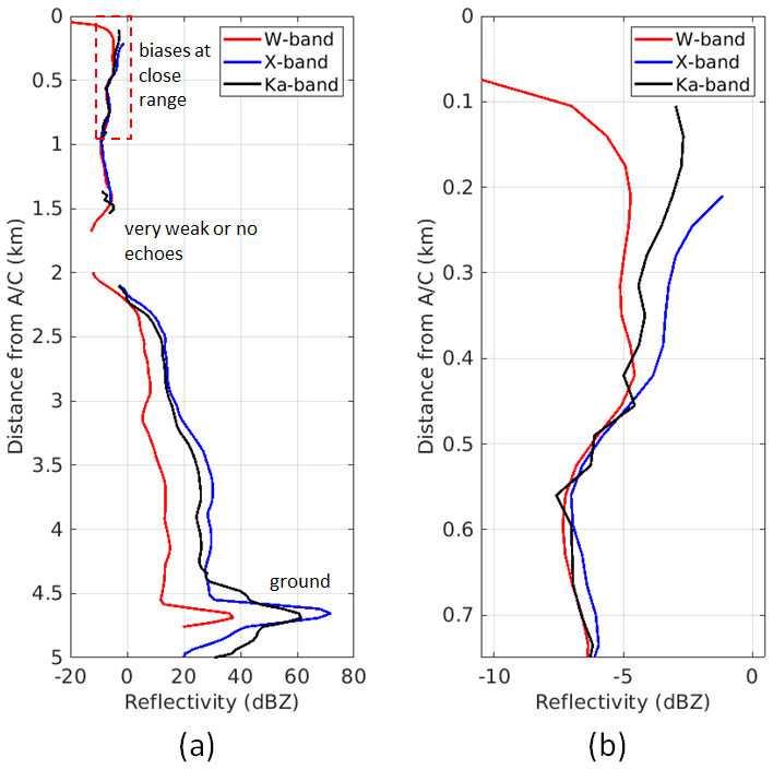
Figure 3 (a) Example of vertical profiles from three radars showing different scattering regimes and (b) close-up plot showing the mismatch of triple-frequency measurements in the close-range region indicated by a box in (a).

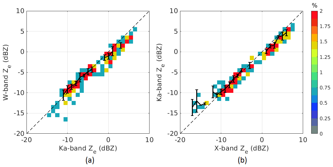
Figure 4 Scatterplots of (a) W-band and Ka-band as well as (b) Ka-band and X-band cross-calibrated reflectivities at 245 m from the nadir antennas for the 22 November​​​​​​​ flight. The data are thresholded by MVD < 300 µm and are binned on a 2D grid with a grid size of 0.5 dB. The dashed black line is the 1:1 line. The solid black lines are the mean curve and 1 standard deviation error bars.

3.2 In situ sensors

For the RadSnowExp project, the NRC Convair-580 aircraft, owned and operated by the NRC, was jointly instrumented by NRC and Environment and Climate Change Canada (ECCC) with state-of-the-art in situ sensors for measurements of aircraft and atmospheric state parameters, as well as cloud microphysical properties. Bulk liquid water content (LWC) and total water content (TWC) were measured simultaneously with particle images and size distribution ranging from small cloud droplets (<10 µm) to large precipitation hydrometeors (>10 mm).

For this work, the cloud particle size distribution was composed using a combination of data from several single-particle probes: fast cloud droplet probe (FCDP, 2–50 µm, SPEC Inc.), two-dimensional stereo (2DS, 10–1200 µm, SPEC Inc.) probe, high-volume precipitation spectrometer version 3 (HVPS3, 150–19 200 µm, SPEC Inc.) probe, and precipitation imaging probe (PIP, 100–6400 µm, DMT). The probes are equipped with anti-shattering tips (Korolev et al., 2013a) and were calibrated with glass beads and a spinning chopper before the campaign and re-evaluated in NRC's altitude icing wind tunnel after the campaign. The uncertainties in sizing and concentrations were less than 5 %. Taking into account image corrections and rejections, the propagated uncertainties can grow within the range presented by Baumgardner et al. (2017). The single-particle data are then used to derive size distributions and bulk cloud properties.

In addition, the Cloud Particle Imager (CPI, 10–2000 µm, SPEC Inc.) provided high-resolution (2.3 µm) grayscale imagery of small cloud and drizzle drops, ice particles and portions of large drops, and ice crystals and broken large ice particles. The high resolution of the CPI probe allows identification of riming levels on ice crystals. In order to aid the determination of triple-frequency radar signatures of various particle compositions and level of riming, the CPI images were classified into 24 different hydrometeor types using machine learning with the convolutional neural network method (similar to Praz et al., 2018) based on a training dataset created from recent projects conducted using the NRC Convair-580. For this paper, we combined some of the classifications and reduced the grouping to nine different types (Table 2). CPI data integrated over 5 s are used to compute and to plot the fractions of sampled particle types. For each study case, we present two CPI particle fraction plots, one for all nine groups listed in Table 2 and one for a subset of ice habits only. The fraction plots are presented in Sect. 4.

Table 2 CPI classification grouping definitions.

TWC and LWC were measured by the Nevzorov, a constant-temperature, hot-wire probe (Korolev et al., 1998). The sensitivity of Nevzorov is estimated to be up to 0.002 g m⁻³ (Abel et al., 2014). We estimate the accuracy of the Nevzorov measurements during RadSnowExp to be on the order of 0.05 g m⁻³, similar to the estimation provided by Faber et al. (2018). Additionally, the Nevzorov water content measurements can be subject to increased uncertainty when large hydrometeors are present (Schwarzenboeck et al., 2009 and Korolev et al., 2013b).

Additionally, the composite PSD, derived from single-particle probes, is used to calculate characteristic sizes (median volume diameter – MVD) and concentrations (N_t). This will minimize the impact of supercooled drops in the calculations and interpretation of parameters characterizing ice particles. The exclusion of small particles does not have a major impact on the calculated bulk microphysics (i.e., bulk density and MVD) and radar reflectivity, which are dominated by large particles. The definitions of several bulk microphysical parameters calculated from the measured PSDs are given below.

• Effective bulk density (ρ_e) is the ratio of the mass of ice to the total volume of ice within a sample volume. An empirical method to compute ρ_e from PSD (Heymsfield et al., 2004; Chase et al., 2018) is defined as

  $$\begin{array}{}\text{(2)}& {\mathit{\rho }}_{\mathrm{e}}={\displaystyle \frac{\mathrm{IWC}}{V}},\end{array}$$

  where IWC is inferred from power dissipated on TWC and LWC sensors of the Nevzorov probe (Korolev et al., 1998) (units: g m⁻³), and V is calculated as the sum of the volume of all particles within the PSD (units: cm³ m⁻³). Thus, ρ_e has units of grams per cubic centimeter (g cm⁻³). Here, each particle is approximated as an oblate spheroid with an aspect ratio of 0.6 (Hogan et al., 2012).

• Median volume diameter (MVD) is defined as the diameter for which the total volume of all drops having greater diameters is just equal to the total volume of all drops having smaller diameters. The in situ derived MVD will be used to evaluate the relationship between the characteristic size of the PSD and the DFRs (Kneifel et al., 2015). MVD can be described as

  $$\begin{array}{}\text{(3)}& {\int }_{D_{\min }}^{\mathrm{MVD}}V\left(D\right)N\left(D\right)\mathrm{d}D={\int }_{\mathrm{MVD}}^{D_{\max }}V\left(D\right)N\left(D\right)\mathrm{d}D,\end{array}$$

  where V(D) is the volume of a particle as a function of size and is calculated in the same way as in the calculation of effective bulk density.

• Particle number concentration (N_t) is calculated as follows.

  $$\begin{array}{}\text{(4)}& N_{\mathrm{t}}={\int }_{D_{\min }}^{D_{\max }}N\left(D\right)\mathrm{d}D\end{array}$$

  Among the three RadSnowExp project flights (22, 25, and 28 November 2018), two were carried out in the Arctic (22 and 25 November) and the third was conducted in midlatitude. The case studies we are looking at are from 22 November 2018, which we chose because larger values of MVD were more frequent than during the other two flights.

3.3 Co-locating radar and in situ measurements

Co-locating radar and in situ measurements is a critical step for accurate determination of relations between microphysics and radar scattering properties. Coincident measurements and perfectly matched volumes would provide the most accurate assessment. However, in reality, radar sampling volumes are much larger than those of cloud probes and both sample volumes are not spatially co-located. In the literature, co-locating radar and in situ data is often achieved by averaging radar data over a large time such as in ground-based observations (Kneifel et al., 2015) or alternatively finding the nearest airborne radar data points to the in situ measurements (Chase et al., 2018). For example, in Chase et al. (2018), radar and in situ data were obtained from two different platforms, and post-processing algorithms assumed that radar volumes within 10 min temporally and 1 km spatially of in situ were considered co-located. Moreover, the in situ observations were assumed to be characteristic of the entire matched radar volume despite the differences in the radar and probe sample volumes.

In our case, the radars and in situ probes are on the same platform and share a common GPS time server, so their data are temporally synchronized. The temporal sampling rate of the post-processed triple-frequency radar data is 0.5 s (Sect. 3.1.1). For particle probes, data are usually integrated over a period of 2–5 s to ensure their good quality; hence, the radar data need to be decimated to match the in situ measurements. On the other hand, there is a difference in sampling location between the radar and in situ. The nearest reliable NAWX and KPR radar data for triple-frequency analysis are 245 m above or below locations where in situ data were measured (Sect. 3.1.2). Although the setup offers much higher accuracy in radar–in situ measurement coincidence compared to previous studies, it still brings in a question of how the radar data should be processed along the range axis to best characterize the microphysics. In order to answer that question, first we need to examine the variability of DFRs in the range dimension. This is done using data from several flight segments during the RadSnowExp campaign.

3.3.1 DFR variability

The DFR variability studied in this section is defined as the fluctuation in DFR values along the radar range axis and will be analyzed by comparing DFRs computed above and below the aircraft. Figure 5 shows examples of scatterplots of DFRs at the first usable distance (245 m) above and below the aircraft for all data points in a RadSnowExp flight on 22 November 2018. In the region of DFRs < 5 dB, the difference of DFRs in the two directions is often within 2–3 dB, but for DFRs between 10 and 15 dB the difference can be as large as 8–10 dB.

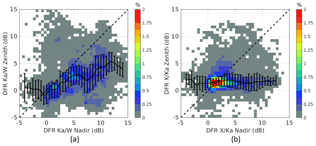
Figure 5 Scatterplots of (a) DFR Ka/W and (b) DFR X/Ka at 245 m above and below the aircraft from the 22 November flight. The data grid is 0.5 dB. The dashed black line is the 1:1 line. The solid black lines are the mean curve and the 1 standard deviation error bars.

3.3.2 Data selection

The DFR variability study in the previous section shows that at a given time, reflectivity ratios between two frequencies could vary up to 8–10 dB within 490 m in altitude, i.e., between the 245 m profiles above and below the aircraft. Averaging radar data over multiple range gates around the in situ sampling might increase biases in DFR estimates; thus, in this study we just use measured DFRs nearest to the in situ sampling. The remaining question is which dataset, above or below the aircraft, should be selected. In order to assess how well the radar data would match the measured particle size distribution (PSD), the equivalent reflectivity factor at X band is forward-modeled from the measured composite PSD using the Rayleigh–Gans spheroidal approximation and Brown and Francis (1995) mass–size relation. The X band is chosen because it is least affected by attenuation and non-Rayleigh scattering effects. The simulated X-band reflectivity is then compared to the NAX radar data using the Pearson correlation coefficient. Correlation coefficients using a 10 min long running window are used to determine flight segments to be analyzed. The 10 min window is chosen to avoid the case in which the cloud field is homogenous (i.e., the correlation would be close to 0) and to reduce the fine variation in the estimated correlations. At the Convair's ground speed of 100 m s⁻¹, a 10 min window corresponds to 60 km. In the environment in which we flew (this Arctic storm), the likelihood of the cloud being homogeneous over a 60 km scale is utterly negligible. On the other hand, if a longer window is used the results will be smoothed out, possibly leading to an inaccurate selection. In this study, data points with correlation coefficients higher than a 0.6 are considered for triple-frequency analysis. Illustrations of this procedure are given in Sect. 4.

4 Triple-frequency case study: Arctic storm on 22 November 2018

On 22 November 2018, the Convair-580 conducted a 3.5 h flight in the Canadian Arctic across the Frobisher Bay area near Iqaluit. Spiral and lawnmower patterns were used for sampling at the outskirts of an Arctic storm, which is clearly visible in the imagery from the AVHRR sensor (channel 4, 10.3 µm) on board the NOAA 13 polar-orbiting meteorological satellite (Fig. 6a). At the beginning of the flight, the aircraft climbed to 6 km and later descended to 1.7 km in steps (Fig. 6b). The next climb was in steps to 2.9 km, followed by descent and landing (Fig. 6b). In terms of cloud properties, mostly mixed-phase conditions were observed, with moderate to heavy icing causing electrostatic discharges on the windshield in the second half of the flight. Diverse hydrometeor habits including rosettes, rosette aggregates, and irregular shapes were sampled during the cruise at an altitude of ∼ 6 km with in-cloud temperature of −40 ^∘C (Fig. 7), whereas pristine plates, capped columns, and densely rimed particles were observed at the lower altitude with temperature centered around −15 ^∘C. Figure 7 shows the ground-to-air temperature and the distribution of the in situ temperature for the 22 November flight.

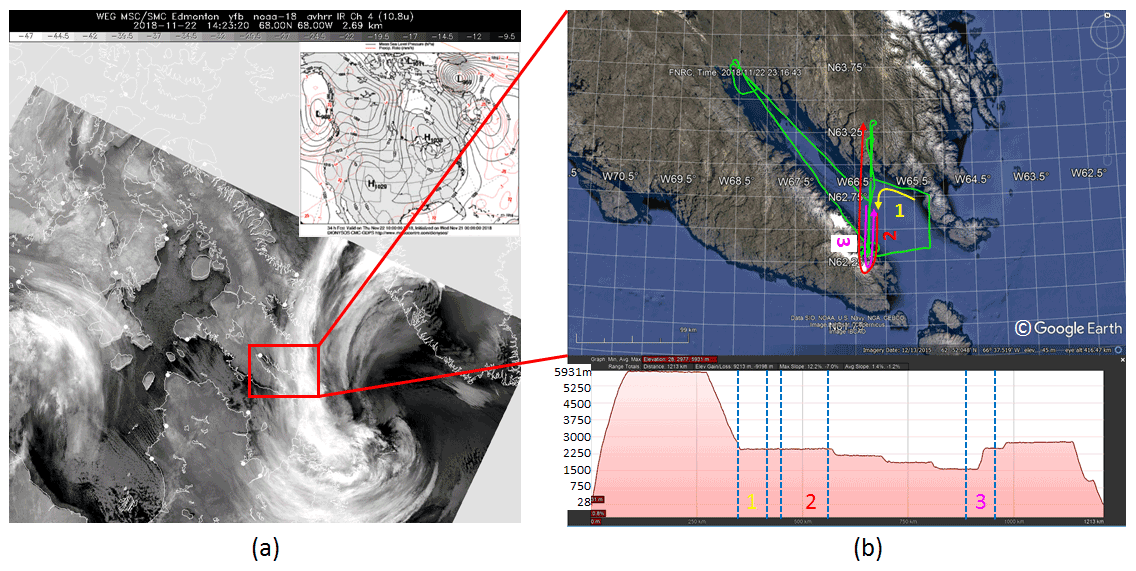
Figure 6 (a) NOAA-13 10.3 µm channel AVHRR imagery showing the Arctic storm. (b) The Convair flight track (green) and altitude plot on 22 November. Locations of three legs used for the case studies in this flight are marked with different colors (yellow, red, and magenta).

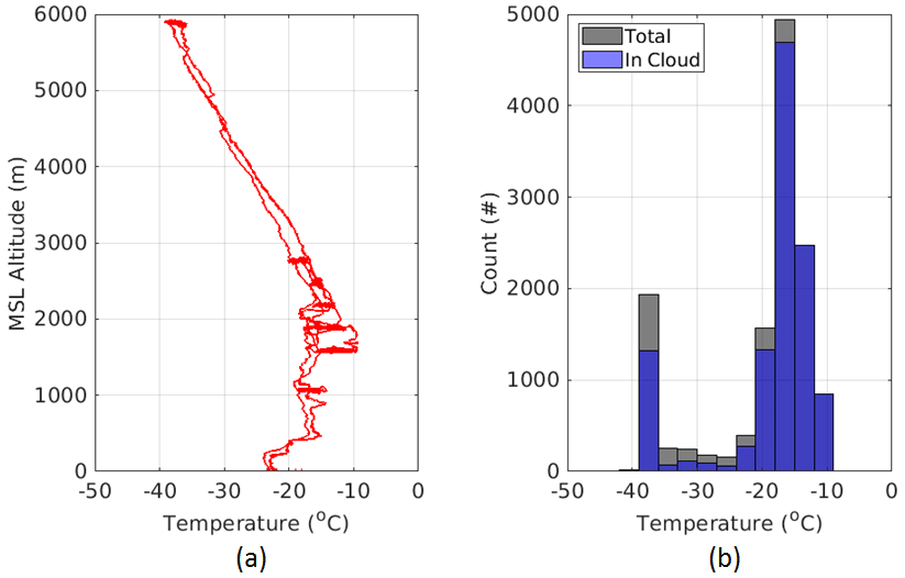
Figure 7 (a) Temperature as a function of altitude for the 22 November flight. (b) Histogram of the in situ temperature shows that for most of the flight the in-cloud temperature was at around −15 ^∘C.

In Fig. 8a, vertical cross section reflectivity at X band of the entire flight is shown. The X-band data are selected to be representative of the radar reflectivity vertical structure of the storm as it is the least affected by attenuation and non-Rayleigh scattering. It is noted that there is a gap in the data at the up antenna of the X-band radar and some residues from the filtering of ground clutter leakages (Nguyen et al., 2022). In addition to the radar time–height reflectivity cross section, radar reflectivity profiles at a distance of 245 m from the aircraft at up and down antennas are depicted along with simulated X-band reflectivity using the in situ PSD data (Fig. 8b). The probability density functions (PDFs) of the X-band reflectivity at the 245 m range above and below the aircraft are shown in Fig. 9. The PDF figures show that the aircraft stayed in inhomogeneous cloud layers (as highlighted by the difference between the nadir and zenith data with higher reflectivities typically occurring below the aircraft). The correlation coefficients between simulated and measured X-band reflectivities (Sect. 3.3.2​​​​​​​) as functions of time are shown in Fig. 8c. For this flight, data from the down antenna often have higher correlation with the in situ data than data recorded at the up antenna. Radar data with correlation coefficients ≥0.6 would be considered to be a good match with the in situ data. In addition to the correlation coefficients, reflectivity values and DFRs are also used to select case studies. In this work, we focus on instances in which non-Rayleigh scattering occurs as indicated by differences in radar reflectivity measured at the three frequencies (Fig. 8d). We have selected three different segments for further analysis of triple frequency (indicated by boxes in Fig. 8), giving a total of 49 min of observations or 588 data points for analysis.

Figure 8 (a) X-band vertical cross section reflectivity for the 22 November flight; (b) reflectivity profiles at 245 m above and below the aircraft along with X-band reflectivities calculated from the measured PSDs; (c) correlation coefficients between the above and below reflectivity and simulated reflectivity; (d) reflectivity profiles of X-, Ka-, and W-band radar at 245 m below the aircraft showing the regions with interesting triple-frequency radar signatures. Boxes indicate the specific segments that will be analyzed further.

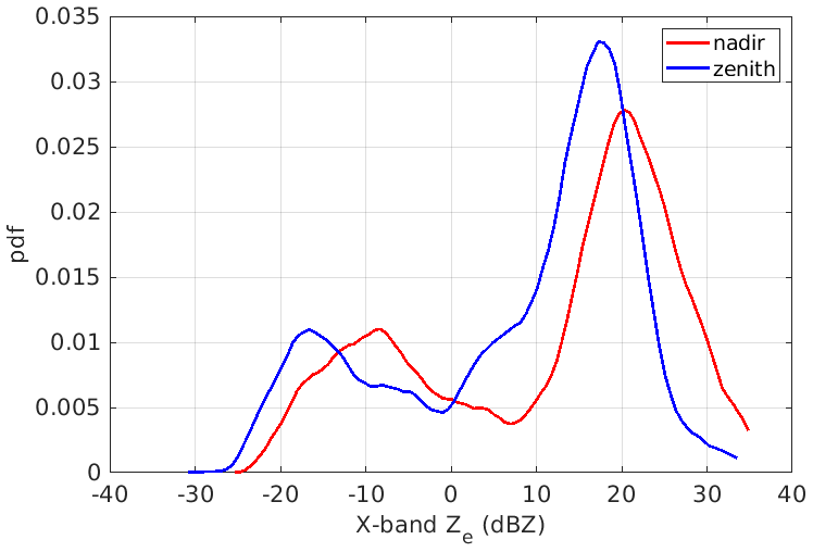
Figure 9 Probability density functions of the X-band reflectivities at 245 m above and below the aircraft for the 22 November flight.

4.1 Segment 1: 19:48–20:00 UTC

In this flight segment, the aircraft descended from 2.8 to 2.4 km with temperatures spanning the range of [−18, −15] ^∘C. During the descent, the aircraft first sampled irregularly shaped ice crystals and small ice in a mixed-phase environment with maximum size <1 mm and then stayed at the same altitude sampling mixed-phase clouds consisting of supercooled cloud drops of various sizes, rimed dendrites, pristine ice crystals, and irregular types. The case is divided into five different sections (A–E) for detailed triple-frequency analysis based on dominant particle compositions that resulted in discernible DFR signatures. In Fig. 10, panels (a)–(e) show time series of the triple-frequency reflectivity, DFRs, PSD spectrum, MVD, ρ_e, TWC, and LWC for this study case. Figure 10f shows the fractional composition of cloud particle types within the CPI detection range (<2 mm) of all major hydrometeor types over time (Table 2), and only the fractional composition of the ice subset is depicted in Fig. 10g. Also, in Fig. 10g, a time series of the differential reflectivity from the side-looking antenna of the X-band radar is shown. The average PSD (Fig. 10h) and mass distribution profiles (Fig. 10i) of the five sections are generally bimodal with two ice modes around 30 µm and 1 mm. In Fig. 10j, representative images of single particles extracted from CPI and HVPS3 for each section are presented.

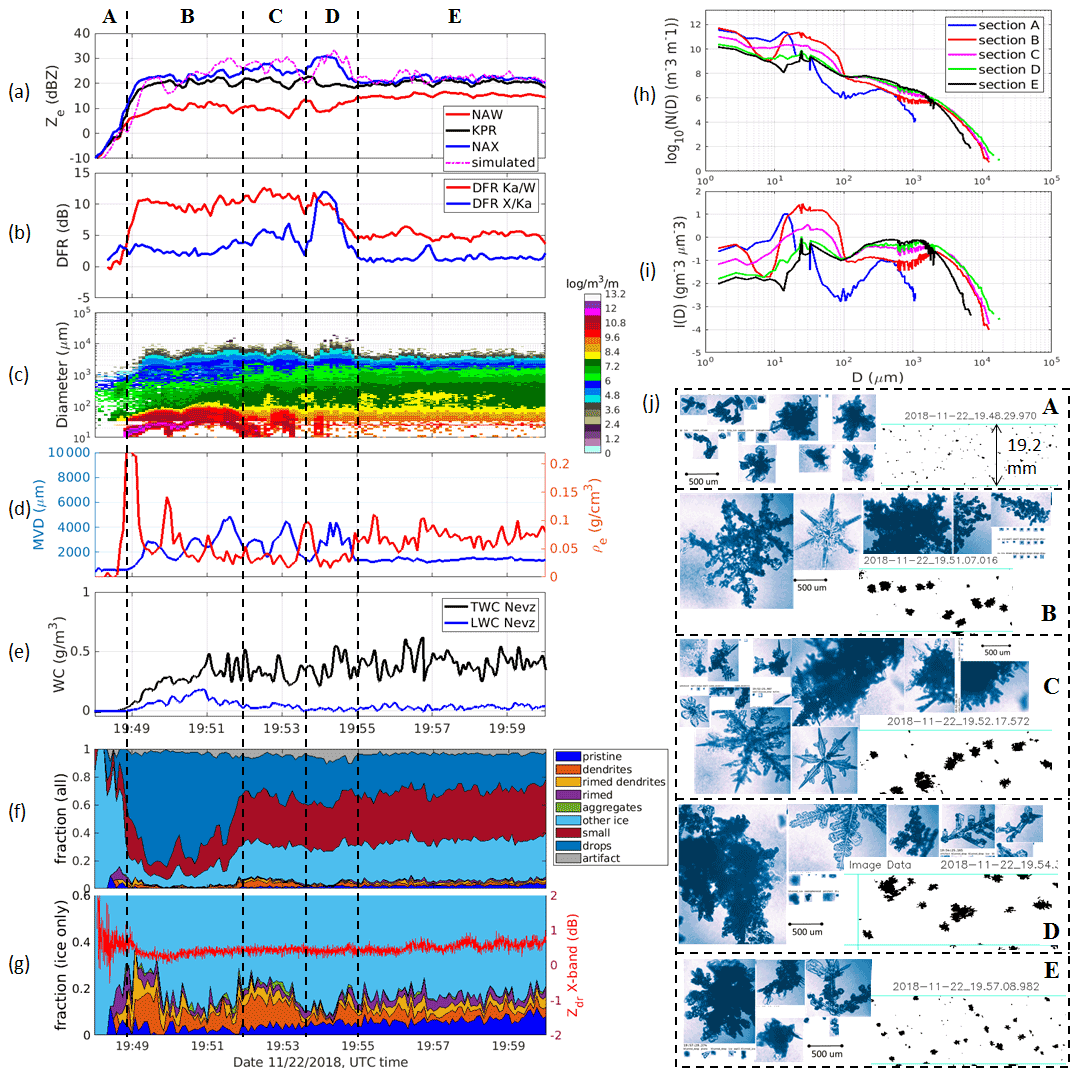
Figure 10 Segment 19:48–20:00 UTC for the 22 November flight: (a) triple-frequency reflectivity profiles; (b) DFR X/Ka and DFR Ka/W; (c) PSD spectrum; (d) characteristic diameters (MVD) and effective bulk density (ρ_e); (e) TWC and LWC from the Nevzorov probe; (f) fractional distribution of all hydrometeors detected with the CPI probes; (e) fractional distribution only of ice habits; (h) averaged PSD profiles; (i) averaged spectral distribution of IWC; and (j) representative images from CPI (blue) and lower-resolution images of large hydrometeors from HVPS3 (black) for each flight section (A, B, C, D, and E). The width of the HVPS3 image strip is 19.2 mm. The BF95 mass–size relationship was used to compute the IWC spectrum.​​​​​​​

In the first section (section A), during descent, the most common habits are irregular and small ice with some densely rimed particles (Fig. 10j). DFR Ka/W is near 0 dB and DFR X/Ka in the [2, 4] dB interval. As the aircraft entered mixed-phase clouds at the start of section B at the altitude of 2.4 km, there was a significant increase in the number of drops and stellar dendrites with some heavily rimed dendritic fragments and graupel. Subsequently, bigger aggregates start to appear in the HVPS3 detection range. At around 19:51 UTC, the fraction of drops (Fig. 10f) increased to its maximum values, which is consistent with the LWC peak (up to 0.2 g m⁻³) observed by the Nevzorov probe (Fig. 10e). With the presence of large particles (dendrites and rimed particles), the DFR values sharply increased to ∼ 10 dB (Ka/W) and ∼ 4 dB (X/Ka). There are some DFR variabilities in this section due to changes in PSD and particle composition. For example, the slight decrease in DFR values around the middle of section B (around 19:50:30 UTC) resembles the decrease in the relative concentrations of dendrites and rimed particles (Fig. 10g). Section C is from sampling of the storm when the aircraft flew in clouds with some heavily rimed dendrites and large aggregates as observed by the HVPS3 probe (Fig. 10j). The fraction of rimed dendrite, unrimed dendrites, and large aggregates increases and the fraction of small drops decreases compared to the second half of section B. It is worth noting that in sections C–E, the percentage of pristine small particles and drop categories is relatively constant. In this section, the DFRs slightly rise, which is consistent with an increase in the proportion of dendritic ice habits (Fig. 10g) with some of them heavily rimed. In section D, heavily rimed, fractured ice and frozen drops are present with bigger aggregates detected by HVPS3 (Fig. 10j). The DFR X/Ka reaches its highest value (∼ 13 dB) exceeding the corresponding DFR Ka/W. Interestingly, this section contains large dendrites with heavy riming and the PSD profile is broader and flatter compared to that of sections B–C (Fig. 10i). It also shows a slight increase in the larger sizes, whilst the fraction of dendrites and rimed particles drops to its lowest level at the first half of the section when the highest DFR X/Ka occurs. Lastly, in section E, an increase in the number of smaller particles in pristine shapes like plates, rimed dendrites, and frozen drops as well as smaller aggregates were detected with the HVPS3. The bulk density is also higher in this section, and the MVD from PSDs are also remarkably stable at about 1.6 mm. The DFR X/Ka and Ka/W are fairly constant around 1.5 and 5 dB, respectively. The reduced DFR values are consistent with a decrease in maximum particle size (Fig. 10h). The small variations in DFR values also agree well with the relatively uniform fraction of cloud particles depicted in the CPI frequency plots (Fig. 10g). In section A, the X-band horizontal Z_dr is noisy due to weak returned signals, but in sections B–D it is clean and remains fairly constant at about 0.5 dB. In section E, Z_dr slightly increases to 0.6–0.8 dB, and this enhancement in Z_dr is consistent with the increase in riming level, which is indicated by the higher bulk density and TWC in this section (Li et al., 2018).

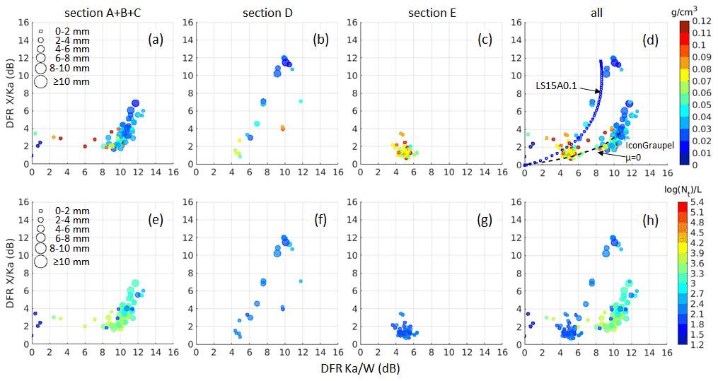
Figure 11 DFR scatterplots for the 19:38–20:00 UTC segment during the November 22 flight. Data points are colored by the effective bulk density (ρ_e) (a–d) and by the total concentration (N_t) (e–h). The dot size is proportional to the calculated MVD. In panel (d), the blue line is for riming model A with an effective liquid water path of 0.1 kg m⁻² (Leinonen and Szyrmer, 2015), and the black line is for a graupel model from Fig. 2.

To characterize ρ_e, MVD, and total concentration (N_t) in the DFR plane, the data are presented in Fig. 11 in such a way that each dot represents a data point, with the size of the dot being proportional to the MVD and the color corresponding to ρ_e or N_t. It can be seen that the DFR values in the five sections (Fig. 10b) populate different zones in the DFR plane associated with unique scattering properties of different ice habits. In general, DFRs increase with increasing coincident MVD, and DFR X/Ka decreases when bulk density increases. There are only few data points in section A (DFR Ka/W ∼ 0 and 2 dB < DFR X/Ka < 4 dB, Fig. 10a) located in regions predicted by modeling of triple-frequency signatures of bullet rosettes (Fig. 1). In sections B and C where the strength of riming increases, the concentration is significantly higher than other regions. The location of data from sections B and C in the triple-frequency plane agrees well with scattering computations of graupel particles using discrete dipole approximation (Fig. 11d). Section D is particularly interesting because of the PSD composition, and only aggregate models (Leinonen and Szyrmer, 2015) are comparable with the observation in the data points (Fig. 11d). The distribution of the data points in this section appears as a nearly vertical curve, which could be attributed to its broader PSD (Mason et al., 2019). In this case, we observed large dendritic aggregates with only a small proportion of rimed cloud particles. Compared to section C, the total concentration of the data points in section D was much lower (Fig. 11e and f), whilst the TWC was larger (Fig. 10e). The data in section E are characterized by higher bulk density values with MVD in the [0, 2] mm interval and are located in a region which overlaps with the modeling results for small aggregates and graupel (Fig. 2).

4.2 Segment 2: 20:05–20:28 UTC

In this case, the aircraft maintained the altitude of 2.4 km but penetrated regions inland from Frobisher Bay (Fig. 6). The segment is divided into three sections (A–C) (Fig. 12) for a detailed analysis. This is still a mixed-phase environment with pockets of high concentration of drops with diameter of approximately 30 µm and an ice mode at ∼ 1.5 mm (Fig. 12i). Different ice habits such as pristine particles, dendrites, fractions of dendritic aggregates, and rimed particles were observed and shown in samples of CPI imagery (Fig. 12j). Larger aggregates (up to 10 mm) were also seen in HVPS3 black shadow images (Fig. 12j). It is worth noting that the particle types observed in the three sections are the same. However, the level of riming and the fraction of dendrites and aggregates within clouds are different between the sections. In section B, the fraction of rimed particles is the highest. The highest TWC (∼ 1 g m⁻³) of the flight was also recorded in section B. During this section, the X-band radar reflectivity increased with a number of high-reflectivity cores at flight level (Fig. 8a), which is consistent with the high TWC (Fig. 12e) and higher relative concentrations of rimed particles and dendrites in the CPI frequency plot (Fig. 12g). In section C, pockets of high TWC were also observed, and the fraction of dendrites and rimed particles remains high with an increase in the relative portion of pristine dendrites and aggregates (Fig. 12g).

Figure 12 Similar to Fig. 10 but for flight segment 20:05–20:28 UTC.

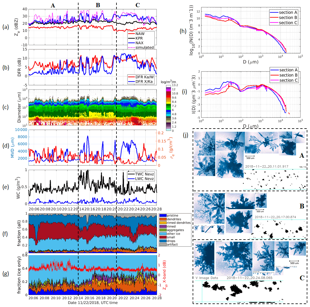
The fluctuation in the time series of the observed DFRs matches that of the cloud particle mean diameters very well (Fig. 12d). It is also consistent with the fraction of rimed particles, dendrites, and aggregates (shown in the CPI composition plot, Fig. 12g). In section A, mean values of DFR X/Ka and DFR Ka/W are ∼ 2 and ∼ 6 dB, respectively, with 1.5 mm < MVD < 4.5 mm, and DFR X/Ka at times reached the same level as DFR Ka/W at around 8 dB when MVD was greater than 4 mm. Also, in section A, side-looking Z_dr fluctuates, at points exceeding 1.5 dB, which we suspect to be a result of dendritic particles and/or needle aggregates dominating the radar measurements. In section B, the DFRs show high variability, resembling the MVD changes, and peaked at ∼ 10 dB for both DFR X/Ka and DFR Ka/W when the TWC was greater than 0.8 g m⁻³ and MVD greater than 6 mm. In region C, the DFR values remain high with the DFR X/Ka reaching over 12 dB. In sections B and C, with the increasing number of large spheroidal compact aggregates due to riming, Z_dr is stable at ∼ 0.5 dB.

Distribution of the data points in this segment in the DFR plane is shown in Fig. 13. Due to large variation in the DFRs, there are overlapping data points between the sections. Section A is characterized by the presence of small particles; hence, it is mainly populated by relatively smaller dots with higher effective bulk density (Fig. 13a). Data points in section B, where the fraction of riming particles reaches its highest value (Fig. 12g), overlap with both sections A and C. Also, in this section, the PSD is flatter and the concentration of small drops is lower (Fig. 12h). In section C, the fractions of dendrites and large aggregates increase, while the fraction of pristine ice crystals drops from the previous two sections. In this case study, the location of all the data points shows a very clear illustration of the “hook signature”, i.e., the DFR Ka/W values decrease, whilst the DFR X/Ka continually increases. Triple-frequency lines for a riming model wherein aggregation and riming are simultaneous in a population of ice crystals (Leinonen and Szyrmer, 2015) are superimposed in the DFR plane. Two scenarios with different levels of riming (e.g., with fixed effective liquid water path of 0.1 and 0.5 kg m⁻²) are shown (Fig. 13d). The modeling results agree with our measurements quite well, although they do not capture the hook signature of the data. This indicates that the amount of riming varied significantly in this flight segment.

Figure 13 Similar to Fig. 11 but for flight segment 20:05–20:28 UTC. In panel (d), the black lines are for riming model A with effective liquid water paths of 0.1 and 0.5 kg m⁻² (Leinonen and Szyrmer, 2015).

4.3 Segment 3: 21:22:30–21:35:00 UTC

For this case the aircraft sampled the precipitation system at a lower altitude of 1.6 km and then climbed up to 2.5 km at the end of the segment (Fig. 6). During this segment there was heavy ice accretion on the aircraft with subsequent electrostatic discharges on the windshield. The X-band Z_dr is stable within [0.4, 0.8] dB, indicating that the radar signals are dominated by spheroidal particles. The segment is divided into four subsections (A–D) based on the DFRs and cloud property signatures (Fig. 19). Section A consisted mainly of supercooled liquid droplets with LWC of ∼ 0.2 g m⁻³ as well as a small fraction of sector plates and heavily rimed (<2 mm) particles (Fig. 14). DFR X/Ka and Ka/W are, in general, around 2 dB, which is consistent with this type of cloud particle. Effective bulk density and concentration are also at their highest values, ∼ 0.8–0.9 g cm⁻³ and ∼10^4.5, respectively. In section B, supercooled liquid droplets and small ice still dominated but started decreasing while millimetric rimed aggregates with MVD ∼ 3 mm appeared. Both DFRs increase when the MVD increases, with DFR Ka/W filling in the entire range from 2–12 dB and DFR X/Ka reaching up to 5 dB. The scatterplot of DFR X/Ka versus DFR Ka/W for these two sections is rather linear and can be characterized by simple spheroid scattering models (Leinonen et al., 2012). In section C, more dendrites and large aggregates with maximum size exceeding 10 mm are found. At the beginning of this section (until 21:27 UTC), DFR Ka/W mirrors the change in MVD. DFR Ka/W goes up to 10–12 dB at MVD ∼ 6 mm, which is similar to the case of section C in the study case 2. However, DFR X/Ka is much lower at 5–7 dB. Moreover, after reaching its highest values (∼ 12 dB), DFR Ka/W starts decreasing, whilst DFR X/Ka continually increases and DFR X/Ka exceeds DFR Ka/W at ∼ 21:27 UTC. Visual analysis of the CPI images reveals the presence of aggregates of rimed dendrites with lower density (Fig. 14j) during this period. Also, the PSD in this section is broader and flatter (Fig. 14i), which affects the distribution in the triple-frequency plane (i.e., the data points are located in an almost vertical line). After 21:27 UTC, DFR Ka/W decreases, whilst DFR X/Ka increases, thus creating a turning point at DFR Ka/W ∼ DFR X/Ka ∼ 8 dB (Fig. 15d). The location of the triple-frequency data in this section overlaps with a region where different snowflake aggregation models exist (Fig. 2). For example, modeling results for an aggregation model described in Kuo et al. (2016) agree reasonably well with the DFR values and patterns in this section.

Figure 14 Similar to Fig. 12 but for segment 21:22:30–21:35 UTC.

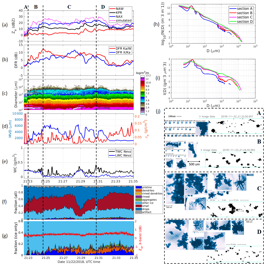
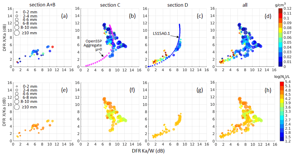
Figure 15 Similar to Fig. 14 but for flight segment 20:05–20:28 UTC. The magenta line (in panel b) is for the aggregation scattering model (Kuo et al., 2016), and the blue line (in panel c) is for riming model A with an effective liquid water path of 0.1 kg m⁻² (Leinonen and Szyrmer, 2015).

In the last section (D), where the aircraft ascended from 1.6 to 2.5 km, the fraction of dendrites, rimed particles, and aggregates with MVD ∼ 1 mm increased at the first half of the section. The bulk density in section D is higher compared to other sections (Fig. 14d), consistent with heavily rimed clouds identified from the CPI probe. Both DFRs start decreasing, similar to a behavior in MVD, and become comparable at around 3–4 dB. The DFR scatterplot for this section, similar to the study case 2, is in great agreement with a riming model described in Leinonen and Szyrmer (2015) (Fig. 15c). Data from all four sections are plotted in Fig. 15d and h, showing a clear hook signature. It is also worth noticing that the concentration in this cloud segment is much higher than in the previous two cases.

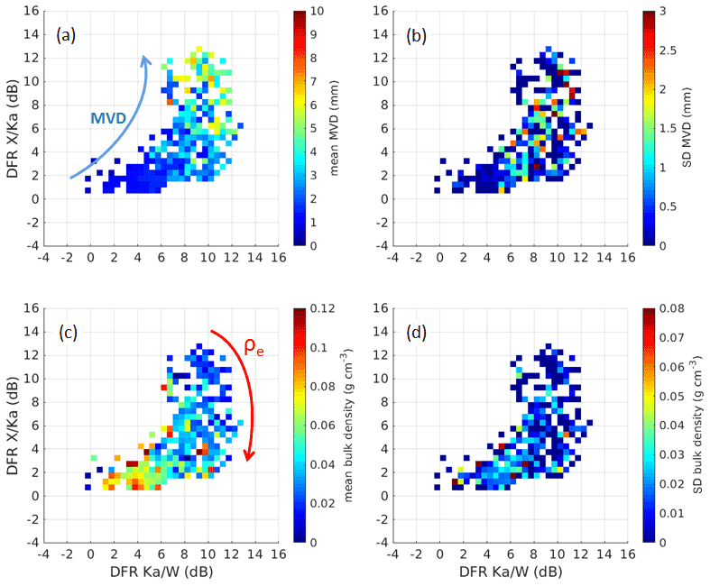
Figure 16 (a) Mean MVD, (b) standard deviation (SD) of MVD, (c) mean ρ_e, and (d) SD of ρ_e calculated from all the data points (573 samples) analyzed in three study cases for the 22 November flight. The data are binned onto a grid with a grid size of 0.5 dB in both axes. The mean and standard deviation are computed from the data within the bin.

Figure 17 Occurrence density plot of (a) Ka-band reflectivity vs. DFR Ka/W and (b) X-band reflectivity vs. DFR X/Ka (b) using nadir data (over 23 500 data points) from the 22 November flight. The black lines present means and error bars (1 standard deviation) of the DFRs.

5 Summary and discussion

The X-, Ka-, and W-band airborne radar observations and almost perfectly co-located in situ microphysical measurements collected during the RadSnowExp project provide an unprecedented dataset for studying multi-frequency radar signatures of snow–ice clouds. The whole RadSnowExp dataset includes more than 12 h of flight data in mixed-phase and glaciated clouds with more than 3.4 h when the scattering was non-Rayleigh for at least one of the radar frequencies. In this study, we careful selected three different flight segments with well-matched airborne in situ and radar measurements of a winter storm in the Arctic region to analyze triple-frequency signatures of various hydrometeor compositions. The dual-frequency ratios (DFRs) in three study cases are observed to be as large as 12 dB, and they appear to be dominated by non-Rayleigh effects. The study cases were observed in a relatively large temperature range between −40 and −10 ^∘C and at different flight altitudes. Efforts were directed toward finding the relationships between ice particle properties and radar triple-frequency observations as well as their potential for developing quantitative retrievals of fundamental ice cloud microphysics. We also provide brief discussions on some measurement aspects (DFR variability and radar sensitivity) which might affect the triple-frequency radar applications.

The results from our study confirm the main findings of previous modeling work with radar DFRs moving within different zones of the DFR plane (Leinonen et al., 2012; Kulie et al., 2014). We find that the size of the crystals has a measurable effect on the triple-frequency signals. The mean particle diameter increases further from the origin of the DFR plane, with increasing DFR values corresponding to increasing MVD. The DFR X/Ka and DFR Ka/W pairs respond to different particle size ranges, with more linear responses for MVD ranges of 2–8 and 1-5 mm, respectively, for the flight we analyzed. However, saturation of DFR Ka/W for large aggregates can produce crossovers between DFR Ka/W and DFR X/Ka. Conversely, the strong connection between the particle size and the triple-frequency radar signature suggests that the data could be directly used to produce lookup tables for mapping measurements in the DFR Ka/W–DFR X/Ka space into microphysical properties like median volume diameter and effective bulk density with associated uncertainties. A first attempt is shown in Fig. 16a–b where all data points from three study cases for the flight on 22 November are used to estimate MVD. In a similar way, effective bulk density of all data points can be averaged and mapped to the DFR plane (Fig. 16c–d). We find that, in general, effective bulk density of ice particles increases as DFR X/Ka decreases and DFR Ka/W increases (ρ_e rotation feature), which in good agreement with findings in other airborne datasets (Chase et al., 2018; Kneifel et al., 2015). These results look promising, but the estimation errors could be high because different combinations of ice particles within the radar volume can produce similar triple-frequency signatures. Future improvement could be obtained by using more data points and a large set of scattering computations; a more quantitative analysis based on a Bayesian retrieval scheme is the topic of a companion study (Mroz et al., 2021b).

With the high-resolution grayscale imagery of cloud particles from the CPI probe, we are able to identify signatures of different types of rimed particles. Regions with DFR Ka/W of [3–12] dB and DFR X/Ka of [2–8] dB are often connected to rimed particles with MVD < 6 mm (although millimeter aggregates could also fit into this region). However, the shape of PSD also has noticeable effects on the distribution of DFR values (Mason et al., 2019). For the same characteristic size, data points with broader and flatter PSD tend to bend away from the horizontal curve (higher DFR X/Ka and lower DFR Ka/W). This feature was demonstrated in section D of segment 1 and in section B of segment 2 where we observed rimed particles with MVD < 6 mm but DFR X/Ka > 8 dB and DFR Ka/W in the range of 6–8 dB. The distribution of rimed particles in the DFR plane found in this study spreads in a much wider region than the findings of Kneifel et al. (2015). On the other hand, large and low-density aggregates occurred in the region with both DFRs greater than 8 dB.

A multi-frequency system is useful because different frequencies are complementary (different sensitivities are exploited) and synergistic (non-Rayleigh scattering effects allow better microphysical retrievals; Battaglia et al., 2020a). If the highest-frequency radar is envisaged to provide sensitivity to small particles (e.g., thoroughly demonstrated by CloudSat) the lower frequencies must cover only the regions where non-Rayleigh effects become tangible. A first clue about where this happens is provided in Fig. 17. In an X–Ka-band (and similarly a Ku–Ka-band) system the lowest frequency ideally should reach at least down to 0 dBZ sensitivity to fully cover non-Rayleigh targets (right panel), with the Ka-band system achieving sensitivities much better than that (thus far better than the current GPM DPR); similarly, in a Ka–W system the Ka-band sensitivity should go down to −5 dBZ (left panel). Recent developments in new technologies make these goals within reach (Battaglia et al., 2020b; Kummerow et al., 2020). Alternatively, an increased DFR dynamic range for small ice particles can be achieved by including observations at frequencies in the G band (Battaglia et al., 2020a; Lamer et al., 2021).

Closure studies that try to reconcile in situ PSD and IWC with remote sensing radar reflectivities remain challenging due to spatial variability of microphysics and mismatch between in situ probe sampled volumes and radar backscattering volumes. Possible solutions can be provided by flight-direction forward- or backward-looking radars or adopting sophisticated phase coding schemes like quadratic phase coding (Mead and Pazmany, 2019) to significantly reduce the blind zone close to the radar or multiple-aircraft coordinated flights.