Three-way calibration checks using ground-based, ship-based, and spaceborne radars

This study uses ship-based weather radar observations collected from research vessel Investigator to evaluate the Australian weather radar network calibration monitoring technique that uses spaceborne radar observations from the NASA Global Precipitation Mission (GPM). Quantitative operational applications such as rainfall and hail nowcasting require a calibration accuracy of ±1 dB for radars of the Australian network covering capital cities. Seven ground-based radars along the western coast of Australia and the ship-based OceanPOL radar are first calibrated independently using GPM radar overpasses over a 3-month period. The calibration difference between the OceanPOL radar (used as a moving reference for the second step of the study) and each of the seven operational radars is then estimated using collocated, gridded, radar observations to quantify the accuracy of the GPM technique. For all seven radars the calibration difference with the ship radar lies within ±0.5 dB, therefore fulfilling the 1 dB requirement. This result validates the concept of using the GPM spaceborne radar observations to calibrate national weather radar networks (provided that the spaceborne radar maintains a high calibration accuracy). The analysis of the day-to-day and hourly variability of calibration differences between the OceanPOL and Darwin (Berrimah) radars also demonstrates that quantitative comparisons of gridded radar observations can accurately track daily and hourly calibration differences between pairs of operational radars with overlapping coverage (daily and hourly standard deviations of ∼ 0.3 and ∼ 1 dB, respectively).

1 Introduction

Operational radar networks play a major role in providing situational awareness and nowcasting in severe weather situations, including heavy rain, flash floods, hailstorms, and wind gusts. Such radar-based information is then used by forecasters as guidance for issuing severe weather warnings. The quality of these radar-derived products in real time is driven to a large extent by how well the underlying radar measurements are calibrated. Recently, the Australian Bureau of Meteorology (BoM) has developed an operational radar calibration framework to monitor the calibration of all BoM operational radars in real time (Louf et al., 2019, hereafter L19). This approach is based on a combination of three techniques. The objective of this technique is to achieve an absolute calibration accuracy better than 1 dB, which is the operational calibration requirement in Australia for quantitative use of the Australian weather radar observations over capital cities (so-called Tier-1 radars). At the heart of this framework lies the so-called volume matching method (VMM), initially developed by Schwaller and Morris (2011) and further improved by Warren et al. (2018, hereafter W18). In this VMM technique, intersections between individual ground-based radar beams and NASA Tropical Rainfall Measurement Mission (TRMM, Simpson et al., 1996) or Global Precipitation Mission (GPM, Hou et al., 2014) scanning Ku-band radar beams are averaged over an optimally defined common sampling volume (see W18 for more detail). In what follows, we will use the term “calibration” to refer to mean reflectivity differences between ground- or ship-based radars and the GPM radar taken as the “reference”. However, it must be noted that reflectivities measured by the GPM radar are not a normed reference, which implies that our use of the term “calibration” is not strictly correct.

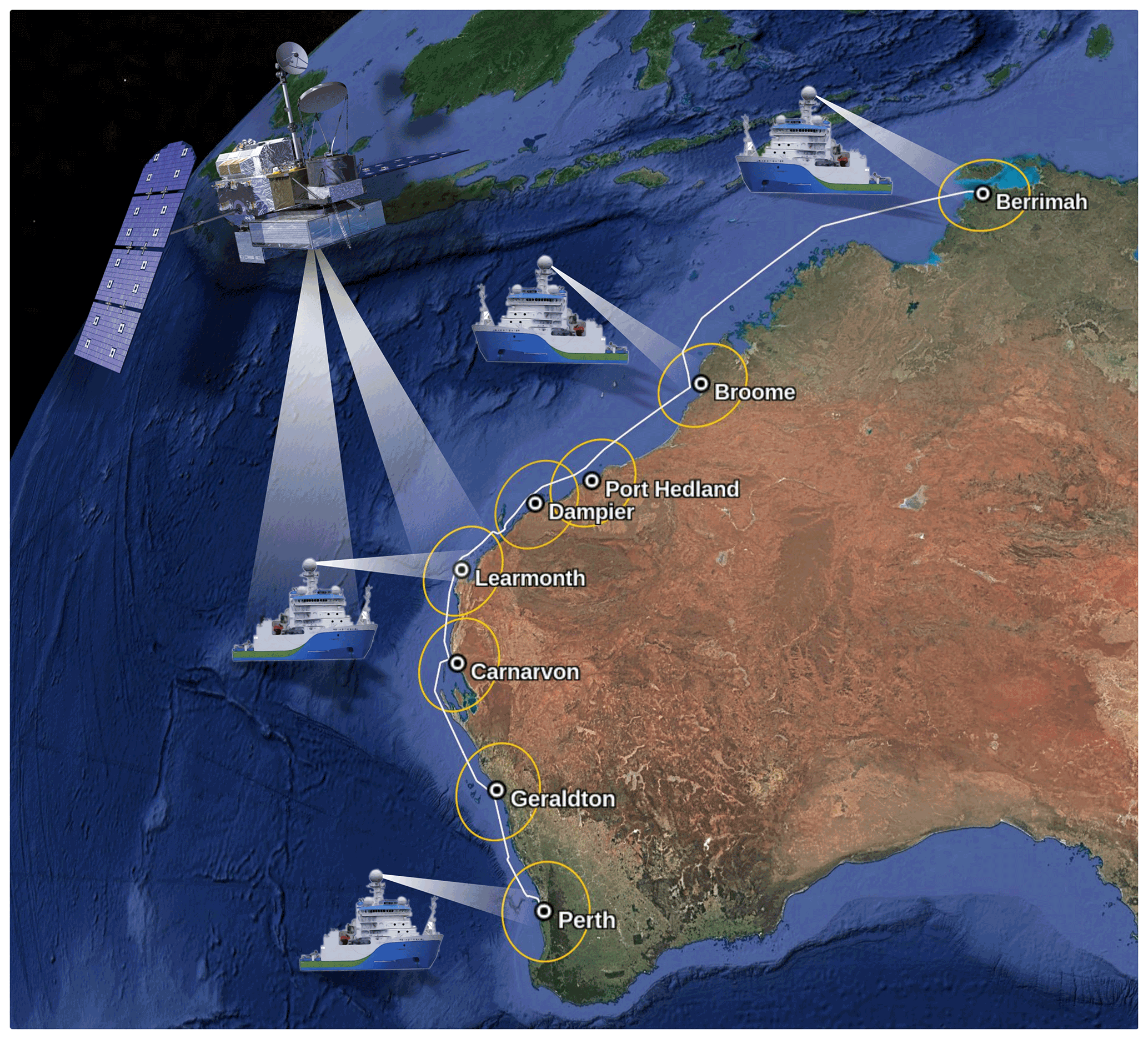
Figure 1 The concept of this study. Ship-based OceanPOL radar and ground-based radars are calibrated independently using the GPM Ku-band spaceborne radar, then all ground radars are compared with OceanPOL during the ORCA voyage as RV Investigator sails south. The 150 km radius of each radar is shown by a yellow circle and the ship track is shown using a white line. © 2021 Google Earth; Map Data: SIO, NOAA, U.S. Navy, NGA, GEBCO; Map Image: Landsat/Copernicus.

A major advantage of using the GPM VMM technique is that the spaceborne radar provides a single source of reference to calibrate all radars of an operational network. This was also well demonstrated by Kollias et al. (2019) in the context of calibrating the U.S. Atmospheric Radiation Measurement (ARM) cloud radar network using the spaceborne CloudSat radar. Despite multiple possible sources of errors contributing to the VMM calibration error estimate, such as temporal mismatch, imperfect attenuation corrections, gridding and range effects, and differences in radar minimum detectable signal, the overall accuracy of such technique is thought to be better than 2 dB for individual overpasses (Schwaller and Morris, 2011; W18; L19). It must be noted, however, that there has been no independent quantification of this accuracy. This was the main objective of this study, where we use dual-polarization C-band weather radar (OceanPOL) observations collected on board the Marine National Facility (MNF) research vessel (RV) Investigator between Darwin and Perth, Australia, as part of the Years of the Maritime Continent – Australia (YMCA, Protat and McRobert, 2020) and the Optimizing Radar Calibration and Attenuation corrections (ORCA) experiments to evaluate the approach of calibrating a whole radar network using GPM. The concept of this study is presented in Fig. 1. GPM observations are first used to calibrate both the ship-based radar and all the operational ground-based radars along the western coast of Australia independently. The ship-based radar observations calibrated using GPM are then individually compared with those from each ground-based radar as the ship sails close to them. Since all radars (including OceanPOL) were calibrated using GPM, the differences between ship-based and ground-based observations can be interpreted as an error estimate of the GPM calibration technique, with some unknown additional contribution from errors due to the ship–ground radar comparisons themselves. These errors coming from ship–ground comparisons are expected to be much lower than those arising from the GPM–ground radar comparisons. Indeed, the advantage of using a ship-based radar relative to a spaceborne radar is that many of the error sources in ground-based–satellite radar comparisons are reduced to a minimum. Taking advantage of a month-long dataset of calibration difference estimates between OceanPOL and the Darwin radar, we also assess the operational potential of daily and calibration change monitoring using overlapping ground-based radar observations.

The remainder of this paper is organized as follows. In Sect. 2, we briefly describe the YMCA and ORCA experiments, the characteristics of radars used in this study, and the calibration techniques. In Sect. 3, we present the main findings of this study. Concluding remarks are presented in Sect. 4.

2 Radar observations during YMCA and ORCA and calibration comparisons

In this section, we briefly introduce the datasets collected during the YMCA and ORCA experiments, the details of all radars involved in this study, and the techniques used to calibrate the ground and ship radars with the spaceborne radar and to compare the ground and ship radars.

2.1 The YMCA and ORCA experiments

RV Investigator OceanPOL radar observations used in this study were collected as part of two back-to-back field experiments. The first experiment is the Australian contribution to the Years of the Maritime Continent (YMCA), which is an international coordinated effort to better understand the organization of coastally induced convection over the Maritime Continent and its complex interactions with large-scale drivers, with the ambition to better represent these processes in global circulation models characterized by large and persistent rainfall biases. During the second phase of YMCA (12 November–19 December 2019), the sampling strategy was to position RV Investigator off the coast around Darwin in a dual-Doppler configuration with either the Warruwi (north-east of Darwin) or Berrimah (Darwin) operational C-band Doppler radars to characterize the rainfall, morphological, and dynamical properties of convective systems developing near the coast and propagating offshore, which are particularly poorly forecasted in this region (e.g., Neale and Slingo, 2002; Nguyen et al., 2017a, b), but are thought to contribute approximately half of the rainfall along tropical coasts (e.g., Bergemann et al., 2015). In this study, we also take advantage of the month-long time series of OceanPOL–Berrimah radar observations to quantify the variability of radar calibration on daily and hourly timescales.

The second field experiment (ORCA) was conducted during a transit voyage to relocate RV Investigator from Darwin to Perth, Western Australia. This transit voyage was an ideal opportunity to collect collocated radar samples with several operational radars along the coast (Fig. 1). Specific stops of 3 h were scheduled in the vicinity of each radar in the event of precipitation within range of OceanPOL and of the ground-based radar. Of the eight possible radars, we were luckily able to collect such collocated precipitation samples for six of them, except Geraldton and Carnarvon. In this study we will use all these collocated samples to quantify how well the calibration estimates provided for each radar by the GPM technique agree with the calibration estimates obtained using OceanPOL as a second and more accurate source of reference.

2.2 The radars of this study

Table 1 summarizes the relevant information about all radars used in this study. The Australian radar network comprises a large variety of radars from different generations, frequencies (although radars in this study are all C-band radars, other parts of the country are covered by S-band radars), beamwidths (ranging from 1.0 to 1.7^∘), range resolutions (ranging from 250 to 1000 m), and total time to complete each volumetric sampling (from 6 min for more recent radars to 10 min for older radars). Several radars of the network are installed in very remote locations, raising specific challenges for the regular maintenance and return to service in the case of hardware failure. As a result, maintaining an accurate calibration of this network is more difficult than in other countries. At the time of the YMCA and ORCA experiments, all radars operated continuously. The Berrimah (Darwin) and Serpentine (Perth) radars are Tier-1 radars (as they cover capital cities), while all other radars in Table 1 are Tier-2 radars. Tier-1 and Tier-2 radars have a calibration accuracy requirement of better than 1 and 2 dB, respectively. The internal calibration accuracy of these operational radars is ideally checked every 6 months by BoM radar engineers as part of their routine maintenance. However, periods between visits can be longer for radars in remote locations. The calibration check only includes measurements of gains and losses at different check points of the transmission and reception chains. No end-to-end calibration using external targets is ever performed. Special visits to sites are organized when a radar is down or when complaints are issued by the public about radar data quality. The extensive recommendations outlined by Chandrasekar et al. (2015) have not been implemented for the Australian radar network yet.

Table 1 Main characteristics of the radars used in this study: radar ID in the operational radar network or platform, name, make, coordinates, frequency band, beamwidth ω (^∘), range bin size Δr (m), and total time to complete the volumetric sampling Δt (min). OceanPOL and all ground-based radars have been manufactured by the Enterprise Electronics Corporation (EEC). n/a – not applicable.

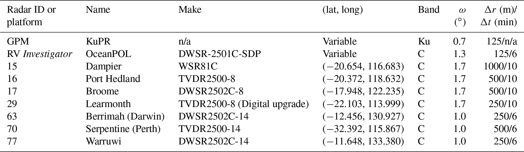
The GPM KuPR and OceanPOL radars are the most modern radars. It must be noted that the OceanPOL radar is the only dual-polarization radar. This important feature for several applications is not used in the present study, except for the quality control of the OceanPOL radar data. A critical aspect of operating a radar on a research vessel is the need to compensate for ship motions and velocity in real time. To do so, the OceanPOL antenna control system ingests the real-time inertial motion unit data from the ship at 10 Hz and steers the radar beam in real time in the requested azimuth and elevation direction. The accuracy of this stabilization has been found to produce a pointing accuracy better than 0.1^∘, even in harsh sea conditions. Doppler measurements are automatically corrected in real time for the Doppler component induced by ship velocity components. Dual-polarization moments are also corrected using the statistical corrections proposed by Thurai et al. (2014). The same calibration procedure as that employed by BoM is used for OceanPOL (internal measurements of gains and losses, no end-to-end calibration), which does not include the calibration recommendations from Chandrasekar et al. (2015).

As discussed previously, the GPM Ku-band radar measurements are considered as the reference for the calibration of all radars in this study. The GPM radar calibration procedure, described in detail by Masaki et al. (2020), is inherited from years of calibration work undertaken as part of the previous satellite radar mission, the Tropical Rainfall Measurement Mission (TRMM). This calibration comprises an internal calibration (monitoring closely the gains and losses of each component of the radar) and an external calibration procedure using a ground-based calibrator and sea surface of well-known backscatter. Importantly, the GPM mission also benefits from extensive field experiments undertaken as part of the ground validation program, including in situ ground and aircraft validation of the products of the GPM mission. By comparing different approaches for the GPM Ku-band radar calibration, Masaki et al. (2020) demonstrated that the accuracy of the radar was well within the ±1 dB requirement. In our study, Version 5 of the GPM 2AKu product was used for all comparisons (Kidd et al., 2017), which includes the latest calibration from Masaki et al. (2020) and contains attenuation-corrected Ku-band reflectivities. GPM attenuation correction is achieved using a hybrid approach combining the traditional Hitschfeld–Bordan technique (Hitschfeld and Bordan, 1954) and the so-called surface reference technique (Meneghini et al., 2004). To compare GPM Ku-band radar with C-band radars in this study, all GPM Ku-band reflectivities were converted to their equivalent C-band reflectivities using Eq. (5) in L19.

2.3 The S³CAR radar calibration framework

Recently, BoM developed the operational S³CAR (Satellite, Sun, Self-consistent, Clutter calibration Approach for Radars) framework to monitor the calibration of the BoM operational radars in real time (operational version of L19). This approach is based on a combination of three techniques. The first technique, the relative calibration adjustment (RCA, e.g., L19; Wolff et al., 2015), assumes that the 95th percentile of “ground clutter” radar reflectivities (buildings, topographic structures, trees, etc. …) within 10 km range is constant. This technique tracks changes in daily calibration to better than 0.2 dB (L19) but does not provide an estimate of the absolute calibration. The second technique (W18) statistically compares collocated ground radar and spaceborne Ku-band radar from the NASA TRMM (1997–2014) and GPM (2014–present) missions. The operational implementation of the GPM calibration technique closely follows the description given in W18. Satellite and ground-based radar observations are first matched to a common volume. We require at least a minimum of 10 satellite profiles within the ground radar domain to select and process a satellite overpass. The melting layer is detected by the operational GPM algorithms and excluded from the matched volumes due to uncertainties in frequency conversions for melting hydrometeors. Matched volumes in both liquid and ice phases are retained (like in W18). Non-uniform beam-filling effects of the matched volumes are mitigated by only selecting volumes that are 95 % filled. A maximum ground-based reflectivity threshold of 36 dBZ is used in the analysis of matched volumes to mitigate the potential impact of attenuation correction errors.

From our experience, and as reported in L19, this technique provides an absolute calibration with an accuracy of approximately 2 dB from each overpass. The S³CAR framework uses the RCA technique to detect stable periods of calibration and averages calibration estimates from all GPM overpasses within each period, improving the absolute calibration accuracy, hopefully to better than 1 dB. Note that these values of 2 and 1 dB are qualitative error estimates based on visual inspection of the variability of calibration error estimates from successive satellite overpasses. The third technique used in S³CAR is the solar calibration technique, which is a faithful implementation of the Altube et al. (2015) method, with additional corrections for a possible leveling error of the radars as described by Curtis et al. (2021). The solar calibration technique uses sun power measurements collected at the Learmonth Observatory, Western Australia. This technique is mostly used in conjunction with the RCA and GPM outputs to diagnose whether a change in calibration is due to the transmitting chain (RCA and GPM detect a change but not the solar calibration technique) or the receiving chain (all techniques detect a change). This is an important diagnostic to help radar engineers troubleshoot a radar issue and enable rapid return to service.

The BoM does not operate a disdrometer network. As a result, the technique outlined by Frech et al. (2017), which compares disdrometer simulations of reflectivity with measured radar reflectivities, cannot be added to the S³CAR framework. In the future, with the increasing number of dual-polarization radars in the Australian network, we are planning to investigate the benefits of the so-called self-consistency of polarimetric variables and may add this technique to the framework.

Among all operational radars considered in this study, only two of these radars (Berrimah and Geraldton) send the unprocessed reflectivities to Head Office in real time, allowing for the full S³CAR process to be used to calibrate these radars. The term “unprocessed” here refers to radar data still containing noise and all typical radar signal contaminations, including ground clutter and sun spikes used in our calibration techniques. For the other radars, post-processing is done on site to reduce the bandwidth required to send the radar data in real time (these radars are in very remote places). As a result, ground clutter and sun interference have largely been removed for these radars, which implies that only the GPM part of the S³CAR framework can be used. As explained, this reduces the accuracy of the calibration estimate for such radars.

2.4 Statistical comparisons between OceanPOL and the ground radars

Calibration between ground-based radars and OceanPOL proceeds by first gridding observations from each radar to a common 1 km horizontal/500 m vertical resolution domain, then building a joint frequency histogram of reflectivity values from all common grid points. The expectation from such plots is that they should exhibit a systematic shift, corresponding to a difference in calibration between the two radars, with a large amount of variability in these comparisons owing to all the sources of errors involved in such comparisons (differences in exact time of observations of a grid, imperfect attenuation corrections, gridding artifacts, differences in implicit resolution of radar volumes at different ranges, differences in minimum detectable signal …). The gridding technique used for all radars is the same and follows Dahl et al. (2019). This gridding technique uses a constant radius of influence (2.5 km) and a weighted summation with distance to the center of the grid for points belonging to the same elevation angle but a linear interpolation along the vertical axis using data from the elevations below and above each grid. This technique has the advantage of not producing the typical artificial vertical spreading of observations below/above the lowest/highest elevation angles observed when using a radius of influence in all directions. Depending on how old the ground radars are, different minimum reflectivity thresholds are used in the comparisons to mitigate potential artifacts in calibration difference estimates due to the degraded sensitivity and reflectivity resolution of the older radars for low-to-intermediate reflectivities. In general, a relatively high threshold of 20–25 dBZ was required, which also had the advantage of reducing the potential impact of different non-uniform grid filling at the edges of the convective systems due to different radar detection capabilities.

OceanPOL data were corrected for attenuation using the Gu et al. (2011) C-band dual-polarization technique available in the Py-ART toolkit (Helmus and Collis, 2016). The operational radars were corrected for attenuation using C-band reflectivity–attenuation relationships derived from the OceanRAIN dataset (Protat et al., 2019). It must be noted that additional comparisons made without attenuation corrections of the ground radars did not yield large differences (less than 0.5 dB in all sensitivity tests conducted). This is presumably due to the fact that there are many more points below 30–35 dBZ than above in those comparisons, resulting in a relatively minor impact of attenuation on these statistical comparisons. Also, the ship and ground radars were generally not far away from each other (typically 20–40 km), and thus the viewing geometry of the storms was quite similar from both radars in most cases, resulting in similar levels of attenuation along the two different paths through the storms.

The scanning sequence employed for OceanPOL uses the exact same 14 elevation angles used throughout the operational radar network. The start of each OceanPOL scanning sequence is synchronized with that of the operational radars running a 6 min sequence (starts on the hour then every 6 min), which implies that temporal differences in volumes sampled by OceanPOL and the radars running the 6 min sequence are minimal. The impact of temporal evolution on the comparisons between OceanPOL and the radars running a 10 min sequence will naturally be larger. To minimize this impact in our comparisons, we have discarded files for which the start time differs from the OceanPOL start time by more than 2 min.

Finally, to mitigate the potential impact of wet radome attenuation at C-band on the comparisons, we screened out observations where precipitation was present within 5 km of either of the radars from the comparisons. More precisely, for each volumetric scan we estimate the precipitation fraction within 5 km, and if more than 20 % of this area is covered with precipitation, we conservatively discard this scan. However, it must be noted that results obtained when changing that threshold were very similar, with maximum statistical differences in estimated calibration difference less than 0.3 dB (not shown). From a visual inspection of radar scans, we inferred that this was due to rainfall generally not observed over and around the radars when such comparisons were made.

3 Results

In this section, we present the main results of this three-way calibration comparison exercise. Comparisons between OceanPOL and the ground-based radars, all calibrated using GPM, are used to quantify the accuracy of the GPM VMM technique. The day-to-day variability of ground–ship radar comparisons over 1 month is also used to quantify the accuracy of daily calibration monitoring using overlapping ground-based radars and its potential for operational use. Lastly, we explore the potential for tracking calibration differences at the hourly timescale rather than the daily timescale using overlapping ground-based radars.

3.1 The accuracy of the GPM VMM technique

As illustrated in Fig. 1, the first part of the calibration consistency check is to calibrate OceanPOL and the ground radars using the same single independent source, the GPM spaceborne radar. All calibration results are summarized in Fig. 2. We are fortunate enough that over 2 months including the YMCA and ORCA observational periods, the rainfall activity allowed us to collect a reasonable number of GPM overpasses over each radar (except for Learmonth, radar 29, Fig. 2). As a result, for radar 29, we will use an older calibration estimate (−2.6 dB), derived from a GPM overpass with many matched volumes in July 2019 and will assume that its calibration has not changed. As discussed previously, the RCA technique can be used to accurately track changes in calibration. Unfortunately, among all radars included in Fig. 2, the RCA can only be applied to radar 63. Additional checks of the outputs of the RCA technique for radar 63 (not shown) indicated that the calibration of radar 63 had not changed over that period, which means that we can simply average all the estimates of calibration error from individual overpasses to come up with a more accurate estimate for this radar 63. Although the RCA technique cannot be used for the other radars, some insights into the calibration stability can be gained from individual calibration estimates from individual GPM overpasses in each panel of Fig. 2. Considering the expected typical error of 2 dB for individual GPM overpasses as a guideline, it seems reasonable to assume that the calibration of the OceanPOL, Warruwi (77), Dampier (15), Broome (17), and Serpentine (70) radars has not changed over the observational period either, with fluctuations around the mean calibration error estimate of less than ∼ 1.5 dB. Results using the solar calibration technique for OceanPOL also indicate that the OceanPOL receiver calibration has remained constant, to within 1 dB, over the study period (sun power of approximately −93 dBm). The Port Hedland (16) radar is more problematic, as the time series shows calibration error estimates ranging from −8 to −2.5 dB over that period. However, the three overpass points closest to the date when collocated observations with OceanPOL were collected (26 December 2019) seem to agree reasonably well (around the mean value of −5 dB); therefore, we will use this value of −5 dB in the following but will keep in mind the lower confidence in this calibration figure.

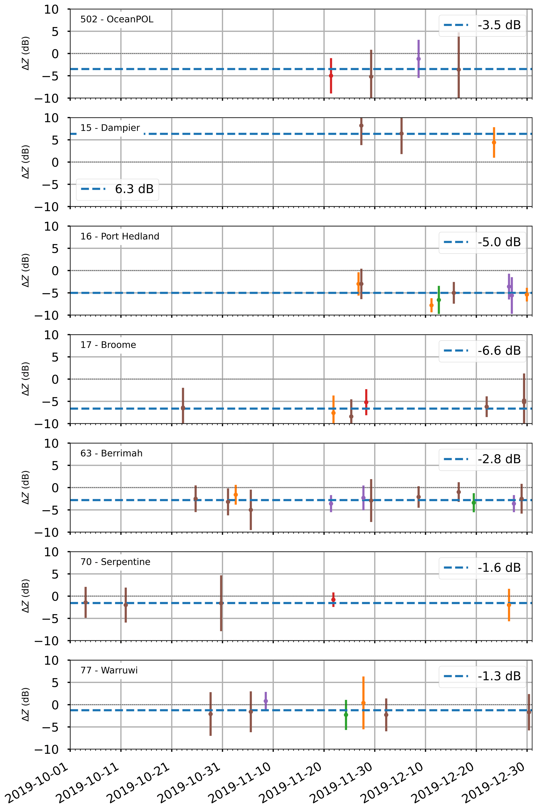
Figure 2 Individual calibration error estimates from the GPM comparisons, for all radars used in this study. The standard deviation of the PDF of reflectivity difference is also shown for each estimate as an error bar. The mean value over the whole period is displayed as a dashed line for each radar, and the value is reported on the upper-right of each panel. Note that a negative value means that the radar is under-calibrated (radar – GPM). The color of each overpass point is the number of matched volumes: fewer than 20 (blue), 20 to 60 (orange), 60 to 100 (green), 100 to 150 (red), 150 to 200 (purple), or more than 250 (brown).

The final step of this calibration consistency check study consists in using the OceanPOL radar (previously calibrated using GPM, Fig. 2) as a second moving reference to compare with the ground-based radars. As explained earlier, satellite–ground comparisons are characterized by multiple sources of errors, including differences in sampled volumes (although great care is taken to match sampling volumes as accurately as possible, e.g., Schwaller and Morris, 2011; W18; L19), non-uniform beam-filling effects, temporal mismatch between observations, differences in minimum detectable signal, and radar frequency differences requiring conversion (most problematic in the melting layer and ice phase of convective storms where this correction is more uncertain, see W18). In comparison, ship radar–ground radar comparisons, especially when radars are, as in this study, reasonably close to each other to minimize differences in sampling volumes, are less prone to all these errors. The radar frequency is the same. The sampling volume and temporal mismatches are also expected to be less problematic (but not entirely negligible, especially for the radars running a 10 min sequence, see discussion in Sect. 2.4). These more accurate ship–ground radar comparisons should therefore be considered as an indirect evaluation of the GPM validation technique and if successful, a demonstration of the value of using such GPM data as a single source of reference for the calibration of a whole national network as is done in Australia with S³CAR.

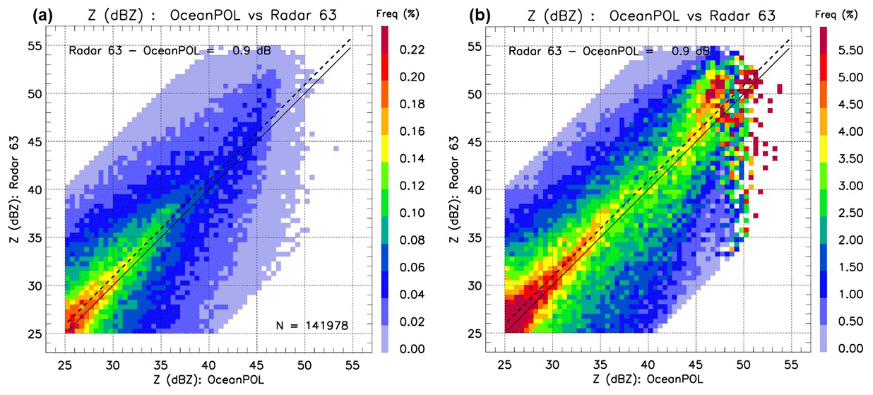
Figure 3 Illustration of 2D joint frequency histograms of reflectivity used to compare quantitatively the OceanPOL radar (x axis) and any of the ground-based radars (y axis), here for the Berrimah radar (63) for 1 day (21 November 2019) of the YMCA experiment. For each plot, the 1 : 1 line is drawn as a solid line, and the calibration difference estimate is written and shown as a dashed line. The colors show the frequency of points falling in each reflectivity pixel 0.5 dB in resolution of the 2D joint histograms, either expressed as the % of the total number of points (a) or as a % of the sum of points for each value of OceanPOL reflectivity (i.e., sum of all points along the y axis at each constant value of the x axis). The number of samples N for this case is 141 978 (see panel a).

Figure 3 shows an example of the 2D frequency histograms of reflectivity that are used to estimate calibration differences between OceanPOL and any of the radars. This particular figure is for the Berrimah radar (63) for 1 day (21 November 2019) of the YMCA experiment. Such frequency distribution plots can be normalized in two different ways. If the number of points in each reflectivity pixel is divided by the total number of points (as in Fig. 3a), it highlights where most of the comparison points are in the reflectivity–reflectivity space, and therefore what contributes most to the mean calibration difference estimate. When the number of points in each pixel is divided by the total number of points in each reflectivity bin on the x axis (Fig. 3b), the joint distribution provides a better visual sanity check of the systematic shift of the joint distribution produced by the calibration difference over the whole reflectivity range and enables detection of other potential artifacts. In the example of Fig. 3a, which is typical of all comparisons made in this study, it is clear that reflectivities less than 35 dBZ contributed most to the estimation of the mean calibration difference of 0.9 dB between the two radars. On the other hand, Fig. 3b shows more clearly that there is indeed a consistent shift in reflectivity values across the whole reflectivity range, as expected from a (systematic) calibration difference. An important feature of Fig. 3 is the large variability observed around the mean calibration difference. The standard deviation of calibration difference for all comparisons in this study was typically between 4 and 6 dB. It must be noted that this large standard deviation is an estimation of the errors on calibration difference of each individual pixel, not that of the daily estimate. The higher number of days spent collecting collocated observations off the Berrimah (63) and Warruwi (77) radars also offers an opportunity to estimate daily calibration differences and take a closer look at the day-to-day variability of calibration differences.

Table 2 Ground radar–OceanPOL calibration difference estimates for all comparisons of this study. A mean calibration difference for radars 63 and 77 that includes all dates and time spans is also provided. For radars 15, 16, and 29, two estimates are provided, with no test on minimum height (AP) or with a minimum height of 2 km for the comparisons (noAP), in an attempt to remove residual anomalous propagation artifacts observed for these radars.

When including all days of observations for radars 63 and 77 (25 d for radar 63 and 4 d for radar 77 with precipitation), the mean calibration difference between OceanPOL and radars 63 and 77 is 0.4 and −0.3 dB, respectively (see Fig. 4 for radar 63, Fig. 5a for radar 77, see also Table 2 for a summary of all calibration differences found in this study). The other relatively recent, better-quality operational radar included in this study is radar 70 (Perth). For this radar, only short-duration drizzle and scattered showers were observed when RV Investigator approached its destination (Fremantle Port), resulting in fewer points for the calibration difference estimate. Despite the short duration dataset for radar 70, the 2D joint histogram of reflectivities shows a consistent difference across the whole reflectivity range, with a mean calibration difference of −0.4 dB (Fig. 5f). These three estimates are well below the required accuracy of 1 dB for operational applications, which indicates that for these four good-quality radars (OceanPOL and radars 63, 77, and 70), the GPM comparisons provided a consistent calibration to within ±0.5 dB. However, those are the comparisons where errors were expected to be smallest, given the large number of days included in the comparisons for radars 63, and the excellent synchronization of the 6 min scanning sequences with OceanPOL for these three radars.

Figure 4 Time series of calibration differences between OceanPOL and radar 63 (Berrimah) during the YMCA experiment. Each colored point is a daily estimate of calibration difference. The color of the point is the number of points for each comparison, and the colored error bar is the standard deviation of hourly calibration difference estimates for that day (see text and Fig. 6 for more details). The solid blue line is the mean value obtained from all these daily estimates (0.4 dB). The overall mean and standard deviation of the daily calibration difference over the period of observations are also included on the lower-right side of the figure. The black dashed line is the zero line. The black points are the daily outputs of the RCA values, with the mean RCA value over the period subtracted and the mean value of calibration difference added, so that the time series is centered on the mean calibration difference value.

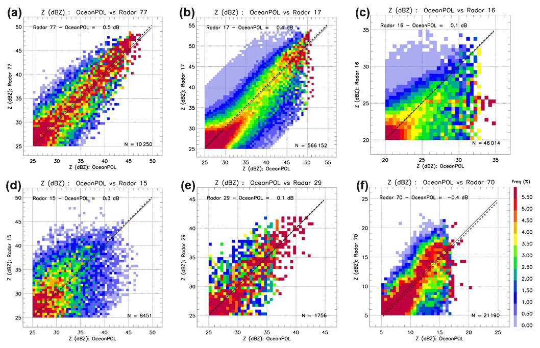
Figure 5 2D joint histograms of reflectivity as in Fig. 3b but for radars (a) 77, (b) 17, (c) 16, (d) 15, (e) 29, and (f) 70. Values of calibration differences are also reported in Table 2. The number of samples N is also given in each panel.

Let us now turn our attention to the quantitative comparisons between OceanPOL and the older operational radars (15, 16, 17, 29) running with a 10 min scanning sequence and/or a degraded range resolution (as reported in Table 1), and only a few opportunistic hours of collocated samples with precipitation (see list of time spans in Table 2). Visual inspection of gridded radar data revealed the presence of strong anomalous propagation (AP) signal in the lower levels (up to approximately 2 km height a.s.l.) for radars 15, 16, and 29, which has not been filtered correctly by the operational radar post-processing suite. This problem is well known to the BoM forecasters. As a result, for these radars, two sets of results are presented in Table 2. Calibration differences obtained from all data are labeled “AP” and those obtained when screening out all common grids below 2 km height are labeled “noAP”. Figure 5 shows the 2D joint histograms of reflectivity when the anomalous propagation is screened out. The largest impact of anomalous propagation is found for radar 16, with a difference of 0.9 dB between estimates with and without AP screening. For the two other radars 15 and 29, the impact is modest (0.3 to 0.5 dB). This is due to the higher proportion of samples located below 2 km height for the radar 16 case (not shown) than for the two other cases. Overall, this result is shown to illustrate that particular attention needs to be paid in regions prone to anomalous propagation effects. From Table 2 and Fig. 5, the calibration differences with OceanPOL for these older radars are +0.3 dB (radar 15), +0.1 dB (radar 16), +0.4 dB (Broome, radar 17), and +0.1 dB (radar 29). In summary, all seven radars considered in these comparisons are characterized by calibration differences with OceanPOL within ±0.5 dB, despite the large variability in radar quality and number of samples included in the calibration difference estimates (reported in Fig. 5). As a result, we can safely conclude that these comparisons validate the concept of using the GPM VMM calibration technique as a single source of reference to accurately calibrate and monitor calibration of national radar networks.

3.2 The accuracy of daily calibration monitoring from overlapping ground-based radars

As introduced earlier, the day-to-day variability of calibration differences between ship- and ground-based radars can be analyzed using the month of collocated samples between OceanPOL and the Berrimah radar collected during YMCA (colored points in Fig. 4). From Fig. 4, some simple statistics can be derived and discussed. The minimum and maximum calibration differences over the month-long time series are −0.2 and +1.1 dB, which corresponds to minimum and maximum differences of −0.6 and +0.7 dB around the mean value of 0.4 dB. The color of the points is the number of samples that were available to estimate the daily calibration difference. The colored error bars are estimates of the hourly standard deviation of calibration difference for each day. From a close inspection of the location of points with respect to the mean value for the period, there does not seem to be any obvious relationship between the number of points and how close the estimates are to the mean value of 0.4 dB. This result shows that the number of samples is not the main source of differences between daily estimates.

The standard deviation of daily calibration difference between Berrimah and OceanPOL over this month of data is 0.33 dB (Fig. 4). Since this standard deviation value includes any potential natural variability of the daily calibration difference and the variability due to uncertainties in these daily ship–ground radar comparisons such as spatial resolution differences and temporal mismatches, this value of 0.33 dB can be considered an upper bound for the uncertainty in daily calibration difference estimates. To check whether the natural variability of daily radar calibration was minimal over that month of Darwin observations, we have added in Fig. 4 the time series of daily mean RCA values (black points) used as part of our operational S³CAR calibration monitoring technique as another calibration variability metric. It has been shown that this RCA technique could track changes in daily calibration to better than approximately 0.2 dB (L19). To better compare variabilities obtained from calibration differences and the RCA, we have subtracted the mean RCA (54.11 dBZ) value from each daily RCA value and added the mean calibration difference over the whole period (0.4 dB), so that the daily RCA time series is centered on the mean calibration difference (blue line). Over this whole period, the standard deviation of the RCA value is 0.12 dB, which confirms the L19 results. This standard deviation is smaller than that of the OceanPOL–Berrimah comparisons (0.33 dB). If we assume that the standard deviation of the RCA value is an upper bound for the natural variability of the daily calibration figure, this result shows that most of the variability in calibration difference between the OceanPOL and Berrimah radars (0.33 dB) is in fact a measure of the inherent uncertainties of gridded radar comparisons. This important result highlights that such quantitative comparisons of overlapping gridded radar observations can be successfully used to monitor the consistency of daily calibration of operational radars with overlapping coverage to better than the 1 dB requirement.

3.3 The accuracy of hourly calibration monitoring from overlapping ground-based radars

The last thing we explore with this Darwin dataset is the potential for tracking calibration differences at the hourly timescale rather than the daily timescale. To do so, for each day of observations, we estimated the calibration difference from 1 h chunks of collocated data, then estimated the standard deviation of the hourly estimates for each day. An example of such daily analysis is shown in Fig. 6 for 1 day (8 December 2019) where 15 successive hours of collocated samples were available. Although this example includes more hours of comparisons than most other days, it is very typical in terms of the hour-to-hour variability we observe each day, making it a good candidate for illustrative purposes. We have not elected to screen out hours with fewer points, which, as can be seen from hours 14 and 15, would have resulted in a lower hourly standard deviation for that case. This should probably be done in an operational implementation. In this respect, the standard deviation of hourly calibration difference presented in Fig. 4 can be considered an upper bound for the hourly standard deviation. The hourly standard deviation is shown in Fig. 6 as a red error bar on top of the daily average point, and as a colored error bar over each daily average in Fig. 4. Over the 1-month study period, the average hourly standard deviation derived from all hourly estimates is 0.8 dB, which is within the 1 dB requirement, but the two extreme values are 0.5 and 1.5 dB (Fig. 4), indicating that occasionally the hourly estimates of calibration difference would not fully meet this requirement. From Fig. 4, it also appears that there is no inverse relationship between the number of samples and the hourly standard deviation, which could have perhaps been expected. For instance, the two points with highest hourly standard deviation (2 and 6 December 2019) are at both ends of the number of samples spectrum, and the three points with the lowest hourly standard deviations are in the lower half of the number of samples spectrum. Figure 4 also shows that when using the hourly standard deviation as an error bar, the mean value over that period (0.4 dB) is always included within 1 standard deviation of the daily estimate. These results would obviously need to be confirmed with more observations in the future but they highlight the potential for hourly tracking of calibration differences, enabling very early detection of issues with operational radars.

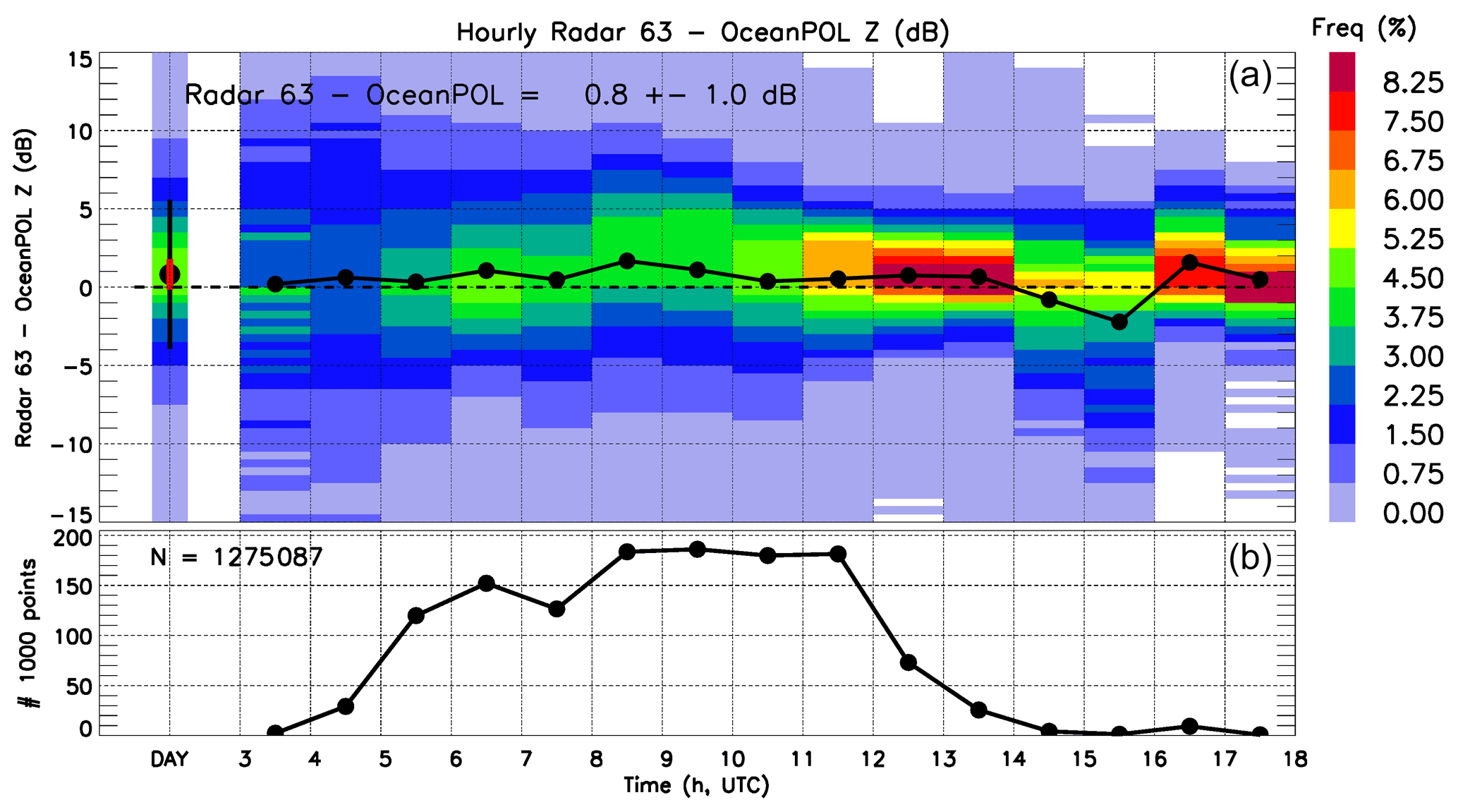
Figure 6 Hourly analysis of calibration differences between Berrimah (radar 63) and OceanPOL for a selected day (8 December 2019). Panel (a) shows each hourly calibration estimate as a black dot, as well as the full frequency distribution of differences within each hour (colors). The first column of panel (a) shows the daily summary, including the mean value (black dot, value is also written), the frequency distribution of calibration differences (colors), the standard deviation of the difference using the N collocated samples (black error bar), and the standard deviation of the hourly estimates of calibration differences for that day (red error bar, value is also written). Panel (b) shows the number of samples in each hour (note y axis is the number of points divided by 1000) and the total number of samples N is also provided.

4 Conclusions

In this study, we used collocated observations between spaceborne, ship-based, and ground-based radars collected during the YMCA (off Darwin) and ORCA (transit voyage between Darwin and Perth) experiments to gain further insights into the suitability and accuracy of using spaceborne radar observations from the GPM satellite mission to calibrate national operational radar networks, and to assess the potential of using data from overlapping ground-based radars to track calibration changes operationally at the daily and hourly timescales.

A major advantage of the GPM VMM technique is that all radars of the network are calibrated against a single source of reference. The GPM VMM literature (Schwaller and Morris, 2011; W18; L19) suggests that errors are of approximately 2 dB from individual GPM overpasses to better than 1 dB when stable periods of calibration can be estimated using the RCA technique and individual GPM estimates can be averaged. However, these errors have never been fully quantified. Using collocated weather radar observations between the OceanPOL radar on RV Investigator and seven operational radars off the northern and western coasts of Australia (all calibrated using GPM), we found that for all seven operational radars, the calibration difference with OceanPOL was within ±0.5 dB, well within the 1 dB requirement for quantitative radar applications (−0.3, +0.4, +0.4, +0.1, +0.3, +0.1, and −0.4 dB). This important result validates the concept of using the GPM spaceborne radar observations to calibrate national weather radar networks.

From the longer YMCA dataset collected when RV Investigator was stationed off the coast of Darwin for approximately 1 month, the day-to-day variability of calibration differences between the OceanPOL and Darwin (Berrimah) radars was estimated and compared with the daily calibration variability estimated using the RCA technique. From these comparisons, we found that the natural variability of daily radar calibration was small over our month of observations (∼ 0.1 dB daily standard deviation). These comparisons also demonstrated that the intercomparison of gridded radar observations had the potential to estimate calibration differences between radars with overlapping coverage to within approximately 0.3 dB at the daily timescale and approximately 1 dB at the hourly timescale. Such technique will be added to our operational S³CAR calibration monitoring framework as an additional calibration monitoring reference between GPM overpasses when the RCA technique cannot be applied.