Calculating the vertical column density of O₄ during daytime from surface values of pressure, temperature, and relative humidity

We present a formalism that relates the vertical column density (VCD) of the oxygen collision complex O₂–O₂ (denoted as O₄ below) to surface (2 m) values of temperature and pressure, based on physical laws. In addition, we propose an empirical modification which also accounts for surface relative humidity (RH). This allows for simple and quick calculation of the O₄ VCD without the need for constructing full vertical profiles. The parameterization reproduces the true O₄ VCD, as derived from vertically integrated profiles, within $-\mathrm{0.7}\pm \mathrm{1.2}\mathit{\%}$ (mean ± SD) for Weather Research and Forecasting (WRF) simulations around Germany, 0.2±1.8 % for global reanalysis data (ERA5), and $-\mathrm{0.3}\pm \mathrm{1.4}\mathit{\%}$ for Global Climate Observing System (GCOS) Reference Upper-Air Network (GRUAN) radiosonde measurements around the world. When applied to measured surface values, uncertainties of 1 K, 1 hPa, and 16 % for temperature, pressure, and RH correspond to relative uncertainties of the O₄ VCD of 0.3 %, 0.2 %, and 1 %, respectively. The proposed parameterization thus provides a simple and accurate formula for the calculation of the O₄ VCD which is expected to be useful in particular for MAX-DOAS applications.

1 Introduction

In the atmosphere, two oxygen molecules can build collision pairs and dimers, which are often denoted as O₄ (Greenblatt et al., 1990; Thalman and Volkamer, 2013, and references therein). O₄ has absorption bands in the UV–visible spectral range; thus O₄ can be retrieved from atmospheric absorption spectra, e.g., by applying differential optical absorption spectroscopy (DOAS) (Platt and Stutz, 2008). Measurements of the O₄ absorption pattern in scattered light provide information about light path distributions in the atmosphere, for instance allowing the investigation of light path length increase within clouds (Wagner et al., 1998) or the retrieval of cloud heights from satellite measurements (Acarreta et al., 2004; Veefkind et al., 2016).

For multi-axis (MAX) DOAS, i.e., ground-based instruments measuring scattered light at different elevation angles, O₄ measurements provide information on vertical profiles of aerosol extinction (Heckel et al., 2005). Prerequisite for MAX-DOAS profile inversions is knowledge about the O₄ vertical column density (VCD) which provides the link between the measured slant column densities (SCDs) at different viewing angles and the forward modeled SCDs based on radiative transfer calculations. Thus, a wrong input of the O₄ VCD directly affects the resulting aerosol profiles. For the profile inversion algorithm MAPA (Beirle et al., 2019) applied to measurements taken during the CINDI-2 campaign (Kreher et al., 2020), for instance, a change of the input O₄ VCD of 2 %, 3 %, 5 %, or 10 % causes changes of the resulting median aerosol optical depth of 6 %, 8 %, 13 %, or 20 %, respectively. Thus, for MAX-DOAS profile inversions, the O₄ VCD should be determined with accuracy and precision better than about 3 %, which limits the impact on resulting aerosol optical depths (AODs) to below 10 % and leaves other sources of uncertainty, i.e., the spectral analysis (≈5 %) as well as radiative transfer modeling (≈4 %) (see Wagner et al., 2021; Table 3 therein) as the limiting factors.

The O₄ VCD can be calculated by vertical integration of the O₂ number density profile squared. This requires knowledge of vertical profiles of temperature, pressure, and humidity, e.g., as derived from radiosonde measurements or meteorological models. However, radiosonde measurements are only available for few stations and do not provide continuous temporal coverage, while modeled profiles might not be available in some cases (e.g., during measurement campaigns in remote regions and poor internet connection; for these cases, profiles from a climatology might be used as fallback option), or they might not reflect the conditions at the measurement site appropriately, in particular in mountainous terrain not resolved by the model.

Measurements of surface air (at 2 m) temperature, pressure, and humidity, on the other hand, are routinely performed by meteorological stations and could be added to any MAX-DOAS measurement site with relatively low costs and efforts. Wagner et al. (2019) proposed to construct full temperature and pressure profiles from the respective surface values by assuming (a) a constant lapse rate of −6.5 K km⁻¹ from ground up to 12 km, and constant temperature above, and (b) applying the barometric formula.¹ Wagner et al. (2019) estimate the uncertainty of the calculated O₄ VCD to 3 % and list the diurnal variation of the surface temperature and the limited representativeness of the surface temperature for the temperature profile above the boundary layer as the main source of uncertainty.

The method proposed by Wagner et al. (2019) reproduces the true O₄ VCD within about 2 % (bias) ±2 % standard deviation (SD) globally when compared to ECMWF profiles. Locally, however, large deviations up to 7 % could be found, as shown in the current study, which is mainly caused by the assumption of a fixed lapse rate of −6.5 K km⁻¹: while this value reflects typical continental conditions quite well, it is not appropriate in particular over deserts, where lapse rates are stronger (closer to the dry adiabatic lapse rate), and parts of the oceans with weaker (i.e., closer to zero) lapse rates due to condensation.

In this paper we present a simpler approach for the calculation of O₄ VCD just from surface values of temperature and pressure and an a priori lapse rate based on physical laws, without the need of constructing full profiles. In addition, we provide an empirical parameterization involving surface relative humidity that also accounts for variations of the atmospheric lapse rate. This allows for simple and quick calculation of the O₄ VCD with high accuracy and precision just from surface measurements of temperature, pressure, and relative humidity.

The article derives the formalism of the parameterizations of the O₄ VCD in Sect. 2. In Sect. 3, the datasets used for illustration and quantification of uncertainties are introduced, followed by applications of the O₄ parameterizations in Sect. 4. Important aspects like comparison to standard methods used for the calculation of the O₄ VCD, the impacts of temperature inversions, surface altitude, or diurnal cycles, and the accuracy and precision of the proposed parameterizations are discussed in Sect. 5, followed by conclusions.

2 Formalism

In this section, we provide the formalism for the calculation of O₄ VCDs from surface values of pressure, temperature, and relative humidity.

2.1 Notation

Basic quantities of the derivation below are (a) the number density n and (b) the vertical column density (VCD) V, i.e., the vertically integrated number density.

The O₄ number density is just defined as the O₂ number density squared. Consequently, the O₄ number density has the unit molecules² cm⁻⁶, and the O₄ VCD has the unit molecules² cm⁻⁵. This matches the common procedure in the DOAS community; the O₄ cross section is given in cm⁵ molecules⁻² accordingly (Greenblatt et al., 1990; Thalman and Volkamer, 2013).

Pressure is denoted by p, temperature by T, and the altitude above sea level by z, while altitude above ground level is denoted by z^′. For relative humidity, RH is used in the text as well as in formulas. Surface values are indicated by the subscript “0”. Quantities related to O₂ and O₄ are indicated by a respective subscript. For a full list of quantities and symbols see Tables 1 and 2.

Table 1 Variables used in this study. A subscript of 0 indicates surface values for n, p, T, z, or RH.

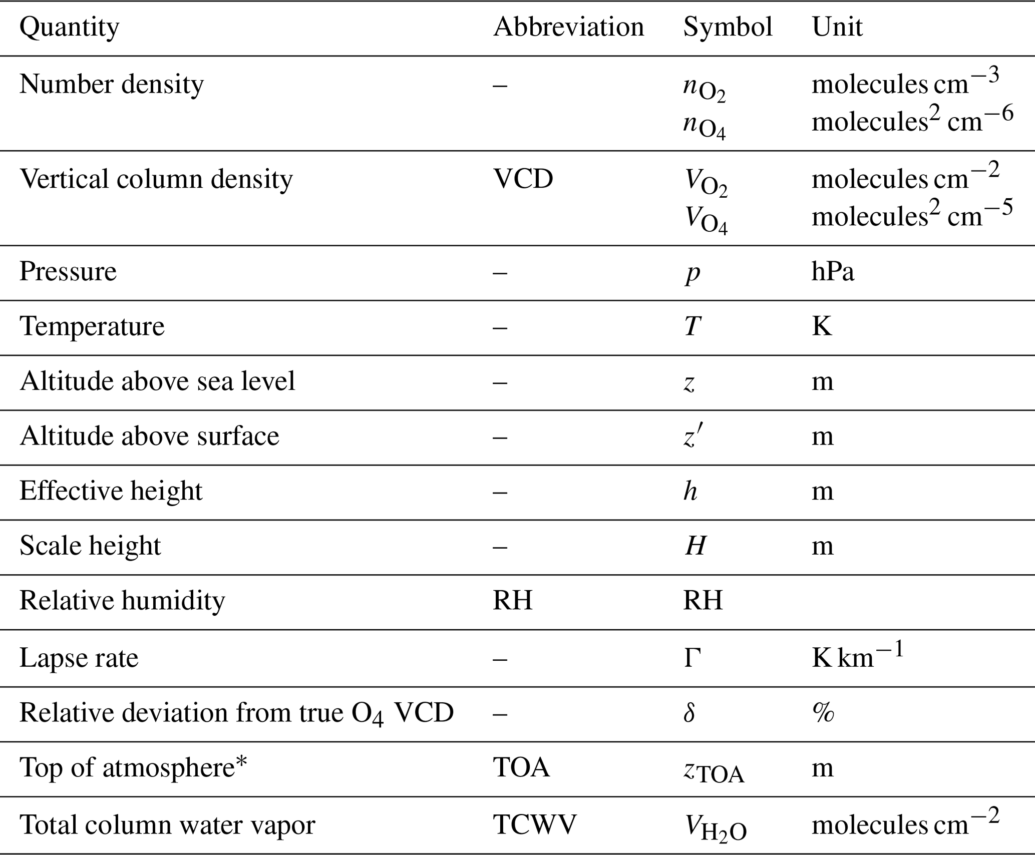
^* Here: highest available/possible profile layer.

Table 2 Constants used in this study. Numbers are listed with six digits.

^a From the Python module MetPy (May et al., 2021).
^b Latitudinal variations of g are below ±0.27 % and are neglected in this study.
^c From Tohjima et al. (2005).

2.2 General approach

The VCD V is the vertically integrated number density n:

$$\begin{array}{}\text{(1)}& V=\underset{z_{\mathrm{0}}}{\overset{\mathrm{\infty }}{\int }}n\left(z\right)\mathrm{d}z.\end{array}$$

This integral can be re-written as

$$\begin{array}{}\text{(2)}& V=n_{\mathrm{0}}\cdot h,\end{array}$$

with

$$\begin{array}{}\text{(3)}& h=\underset{z_{\mathrm{0}}}{\overset{\mathrm{\infty }}{\int }}{\displaystyle \frac{n\left(z\right)}{n_{\mathrm{0}}}}\mathrm{d}z.\end{array}$$

This effective height h can be understood as the height of the gas column if the gas would be in a homogenous box under surface conditions p₀ and T₀. Note that the effective height equals the scale height H only in the case of exponential profiles, i.e., an isothermal atmosphere (see Appendix A).

Thus, the VCDs for O₂ and O₄ can be written as

$$\begin{array}{}\text{(4)}& V_{{\text{O}}_{\mathrm{2}}}=n_{{\text{O}}_{\mathrm{2}},\mathrm{0}}\cdot h_{{\text{O}}_{\mathrm{2}}},\end{array}$$

and

$$\begin{array}{}\text{(5)}& V_{{\text{O}}_{\mathrm{4}}}=n_{{\text{O}}_{\mathrm{4}},\mathrm{0}}\cdot h_{{\text{O}}_{\mathrm{4}}}=n_{{\text{O}}_{\mathrm{2}},\mathrm{0}}^{\mathrm{2}}\cdot h_{{\text{O}}_{\mathrm{4}}}.\end{array}$$

Re-arranging Eq. (4) for $n_{{\text{O}}_{\mathrm{2}},\mathrm{0}}$ and replacing one $n_{{\text{O}}_{\mathrm{2}},\mathrm{0}}$ term in Eq. (5) yields

$$\begin{array}{}\text{(6)}& V_{{\text{O}}_{\mathrm{4}}}=V_{{\text{O}}_{\mathrm{2}}}\cdot n_{{\text{O}}_{\mathrm{2}},\mathrm{0}}\cdot {\displaystyle \frac{h_{{\text{O}}_{\mathrm{4}}}}{h_{{\text{O}}_{\mathrm{2}}}}}.\end{array}$$

Hence the O₄ VCD can be expressed as the product of the O₂ VCD, the O₂ surface number density, and the ratio of effective heights of O₂ and O₄ profiles. So far, no simplifications or approximations have been made; thus Eq. (6) holds for any atmospheric conditions.

2.3 O₄ VCD as a function of surface pressure, surface temperature, and lapse rate

Based on Eq. (6), the O₄ VCD can be related to surface pressure, surface temperature, and lapse rate, if some further assumptions are made:

1. Assuming a hydrostatic atmosphere, the surface pressure is just the gravitational force per area of the total air column. Thus, the O₂ VCD is directly related to the surface pressure:

   $$\begin{array}{}\text{(7)}& V_{{\text{O}}_{\mathrm{2}}}={\displaystyle \frac{{\mathit{\nu }}_{{\text{O}}_{\mathrm{2}}}}{g\cdot M}}\cdot p_{\mathrm{0}},\end{array}$$

   with ${\mathit{\nu }}_{{\text{O}}_{\mathrm{2}}}$ being the volume mixing ratio of O₂ in dry air, g being the gravitational acceleration on Earth, and M being the molar mass of dry air.

2. According to the ideal gas law for dry air, the surface number density of O₂ can be expressed as

   $$\begin{array}{}\text{(8)}& n_{{\text{O}}_{\mathrm{2}},\mathrm{0}}={\displaystyle \frac{{\mathit{\nu }}_{{\text{O}}_{\mathrm{2}}}}{R}}\cdot {\displaystyle \frac{p_{\mathrm{0}}}{T_{\mathrm{0}}}},\end{array}$$

   with the universal gas constant R.

3. The ratio of effective heights for O₂ and O₄ depends on the actual profile shape for O₂. For some specific cases, the integral in Eq. (3) can be solved analytically (see Appendix A for details):

   • For an isothermal atmosphere, i.e., an exponential profile of $n_{{\text{O}}_{\mathrm{2}}}$, the ratio $\frac{h_{{\text{O}}_{\mathrm{2}}}}{h_{{\text{O}}_{\mathrm{4}}}}$ is just 2 (Eq. A2).

   • For a constant lapse rate Γ, the ratio becomes $\mathrm{2}+\frac{R}{g\cdot M}\mathrm{\Gamma }$ (Eq. A10).

   • For real atmospheric conditions, where the lapse rate varies with altitude, the ratio of effective heights can be still described by Eq. (A10) if an effective lapse rate is considered:

     $$\begin{array}{}\text{(9)}& {\mathrm{\Gamma }}_{\text{eff}}:=({\displaystyle \frac{h_{{\text{O}}_{\mathrm{2}}}}{h_{{\text{O}}_{\mathrm{4}}}}}-\mathrm{2})\cdot {\displaystyle \frac{g\cdot M}{R}}.\end{array}$$

     For a given atmospheric profile, the effective lapse rate is thus defined as the lapse rate of a polytropic atmosphere of the same O₄ VCD.

Replacing the terms in Eq. (6) by Eqs. (7), (8) and (A10) yields

$$\begin{array}{}\text{(10)}& \begin{array}{rl}{V}_{{\text{O}}_{\mathrm{4}},\mathrm{\Gamma }}& ={\displaystyle \frac{{\mathit{\nu }}_{{\text{O}}_{\mathrm{2}}}^{\mathrm{2}}}{R\cdot g\cdot M}}/(\mathrm{2}+{\displaystyle \frac{R}{g\cdot M}}\mathrm{\Gamma })\cdot {\displaystyle \frac{p_{\mathrm{0}}^{\mathrm{2}}}{T_{\mathrm{0}}}}\\ & ={\displaystyle \frac{C}{\mathrm{2}+\frac{R}{g\cdot M}\mathrm{\Gamma }}}\cdot {\displaystyle \frac{p_{\mathrm{0}}^{\mathrm{2}}}{T_{\mathrm{0}}}}\end{array}\end{array}$$

with

$$\begin{array}{}\text{(11)}& C={\displaystyle \frac{{\mathit{\nu }}_{{\text{O}}_{\mathrm{2}}}^{\mathrm{2}}}{R\cdot g\cdot M}}\end{array}$$

combining the constant factors. Thus with the assumptions specified above, the O₄ VCD is proportional to $p_{\mathrm{0}}^{\mathrm{2}}/T_{\mathrm{0}}$, with the lapse rate Γ determining the slope.

2.4 Calculation of the “true” O₄ VCD

In order to evaluate the performance of the parameterizations for the O₄ VCD, we also calculate the “true” O₄ VCD, which is derived by (a) calculating the profile of $n_{{\text{O}}_{\mathrm{2}}}$ from profiles of T, p, and RH. In this step, the effect of humidity is explicitly accounted for by subtracting the water vapor pressure before calculating $n_{{\text{O}}_{\mathrm{2}}}$ based on the ideal gas law, (b) performing the numerical integration (using Simpson's rule) of $n_{{\text{O}}_{\mathrm{2}}}^{\mathrm{2}}$ from surface to top of atmosphere (TOA).

The integration has to be performed up to sufficiently high altitudes (Wagner et al., 2019 recommend z_TOA≥30 km) as otherwise the integrated VCD would be biased low due to the missing column above. As not all datasets considered below cover this altitude range, we estimate and correct for the missing O₄ column above the highest profile level by applying Eq. (10) for the highest available layer, assuming a lapse rate of zero above. Note that the temperature increase in the upper stratosphere is not relevant here as the contribution to the O₄ VCD above 30 km is negligible. Thus, the “true” O₄ VCD is calculated as

$$\begin{array}{}\text{(12)}& V_{{\text{O}}_{\mathrm{4}},\text{true}}=\underset{z_{\mathrm{0}}}{\overset{z_{\text{TOA}}}{\int }}{n}_{{\text{O}}_{\mathrm{2}}}^{\mathrm{2}}\left(z\right)\mathrm{d}z+{\displaystyle \frac{C}{\mathrm{2}}}\cdot {\displaystyle \frac{p_{\text{TOA}}^{\mathrm{2}}}{T_{\text{TOA}}}}.\end{array}$$

For z_TOA of 20 km, the correction term is of the order of 0.3 % of the total O₄ column.

2.5 O₄ VCD as a function of surface pressure, surface temperature, and surface relative humidity

Equation (10) might be applied for a common lapse rate, like −6.5 K km⁻¹ as proposed in Wagner et al. (2019). This works generally well over most continental regions. However, large deviations have to be expected for regions with different lapse rates, in particular over deserts, where lapse rates are typically stronger (more negative, i.e., close to the dry adiabatic lapse rate). Over parts of the ocean, on the other hand, lapse rates are weaker (closer to zero).

In order to modify Eq. (10) such that it can be applied globally, but keep it still a simple function of surface measurements, we make use of the relation between the effective lapse rate and the RH at ground:

• For ascending air masses, RH₀ determines the altitude at which condensation takes place. This relation is directly reflected in the calculation of the lifted condensation level (LCL) as function of RH₀ (Lawrence, 2005; Romps, 2017). Thus, the lower RH₀, the higher the altitude range above ground where dry adiabatic lapse rates apply.

• For descending air masses (in particular the large-scale subsidence over tropical deserts), no condensation takes place and dry adiabatic lapse rates apply.

In both cases, low relative humidity at ground is associated with lapse rates closer to the dry adiabatic lapse rate.

Real atmospheric profiles are of course more complex than these simplified scenarios, in particular due to advection, but still, a correlation between RH₀ and effective lapse rates is expected. We thus parameterize the effective lapse rate by the relative humidity at ground via a linear function:

$$\begin{array}{}\text{(13)}& {\mathrm{\Gamma }}_{\text{eff}}=\mathit{\alpha }+\mathit{\beta }\cdot {\text{RH}}_{\mathrm{0}}.\end{array}$$

Replacing this in Eq. (10) results in $V_{{\text{O}}_{\mathrm{4}}}$ becoming a function of surface values for pressure, temperature, and relative humidity:

$$\begin{array}{}\text{(14)}& \begin{array}{rl}{V}_{{\text{O}}_{\mathrm{4}},\text{RH}}& ={\displaystyle \frac{C}{\mathrm{2}+\frac{R}{g\cdot M}\cdot (\mathit{\alpha }+\mathit{\beta }\cdot {\text{RH}}_{\mathrm{0}})}}\cdot {\displaystyle \frac{p_{\mathrm{0}}^{\mathrm{2}}}{T_{\mathrm{0}}}}\\ & ={\displaystyle \frac{C}{a+b\cdot {\text{RH}}_{\mathrm{0}}}}\cdot {\displaystyle \frac{p_{\mathrm{0}}^{\mathrm{2}}}{T_{\mathrm{0}}}},\end{array}\end{array}$$

where the parameters a and b are linked to α and β from Eq. (13) via

$$\begin{array}{}\text{(15)}& \mathit{\alpha }=(a-\mathrm{2})\cdot {\displaystyle \frac{g\cdot M}{R}}\end{array}$$

and

$$\begin{array}{}\text{(16)}& \mathit{\beta }={\displaystyle \frac{g\cdot M}{R}}\cdot b.\end{array}$$

The parameters a and b can then be determined by a linear least squares fit by comparing $V_{{\text{O}}_{\mathrm{4}},\text{RH}}$ to $V_{{\text{O}}_{\mathrm{4}},\text{true}}$:

$$\begin{array}{}\text{(17)}& V_{{\text{O}}_{\mathrm{4}},\text{RH}}={\displaystyle \frac{C}{a+b\cdot {\text{RH}}_{\mathrm{0}}}}\cdot {\displaystyle \frac{p_{\mathrm{0}}^{\mathrm{2}}}{T_{\mathrm{0}}}}\stackrel{!}{=}{V}_{{\text{O}}_{\mathrm{4}},\text{true}};\end{array}$$

thus

$$\begin{array}{}\text{(18)}& a+b\cdot {\text{RH}}_{\mathrm{0}}\stackrel{!}{=}{\displaystyle \frac{C}{V_{{\text{O}}_{\mathrm{4}},\text{true}}}}\cdot {\displaystyle \frac{p_{\mathrm{0}}^{\mathrm{2}}}{T_{\mathrm{0}}}}=:Q.\end{array}$$

a and b will be derived in Sect. 4.2 based on true O₄ VCDs calculated from ECMWF profiles. This empirical approach also, at least partly, corrects for effects neglected in the derivation of Eq. (10), i.e., ignoring the tropopause in the calculation of the ratio of effective heights (Appendix A3), and applying the ideal gas law for dry air in Sect. 2.3.

From a and b, also the corresponding effective lapse rate for a given RH₀ can then be calculated with Eqs. (13), (15), and (16). This lapse rate allows one to construct full atmospheric profiles of T and p (applying the barometric formula for polytropic atmosphere) from surface measurements when needed, in particular for MAX-DOAS inversions based on optimal estimation. As humidity effects are already accounted for in the determination of a and b, no further correction for humidity should be applied in this case.

2.6 Comparison of parameterized to “true” O₄ VCD

In order to assess accuracy and precision of the proposed calculation of the O₄ VCD from surface measurements of T₀, p₀, and Γ (Eq. 10) or RH₀ (Eq. 14), we define the relative deviation δ of a derived O₄ VCDs to the true value:

$$\begin{array}{}\text{(19)}& {\mathit{\delta }}_x={\displaystyle \frac{V_{{\text{O}}_{\mathrm{4}},x}-V_{{\text{O}}_{\mathrm{4}},\text{true}}}{V_{{\text{O}}_{\mathrm{4}},\text{true}}}}.\end{array}$$

The index x indicates the O₄ VCD dataset and is “Γ” for $V_{{\text{O}}_{\mathrm{4}},\mathrm{\Gamma }}$ and “RH” for $V_{{\text{O}}_{\mathrm{4}},\text{RH}}$.

3 Datasets

For illustration as well as for the quantification of uncertainties, we apply the derived formalism to different atmospheric datasets:

1. global model data, in order to check for the performance of the parameterizations globally, covering the full range of the relevant parameter space for surface values of pressure, temperature, humidity, and altitude;

2. regional model data with high spatial resolution, which are also compared to surface stations and allow the investigation of the impact of diurnal cycles;

3. balloon-borne radiosonde measurements, in order to apply the formalism to high-resolved profile measurements.

Nighttime profiles of T can be considerably different from daytime profiles, in particular in the case of temperature inversions (i.e., positive lapse rates) often occurring within the nocturnal boundary layer. For MAX-DOAS measurements, however, nighttime profiles are irrelevant. Thus, we consider all atmospheric datasets for daytime conditions only. This is done by selecting data with an solar zenith angle (SZA) below 85^∘.

3.1 Global model (ECMWF)

We use global model data as provided by the European Centre for Medium-Range Weather Forecasts (ECMWF) for two purposes:

• In order to investigate global patterns, we use ERA5 reanalysis data (Hersbach et al., 2020) truncated at wavenumber 639 on the Gaussian grid N320, corresponding to ≈0.3^∘ resolution. Model output is provided hourly. Here, we focus on ERA5 data for four selected days, i.e., 18 March, 18 June, 18 September, and 18 December 2018, covering the full globe for all seasons. As the regular latitude–longitude grid over-represents high latitudes, we only consider the fraction of cos(lat) pixels for each latitude for the calculation of histograms, correlation coefficients, means, and standard deviations.

• For comparison with the standard approach for the calculation of the O₄ VCD that was used in MAPA so far, we use ERA-Interim reanalysis data truncated at wavenumber 255, corresponding to ≈0.7^∘ resolution, which was preprocessed to a dataset with 6 hourly model output (00:00, 06:00, 12:00, 18:00 UTC) interpolated to a regular horizontal grid with a resolution of 1^∘. This dataset is denoted as ERA_I_daily below.

  In addition, we make use of a monthly climatology of atmospheric profiles (ERA_I_clim) based on the same ERA-Interim data, which was constructed as back-up solution recommended within the FRM4DOAS project in case no other profile information is available.

3.2 Regional model (WRF-Chem) and surface measurements (DWD)

We use the Weather Research and Forecasting (WRF) model version 4.2 (Skamarock et al., 2019) for high-resolution (3×3 km²) simulations of meteorological parameters (including T, p, and RH) around Germany for May and June 2018. Further details on the WRF model setup are provided in Appendix B1.1.

WRF simulations of surface values are also compared to surface measurements performed by Germany's National Meteorological Service (Deutscher Wetterdienst, DWD). For further details see Appendix B1.2 and B1.3.

3.3 Radiosonde measurements (GRUAN)

The Global Climate Observing System (GCOS) Reference Upper-Air Network (GRUAN) is an international reference observing network of sites measuring essential climate variables above Earth's surface (Sommer et al., 2012; Bodeker et al., 2016). Atmospheric profiles of temperature, pressure, and humidity are measured by regular balloon soundings equipped with radiosondes and water vapor measurements (Dirksen et al., 2014). Here we use the RS92 GRUAN Data Product Version 2 (RS92-GDP.2), focusing on certified stations. Vertical profiles and surface values of pressure, temperature, and relative humidity are taken directly from the level-2 files for each launch. Further information on the GRUAN stations used in this study is provided in Appendix B2.

4 Application to atmospheric datasets

In this section, we apply the parameterizations of the O₄ VCD derived in Sect. 2 to modeled and measured atmospheric datasets, and we assess the accuracy and precision of the different parameterizations by comparison to the true O₄ VCD (Sect. 2.4). We first present O₄ VCDs based on an a priori lapse rate in Sect. 4.1, discuss the relation between effective lapse rate and surface humidity in Sect. 4.2, and finally present O₄ VCDs based on RH₀ in Sect. 4.3.

4.1 O₄ VCD as a function of p₀, T₀, and lapse rate Γ

According to Eq. (10), the O₄ VCD is proportional to $p_{\mathrm{0}}^{\mathrm{2}}/T_{\mathrm{0}}$, with the lapse rate Γ determining the slope. We illustrate this correlation for the investigated datasets in Fig. 1.

Figure 1 Density plots of the relation between the O₄ VCD and $p_{\mathrm{0}}^{\mathrm{2}}/T_{\mathrm{0}}$ for (a) WRF data for May to June 2018 from 07:00 to 17:00 UTC, (b) ERA5 data for the 4 selected days in 2018, and (c) all available GRUAN profiles. Frequency per pixel is color coded, with a binning of 100 pixels for both x and y axis, as in all 2D frequency distributions shown below. Respective correlation coefficients are provided in the top right of each panel. Lines display the expected dependency according to Eq. (10) for different lapse rates. Low values correspond to high-altitude sites with low surface pressure; for GRUAN, only few of such stations are available (Boulder and La Réunion at 1.7 and 2.2 km altitude, respectively). The very high values for ERA5 and GRUAN are observed for polar regions with cold temperatures.

$V_{{\mathrm{O}}_{\mathrm{4}},\mathrm{true}}$ varies considerably for all datasets, where the low values are caused by mountains due to reduced pressure, while the very high values for ERA5 and GRUAN are caused by cold temperatures in polar regions. The variability of $V_{{\mathrm{O}}_{\mathrm{4}},\mathrm{true}}$ is well reflected in $p_{\mathrm{0}}^{\mathrm{2}}/T_{\mathrm{0}}$, and very good correlation between both quantities is found, with most data points in accordance with plausible lapse rates in the range of −4 to −6.5 K km⁻¹. For the WRF simulations for Germany, most data points match a lapse rate close to −6.5 K km⁻¹. ERA5 and GRUAN data show higher variability in slopes, as they also cover a wider range of atmospheric conditions.

Wagner et al. (2019) proposed to determine the O₄ VCD based on vertical profiles of T and p constructed from the respective surface values by assuming a constant tropospheric lapse rate of −6.5 K km⁻¹. We can use Eq. (10) for the same purpose, but without the need for constructing full vertical profiles. Figures 2 and 3 display maps of the deviation δ_Γ between parameterized and true O₄ VCD for WRF and ERA5, respectively, assuming a constant lapse rate of −6.5 K km⁻¹. Results for additional days for ERA5 are shown in Appendix C.

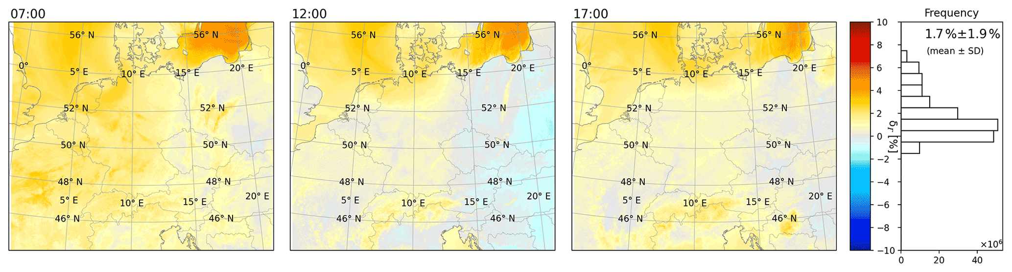
Figure 2 Deviation δ_Γ according to Eq. (19) for WRF simulations at 07:00, 12:00, and 17:00 UTC on 1 May 2018. On the right, the frequency distribution of δ_Γ and its mean and SD are given for the WRF simulation period from May to June 2018.

Generally, good agreement between $V_{{\text{O}}_{\mathrm{4}},\mathrm{\Gamma }}$ and $V_{{\mathrm{O}}_{\mathrm{4}},\mathrm{true}}$ is found (Fig. 2): on average, δ_Γ is 1.7 %; i.e., $V_{{\text{O}}_{\mathrm{4}},\mathrm{\Gamma }}$ are higher than $V_{{\mathrm{O}}_{\mathrm{4}},\mathrm{true}}$ by 1.7 %. Over land around noon, δ_Γ is close to 0. Over ocean, however, δ_Γ is higher (about 3 % up to 7 %).

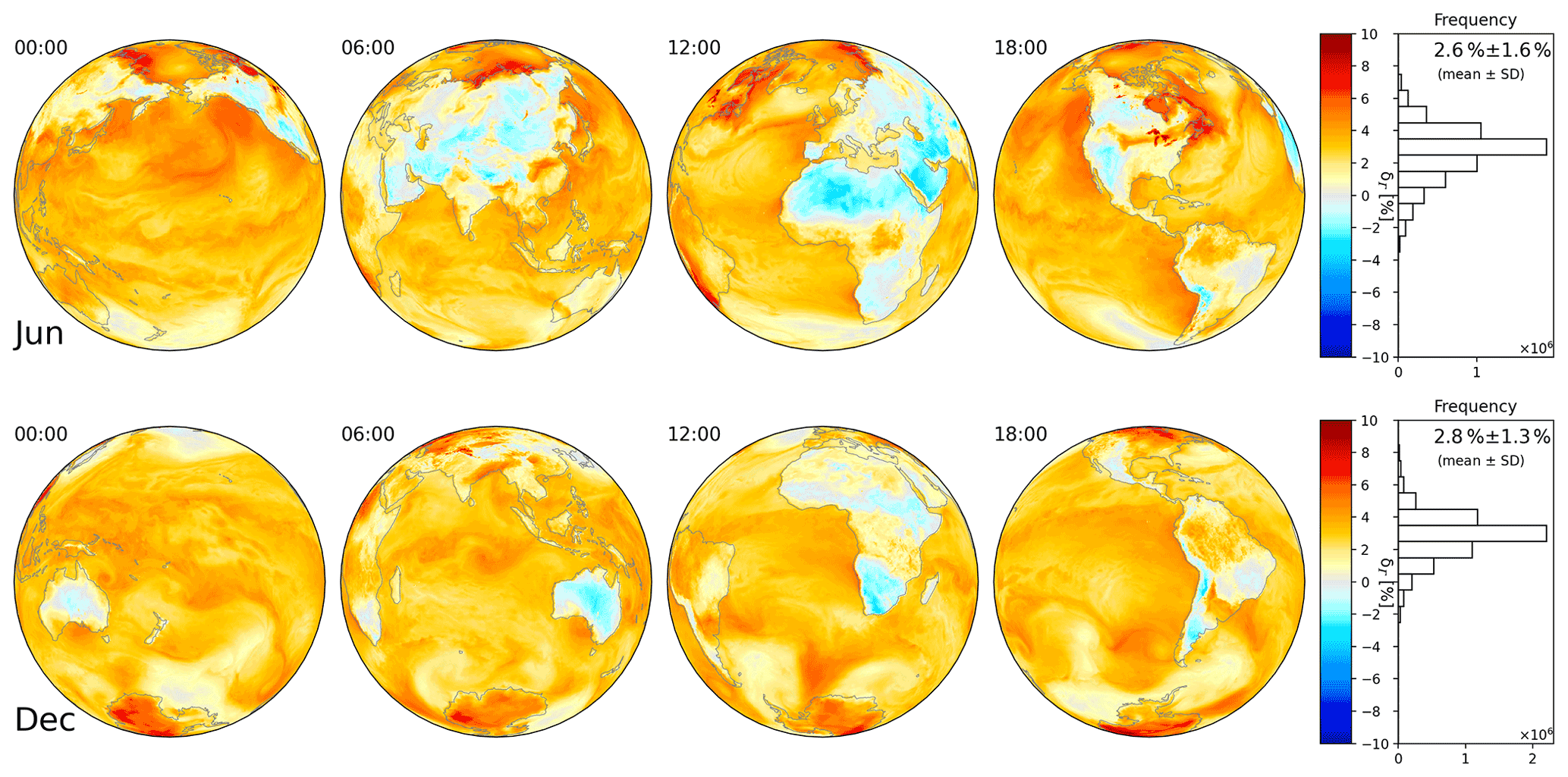
Figure 3 Deviation δ_Γ according to Eq. (19) for ERA5 at 00:00, 06:00, 12:00, and 18:00 UTC on 18 June (top) and 18 December (bottom) 2018. The projection focuses on daytime for each time step. On the right, the frequency distribution and mean and SD are given for all hourly outputs of the respective day. Results for 18 March and 18 September 2018 are shown in Fig. C1.

For ERA5 data on 18 June 2018, δ_Γ over Germany is close to 0 as well (Fig. 3). On a global scale, however, only moderate agreement is found between $V_{{\text{O}}_{\mathrm{4}},\mathrm{\Gamma }}$ and $V_{{\mathrm{O}}_{\mathrm{4}},\mathrm{true}}$, with a mean deviation of 2.6 %. High values for δ_Γ are found generally over ocean. In particular over cold water surfaces, like the west coast of North America and South America, the Hudson Bay, or the Great Lakes, δ_Γ is very high (up to 7 %). This is related to temperature inversions close to ground: due to the too low surface temperatures (as compared to a polytropic atmosphere with the same O₄ VCD), the O₄ VCD calculated from Eq. (10) is biased high. This will be discussed in detail in Sect. 5.2. Over continents, δ_Γ is lower, and generally close to 0, except over deserts, where negative values are observed.

4.2 Effective lapse rate and relative humidity at ground

Figure 4 displays the effective lapse rate, as defined in Eq. (9), for ERA5 data from 18 June 2018, clearly showing that the general patterns of systematic deviations seen in Fig. 3 are mainly caused by the simple assumption of a globally constant lapse rate in the calculation of δ_Γ.

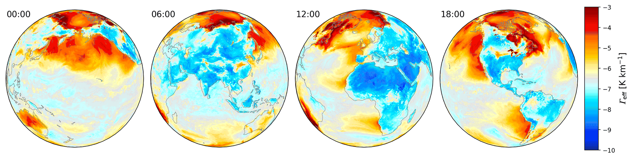
Figure 4 Effective lapse rate Γ_eff as defined in Eq. (9) for ERA5 profiles on 18 June 2018.

In Fig. 5a, the effective lapse rate is compared to the actual lapse rate between ground and 5 km altitude above ground, revealing a correlation of 0.83. Figure 5b displays the relation between relative humidity at ground and the effective lapse rate (R=0.59). Assuming a linear relation between Γ_eff and RH₀ in Eq. (13) results in a linear relation between RH₀ and the ratio Q (Eq. 18). This is displayed in Fig. 5c. Interestingly, the correlation (R=0.79) is far better than in (b) (R=0.59). This indicates that the parameterization based on RH₀ at least partly corrects for other simplifications made in the formalism in Sect. 2.3, in particular the neglect of humidity in the ideal gas law.

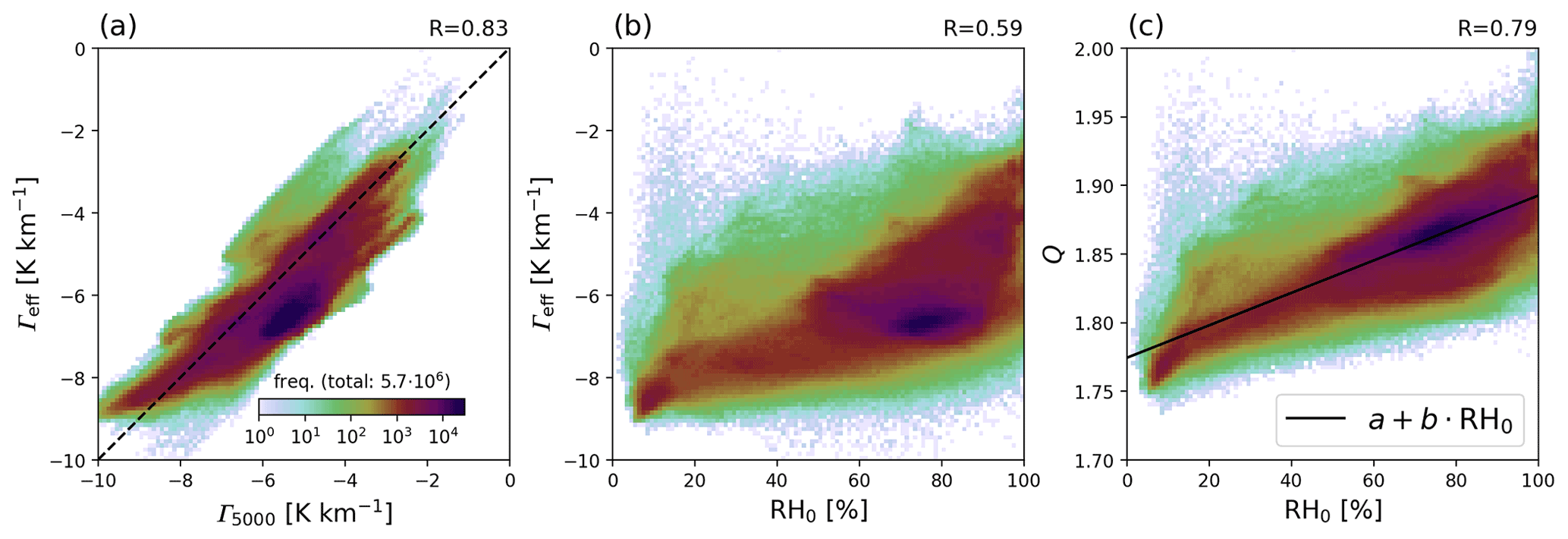
Figure 5 Relations between lapse rate, RH₀, and ratio Q for ERA5 data on 18 June 2018. (a) Relation between the actual lapse rate (calculated from the temperature difference between ground and 5 km altitude) and the effective lapse rate. (b) Relation between RH₀ and effective lapse rate. (c) Relation between RH₀ and the ratio Q as defined in Eq. (18), where the black line shows the linear fit $a+b\cdot {\text{RH}}_{\mathrm{0}}$.

We use ERA5 data from 18 June 2018 to determine the parameters a and b in Eq. (14) by applying a linear least squares fit to the data presented in Fig. 5c, as shown by the black line. Fitted parameters are $a=\mathrm{1.77434}\pm \mathrm{0.00003}$ and $b=\mathrm{0.11821}\pm \mathrm{0.00004}$ (for RH₀ in absolute numbers, i.e., 0.5 for 50 % RH). The corresponding parameterization of the effective lapse rate (Eq. 13) is ${\mathrm{\Gamma }}_{\text{eff}}=(-\mathrm{7.709}+\mathrm{4.038}\cdot {\text{RH}}_{\mathrm{0}})$ K km⁻¹, which yields −7.709, −5.690 and −3.671 K km⁻¹ for RH₀ of 0 %, 50 %, and 100 %, respectively.

4.3 O₄ VCD as function of p₀, T₀, and RH₀

With Eq. (14), an empirical parameterization of the O₄ VCD was derived based on surface values of temperature, pressure, and relative humidity. We applied this parameterization to all investigated datasets. Figures 6 and 7 display δ_RH for WRF and ERA5, respectively. GRUAN results are shown in Fig. 8.

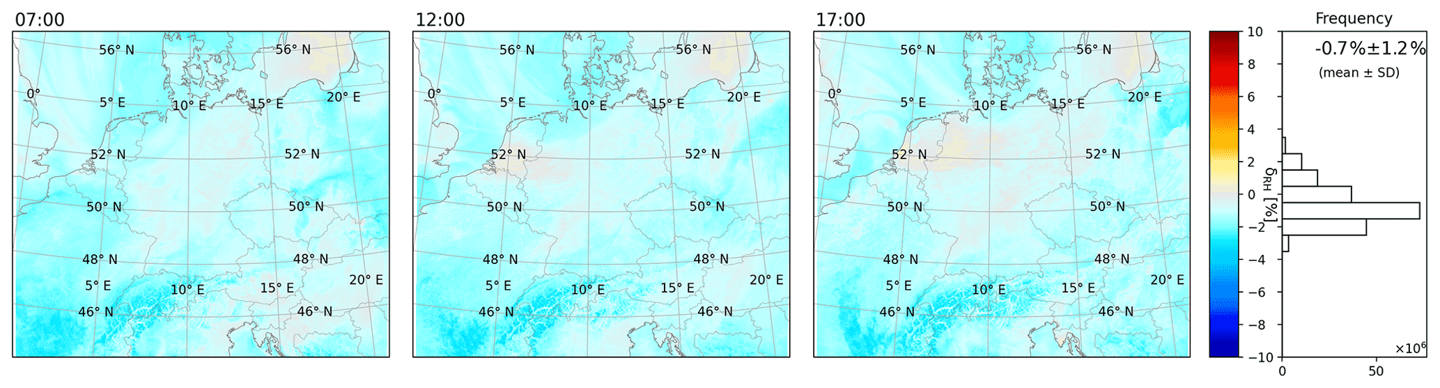
Figure 6 Deviation δ_RH according to Eq. (19) for WRF simulations at 07:00, 12:00, and 17:00 UTC on 1 May 2018. On the right, the frequency distribution and mean and SD are given for the WRF simulation period from May to June.

Figure 7 Deviation δ_RH according to Eq. (19) for ERA5 at 00:00, 06:00, 12:00, and 18:00 UTC on 18 June (top) and 18 December (bottom) 2018. The projection focuses on daytime for each time step. On the right, the frequency distribution and mean and SD are given for all hourly outputs of the respective day. Note that the mean deviation on 18 June 2018 is 0 by construction, as the parameters a and b (Eq. 14) are optimized for this day. Results for 18 March and 18 September 2018 are shown in Fig. C2.

For the WRF simulations, δ_Γ was already quite close to 0 (mean δ_Γ=1.6 %; see Fig. 2). δ_RH (Fig. 6) is closer to 0, but now showing a slight negative bias (mean ${\mathit{\delta }}_{\text{RH}}=-\mathrm{0.7}$ %). Variability has reduced considerably (SD of δ_RH is 1.2 %, compared to 1.9 % for δ_Γ). δ_RH shows a weaker land–ocean contrast. Over the Alps, δ_RH is biased low (down to −3 %).

For ERA5, the parameterization involving RH is a substantial improvement compared to the results for δ_Γ. The large difference between land (in particular deserts) and oceans seen in δ_Γ (Fig. 3) is strongly reduced for δ_RH (Fig. 7). For 18 June 2018, the mean of δ_RH≡0.0 % is of course a consequence of the fit optimizing a and b which is based on the same ERA5 dataset. But also for 18 December 2018, the mean deviation is close to zero. The SD reduces from 1.6 % for δ_Γ to 1.0 % for δ_RH on 18 June 2018, and from 1.3 % to 1.2 % on 18 December 2018. Applying Eq. (14) to ECMWF data from other months yields similar results, as shown in Fig. C2, with largest deviations of 0.2±1.8 % observed for 18 March 2018.

Remaining systematic deviations in the maps of δ_RH are due to

• weather, for instance associated with low pressure or frontal systems. This reflects the simplifying assumptions made, in particular assuming hydrostatic conditions in Sect. 2. Note, however, that MAX-DOAS retrievals are usually not considered for weather conditions associated with rain and clouds.

• cold surfaces causing temperature inversions, as discussed in more detail in Sect. 5.2.

• mountains, which tend to show systematic deviations δ_RH that are mostly negative (e.g., over the Andes or the Himalayas). For further discussion see Sect. 5.4.

• some patterns of enhanced δ_RH at the northern, southern, or western edge of the maps for ERA5, corresponding to polar regions as well as sampling times shortly after sunrise (e.g., over southern Africa at 06:00 UTC).

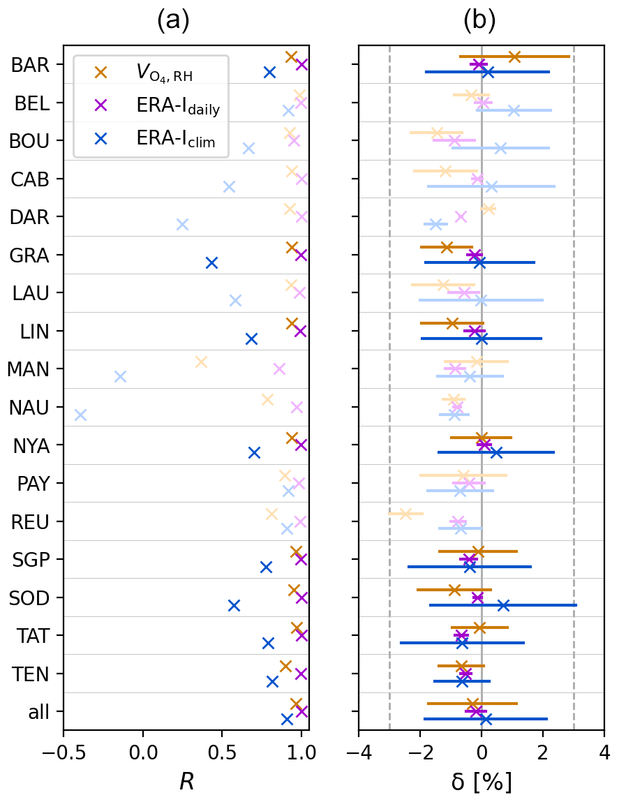
Figure 8 Comparison to the true O₄ VCD in terms of temporal correlation coefficient (a) and deviation δ according to Eq. (19) (b) for all GRUAN stations for O₄ VCDs calculated from (a) Eq. (14) based on GRUAN surface values (orange), (b) daily ERA-Interim profiles (purple) and (c) profiles from the ERA-Interim climatology (blue), interpolated to the GRUAN measurements in space and time. Light colors indicate stations with fewer than 100 profiles (compare Table B1).

So far, the formalism derived in Sect. 2 has been applied to data from meteorological models. Now we test it for measured profiles from radiosondes as well. Application of Eq. (14) to GRUAN data generally yields deviations close to 0 between parameterized and true O₄ VCDs for all stations, as shown in Fig. 8. Parameterized and true VCD show high correlations, indicating that the temporal variability of the atmospheric state is well captured by the simple parameterization based on surface values alone. The mean deviation δ_RH of all considered GRUAN profiles is −0.3 %, with a SD of 1.4 %. For 11 out of the 17 stations, the mean agreement is within 1 %. Largest deviations are found for La Réunion (REU), where $V_{{\text{O}}_{\mathrm{4}},\text{RH}}$ is biased low by −2.5 %. This is probably related to the altitude of this station of more than 2 km on a remote island in the Indian Ocean. Highest positive deviation of 1.1 % is found for Utqiaġvik, Alaska (formerly Barrow, which is the name used in the GRUAN dataset), with also highest SD of 1.8 %. This is caused by some very high values during spring where surface temperatures are very low (<240 K) and temperature inversions occur.

5 Discussion

5.1 Comparison to existing methods for the calculation of the O₄ VCD

Within MAPA (Beirle et al., 2019), the O₄ VCD has been so far determined by integrating vertical profiles of the O₄ number density based on full profiles of T, p, and RH, which are by default taken from daily ERA-Interim simulations (ERA-I_daily), or, as fallback solution, from a monthly climatology complied from multi-annual ERA-Interim data (ERA-I_clim), both on 1^∘ resolution.

Thus, we evaluate the performance of the proposed simple calculation of the O₄ VCD by comparing the results for GRUAN profiles, where the true O₄ VCD is known, also to the ERA-Interim profiles interpolated in space and time. In addition, a correction of surface altitude is necessary: for La Réunion, for instance, the radio sondes were launched at a surface altitude of 2 km, while the surface altitude in ERA-Interim (with 1^∘ resolution) is just 54 m. This could easily cause deviations of 10 % in O₄ VCDs when ignored. Thus we apply the following correction to the ERA-Interim profiles:

• In the case of GRUAN station altitude being higher than ERA-Interim surface altitude, the ERA-Interim profiles of T and RH are just linearly interpolated. As pressure profiles are almost exponential, ln (p) is linearly interpolated.

• In the case of GRUAN station altitude being lower than ERA-Interim surface altitude, ERA-Interim profiles are extended by surface values of T₀ and ln (p₀) as derived from linear extrapolation of T and ln (p), respectively. RH at ground, however, is not extrapolated, as this might result in unphysical values of RH below 0 or above 1. Instead, the value of the lowest ERA-Interim model layer is taken as RH₀.

We calculate the deviation from the true VCD (defined by the GRUAN profiles) according to Eq. (19) for daily and climatological ERA-Interim data. The correlation coefficients as well as mean and SD of the resulting deviations are also included in Fig. 8.

For O₄ VCDs based on daily ERA-Interim profiles, the agreement to VCDs integrated from GRUAN profiles is generally very good. Correlation coefficients are almost 1, and deviations are close to 0 for most stations. Only for mountainous sites such as Boulder, where surface altitude differs between GRUAN and ERA-Interim, clear deviations from 0 are found.

Results based on the ERA-Interim climatology, however, show far weaker correlation than for daily ERA-Interim data, as they do not resolve day-to-day changes in meteorology. Mean deviations are within ±1 % for most stations, with a SD of about 2 %.

In comparison to these existing methods, the O₄ VCDs based on Eq. (14) are worse than those based on daily ERA-Interim profiles but significantly better than those based on a profile climatology, in particular in terms of correlation and SD.

5.2 Impact of temperature inversions

The presented parameterizations derive the O₄ VCD just from surface values of T, p, and RH. This requires some basic assumptions about the atmospheric profile shape. In the case of temperature inversions, these assumptions do not hold. Thus, we focused on daytime conditions by selecting only data with $\text{SZA}<\mathrm{85}{}^{\circ }$. But still, temperature inversions can also occur during daytime, in particular over cold water and ice surfaces, as well as shortly after sunrise.

Figure 9 displays temperature inversions, here defined as the difference between tropospheric maximum and surface temperature, for ERA5 data on 18 June 2018. Strong temperature inversions are found, e.g., over Hudson Bay or the Great Lakes where sea surface temperature is low. Also at the western edge of the illuminated Earth (i.e., shortly after sunrise), temperature inversions occur, e.g., in northern and southern Africa at 06:00 UTC, indicating remnants of nocturnal profiles.

Large parts of the regions with high positive deviation δ_Γ (Fig. 3) or δ_RH (Fig. 7) actually correspond to temperature inversions. Thus, for MAX-DOAS measurements close to cold surface waters or other regions with temperature inversions, the formalism of Eqs. (10) and (14) should only cautiously be applied, and corrections of surface temperature might be needed for better results.

As the impact of temperature inversions on δ_Γ is quite strong, we skip profiles with temperature inversions of more than 2 K for the investigation of the effects of humidity (Sect. 5.3) and surface altitude (Sect. 5.4) in order to avoid interference of different effects.

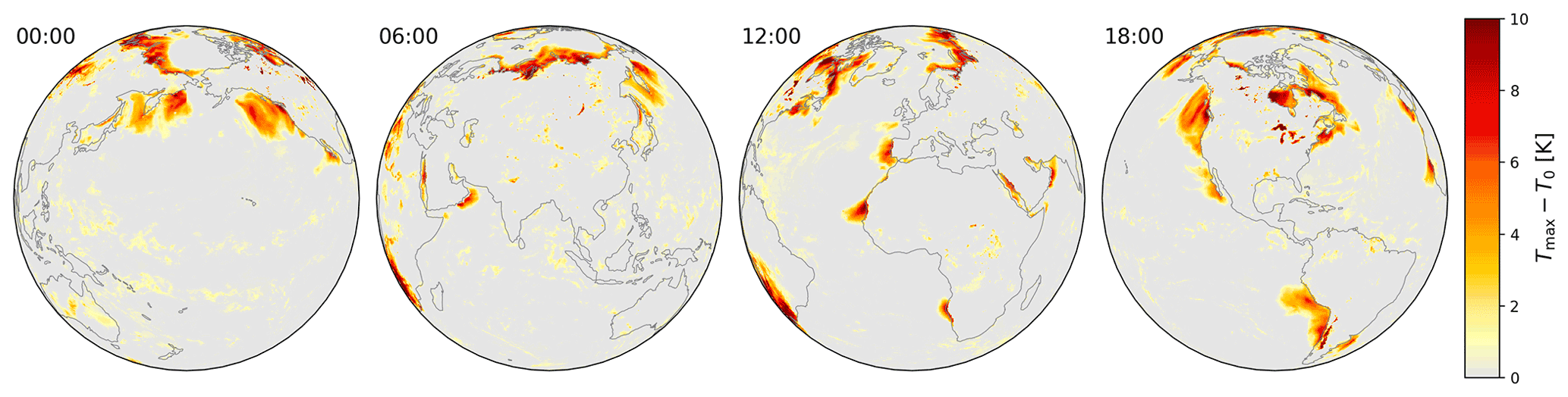
Figure 9 Temperature inversions, expressed as difference between tropospheric maximum and surface temperature, for ERA5 simulations at 00:00, 06:00, 12:00, and 18:00 UTC on 18 June 2018.

5.3 Impact of humidity

The formalism in Sect. 2.3 is assuming dry air. Addition of humidity results in lower O₂ and O₄ number densities, which significantly affects the O₄ VCD, especially in the tropics (Wagner et al., 2019). Humidity affects all terms in Eq. (6) (i.e., the O₂ VCD, the O₂ surface number density, and the ratio of effective heights of O₂ and O₄), but it cannot be accounted for in the formalism without completely losing the simplicity of Eq. (10).

However, these effects are partly accounted for in Eq. (14), with empirically determined parameters a and b, since the ratio Q was determined based on the true O₄ VCD where humidity effects were appropriately accounted for.

In order to check for possible remaining impacts of humidity on the performance of Eq. (14), we check how far δ_RH is related to specific humidity at ground (Fig. 10). In addition, we compare δ_RH also to the total column water vapor, as this provides information on humidity in the full column, not only at surface. In both cases, correlations are low, and no significant impact of humidity on δ_RH could be found.

Figure 10 Deviation δ_RH according to Eq. (19) as function of (a) specific humidity at ground, and (b) TCWV for ERA5 simulations on 18 June 2018. Temperature inversions with $T_{\text{max}}-T_{\mathrm{0}}>\mathrm{2}$ K have been skipped.

5.4 Impact of surface altitude

Figures 6 and 7 reveal systematic spatial patterns in δ_RH corresponding to mountains. We thus investigate a possible relation between surface altitude and δ_RH for all investigated datasets (Fig. 11).

Figure 11 Dependency of δ_RH on surface altitude for (a) WRF data for May to June 2018, (b) ERA5 data for all selected days, and (c) GRUAN data. For (b), temperature inversions with $T_{\text{max}}-T_{\mathrm{0}}>\mathrm{2}$ K have been skipped.

For the WRF simulations, the Alps can be clearly recognized in Fig. 6, with mountains showing lower values of δ_RH. This can also be seen in the density plot in Fig. 11a, where surface altitude and δ_RH are anticorrelated with $R=-\mathrm{0.46}$, and a decrease of δ_RH of roughly 1 % km⁻¹. For GRUAN stations (c), results are similar, but statistics are poor, and the correlation coefficient is low, as only two stations (Boulder and La Réunion) are available with a surface altitude above 1 km.

For ERA5, however, results are not as clear as those for WRF. The correlation coefficient is low, and for altitudes between 2 and 3 km, it looks like δ_RH is increasing rather than decreasing with altitude. And for very high surface altitudes as found over the Himalaya, δ_RH is still close to 0 and would not match the slope of 1 % km⁻¹ estimated for WRF.

The reason for the poor correlation between z₀ and δ_RH for ERA5 compared to the WRF results is not clear to us. Obviously, other factors would probably also have to be considered (season, SZA). But since there is no clear correlation, and a quantitative correction would rather worsen δ_RH instead of improving it for several mountain areas around the globe, we decided not to apply an explicit correction for surface altitude.

Consequently, the parameterization of Eq. (14) has higher uncertainties when applied for mountainous sites: for z₀>2 km, δ_RH is −0.5 % on average with a SD of 1.8 %. But still, the parameterized O₄ VCD matches the requirement of accuracy/precision better than 3 % even for elevated sites.

5.5 Diurnal cycles

Surface conditions can change rapidly, e.g., in the case of passing frontal systems or storm tracks. For such rapid changes, the change of the true O₄ VCD might not be adequately represented by the change of $V_{{\text{O}}_{\mathrm{4}},\text{RH}}$. These effects are reflected in the SD of deviations δ_RH for ERA5, WRF, and GRUAN.

In addition, surface values could change systematically during the day in the case of strong solar irradiation, causing a diurnal cycle of surface temperature and the O₄ VCD (Wagner et al., 2019). Thus we investigate the diurnal cycles of T₀, p₀, RH₀, and the respective O₄ VCDs $V_{{\text{O}}_{\mathrm{4}},\text{RH}}$ and $V_{{\mathrm{O}}_{\mathrm{4}},\mathrm{true}}$ in more detail, and we check how far (a) the WRF simulations reflect the actual diurnal cycles and (b) the parameterized O₄ VCDs based on surface values reflect the diurnal cycle of the true O₄ VCD. For this, we extract the WRF simulations at the locations of the DWD ground station network. In order to focus on strong diurnal patterns, we select at each station those days where the intra-day change of surface temperature, as recorded by DWD, exceeds 10 K.

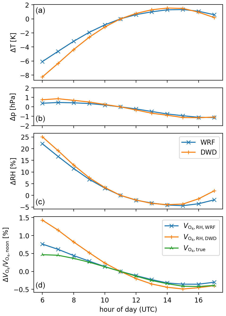
Figure 12 Diurnal cycles of surface temperature (a), pressure (b), RH (c), and the O₄ VCD (d). Data points show the mean values for all stations for May to June 2018 for days where the increase in T₀ (from DWD) over the day is larger than 10 K. For better comparison, the mean value at 11:00 UTC (around solar noon for Germany) is subtracted from all datasets. For the O₄ VCD, the relative change is shown.

Figure 12 displays the diurnal cycles of surface properties and O₄ VCDs for WRF and DWD station data. While surface pressure shows no relevant changes during day, surface temperature increases by 9.8 K from morning to afternoon due to the selection of days with strong diurnal cycle in surface temperature². For WRF simulations, a similar pattern is found, but the mean temperature increase over the day is smaller (7.4 K). As $V_{{\text{O}}_{\mathrm{4}},\text{RH}}$ is reciprocal to T₀, a change of 10 K in surface temperature alone would correspond to a change of $V_{{\text{O}}_{\mathrm{4}},\text{RH}}$ of 3.5 %. However, at the same time, RH decreases by about 30 %, which has an opposite effect on $V_{{\text{O}}_{\mathrm{4}},\text{RH}}$. Consequently, the diurnal cycle of $V_{{\text{O}}_{\mathrm{4}},\text{RH}}$ is only moderate (about 1.9 % and 1.1 % decrease from morning to evening for DWD and WRF, respectively, where the cycle for WRF is less strong due to the less strong cycle in T₀).

The true O₄ VCD, as derived from the integrated WRF profiles, also decreases over the day, and agrees well to $V_{{\text{O}}_{\mathrm{4}},\text{RH}}$ (WRF) in the afternoon. In the morning, however, $V_{{\text{O}}_{\mathrm{4}},\text{RH}}$ (WRF) is higher compared to noon by 0.8 %, while $V_{{\mathrm{O}}_{\mathrm{4}},\mathrm{true}}$ is only 0.5 % higher. This deviation between parameterized and true O₄ VCD indicates that in the early morning, surface measurements are not as useful for determining the full column, which is probably related to remainders of the nocturnal boundary layer which often has atypical lapse rates due to temperature inversions.

But even during morning hours, the systematic error made by $V_{{\text{O}}_{\mathrm{4}},\text{RH}}$ is relatively small, at least for the investigated time period for Germany. But also for the global ERA5 analysis, the impact of diurnal cycles on the calculation of the O₄ VCD is only moderate; otherwise, Figs. 7 and C2 would show systematic east–west gradients.

Thus, the parameterization of Eq. (14) also reflects most of the diurnal cycle of the O₄ VCD, with remaining systematic errors below 0.3 %.

5.6 Accuracy and precision

In Eq. (14), we provide a formula for the calculation of the O₄ VCD. Accuracy and precision of the resulting $V_{{\text{O}}_{\mathrm{4}}}$ thereby depend on accuracy and precision of (1) the chosen parameterization and (2) surface values p₀, T₀, and RH₀.

1. We estimate overall accuracy and precision of Eq. (14) to <1 % and <2 % based on mean and SD of deviations between parameterized and true O₄ VCD for WRF, ERA5 and GRUAN data as presented above. Higher deviations can occur in particular in the case of temperature inversions (see Sect. 5.2).

2. Application of Eq. (14) requires surface measurements of p₀, T₀, and RH₀. Uncertainties of temperature and pressure are rather uncritical, as an error of 1 K and 1 hPa for T₀ and p₀ would correspond to an error of 0.3 % and 0.2 % in $V_{{\text{O}}_{\mathrm{4}},\text{RH}}$, respectively. In order to reach an accuracy/precision of 1 %, the corresponding errors of RH₀ have to be lower than 16 %. These limits should be achievable for adequate meteorological instrumentation and a measurement procedure following World Meteorological Organization (WMO) guidelines. In particular, surface temperature should be measured at about 1.25 to 2 m above ground using a radiation shield (WMO, 2018).

The proposed parameterization thus allows one to calculate O₄ VCD with overall uncertainties below 3 %, which is sufficient for applications in MAX-DOAS profile inversions. Compared to existing methods, the parameterization yields even better results than a profile climatology.

We thus consider the proposed parameterization as a useful approach for determining the O₄ VCD for cases where no daily model profiles are available and recommend to also apply it for mountain sites for comparison and possible correction of daily model profiles.

6 Conclusions

The O₄ VCD can be expressed in terms of surface pressure and temperature based on physical laws, if a constant lapse rate is assumed, without the need for constructing full vertical profiles. With an empirical correction which parameterizes the effective lapse rate as linear function of surface RH, we could present a formula for simple and quick calculation of the O₄ VCD based on p₀, T₀, and RH₀:

$$\begin{array}{}\text{(20)}& V_{{\text{O}}_{\mathrm{4}},\text{RH}}={\displaystyle \frac{\mathrm{6.733}\times {\mathrm{10}}^{\mathrm{39}}}{\mathrm{1.774}+\mathrm{0.1182}\cdot {\text{RH}}_{\mathrm{0}}}}\cdot {\displaystyle \frac{p_{\mathrm{0}}^{\mathrm{2}}}{T_{\mathrm{0}}}}{\mathrm{molecules}}^{\mathrm{2}}{\mathrm{cm}}^{-\mathrm{5}}.\end{array}$$

This parameterization reproduces the real O₄ VCD, as derived from vertically integrated profiles, within $-\mathrm{0.7}\pm \mathrm{1.2}$ % for WRF simulations around Germany, 0.2±1.8 % for global reanalysis data (ERA5), and $-\mathrm{0.3}\pm \mathrm{1.4}$ % for radiosonde soundings around the world. Largest deviations are observed in the case of temperature inversions which cause too low T₀ (compared to the remaining profile) and thus high biased estimates of $V_{{\text{O}}_{\mathrm{4}},\text{RH}}$. For applications to measured surface values, uncertainties of 1 K, 1 hPa, and 16 % for temperature, pressure, and RH correspond to relative uncertainties of the O₄ VCD of 0.3 %, 0.2 %, and 1 %, respectively.

This accuracy and precision of <3 % is typically lower than other uncertainties of spectral analysis or radiative transfer modeling (Wagner et al., 2019). Thus, the proposed parameterization is well suited for application in MAX-DOAS profile inversions. Moreover, the parameterization reflects the true O₄ VCD, as derived from radiosonde measurements, even better (in particular in terms of temporal correlation and SD) than O₄ VCD calculated from a climatology of atmospheric profiles of T, p, and RH. We thus recommend to equip MAX-DOAS measurement stations with a state-of-the-art thermometer (with radiation shield), barometer, and hygrometer.

Appendix A: Ratio of effective heights

The ratio of the effective heights for O₄ and O₂ in Eq. (6) depends on the shape of the O₂ profile. For specific shapes the ratio can be calculated explicitly. Below, we derive the ratio $\frac{h_{{\text{O}}_{\mathrm{2}}}}{h_{{\text{O}}_{\mathrm{4}}}}$, which allows for simpler notation avoiding compound fractions. For application in Eq. (6), the inverse ratio has to be taken.

A1 Isothermal atmosphere

For the simple assumption of a barometric pressure profile with constant T, the O₂ number density decreases exponentially with altitude:

$$\begin{array}{}\text{(A1)}& n_{{\text{O}}_{\mathrm{2}}}=n_{{\text{O}}_{\mathrm{2}},\mathrm{0}}\cdot \exp \left(-z^{\prime }/H\right),\end{array}$$

with the scale height H. In this case, the integral of Eq. (3) directly yields H; i.e., the effective height equals the scale height for exponential profiles. For O₄, the profile is exponentially decreasing as well, with the scale height being half of that for O₂. Thus, for O₂ profiles declining exponentially with z, the ratio of effective heights is just

$$\begin{array}{}\text{(A2)}& {\displaystyle \frac{h_{{\text{O}}_{\mathrm{2}}}}{h_{{\text{O}}_{\mathrm{4}}}}}=\mathrm{2}.\end{array}$$

A2 Polytropic atmosphere

If the temperature is changing linearly with altitude, i.e., the dependence of $T\left(z\right)=T_{\mathrm{0}}+\mathrm{\Gamma }\cdot (z-z_{\mathrm{0}})$ is described by a constant lapse rate Γ, the resulting profile of O₂ follows a power function:

$$\begin{array}{}\text{(A3)}& n_{{\text{O}}_{\mathrm{2}}}=n_{{\text{O}}_{\mathrm{2}},\mathrm{0}}\cdot {\left(\mathrm{1}+{\displaystyle \frac{\mathrm{\Gamma }}{T_{\mathrm{0}}}}{z}^{\prime }\right)}^{-\mathit{\alpha }},\end{array}$$

with

$$\begin{array}{}\text{(A4)}& z^{\prime }=z-z_{\mathrm{0}}\end{array}$$

being altitude above surface, and

$$\begin{array}{}\text{(A5)}& \mathit{\alpha }=\mathrm{1}+{\displaystyle \frac{g\cdot M}{R\cdot \mathrm{\Gamma }}}\end{array}$$

being the constant exponent.

Note that for a constant lapse rate, temperature reaches 0 K at an altitude of

$$\begin{array}{}\text{(A6)}& z_{\text{TOA}}={\displaystyle \frac{T_{\mathrm{0}}}{\mathrm{\Gamma }}}.\end{array}$$

For T₀=300 K and $\mathrm{\Gamma }=-\mathrm{6.5}$ K km⁻¹, z_TOA is about 46 km.

Thus, Eq. (A3) is defined from $z^{\prime }=\mathrm{0}$ to $z^{\prime }=z_{\text{TOA}}$, and $n_{{\text{O}}_{\mathrm{2}}}$ is set to 0 above.

Integration of Eq. (3) yields

$$\begin{array}{}\text{(A7)}& \begin{array}{rl}{h}_{{\text{O}}_{\mathrm{2}}}& =\underset{\mathrm{0}}{\overset{z_{\text{TOA}}}{\int }}{\left(\mathrm{1}+{\displaystyle \frac{\mathrm{\Gamma }}{T_{\mathrm{0}}}}{z}^{\prime }\right)}^{-\mathit{\alpha }}\mathrm{d}{z}^{\prime }\\ & ={\left[{\displaystyle \frac{\mathrm{1}}{-\mathit{\alpha }+\mathrm{1}}}{\left(\mathrm{1}+{\displaystyle \frac{\mathrm{\Gamma }}{T_{\mathrm{0}}}}{z}^{\prime }\right)}^{-\mathit{\alpha }+\mathrm{1}}\cdot {\displaystyle \frac{T_{\mathrm{0}}}{\mathrm{\Gamma }}}\right]}_{\mathrm{0}}^{z_{\text{TOA}}}\\ & ={\displaystyle \frac{\mathrm{1}}{-\mathit{\alpha }+\mathrm{1}}}\cdot {\displaystyle \frac{T_{\mathrm{0}}}{\mathrm{\Gamma }}}.\end{array}\end{array}$$

For O₄, the number density profile is

$$\begin{array}{}\text{(A8)}& n_{{\text{O}}_{\mathrm{4}}}=n_{{\text{O}}_{\mathrm{4}},\mathrm{0}}\cdot {\left(\mathrm{1}+{\displaystyle \frac{\mathrm{\Gamma }}{T_{\mathrm{0}}}}{z}^{\prime }\right)}^{-\mathrm{2}\mathit{\alpha }},\end{array}$$

and thus

$$\begin{array}{}\text{(A9)}& h_{{\text{O}}_{\mathrm{4}}}={\displaystyle \frac{\mathrm{1}}{-\mathrm{2}\mathit{\alpha }+\mathrm{1}}}\cdot {\displaystyle \frac{T_{\mathrm{0}}}{\mathrm{\Gamma }}}.\end{array}$$

The ratio of effective heights can then be calculated as

$$\begin{array}{}\text{(A10)}& \begin{array}{rl}{\displaystyle \frac{h_{{\text{O}}_{\mathrm{2}}}}{h_{{\text{O}}_{\mathrm{4}}}}}& ={\displaystyle \frac{\mathrm{2}\mathit{\alpha }-\mathrm{1}}{\mathit{\alpha }-\mathrm{1}}}\\ & ={\displaystyle \frac{\mathrm{2}\frac{g\cdot M}{R\cdot \mathrm{\Gamma }}+\mathrm{1}}{\frac{g\cdot M}{R\cdot \mathrm{\Gamma }}}}\\ & =\mathrm{2}+{\displaystyle \frac{R}{g\cdot M}}\cdot \mathrm{\Gamma }.\end{array}\end{array}$$

For a lapse rate of 0 this equals the result for the isothermal atmosphere (≡2). For a typical lapse rate of −6.5 K km⁻¹, the ratio of effective heights is 1.81.

A3 Impact of the tropopause

In the previous section, the ratio of effective heights was calculated assuming a constant lapse rate throughout the atmosphere. A more realistic approach would be to assume a constant temperature above the tropopause (TP), as was done in Wagner et al. (2019). However, with the separation of the atmosphere in troposphere and stratosphere, it would not be possible to express the ratio of effective heights as a simple function of the lapse rate as in Eq. (A10). Thus, we decided to neglect the impact of the tropopause on the ratio of effective heights in the derivation of Eq. (10).

This causes a bias of $V_{{\text{O}}_{\mathrm{4}},\mathrm{\Gamma }}$ that can be easily quantified from Eq. (10) itself (applied at the tropopause instead of ground): the stratospheric O₄ column for constant T is $\frac{C}{\mathrm{2}}\cdot \frac{p_{\text{TP}}^{\mathrm{2}}}{T_{\text{TP}}}$, while it is $\frac{C}{\mathrm{2}+\frac{R}{g\cdot M}\mathrm{\Gamma }}\cdot \frac{p_{\text{TP}}^{\mathrm{2}}}{T_{\text{TP}}}$ for constant lapse rate. The difference is 6×10⁴⁰ molecules² cm⁻⁵ (for T_TP=200 K, p_TP=193 hPa), which is about 0.45 % of the total O₄ VCD.

Thus, the O₄ VCD derived from Eq. (10) is higher than the respective VCD resulting from the profile construction proposed in Wagner et al. (2019). For $V_{{\text{O}}_{\mathrm{4}},\text{RH}}$ (Eq. 14), this bias is eliminated by the empirical fit of the parameters a and b to the true O₄ VCD.

A4 Side note: determining the effective lapse rate from direct sun measurements of O₂ and O₄

The O₄ VCD depends on the ratio of effective heights for O₂ and O₄ (Eq. 6), which can be expressed by the atmospheric lapse rate (Eq. A10). This formalism might also be used in the other direction: from total column measurements of O₂ and O₄, an effective atmospheric lapse rate can be derived.

$$\begin{array}{}\text{(A11)}& \begin{array}{rl}\mathrm{2}+{\displaystyle \frac{R}{g\cdot M}}\cdot \mathrm{\Gamma }& \stackrel{(\mathrm{Eq}.A\mathrm{10})}{=}{\displaystyle \frac{h_{{\text{O}}_{\mathrm{2}}}}{h_{{\text{O}}_{\mathrm{4}}}}}\stackrel{(\mathrm{Eq}.\mathrm{6})}{=}{\displaystyle \frac{V_{{\text{O}}_{\mathrm{2}}}}{V_{{\text{O}}_{\mathrm{4}}}}}\cdot n_{{\text{O}}_{\mathrm{2}},\mathrm{0}}\\ & \stackrel{(\mathrm{Eq}.\mathrm{8})}{=}{\displaystyle \frac{V_{{\text{O}}_{\mathrm{2}}}}{V_{{\text{O}}_{\mathrm{4}}}}}\cdot {\displaystyle \frac{{\mathit{\nu }}_{{\text{O}}_{\mathrm{2}}}\cdot p_{\mathrm{0}}}{R\cdot T_{\mathrm{0}}}},\end{array}\end{array}$$

and thus

$$\begin{array}{}\text{(A12)}& \mathrm{\Gamma }=\left({\displaystyle \frac{V_{{\text{O}}_{\mathrm{2}}}}{V_{{\text{O}}_{\mathrm{4}}}}}\cdot {\displaystyle \frac{{\mathit{\nu }}_{{\text{O}}_{\mathrm{2}}}\cdot p_{\mathrm{0}}}{R\cdot T_{\mathrm{0}}}}-\mathrm{2}\right)\cdot {\displaystyle \frac{g\cdot M}{R}}.\end{array}$$

This formalism might be applied to direct sun measurements, where light paths are well defined by the SZA. Even for limited accuracy of column measurements of O₂ and O₄, this would allow one to derive time series of an effective lapse rate, reflecting the state of the lower atmosphere.

Appendix B: Datasets

B1 Regional model and surface measurements

B1.1 WRF simulations

A nested domain centered at 49.12^∘ N, 10.20^∘ E was set up in Lambert conformal conic (LCC) projection with coarser domain (d01) at 15×15 km² horizontal resolution and finer domain (d02) at 3×3 km² resolution (Fig. B1). The spatial extent of the d01 domain is 4800×3416 km² while that for d02 is 1578×1473 km². Vertically, the model extends from surface until 50 hPa with 42 terrain following layers in between. For constraining the meteorological initial and lateral boundary conditions, we use the ERA5 reanalysis dataset with a horizontal resolution of $\mathrm{0.25}{}^{\circ }\times \mathrm{0.25}{}^{\circ }$ and a temporal resolution of 3 h, downloaded at pressure levels and at the surface. The soil classification, terrain height, and land use patterns were taken from the 21 category Noah-modified IGBP-MODIS land use data.

The model simulations were set up for May and June in 2018. The selection of data with $\text{SZA}<\mathrm{85}{}^{\circ }$ results in a daily coverage from 06:00 to 17:00 UTC. Here we focus on model profiles in the d02 domain. The partial column of O₄ above 50 hPa is considered accordingly in the calculation of the true O₄ VCD (see Sect. 2.4).

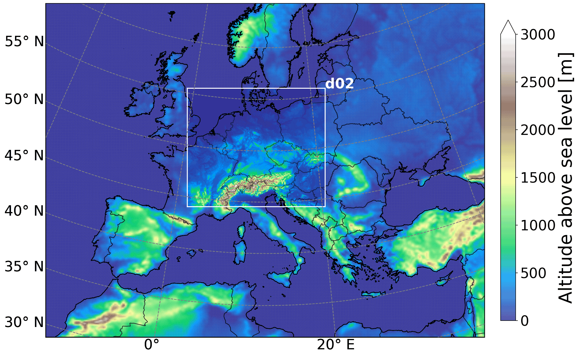
Figure B1 Nested model domains d01 (full figure) and d02 (marked panel) of the WRF simulations.

B1.2 DWD weather stations

Germany's National Meteorological Service (Deutscher Wetterdienst, DWD) provides hourly measurements of surface temperature, pressure, and relative humidity for a network of ground stations in Germany (Kaspar et al., 2013). Data are provided via the climate data center web interface (CDC-v2.1; https://cdc.dwd.de/portal/, last access: 18 May 2021). The meteorological measurements are performed in accordance to the guidelines of the WMO to minimize local effects. Additionally, we have applied quality control filters such that the QUALITAETS_BYTE (QB) is below 4 (thereby excluding untested, objected, and calculated values), and QUALITAETS_NIVEAU (QN) is either 3 (automatic control and correction) or 7 (second control done, before correction) to only retain measurements of high quality. By applying these criteria, we retained 98.2 %, 100 %, and 99.5 % of T₀, p₀, and RH₀ data, respectively. Note that using only data with QN =10 (the best possible quality check level) would result in no data left for the period considered in this study. If only QN =7 had been applied, we would have retained the same number of T₀ and RH₀ but no p₀ data.

For this study, we extract DWD measurements for May to June 2018, 06:00 to 17:00 UTC, and only consider stations providing T₀, p₀, and RH₀ simultaneously, resulting in 206 stations which are displayed in Fig. B2.

Figure B2 Location of the 206 DWD ground stations providing simultaneous measurements of surface values of T, p, and RH during May to June 2018.

B1.3 Validation of WRF surface values

We use the DWD network of surface stations for investigating the accuracy and precision of the WRF simulations. Figure B3 displays correlations between surface values from the DWD station network and the respective WRF simulations. For this purpose, each station is associated with the nearest neighbor from the WRF simulation. We do not interpolate the WRF data as we still want to compare the parameterized O₄ VCD with the true VCD derived from vertical integration of the WRF profiles.

Surface altitude (a) is lower in the gridded elevation map used as input in the WRF simulations by 20 m on average, and by almost 1 km for the station on Germany's highest mountain, Zugspitze. This is a consequence of the spatial resolution of the WRF simulations of 1 km, which is not sufficient for resolving single mountains. The systematic negative bias of WRF surface altitude indicates that the DWD stations tend to be located on hill and mountain tops.

This difference in altitude would directly affect the comparisons of T and particularly p. Thus, we apply a simple correction of station values and extrapolate them to the respective WRF surface altitude assuming a lapse rate of −6.5 K km⁻¹. For RH, no correction is applied.

The comparison reveals a good agreement between surface values from WRF and DWD, with remaining systematic biases of WRF simulations of −1 K for T₀ and 1 % for RH₀.

Table B1 List of GRUAN stations and number of available sonde flights (only considering $\text{SZA}<\mathrm{85}{}^{\circ }$) used in this study.

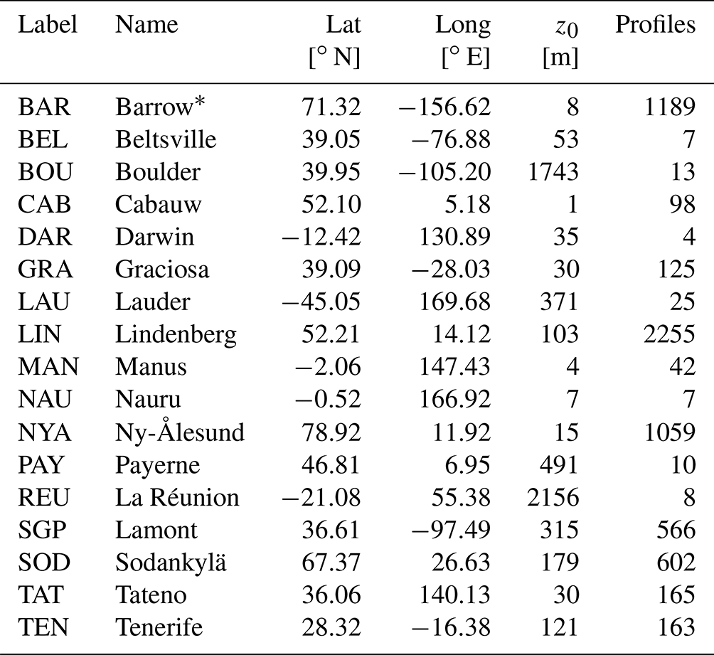
^* now Utqiaġvik.

B2 GRUAN stations

The GRUAN stations used in this study are listed in Table B1, including station shortcut and full name, latitude, longitude, altitude of the station, and the number of available profiles with $\text{SZA}<\mathrm{85}{}^{\circ }$. Figure B4 displays a map showing the GRUAN station locations.

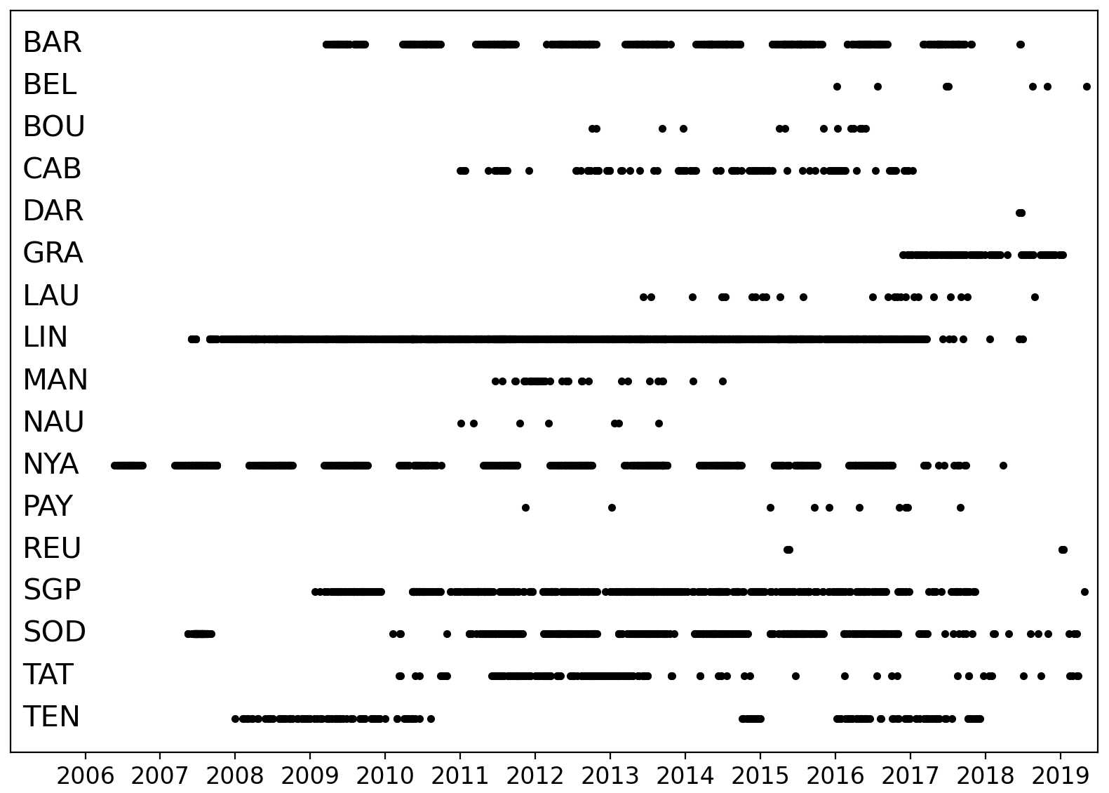
The temporal cover of radio sonde measurements at the different stations is displayed in Fig. B5. Note that some stations only contribute a low number of measurements. Still, we decided to keep all stations, as the application of a threshold for a minimum number of profiles of, e.g., 50 would remove all tropical sites (Darwin, Manus, and Nauru).

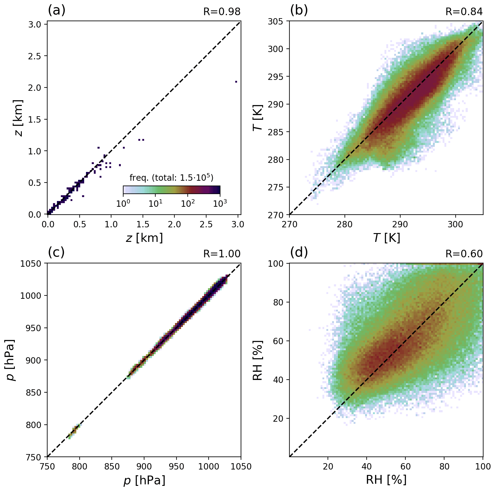
Figure B3 Comparison of WRF surface values (y axis) to DWD ground stations (x axis). For T and p, station values are adjusted to the mean altitude of the respective gridded elevation map used as input for WRF simulations (see text for details).

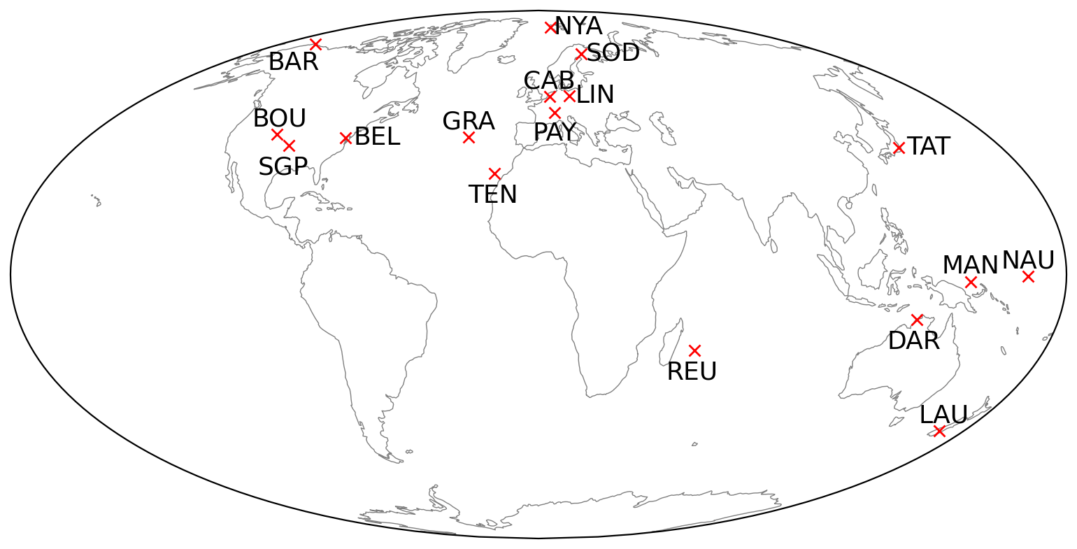
Figure B4 Location of GRUAN stations considered in this study. For station names and further details see Table B1.

Figure B5 Time of the available sonde flights (with $\text{SZA}<\mathrm{85}{}^{\circ }$) for the GRUAN stations considered in this study. For station names and further details see Table B1.

Appendix C: Additional ERA5 results

Figures C1 and C2 display additional results for δ_Γ and δ_RH, respectively, for 18 March and 18 September 2018.

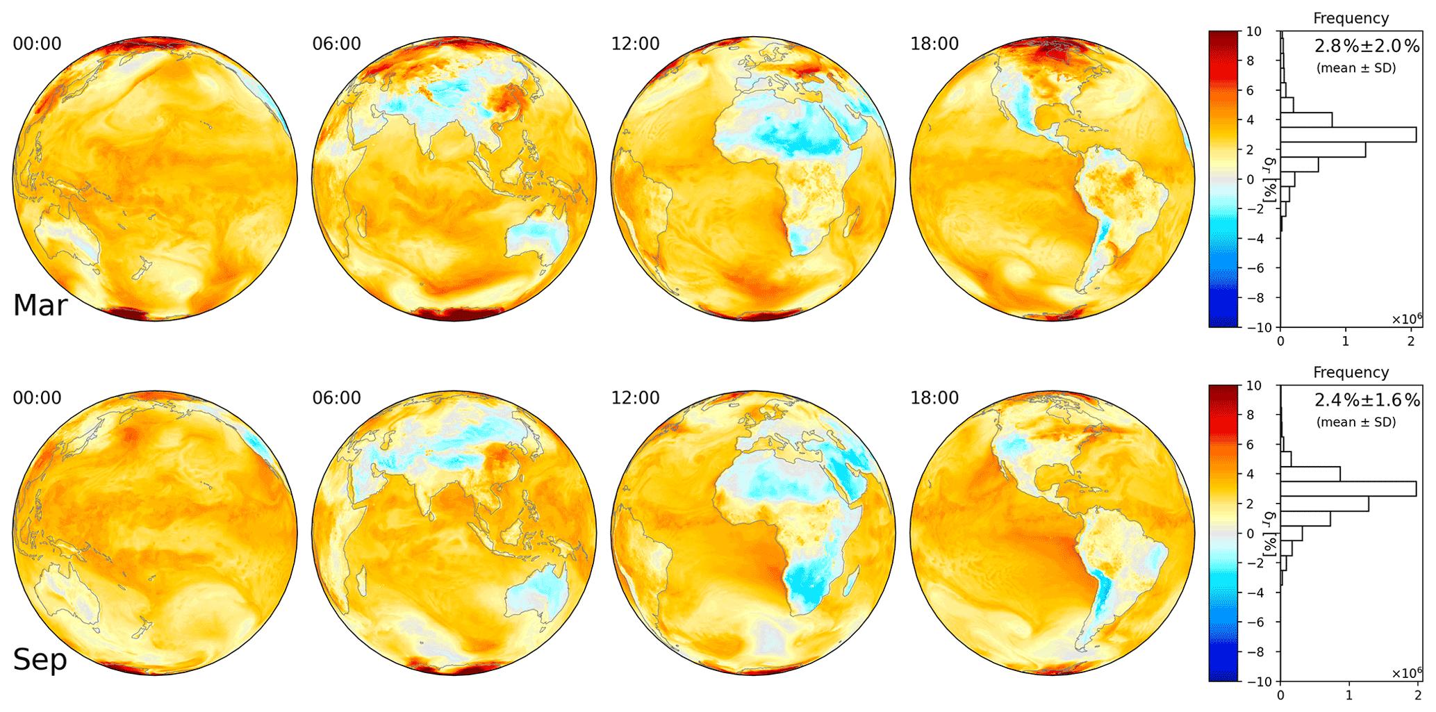
Figure C1 Deviation δ_Γ according to Eq. (19) for ERA5 at 00:00, 06:00, 12:00, and 18:00 UTC on 18 March (top) and 18 September (bottom) 2018. The projection focuses on daytime for each time step. On the right, the frequency distribution and mean and SD are given for all hourly outputs of the respective day.

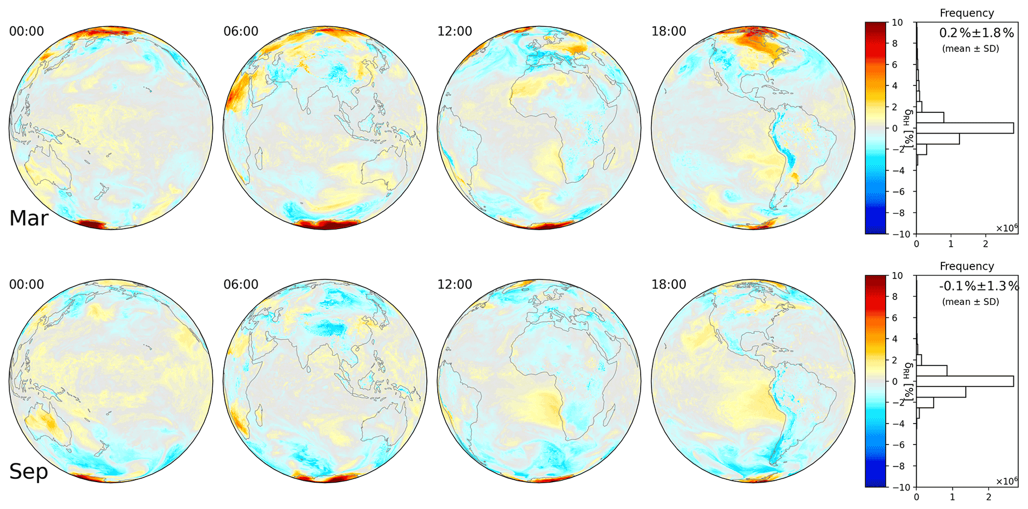
Figure C2 Deviation δ_RH according to Eq. (19) for ERA5 at 00:00, 06:00, 12:00, and 18:00 UTC on 18 March (top) and 18 September (bottom) 2018. The projection focuses on daytime for each time step. On the right, the frequency distribution and mean and SD are given for all hourly outputs of the respective day.