the Creative Commons Attribution 4.0 License.
the Creative Commons Attribution 4.0 License.
 | 03 Mar 2023
Relationship between the sub-micron fraction (SMF) and fine-mode fraction (FMF) in the context of AERONET retrievals
Norman T. O'Neill
Keyvan Ranjbar
Liviu Ivănescu
Thomas F. Eck
Jeffrey S. Reid
David M. Giles
Daniel Pérez-Ramírez
Jai Prakash Chaubey
The sub-micron (SM) aerosol optical depth (AOD) is an optical separation based on the fraction of particles below a specified cutoff radius of the particle size distribution (PSD) at a given particle radius. It is fundamentally different from spectrally separated FM (fine-mode) AOD. We present a simple (AOD-normalized) SM fraction versus FM fraction (SMF vs. FMF) linear equation that explains the well-recognized empirical result of SMF generally being greater than the FMF. The AERONET inversion (AERinv) products (combined inputs of spectral AOD and sky radiance) and the spectral deconvolution algorithm (SDA) products (input of AOD spectra) enable, respectively, an empirical SMF vs. FMF comparison at similar (columnar) remote sensing scales across a variety of aerosol types.
SMF (AERinv-derived) vs. FMF (SDA-derived) behavior is primarily dependent on the relative truncated portion (εc) of the coarse-mode (CM) AOD associated with the cutoff portion of the CM PSD and, to a second order, the cutoff FM PSD and FM AOD (εf). The SMF vs. FMF equation largely explains the SMF vs. FMF behavior of the AERinv vs. SDA products as a function of PSD cutoff radius (“inflection point”) across an ensemble of AERONET sites and aerosol types (urban-industrial, biomass burning, dust, maritime and a mixed class of Arctic aerosols). The overarching dynamic was that the linear SMF vs. FMF relation pivots clockwise about the approximate (SMF, FMF) singularity of (1, 1) in a “linearly inverse” fashion (slope and intercept of approximately 1−εc and εc) with increasing cutoff radius. SMF vs. FMF slopes and intercepts derived from AERinv and SDA retrievals confirmed the general domination of εc over εf in controlling that dynamic. A more general conclusion is the apparent confirmation that the optical impact of truncating modal (whole) PSD features can be detected by an SMF vs. FMF analysis.
- Article
(4381 KB) - Full-text XML
-
Supplement
(697 KB) - BibTeX
- EndNote


Anderson et al. (2005) noted the “decades-old observation that aerosol mass generally consists of two modes: (1) a mechanically produced coarse mode (CM) and (2) a fine mode (FM) produced by combustion and/or gas-to-particle conversion”. Typical CM examples include wind-eroded desert dust and sea salt, while FM aerosols tend to be dominated by biomass-burning smoke and anthropogenic and biogenic (ABF) fine particles (the latter classification being proposed, for example, by Lynch et al., 2016). Given this speciated physical reality (and notwithstanding the known chemical and microphysical internally mixed changes that occur in aerosol properties as they are transported through the atmosphere), there is a certain level of justification in treating different species of aerosols as independent FM and CM particle size distributions (PSDs). The degree of rigor in this modal paradigm is, in fact, the subject of model analyses that compare prescribed bulk aerosol PSDs with sectional (binned) PSDs (see, for example, Mann et al., 2012, for the case of size-referenced PSDs and Kodros and Pierce, 2017, for the case of mass-referenced PSDs).
AERONET inversions (AERinv), derived from input spectral AODs and solar almucantar radiances (Dubovik and King, 2000), provide a comprehensive suite of microphysical and optical products (at approximately hourly temporal resolutions). The general tendency towards (particle-volume) PSD bimodality is notably evidenced in retrieved AERinv PSDs (see, for example, Fig. 1 of Dubovik et al., 2002; Fig. 11a of Eck et al., 2009; and Fig. 3 of AboEl-Fetouh et al., 2020).1 A bimodal optical representation of that PSD bimodality (without the requirement of having to specify the PSD shape of each mode) can largely determine the measurable (low spectral order) optical behavior of remote sensing data (O'Neill et al., 2001, and references cited therein). O'Neill et al. (2003) employed spectral AODs (sampling intervals ∼ 3 min) as an input to their spectral deconvolution algorithm (SDA) to separate aerosols into (a) extensive (quantity dependent) FM and CM AOD components (τf and τc) of the total AOD (τa), (b) intensive (quantity-independent) spectral derivatives of τf (αf, , , etc.) and τc (αc, , , etc.) as components of the total AOD spectral derivatives (α, α′, α′′, etc.) and (c) semi-intensive FM and CM fractions (FMF and CMF represented, respectively, by and ). If aerosols can be viewed as independent coarse and fine modal features, then this purely spectral technique acts to separate those modal features in an optical sense.
The SMF (sub-micron fraction) is a microphysically determined alternative to the optically determined FMF: the division into fine and coarse components is effected by an explicit separation of the PSD at a cutoff radius (r0) that typically ranges from ∼ 0.4 to 1.1 µm across different types of aerosol volume sampling instruments.2 SMF separation represents a moderate but significant difference relative to the optically based FMF separation. Anderson et al. (2005) describe the SMF as “an operational definition … to distinguish it from the theoretical concept of fine-mode fraction, FMF”. Because the AERinv algorithm incorporates a cutoff radius division of the retrieved PSD into sub- and super-micron parameters (Dubovik and King, 2000), it is actually an SMF approach. Comparisons with the AERONET SDA product provide a unique opportunity to empirically analyze the SMF vs. FMF approaches at similar remote sensing (columnar) scales and across a global variety of aerosol types.
The literature on the direct comparison of the SMF vs. FMF retrievals is sparse and oftentimes at the margins of significance. The significance problem relates to the fact that one may be forced to extract relatively subtle microphysical and optical changes in the face of SMF and FMF variations that are often limited in range (lack of extensive-parameter aerosol variation and/or types for example). The sparsity of SMF vs. FMF investigations relates to limitations such as the rarity of experiments designed for such a comparison or the sparsity of data sets whose modes can be readily separated (by source information and/or chemical identification for example).
In the most controlled experiments, volume-sampled SMF estimates are compared with FMF retrievals derived from applying the SDA to volume-sampled, three-channel CRD (cavity ring-down) or three-channel nephelometer “spectra” (Atkinson et al., 2010; Kaku et al., 2014 (Ka); Atkinson et al., 2018). In general we find, as expected, the SMF to be ≳ FMF in Atkinson et al. (2010) and Ka: this is notably true at the near-IR (700 nm) wavelength in Ka (ACE-Asia data of their Fig. 2).3 The cases where this is not true (the T1 “ext_sum” results of Atkinson et al., 2018) are likely attributable to the spectral sensitivity of the FMF: this is most severe in the case of just three channels (for example, Ka's VOCALS 5% calibration correction of one 450 nm nephelometer channel transformed a case of SMF being substantially < FMF to a corrected case of SMF ∼ FMF).
Lesser constrained experiments involve multi-altitude, volume-sampled SMF estimates (from nephelometer scattering coefficient and absorption coefficient devices) compared with layer and column SDA-derived FMF estimates from multi-altitude AOD and ΔAOD spectra acquired with an airborne sun photometer (for example, Gassó and O'Neill, 2006, and Shinozuka et al., 2011, respectively, represented by the acronyms GO and SHN). In these cases, the lesser degree of experimental control (associated with multi-altitude flights) was somewhat offset by a more generous number of sun photometer spectral bands (four bands from the UV to the NIR in the GO case and five bands near the five bands employed in the AERONET SDA in the SHN case). The GO results were fairly coherent with SMF/FMF expectations (especially when the layered estimates were added to obtain columnar estimates) and quite marginal for SHN with a large spread of near-unity points about the SMF = FMF line (a situation with practically no significant SMF or FMF range and hence little relevant testing of their relationship). Analyses of the FMF vs. SMF relationship comparing satellite estimates of FMF4 with, for example, airborne estimates of SMF (Anderson et al., 2005) or coastal/island AERinv estimates of SMF (Kleidman et al., 2005) have proven difficult given the spectrally sensitive nature of the few bands employed in satellite-derived estimates of FMF and all the possible sources of incoherencies between the satellite retrievals and the ground-based or airborne estimates of SMF (differences in spatiotemporal sampling volumes for example).
A simple (approximate) relationship between the SMF and FMF will be presented below. We seek to demonstrate that the AERinv-derived value of SMF and the SDA-derived value of FMF are largely linked by that simple relationship and that fitting parameters extracted from their empirical comparison yield insight into their fundamental optophysical dynamics. We argue that the similar columnar scales as well as the diversity of AERONET aerosol types shared by the two retrievals facilitates the analysis of their second-order intensive-parameter relationship. It is emphasized that the AERinv and SDA algorithms were developed independently and share no explicit algorithmic links: what they do share is that the four spectral-AOD inputs to the AERinv represent four of the five spectral AODs employed as input to the SDA. What they do not share is the almucantar (angularly variable) radiance input employed in the AERinv retrieval. It is notable that the AERONET AOD is accurately measured with an estimated uncertainty of ∼ 0.01 and 0.02 in the visible/NIR and the UV, respectively (Eck et al., 1999), for an overhead sun (solar air mass of M = 1). This data quality enables both algorithms to, for example, retrieve notably consistent intensive parameter information such as particle size. The consistency is also attributable to the AERinv requirement that the retrieved AODs be within 0.01 of the measured AODs, while the second-order spectral fit to the AODs employed in the SDA has similar constraints (see, for example, Fig. 4 of O'Neill et al., 2001).
2.1 Size-cutoff integration versus modal integration
Figure 1 (generated from a simple lognormal fit to a sample AERinv particle-volume PSD retrieval5) illustrates the theoretical mechanical/optical framework of this paper. That fit was applied to lend an air of empirical relevance to this theoretical section: the discussion presented here is otherwise of a general nature and is not intended to represent an algorithmic step of the AERinv retrievals (or of the SDA for that matter). The FM and CM PSDs are represented by the red and blue lognormal curves, respectively. The SMF-type cutoff radius of r0 is represented by the black dashed vertical line where the associated optical and microphysical bimodal quantities are computed from both FM and CM PSDs to obtain sub-micron parameters to the left of r0 and super-micron parameters to the right of r0. The rest of the parameters in Fig. 1 are defined immediately below as we develop the theoretical framework.
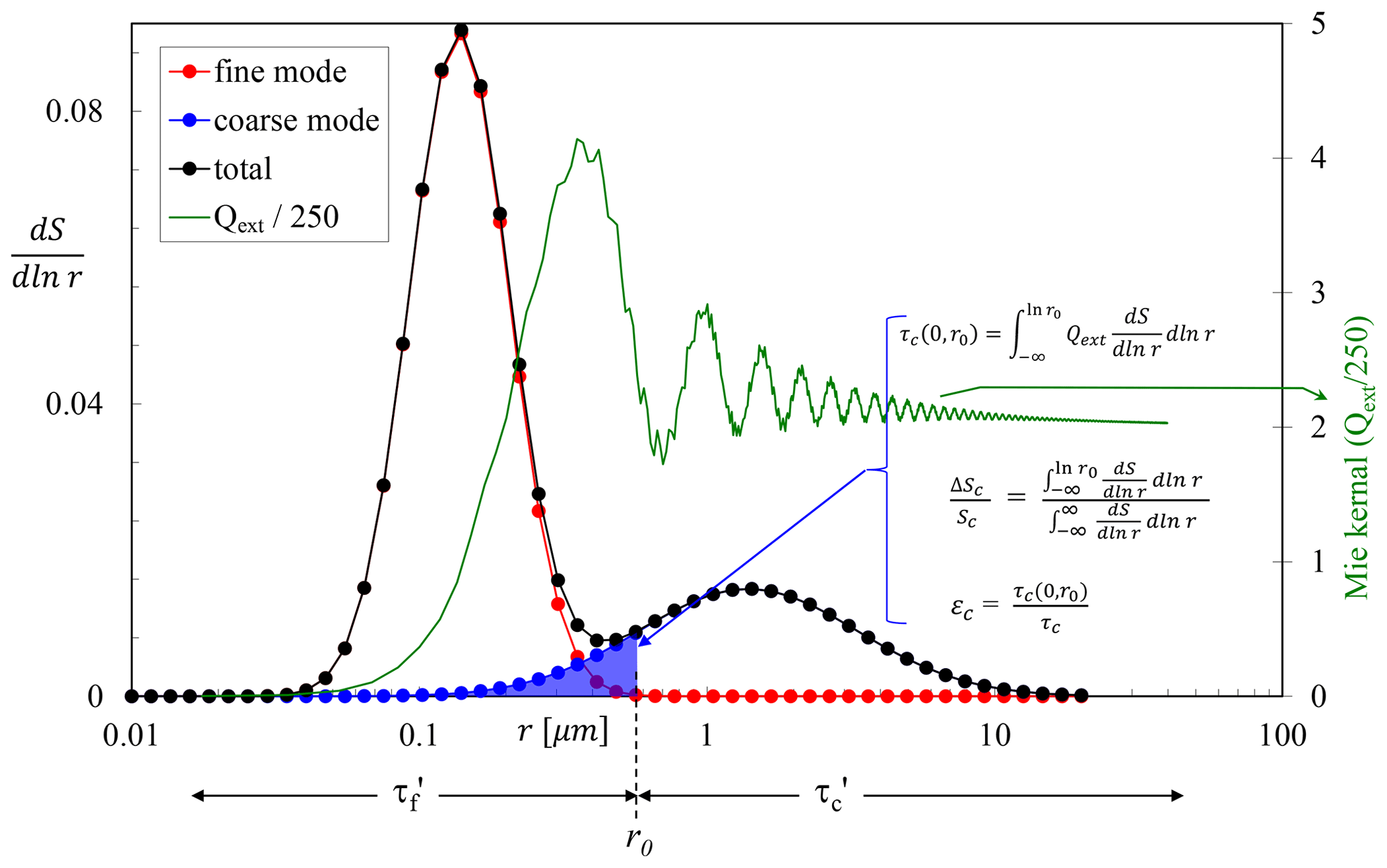
Figure 1Illustrative fine- and coarse-mode (red and blue) lognormal particle-surface size distributions () and the Mie kernel (extinction efficiency Qext) for a wavelength of 0.5 µm and a refractive index of 1.44−0.0035i (by particle-surface we mean the projected particle surface area of πr2). The cutoff radius (“inflection point” as it is called in the AERONET documentation) (r0) applies to an SMF type of computation. The total (black curve) is (in order to have a level of grounding in reality) the sum of the FM and CM lognormal curves that were individually manipulated to fit the mean of a series of AERONET and ground-based () FM and CM sea-salt curves reported in Fig. 8f of Reid et al. (2006). We base this illustration on as it is more optically fundamental than the AERinv particle-volume PSD (the projected particle surface area is employed to normalize the extinction cross section to obtain the fundamental extinction efficiency). An analogous explanation (and a graph similar to that of Fig. 2) would apply to the particle-volume PSD.
Letting prime variables refer to integrations which are carried out over size regimes of (0,r0) and (r0,∞) and unprimed variables refer to integrations carried out over entire modal features (over the entire FM or the entire CM PSDs), we can write the total AOD (τa) at some given reference wavelength as the sum of the fine and coarse total-modal AODs:
where (letting τx(r1, r2) refer to the optical integration from r1 to r2)
The analogous relationships in the domain of the cutoff size regimes are written as
with an emphasis on the “conservation of τa” (). The differences in the FM and CM (cutoff vs. modal) integrations are, respectively,
from which
The last expression is nothing more than confirmation of the “conservation of τa”.
2.2 SMF versus FMF
Using the definitions and relationships given above, we can now define FMF and SMF, respectively, as
and
Given that , we divide by τa to obtain
and with a little manipulation,
where εf and εc represent the pure truncation errors of the FM and CM PSDs (the second terms of Eq. 5a and 5b normalized by τa):
and
These two quantities represent intensive parameter (largely quantity independent)6 attributes. Typically however, εc≫εf (the major part of the FM PSD is well displaced to the left of r0 as per the illustration of Fig. 1). This has much more of a cutoff impact on the blue-colored CM PSD of Fig. 1 than on the red-colored FM PSD: the solid blue cutoff portion (ΔSc) is a significant portion of the CM particle-surface density (Sc), and τc(0,r0) is a significant optical depth portion of τc (i.e., both and εc are typically significant), while the analogous FM fractions above r0 are relatively insignificant. This affirmation, which we will empirically demonstrate in the multi-station analysis below, is, in part, related to the fact that the FM PSD is approximately half the width of the CM PSD (Dubovik et al., 2002; in their paper “width” specifically refers to the σ value of fitted lognormal distributions).
Table 1Site coordinates, predominant aerosol type, sampling periods and retrieval numbers for the AERONET inversions and SDA retrievals employed in this study.

a N = the number of retrievals. See the Methodology section of the text for details on how the AERONET inversion and SDA retrievals were matched. b Goddard Space Flight Center. c Polar Environment Arctic Research Lab. The acronym represents the total atmospheric research infrastructure at Eureka, Nunavut, Canada. The AERONET/AEROCAN site is more accurately referred to as the PEARL Ridge Lab. d Barrow Atmospheric Baseline Observatory.
Figure 2 is a plot of εc vs. for a variety of retrievals from the sites listed in Table 1. All these cases involved, as per the Fig. 1 illustration, the fitting of FM and CM lognormal curves to AERinv particle-volume PSDs (and a subsequent transformation to particle-surface parameters). These lognormal fits permit the explicit (Mie-based) calculations of the Eq. (7b) fractions. They represent a (AERONET-grounded) theoretical illustration of an expected strong correlation between cutoff optics and cutoff mechanics (the correlation is less than monotonic because of variations in refractive index and the width of the lognormal curves for the different cases chosen in this illustration). We emphasize that automated lognormal fits to AERinv PSDs are not part of the empirical analyses presented in this paper (nor do they have any role in the purely spectral SDA retrieval); rather, the purpose of Fig. 2 is to confirm the expected strong correlation between optical and microphysical CM cutoff fractions and thereby facilitate an understanding of εc's role in the dynamics of Eq. (7a).
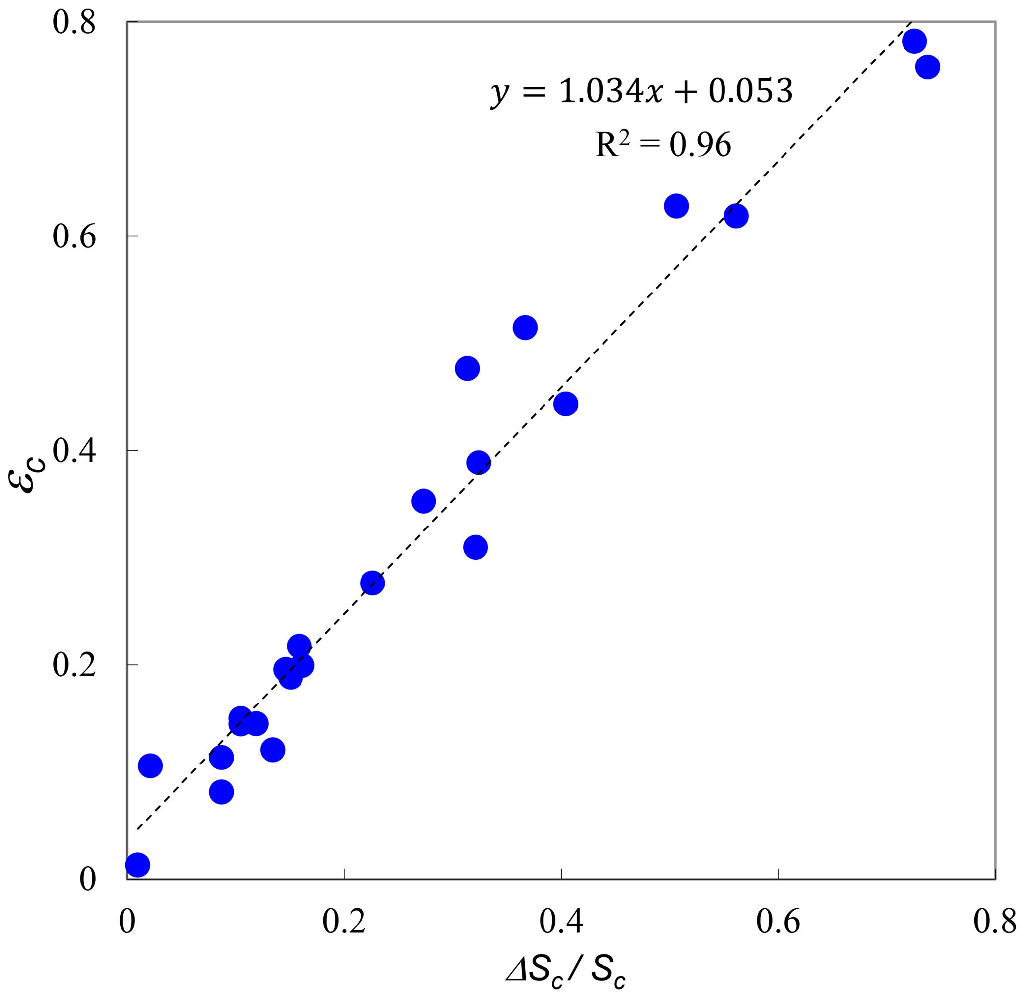
Figure 2Plot of εc vs. for a variety of simulated optical depth retrievals. The lognormal FM and CM PSDs employed in these simulations were obtained by fitting their sum to retrieved AERinv PSDs over a variety of sites whose predominant aerosol type was urban, dust or marine (and employing the refractive indices provided by the retrieval product). The AERinv PSD retrievals were Version 2, for which r0 was fixed at 0.6 µm and, accordingly, for which the εc vs. regression would be only dependent on εc and second-order parameters such as refractive index (i.e., the plot is independent of r0).
The linear form of Eq. (7a) with its sub-unity slope of and positive εc intercept is coherent with empirical results of η′ being generally ≳ η (the well-recognized empirical result, supported by the results presented below, of SMF being generally ≳ FMF). Because εc generally dominates εf, the linear η′ vs. η relation pivots clockwise about the point in a “linearly inverse” fashion (slope and intercept of approximately 1−εc and εc). Figure 3 shows a set of Eq. (7a) straight lines for representative ranges of different εc and εf values that were inspired by the ranges encountered in the empirical results that follow.
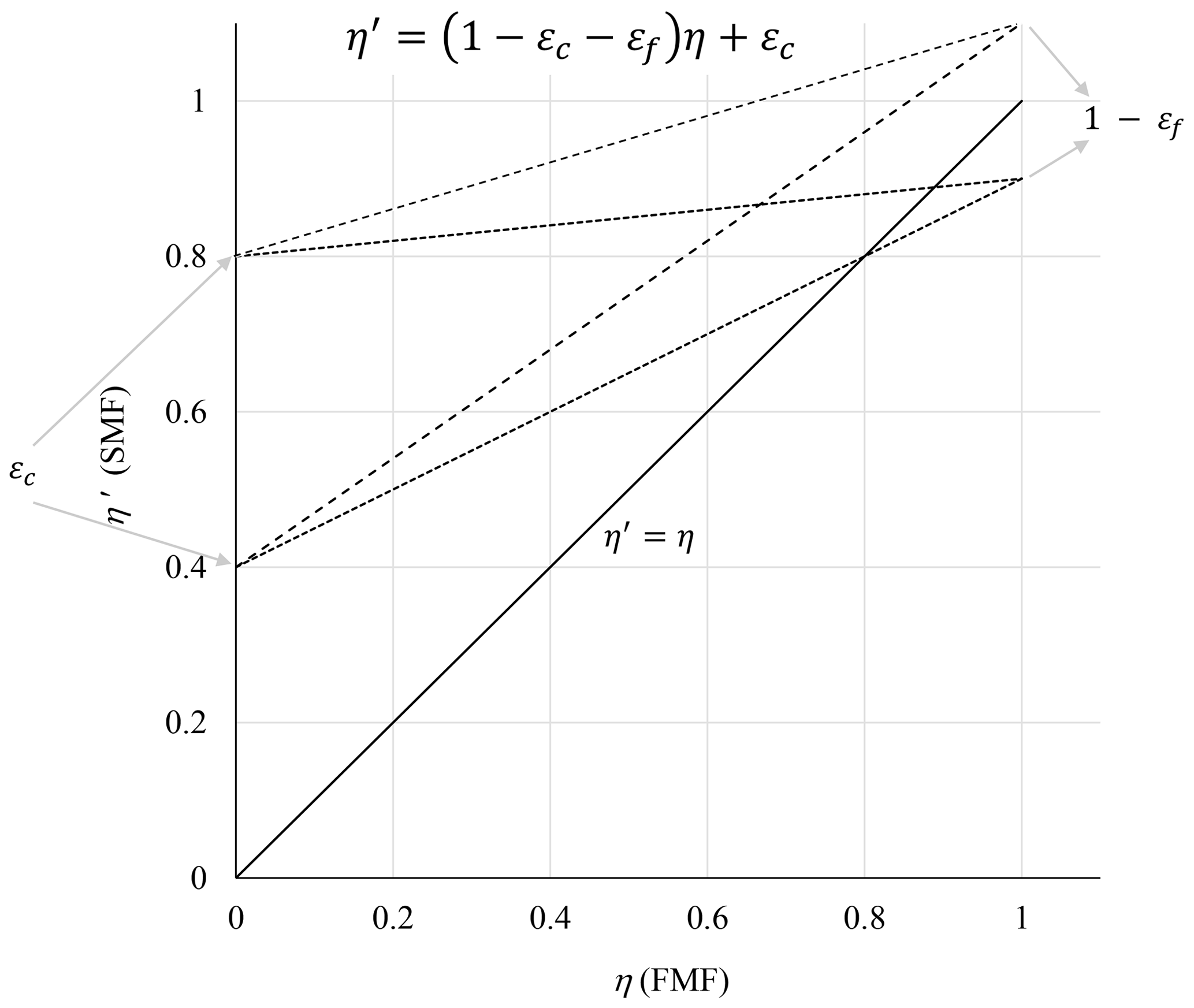
Figure 3η′ (SMF) vs. η (FMF) lines of Eq. (7a) for three εc values and three εf values (0, 0.4 and 0.8 and −0.1, 0 and 0.1, respectively). The εc values were inspired by the range of empirical values seen in Fig. 6 (and, in the case of εf, by the range of values, whether real or artifactual, seen in Fig. 7).
Cases of large εf are relatively rare but would occur during intense FM events characterized by large-amplitude FM PSDs that are shifted towards larger radii: illustrations include strong (large FM AOD) smoke events (see, for example, the sub-Arctic (Alaskan) smoke cases of AOD(440 nm) ≳ 1 in Fig. 9a of Eck et al., 2009) and strong FM pollution events enhanced by high relative humidity (see, for example, the PSDs corresponding to AOD(440 nm) ≳ 2 in Fig. 4 of Eck et al., 2020). However an increasing εf presupposes that r0 is fixed (as for volumetric surface sampling devices): the AERinv technique of setting the r0 value to the minimum of the PSD (see below) results in a minimization of εf.
Hesaraki et al. (2017) give an overview of the AERinv and SDA with an emphasis on the fact that the former is a significantly more comprehensive algorithm whose low frequency sampling rate is appropriate for detailed climatological-scale analyses (see, for example, Dubovik et al., 2002; AboEl-Fetouh et al., 2020), while the high frequency sampling rate of the SDA is better suited to the detailed analysis of diurnal events (see, for example, Fig. S5 of Saha et al., 2010). The SDA is readily applied to AOD spectra generated by star photometers and moon photometers (see, for example, Baibakov et al., 2015), while analogous AERinv products (requiring an almucantar scan) do not exist for nighttime conditions.
In this investigation, we “matched” SDA to AERinv retrievals by employing averages of Version 3 Level 2.0 AODs (Giles et al., 2019) as inputs to the SDA if those AODs were within a time window of ±16 min about the nominal AERinv times.7 Version 3 AERinv products (Sinyuk et al., 2020) were employed to derive estimates of SMF, and . The cutoff radius for those products is actually defined as the minimum of the AERinv output particle-volume PSD () with a restriction that the radius bin centers of that minimum must be one of four AERinv bins (r0, which is referred to as an “inflection point” in AERONET documentation is allocated a AERinv bin-center value of 0.439, 0.576, 0.756 or 0.992 µm). The AERinv retrievals of and are interpolated to the SDA reference wavelength of 500 nm using a second-order (log–log space) spectral polynomial regressed to the and values at the four AERinv wavelengths of 440, 675, 870 and 1020 nm (the same technique employed in the SDA).

Figure 4AERONET stations employed for generating the statistics employed in this paper. These stations were chosen to represent a regional variety of aerosols (pollution, biomass burning, dust mixtures, sea-salt mixtures and Arctic aerosols). See Table 1 for details.
A variety of AERONET sites (Fig. 4), representing different types (classes) of aerosols, were chosen to investigate the SMF versus FMF relationship. These aerosol classes (Table 1) included sites known for FM urban-industrial aerosols (GSFC in Greenbelt, MD, USA), FM biomass burning (Mongu, Zambia), CM dust (Crete, Hamim and Solar Village), CM maritime aerosols (Midway Island and Lanai), a mixture of dust and marine aerosols (FORTH, Crete) and a mixture of high-Arctic aerosols (PEARL and Thule) as well as low-Arctic aerosols (Barrow Atmospheric Baseline Observatory, referred to as Barrow hereafter). Our choice of aerosol types was not intended to be comprehensive from the standpoint of investigating variations in, say, different types of smoke aerosols or different types of dust aerosols; rather, we sought to properly exercise the SMF versus FMF relationship by largely filling the admissible portion of the SMF versus FMF scattergram (see Fig. 3).
The Arctic category is a mixed class of aerosols: its inclusion in our table of aerosol types is more in terms of it representing an important comparative test (relative to the applicability of southern latitude findings) in a region where the aerosol signal is notably weak. Arctic illustrations of FMF vs. SMF principles feature more in the analysis presented below precisely because the signal is weak: the observation of an independently verified FMF vs. SMF trend or characteristic in the Arctic is an indicator of the robustness of that observation. This weak-signal robustness is something we often see for Arctic retrievals (see, for example, the FM and CM results of AboEl-Fetouh et al., 2020): it may well be (at least in part) attributable to the large solar zenith angles (large solar air mass, M) and attendant decrease in optical depth errors (a typical finding over 20 years of AERONET Mauna Loa calibrations according to co-author Thomas F. Eck; see also Fig. 2 of Karanikolas et al. (2022) for an empirical validation of this error dependency).
4.1 Frequency of occurrence of inflection (r0) points
Figure 5 shows the relative frequency of occurrence (FO) of the four different AERinv inflection (r0) points for the different Table 1 classes. The relative importance of CM PSDs vs. FM PSDs for the dust class sites of Solar Village and Hamim and the marine sites of Midway Island and Lanai push the AERinv minimum to smaller r0 values (resulting in an FO dominance at the 0.439 µm inflection point). The marine sites are moderately less asymmetric (less pushed towards 0.439 µm) than the dust sites, because the CM PSDs for the dust sites tend to be of larger amplitude. There are, however, other factors at play that could have some impact on the FO distributions; for example, large FM sulfatic particles from Kīlauea eruptions that might push back on the CM PSD dominance of marine particles at Lanai and/or non-sphericity effects of dust that, when corrected (Dubovik et al., 2006), would produce a significantly larger FM PSD amplitude (a complication that does not impact the predominantly spherical marine particles).
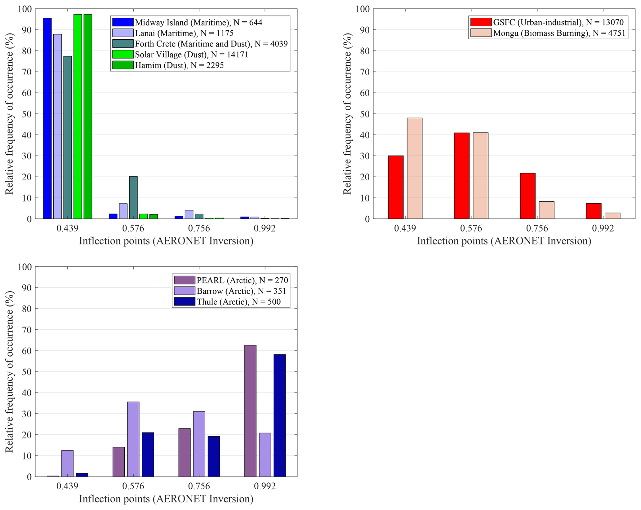
Figure 5Relative frequency occurrence (FO) distributions for the four different AERONET inflection points (r0 values with units of µm) for all Table 1 AERONET sites.
The two sites that are heavily influenced by strong FM PSDs (the Mongu biomass-burning site and the GSFC urban-industrial site) tend (as suggested above in an εf context) to “push” the PSD minimum towards larger r0 values relative to the dust and marine sites (resulting in a more balanced FO curve in Fig. 5). Eck et al. (2001) attributed this FM particle-size increase to coagulative effects for Mongu (see their Fig. 6), while Eck et al. (2012) attributed the increase to the effects of hygroscopically induced FM particle growth at the GSFC site (see their Fig. 17). Other smoke-impacted and urban-industrial sites show similar coagulative particle growth effects (see Fig. 10b of Eck et al., 2019, for specific cases recorded in the Southeast Asian tropical forest) and hygroscopic particle growth impacts (see, for example, Fig. 13 of Eck et al., 2005, for Beijing). We argue below that these large-amplitude increases in FM particle size are, given the AERinv technique of variable inflection points, relatively minor in terms of producing significant εf values.
The Arctic sites show a FM PSD domination which produces an FO distribution that is not unlike the Mongu distribution in the singular case of Barrow, while being much more skewed towards large r0 for PEARL and Thule. We illustrate below (as part of a discussion on the variation of εc) that a systematic (seasonal) spring-to-summer inflection point increase can be attributed to the Arctic sites.
4.2 η′ vs. η (SMF vs. FMF) scattergrams
Figure 6 shows η′ vs. η (SMF vs. FMF) scattegrams representing four key aerosol types of Table 1 (scattergrams for the rest of the aerosol types and sites can be seen in Fig. S1 of the Supplement). The theoretical solid black lines of Fig. 6 represent various values of εc in Eq. (7a); we chose to set εf to zero in tracing those lines because its value is, as indicated above, generally small (and to not obscure the graphs with second-order detail). We note (as per the previous discussion of the FO distributions) that as the AERinv PSD minimum radius (inflection point) increases, the cutoff portion of the CM PSD increases (resulting in the transition from red to blue curves). The slopes tend to decrease (swing clockwise) with an attendant increase in the intercepts.
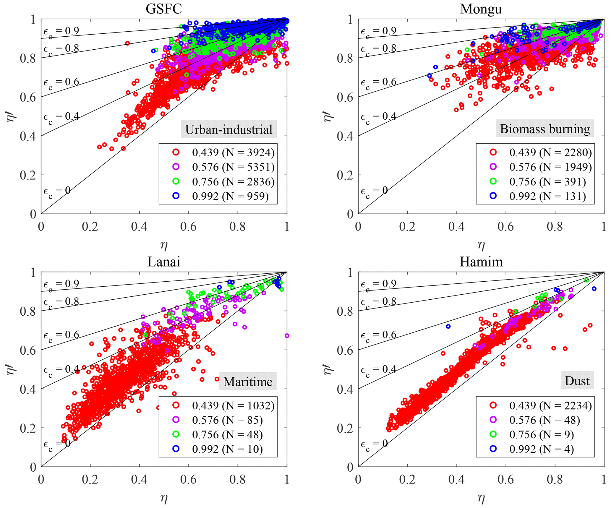
Figure 6η′ vs. η (AERinv-derived SMF vs. SDA-derived FMF) scattergrams for the sites of GSFC, Mongu, Lanai and Hamim (aerosol types of urban-industrial, biomass burning, marine and dust, respectively, as per Table 1). The four colors represent the four different AERinv inflection points (r0 values with units of µm). The remaining scattergrams for the other sites are shown in Fig. S1. The solid black lines are those of Eq. (7a), with εf set to zero (for the sake of the simplicity of the presentation coupled with the fact that εf plays a relatively minor role).
The FO dominance of the 0.439 µm r0 bin is most evident for the CM-dominated dust class (Hamim) with, practically speaking, a single (small εc) red-colored grouping of points being observable, while the more balanced distributions of FO curves for GSFC and Mongu provide four clear point groupings. In the extreme of CM cutoff, virtually all of the optically significant contributions of the CM PSD are eliminated, and an asymptote of with εc→1 for all values of η is approached (the slope of Eq. 7a approaches zero). That extreme CM cutoff condition is most evident for the blue, large-r0 points of the GSFC scattergram), where a regression slope could be almost parallel to the η′ axis. We did indeed find r0=0.992 cases associated with near-unity η′ values for which most of the optically significant portion of the CM PSD was cut off, while the FM and CM PSDs were not inordinately unbalanced in terms of amplitude (η was some sub-unity value of significance for which there were no apparent problems associated with the AOD spectra).
The small to large r0 (red to blue) transformation translates, for example, into a classical seasonal pattern for the Arctic scattergrams of Fig. S1; the springtime amplitude of the small-sized CM PSD (that AboEl-Fetouh et al., 2020, associated with Asian dust) decreases progressively from spring to summer. This weakening of CM influence induces a spring-to-summer increase in the value of r0 and, by extension, εc (see the seasonal r0 histograms and derived table for Barrow in Fig. S2). This is an effect that is more noticeable in the Level-1.5 AERinv products of AboEl-Fetouh et al. (2020) than the Level-2 products of this paper.8
Within the theoretical context of Eq. (7a), the scattergrams of Fig. 6 show (predominantly for the red-colored 0.439 µm inflection value of r0), a minority of unphysical points below the line (points for which ). An investigation into the most extreme cases of this inequality indicated that the wayward points were more inclined to be associated with abnormally large values of η (rather than abnormally small values of η′) and small AODs (≲ 0.05). Figure 10 of O'Neill et al. (2003) shows the noise sensitivity of η values to such small AODs if one assumes an rms AOD error of 0.01 in all bands (0.01 being ≲ errors of AERONET field instruments). In general, this type of small-AOD sensitivity was reported empirically by, for example, Fig. 7 of Eck et al. (1999) and Figs. 8 and 9 of O'Neill et al. (2001). The fundamental dynamic is that a band-to-band AOD discontinuity ≲ 0.01 can generate important perturbations in small-AOD curvature spectra and produce significant outliers in the spectrally sensitive η values.
4.3 Analysis of the slopes and intercepts (derivation of εc and εf)
The η′ vs. η scattergrams support the hypothesis that there is a physical/optical interpretation that can be given to the slope and intercept of Eq. (7a) (that Eq. 7a and 7b are theoretically relevant approximations). Figure 7a and b show the regression slopes vs. the intercepts derived for, respectively, all sites and all r0 values of the Fig. 6 and Supplement scattergrams,9 while Table 2 lists the associated regression statistics for the 0.439 µm inflection point. The large range of the intercept seen in Fig. 7 confirms that the cutoff portion of the CM PSD (εc of Eq. 7b) is much more determinant in affecting the interplay of η′ vs. η. The position of the colored circles relative to the dashed or dotted black lines (derived from Eq. 7a and 7b) visually support the Table 2 results of small εf (εf values being ≲ 0.07 according to their positions between the εf=0 and εf=0.1 grid lines).
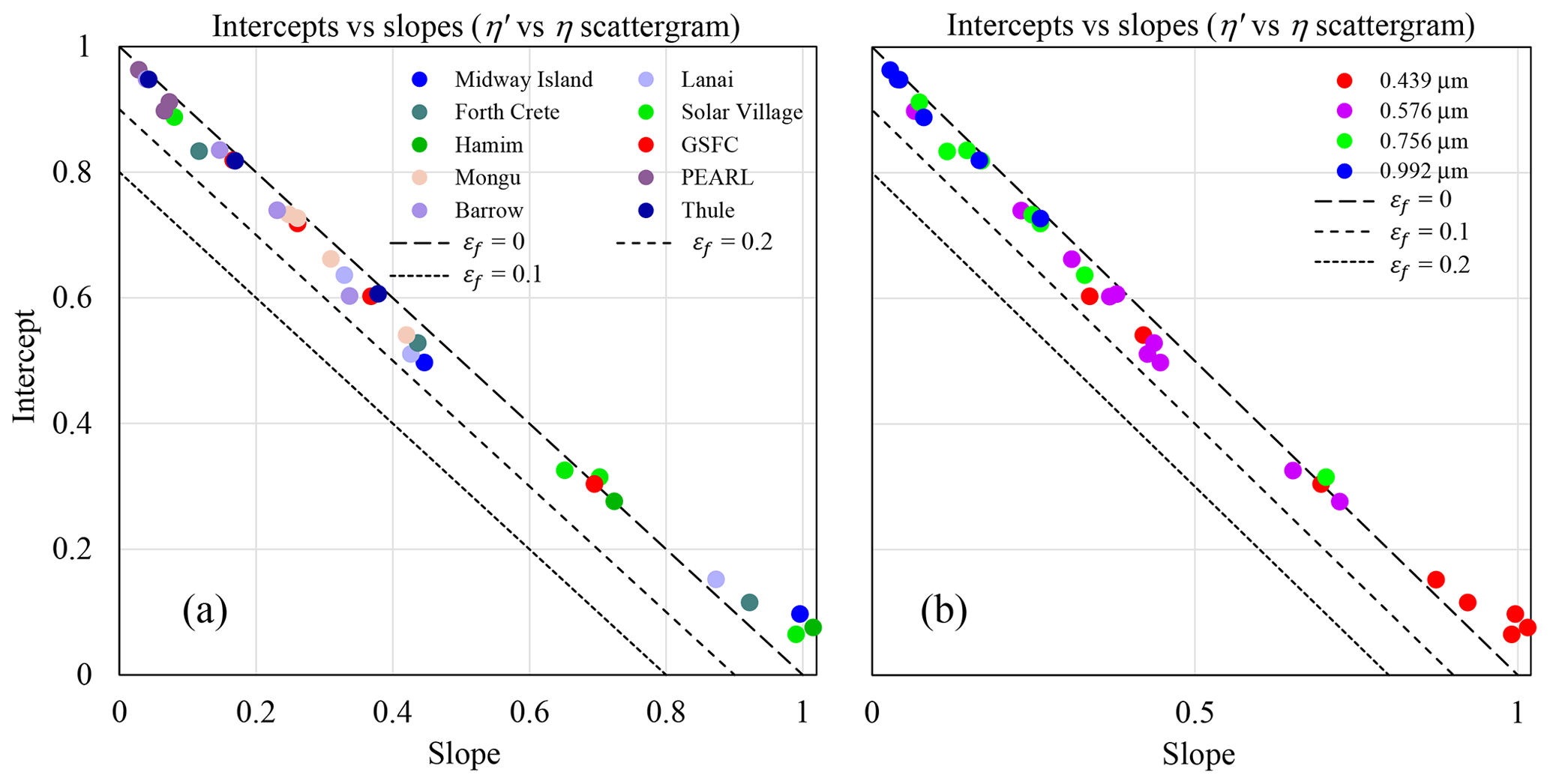
Figure 7Intercept vs. slope plots for the η′ vs. η scattergrams as a function of (a) all the sites of Table 1 and (b) the cutoff r0 value (AERinv inflection point radius). The black dashed or pointed lines represent the family of straight lines generated by Eq. (7a): slope = and intercept = εc for values of εc=0 to 1 and three values of εf (0.0, 0.1 and 0.2).
Table 2η' vs. η regression stats for r0=0.439 µma.
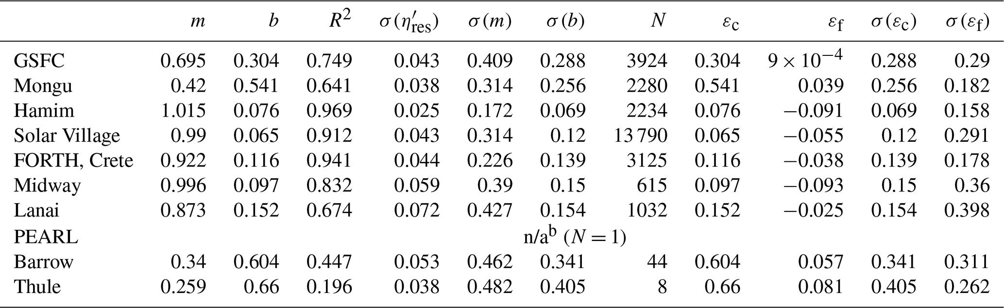
a See, for example, Taylor (1997) for typical regression relationships. The εc and εf values as well as their standard deviation (σεc) and σ(εf) were derived from the regressed slope and intercept (“m” and “b”) using the slope and intercept expressions of Eq. (7a). The values of (σ(εc) and σ(εf)) are computed from effective standard deviations of m and b. By this, we mean that the standard error (from sources such as Taylor, 1997) is multiplied by to yield σ(m) and σ(b): this transforms the unrealistically small m and b uncertainties into values that are more representative of the variation seen in the scattergrams of Fig. 6. This change is coherent with the notion that those variations are more likely due to εc and εf being characterized by a systematic range of values for any given inflection point (r0) value. Note that represents the standard deviation of the regression residuals.
b n/a: not applicable.
The values corresponding to the five red-colored (0.439 µm inflection point) circles for the desert and marine sites (bottom right-hand corner of Fig. 7b) are, however, outside the physically coherent range of Eq. (7). The negative values of εf (see Table 2) can be inferred from the εf=0, 0.1, 0.2 grid of Fig. 7b or, more visually, from the unphysical (super-unity) slopes that arise from a regression through the red points of the desert and marine scattergrams of Fig. 6. This incoherency is very likely the result of those regression lines representing a non-unique ensemble of εc and εf values. From an optophysical standpoint, they vary as a function of the diversity of dust and marine CM PSDs that are predominantly associated with the 0.439 µm inflection point (they roughly lie between the εc=0 and εc=0.4 boundaries of Fig. 3; the η=1 intercept10 will (in consequence of a super-unity slope) yield negative values above the intercept).
Non-systematic noise will also impact the derived εc and εf values. Scattergrams of vs. τf for the two sites that are largely dominated by strong FM variations (GSFC and Mongu) and which showed the most balanced (Fig. 5) FO distributions are shown in Fig. A1. One can observe, in the first instance, the point-dispersion reduction and the convergence towards the line as both increase (as τa increases). The extensive (quantity-dependent) nature of those scattergrams complements the analogous η′ vs. η semi-intensive scattergrams of Fig. 6 by explicitly displaying the noise-like influences of the amount of aerosol ( or τf) as well as r0. The vs. τf dispersion of Fig. A1 is nonetheless generally small; this underscores a hypothesis that the η′ vs. η results presented above are robust second-order findings. The FO distributions of η′ vs. η in Fig. A2 effectively eliminate the extensive variations of Fig. A1 with an attendant enhancement of those second-order influences.
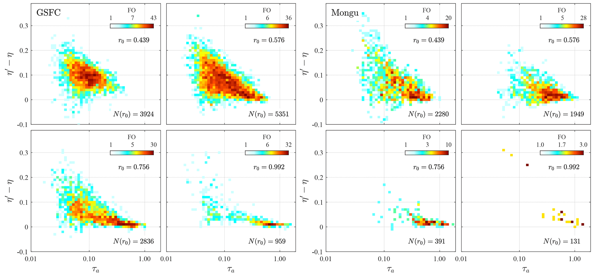
The Fig. 8 FO distributions of vs. τa more readily show the decreasing dispersion and the convergence towards the () line with increasing τa (increasing τf values for GSFC and Mongu). The broad left-to-right movement of the (red) FO peak values with increasing r0 (notably in the case of GSFC) also clarifies an aspect that is not easily discernable in the highly correlated scattergrams of Fig. A1: that an increase in r0 is coarsely associated with η′ values that approach η or, hence, values that approach τf (a trend that effectively drives the () convergence induced by increasing τa).
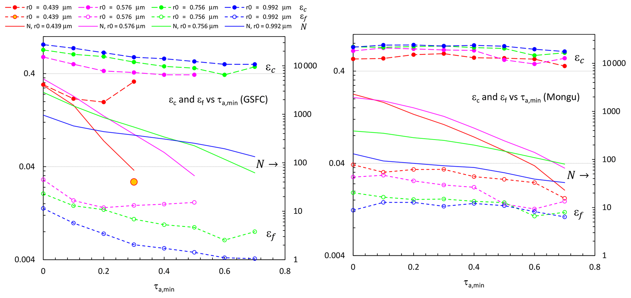
Figure 9GSFC and Mongu variations of regression-derived values of εc and εf as a function of a minimum value of total AOD at 500 nm (τa, min) employed in the η′ vs. η regressions (The decreasing point dispersion (the approach of to τf) with increasing τf indicates that the regression-derived precision of the εc and εf values should, for that reason alone, generally increase with larger values of τf. However, offsetting this type of influence on an increase in precision is the decrease in the number of regression points and the squeeze in τf and variability as the singularity is approached.) (to be clear, Fig. 9 represents an exercise in testing the sensitivity to τa, min: the regressions of Fig. 6 and the regression-derived εc and εf values of Fig. 7 were obtained with no restrictions on the matched AERinv and SDA retrievals). Same color scheme as Figs. 6 and 7. The legend of the Mongu plot is the same as the GSFC legend. The number of matched retrievals (N) is also shown (right-hand axis). Result are not shown in cases where N<20. The large orange-filled (re-rimmed) circle in the GSFC case represents the only εf point of the r0=0.439 µm regressions that both survived the N<20 rejection criterion and did not yield a negative εf value.
Figure 9 shows the regression-derived εc and εf variation as a function of an artificial minimum (τa, min) in the lower bound of the τa regression range (see the Fig. 9 caption for more details). The result shows no strong εc dependency on τa, min and more variable but consistently small amplitudes of εf.11 Qualitatively, these observations are not unexpected given the fairly persistent slope of the high FO (red-colored ellipses of Fig. A2).
The choice of a variable r0 in the AERinv retrievals clearly means that the affirmation of increasing εf in the presence of strong FM events (i.e., what would be measured by a traditional fixed-r0 device) cannot readily be observed with the AERinv retrievals. Strong FM events basically push the FM PSD to larger radii (while the CM PSD remains relatively inactive12). The AERinv approach of selecting r0 as the minimum of the PSD basically neuters the cutoff of significant optical portions of the FM PSD. The general tendency for r0 to increase with increasing τf in Fig. 8 is consistent with the concept of the FM PSD being pushed to the right as and τf increase.
AERinv PSDs can differ from the simple bimodal paradigm incorporated in Eqs. (1) through (7). The bimodality of the Arctic CM PSDs of AboEl-Fetouh et al. (2020) were ascribed to a small-sized CM feature in the 1.3 µm AERinv bin (a systematic feature that they attributed to Asian dust) and a larger-sized mode that might have been linked to local dust and/or sea salt. Eck et al. (2012) reported a bimodal FM PSD (their Fig. 3) that they attributed to cloud processing of FM pollution (haze) aerosols. In such cases, one can appeal to the optical equivalency of, for example, a bimodal CM PSD to a single CM PSD whose curvature parameters become averages of those of the two CM components (see Appendix A for the two specific cases of a bimodal CM PSD with a unimodal FM PSD as well as a bimodal FM PSD with a unimodal CM PSD). This means that the bimodal expressions of O'Neill et al. (2001) still apply for the AERONET SDA product and thus that the FMF to SMF expressions (Eqs. 1 to 7) can still be used.
The FMF (SDA) approach is arguably the more fundamental approach for separating FM and CM optical contributions, because it is intrinsically related to the modal nature of different types of aerosols (at least to the first order: modality becomes obscured, for example, with internal mixing of different aerosol types). The SMF (AERinv) approach is the more pragmatic approach, as it is commonly and readily applied to microphysical surface and airborne measurements. It is however, as we have seen in results like those of Fig. 6, very dependent on the selected cutoff radius.
We presented a simple SMF vs. FMF (η′ vs. η) equation that enabled an understanding of the well-recognized empirical result of SMF being larger than the FMF. This result has been reported for in situ, satellite and ground-based remote sensing techniques; our focus was on an SMF vs. FMF interpretation in the form of AERinv SMF vs. SDA FMF retrievals. We pointed out that these two AERONET products provide a unique opportunity to empirically compare the SMF and FMF approaches at similar (columnar) remote sensing scales and across a shared global variety of aerosol types.
The SMF vs. FMF equation largely captured the SMF vs. FMF behavior of the AERinv vs. SDA products as a function of inflection point (r0) across an ensemble of AERONET sites and aerosol types (urban-industrial, biomass burning, dust, marine, maritime and Arctic). The SMF vs. FMF behavior was primarily dependent on the intensive parameter of relative cutoff portion of the CM PSD (εc) and, to a second order, the relative cutoff portion of the FM PSD (εf). The overarching dynamic was that the linear SMF vs. FMF relation pivots clockwise about the point in a “linearly inverse” fashion (slope and intercept of approximately 1−εc and εc) with increasing r0. Derived SMF vs. FMF slopes and intercepts confirmed the general domination of εc over εf in controlling the “linear inverse” variation. The process of deriving and analyzing εc and εf values demonstrated an expected domination of FM optical depths for the urban pollution and biomass-burning sites of GSFC and Mongu and thus a convergence towards the ( line as τa increased (the convergence of SDA FM AODs towards AERinv FM AODs).
The more general conclusion resulting from this analysis is the apparent empirical confirmation that the influence of PSD modal features can be detected by an indirect comparative analysis. While one would like to believe that this is true in general, a more comprehensive event-level closure experiment employing, for example, multi-altitude microphysical and optical measurements over a representative suite of AERONET instruments would do much to increase the level of confidence in such a conclusion.
A1 Frequency of occurrence analyses
The retrieval results in this subsection are restricted to the two sites that are strongly impacted by historically large variations in FM particles (GSFC and Mongu). These sites (details in Table 1) can experience τf values greater than unity.

Figure A1 vs. τf frequency of occurrence (FO) distributions for GSFC and Mongu. The FO color scale is tied to variations on a logarithmic scale (with an attendant tendency to enhance the contributions of large FO values). N(r0) is the total FO at a given r0 value.
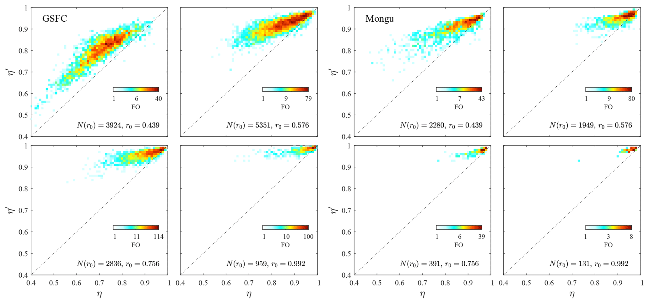
Figure A2η′ vs. η FO distributions for GSFC and Mongu. See the caption of Fig. A1 for FO and N(r0) details.
A2 Dual-modal optical equivalency of a trimodal size distribution
A2.1 Fine mode and two coarse modes
One often sees a bimodal coarse-mode PSD and thus a trimodal PSD. Treating the bimodal CM PSD as an optically equivalent single-mode CM PSD can be formalized as below (optical equivalent of Eq. 1a of O'Neill et al., 2003):
where , and . Accordingly,
Equation (3) of O'Neill et al. (2003) can be written as
where represents the optical average of αc1 and αc2. Equation (A3) is exactly the analog of O'Neill et al. (2003). Differentiating and recalling that , one finds that
but since , we can replace (α−αf) and (α−〈αc〉) to obtain
so that
These expressions are optically equivalent to Eq. (5) of O'Neill et al. (2003) with their Eq. (5) values being transformed according to
where the average value of any parameter xc is always
A2.2 Coarse mode and two fine modes
In this instance one can imagine two fine-mode components; for example, (i) large-sized FM smoke and (ii) smaller sized FM urban-industrial pollution. The algebra above for the single FM PSD and two CM PSDs can be employed here: everything is perfectly reversible (interchange index c with index f) if η is viewed as the ratio of coarse to total AOD. Then arriving at the final equations for α and α′, one can return to the usual definition of η to obtain the same algebraic theorem. The classic equations for α and α′ remain unchanged providing one employs the substitutions below:
where , and . Explicitly,
| AEROCAN | Federated Canadian subnetwork of AERONET run by Environment and Climate Change Canada (ECCC) |
| AERONET | AErosol RObotic NETwork: worldwide NASA network of combined sun photometer/sky-scanning radiometers manufactured by CIMEL Éléctronique. See http://aeronet.gsfc.nasa.gov/ (last access: 25 February 2023) for documentation and data downloads. |
| AOD | Aerosol optical depth: the community uses “AOD” to represent anything from nominal aerosol optical depth which has not been cloud-screened to the conceptual (theoretical) interpretation of aerosol optical depth. In this paper we use it in the latter sense and apply adjectives as required. |
| AERinv | AERONET inversion |
| SDA | Spectral deconvolution algorithm |
| CM | Coarse mode |
| εc | Relative truncation error of the CM PSD (Eq. 7b) |
| εf | Relative truncation error of the FM PSD (Eq. 7b) |
| η | FMF (product of the SDA) |
| η′ | SMF (product of the AERinv) |
| FM | Fine mode |
| FO | Frequency of occurrence |
| PSD | Particle size distribution (notably the AERinv particle-volume size distribution, , in the context of this paper) |
| FMF | Fine-mode fraction (an output parameter computed from SDA products) |
| SMF | Sub-micron fraction (an output parameter computed from AERinv products) |
| r0 | Cutoff radius (units of µm) that separates the PSD into FM and CM components. The AERONET parameter name is “inflection point” (but it would be more pragmatically labelled as the PSD minimum; the bin-center location of the minimum of the retrieved PSD). |
| τa | Total aerosol optical depth at 500 nm (SDA) |
| τc | Coarse-mode aerosol optical depth at 500 nm (SDA) |
| τf | Fine-mode aerosol optical depth at 500 nm (SDA) |
| Total aerosol optical depth at 500 nm | |
| Coarse-mode aerosol optical depth at 500 nm using a cutoff radius of r0 (derived AERinv product) | |
| Fine-mode aerosol optical depth at 500 nm using a cutoff radius of r0 (derived AERinv product) |
All AERinv and SDA retrieval data are available from the AERONET website (https://doi.org/10.17616/R3VK9T, Lind and Gupta, 2023).
The supplement related to this article is available online at: https://doi.org/10.5194/amt-16-1103-2023-supplement.
NTO'N led the conceptualization, methodology and formal analysis. All co-authors contributed to the revisions of the manuscript. TFE, JSR and DMG provided fundamental comments that resulted in substantial changes to the manuscript. KR, LI, DPR and JPC were instrumental in the strategical planning and operational processing of the data and the definition of the figures.
At least one of the (co-)authors is a member of the editorial board of Atmospheric Measurement Techniques.
Publisher’s note: Copernicus Publications remains neutral with regard to jurisdictional claims in published maps and institutional affiliations.
We acknowledge the generous permission of the principal investigators of the 10 AERONET sites used in this study for the use of their AERinv and SDA retrieval data. The principal investigators are the following: Brent Holben of AERONET/NASA (Goddard Space Flight Center) at the Hamim, GSFC, Lanai, Midway Island, Solar Village, Thule and Mongu sites, Ihab Abboud and Vitali Fioletov of AEROCAN/Environment and Climate Change Canada (ECCC) at the PEARL site, Richard Wagener of Brookhaven National Laboratory (BNL) at the Barrow site and Andrew Clive Banks of Hellenic Centre for Marine Research (HCMR) for the FORTH, Crete, site.
This work was supported by the GSFC/NASA AERONET project (led by Brent Holben), CANDAC (the Canadian Network for the Detection of Atmospheric Change) through the PAHA (Probing the Atmosphere of the High Arctic) project led by James Drummond of CANDAC, the NSERC Discovery Grant program (Norman T. O'Neill), CSA's ESS-DA program (the SACIA-2 project led by Norman T. O'Neill) and CSA's FAST program (CASSAVA – PEARL project led by Kimberly Strong of CANDAC).
This research has been supported by the National Aeronautics and Space Administration, Goddard Space Flight Center (grant no. SURA-GSTR-4100-NASA), the Canadian Space Agency (grant nos. 500353/15FASTA12, 19ATORA07, 16SUASACIA and 21SUASACOA), and the Natural Sciences and Engineering Research Council of Canada (grant nos. CREATE 384996-10, RGPCC-433842-2012 and RGPIN-2017-05531).
This paper was edited by Linlu Mei and reviewed by three anonymous referees.
AboEl-Fetouh, Y., O'Neill, N. T., Ranjbar, K., Hesaraki, S., Abboud, I., Fioletov, V., and Sobolewski, P. S.: Climatological-scale analysis of intensive and semi-intensive aerosol parameters derived from AERONET Arctic retrievals, J. Geophys. Res.-Atmos., 125, e2019JD031569, https://doi.org/10.1029/2019JD031569, 2020.
Anderson, T. L., Wu, Y., Chu, D. A., Schmid, B., Redemann, J., and Dubovik, O.: Testing the MODIS satellite retrieval of aerosol fine-mode fraction, J. Geophys. Res.-Atmos., 110, D18204, https://doi.org/10.1029/2005JD005978, 2005.
Atkinson, D. B., Massoli, P., O'Neill, N. T., Quinn, P. K., Brooks, S. D., and Lefer, B.: Comparison of in situ and columnar aerosol spectral measurements during TexAQS-GoMACCS 2006: testing parameterizations for estimating aerosol fine mode properties, Atmos. Chem. Phys., 10, 51–61, https://doi.org/10.5194/acp-10-51-2010, 2010.
Atkinson, D. B., Pekour, M., Chand, D., Radney, J. G., Kolesar, K. R., Zhang, Q., Setyan, A., O'Neill, N. T., and Cappa, C. D.: Using spectral methods to obtain particle size information from optical data: applications to measurements from CARES 2010, Atmos. Chem. Phys., 18, 5499–5514, https://doi.org/10.5194/acp-18-5499-2018, 2018.
Baibakov, K., O'Neill, N. T., Ivanescu, L., Duck, T. J., Perro, C., Herber, A., Schulz, K.-H., and Schrems, O.: Synchronous polar winter starphotometry and lidar measurements at a High Arctic station, Atmos. Meas. Tech., 8, 3789–3809, https://doi.org/10.5194/amt-8-3789-2015, 2015.
Dubovik, O. and King, M. D.: A flexible inversion algorithm for retrieval of aerosol optical properties from Sun and sky radiance measurements, J. Geophys. Res., 105, 20673–20696, https://doi.org/10.1029/2000JD900282, 2000.
Dubovik, O., Holben, B. N., Eck, T. F., Smirnov, A., Kaufman, Y. J., King, M. D., Tanré, D., and Slutsker, I.: Variability of absorption and optical properties of key aerosol types observed in worldwide locations, J. Atmos. Sci., 59, 590–608, https://doi.org/10.1175/1520-0469(2002)059<0590:VOAAOP>2.0.CO;2, 2002.
Dubovik, O., Sinyuk, A., Lapyonok, T., Holben, B. N., Mishchenko, M., Yang, P., Eck, T. F., Volten, H., Muñoz, O., Veihelmann, B., Van der Zande, W. J., Leon, J.-F., Sorokin, M., and Slutsker, I.: Application of spheroid models to account for aerosol particle nonsphericity in remote sensing of desert dust, J. Geophys. Res.-Atmos., 111, D11208, https://doi.org/10.1029/2005JD006619, 2006.
Eck, T. F., Holben, B. N., Reid, J. S., Dubovik, O., Smirnov, A., O'Neill, N. T., Slutsker, I., and Kinne, S.: Wavelength dependence of the optical depth of biomass burning, urban, and desert dust aerosols, J. Geophys. Res.-Atmos., 104, 31333–31349, https://doi.org/10.1029/1999JD900923, 1999.
Eck, T. F., Holben, B. N., Ward, D. E., Dubovik, O., Reid, J. S., Smirnov, A., Mukelabai, M. M., Hsu, N. C., O'Neill, N. T., and Slutsker, I.: Characterization of the Optical Properties of Biomass Burning Aerosols in Zambia during the 1997 ZIBBEE experiment, J. Geophys. Res.-Atmos., 106, 3425–3448, https://doi.org/10.1029/2000JD900555, 2001.
Eck, T. F., Holben, B. N., Dubovik, O., Smirnov, A., Goloub, P., Chen, H. B., Chatenet, B., Gomes, L., Zhang, X.-Y., Tsay, S.-C., Ji, Q., Giles, D. M., and Slutsker, I.: Columnar aerosol optical properties at AERONET sites in central Eastern Asia and aerosol transport to the tropical Mid-Pacific, J. Geophys. Res.-Atmos., 110, D06202, https://doi.org/10.1029/2004JD005274, 2005.
Eck, T. F., Holben, B. N., Reid, J. S., Sinyuk, A., Dubovik, O., Smirnov, A., Giles, D. M., O'Neill, N. T., Tsay, S. C., Ji, Q., Al Mandoos, A., Ramzan Khan, M., Reid, E. A., Schafer, J. S., Sorokine, M., Newcomb, W. W., and Slutsker, I.: Spatial and temporal variability of column-integrated aerosol optical properties in the southern Arabian Gulf and United Arab Emirates in summer, J. Geophys. Res.-Atmos., 113, D01204, https://doi.org/10.1029/2007JD008944, 2008.
Eck, T. F., Holben, B. N., Reid, J. S., Sinyuk, A., Hyer, E. J., O'Neill, N. T., Shaw, G. E., Vande Castle, J. R., Chapin, F.S., Dubovik, O., Smirnov, A., Vermote, E., Schafer, J. S., Giles, D. M., Slutsker, I., Sorokine, M., and Newcomb, W. W.: Optical Properties of Boreal Region Biomass Burning Aerosols In Alaska and Transport of Smoke to Arctic Regions, J. Geophys. Res.-Atmos., 114, D11201, https://doi.org/10.1029/2008JD010870, 2009.
Eck, T. F., Holben, B. N., Reid, J. S., Giles, D. M., Rivas, M. A., Singh, R. P., Tripathi, S. N., Bruegge, C. J., Platnick, S., Arnold, G. T., Krotkov, N. A., Carn, S. A., Sinyuk, A., Dubovik, O., Arola, A., Schafer, J. S., Artaxo, P., Smirnov, A., Chen, H., and Goloub, P.: Fog- and cloud-induced aerosol modification observed by the Aerosol Robotic Network (AERONET), J. Geophys. Res.-Atmos., 117, D07206, https://doi.org/10.1029/2011JD016839, 2012.
Eck, T. F., Holben, B. N., Giles, D. M., Slutsker, I., Sinyuk, A., Schafer, J. S., Smirnov, A., Sorokin, M., Reid, J. S., Sayer, A. M., Hsu, N. C., Shi, Y. R., Levy, R. C., Lyapustin, A., Rahman, M. A., Liew, S.-C., Salinas Cortijo, S. V., Li, T., Kalbermatter, D., Keong, K. L., Yuggotomo, M. E., Aditya, F., Maznorizan M., Mastura M., Chong, T. K., Lim, H.-S., Choon, Y. E., Deranadyan, G., Kusumaningtyas, S. D. A., and Aldrian, E.: AERONET remotely sensed measurements and retrievals of biomass burning aerosol optical properties during the 2015 Indonesian burning season, J. Geophys. Res.-Atmos., 124, 4722–4740, https://doi.org/10.1029/2018JD030182, 2019.
Eck, T. F., Holben, B. N., Kim, J., Beyersdorf, A. J., Choi, M., Lee, S., Koo, J.-H., Giles, D. M., Schafer, J. S., Sinyuk, A., Peterson, D. A., Reid, J. S., Arola, A., Slutsker, I., Smirnov, A., Sorokin, M., Kraft, J., Crawford, J. H., Anderson, B. E., Thornhill, K. L., Diskin, G., Kim, S.-W., and Park, S.: Influence of cloud, fog, and high relative humidity during pollution transport events in South Korea: Aerosol properties and PM2.5 variability, Atmos. Environ., 232, 117530, https://doi.org/10.1016/j.atmosenv.2020.117530, 2020.
Gassó, S. and O'Neill, N. T.: Comparisons of remote sensing retrievals and in situ measurements of aerosol fine mode fraction during ACE-Asia, Geophys. Res. Lett., 33, L05807, https://doi.org/10.1029/2005GL024926, 2006.
Giles, D. M., Sinyuk, A., Sorokin, M. G., Schafer, J. S., Smirnov, A., Slutsker, I., Eck, T. F., Holben, B. N., Lewis, J. R., Campbell, J. R., Welton, E. J., Korkin, S. V., and Lyapustin, A. I.: Advancements in the Aerosol Robotic Network (AERONET) Version 3 database – automated near-real-time quality control algorithm with improved cloud screening for Sun photometer aerosol optical depth (AOD) measurements, Atmos. Meas. Tech., 12, 169–209, https://doi.org/10.5194/amt-12-169-2019, 2019.
Hamill, P., Giordano, M., Ward, C., Giles, D. M., and Holben, B. N.: An AERONET-based aerosol classification using the Mahalanobis distance, Atmos. Environ., 140, 213–233, https://doi.org/10.1016/j.atmosenv.2016.06.002, 2016.
Hesaraki, S., O'Neill, N. T., Lesins, G., Saha, A., Martin, R. V., Fioletov, V. E., Baibakov, K., and Abboud, I.: Polar summer comparisons of a chemical transport model with a 4-year analysis of fine and coarse mode aerosol optical depth retrievals over the Canadian Arctic, Atmos.-Ocean, 55, 213–229, https://doi.org/10.1080/07055900.2017.1356263, 2017.
Holben, B. N., Tanré, D., Smirnov, A., Eck, T. F., Slutsker, I., Abuhassan, N., Newcomb, W. W., Schafer, J. S., Chatenet, B., Lavenu, F., Kaufman, Y. J., Vande Castle, J., Setzer, A., Markham, B., Clark, D., Frouin, R., Halthore, R., Karneli, A., O'Neill, N. T., Pietras, C., Pinker, R. T., Voss, K., and Zibordi, G.: An emerging ground-based aerosol climatology: Aerosol optical depth from AERONET, J. Geophys. Res.-Atmos., 106, 12067–12097, https://doi.org/10.1029/2001JD900014, 2001.
Kaku, K. C., Reid, J. S., O'Neill, N. T., Quinn, P. K., Coffman, D. J., and Eck, T. F.: Verification and application of the extended spectral deconvolution algorithm (SDA+) methodology to estimate aerosol fine and coarse mode extinction coefficients in the marine boundary layer, Atmos. Meas. Tech., 7, 3399–3412, https://doi.org/10.5194/amt-7-3399-2014, 2014.
Karanikolas, A., Kouremeti, N., Gröbner, J., Egli, L., and Kazadzis, S.: Sensitivity of aerosol optical depth trends using long-term measurements of different sun photometers, Atmos. Meas. Tech., 15, 5667–5680, https://doi.org/10.5194/amt-15-5667-2022, 2022.
Kleidman, R. G., O'Neill, N. T., Remer, L. A., Kaufman, Y. J., Eck, T. F., Tanré, D., Dubovik, O., and Holben, B. N.: Comparison of Moderate Resolution Imaging Spectroradiometer (MODIS) and Aerosol Robotic Network (AERONET) remote-sensing retrievals of aerosol fine mode fraction over ocean, J. Geophys. Res.-Atmos., 110, D22205, https://doi.org/10.1029/2005JD005760, 2005.
Kodros, J. K. and Pierce J. R.: Important global and regional differences in aerosol cloud-albedo effect estimates between simulations with and without prognostic aerosol microphysics, J. Geophys. Res.-Atmos., 122, 4003–4018, https://doi.org/10.1002/2016JD025886, 2017.
Lind, E. and Gupta, P.: AERONET, Registry of Research Data Repositories re3data.org [data set], https://doi.org/10.17616/R3VK9T, 2023.
Lynch, P., Reid, J. S., Westphal, D. L., Zhang, J., Hogan, T. F., Hyer, E. J., Curtis, C. A., Hegg, D. A., Shi, Y., Campbell, J. R., Rubin, J. I., Sessions, W. R., Turk, F. J., and Walker, A. L.: An 11-year global gridded aerosol optical thickness reanalysis (v1.0) for atmospheric and climate sciences, Geosci. Model Dev., 9, 1489–1522, https://doi.org/10.5194/gmd-9-1489-2016, 2016.
Mann, G. W., Carslaw, K. S., Ridley, D. A., Spracklen, D. V., Pringle, K. J., Merikanto, J., Korhonen, H., Schwarz, J. P., Lee, L. A., Manktelow, P. T., Woodhouse, M. T., Schmidt, A., Breider, T. J., Emmerson, K. M., Reddington, C. L., Chipperfield, M. P., and Pickering, S. J.: Intercomparison of modal and sectional aerosol microphysics representations within the same 3-D global chemical transport model, Atmos. Chem. Phys., 12, 4449–4476, https://doi.org/10.5194/acp-12-4449-2012, 2012.
O'Neill, N. T., Eck, T. F., Holben, B. N., Smirnov, A., Dubovik, O., and Royer, A.: Bi-modal size distribution influences on the variation of Angstrom derivatives in spectral and optical depth space, J. Geophys. Res.-Atmos., 106, 9787–9806, https://doi.org/10.1029/2000JD900245, 2001.
O'Neill, N. T., Eck, T. F., Smirnov, A., Holben, B. N., and Thulesiraman, S.: Spectral discrimination of coarse and fine mode optical depth, J. Geophys. Res.-Atmos., 108, 4559, https://doi.org/10.1029/2002JD002975, 2003.
O'Neill, N. T., Thulasiraman, S., Eck, T. F., and Reid, J. S.: Robust optical features of fine mode size distributions: application to the Québec smoke event of 2002, J. Geophys. Res.-Atmos., 110, D11307, https://doi.org/10.1029/2004JD005157, 2005.
Ranjbar, K., O'Neill, N. T., Lutsch, E., McCullough, E. M., AboEl-Fetouh, Y., Xian, P., Strong, K., Fioletov, V. E., Lesins, G., and Abboud, I.: Extreme smoke event over the high Arctic, Atmos. Environ., 218, 117002, https://doi.org/10.1016/j.atmosenv.2019.117002, 2019.
Reid, J. S., Brooks, B., Crahan, K. K., Hegg, D. A., Eck, T. F., O'Neill, N. T., de Leeuw, G., Reid, E. A., and Anderson, K. A.: Reconciliation of coarse mode sea-salt aerosol particle size measurements and parameterizations at a subtropical ocean receptor site, J. Geophys. Res.-Atmos., 111, D02202, https://doi.org/10.1029/2005JD006200, 2006.
Saha, A., O'Neill, N. T., Eloranta, E., Stone, R. S., Eck, T. F., Zidane, S., Daou, D., Lupu, A., Lesins, G., Shiobara, M., and McArthur, L. J. B.: Pan-Arctic sunphotometry during the ARCTAS-A campaign of April 2008, Geophys. Res. Lett., 37, L05803, https://doi.org/10.1029/2009GL041375, 2010.
Shinozuka, Y., Redemann, J., Livingston, J. M., Russell, P. B., Clarke, A. D., Howell, S. G., Freitag, S., O'Neill, N. T., Reid, E. A., Johnson, R., Ramachandran, S., McNaughton, C. S., Kapustin, V. N., Brekhovskikh, V., Holben, B. N., and McArthur, L. J. B.: Airborne observation of aerosol optical depth during ARCTAS: vertical profiles, inter-comparison and fine-mode fraction, Atmos. Chem. Phys., 11, 3673–3688, https://doi.org/10.5194/acp-11-3673-2011, 2011.
Sinyuk, A., Holben, B. N., Eck, T. F., Giles, D. M., Slutsker, I., Korkin, S., Schafer, J. S., Smirnov, A., Sorokin, M., and Lyapustin, A.: The AERONET Version 3 aerosol retrieval algorithm, associated uncertainties and comparisons to Version 2, Atmos. Meas. Tech., 13, 3375–3411, https://doi.org/10.5194/amt-13-3375-2020, 2020.
Smirnov, A., Holben, B. N., Eck, T. F., Dubovik, O., and Slutsker, I.: Effect of wind speed on columnar aerosol optical properties at Midway Island, J. Geophys. Res.-Atmos., 108, 4802, https://doi.org/10.1029/2003JD003879, 2003.
Stone, R. S., Sharma, S., Herber, A., Eleftheriadis, K., and Nelson, D. W.: A characterization of Arctic aerosols on the basis of aerosol optical depth and black carbon measurements, Elem. Sci. Anth., 2, 000027, https://doi.org/10.12952/journal.elementa.000027, 2014.
Taylor, J. R.: An Introduction to Error Analysis: The Study of Uncertainties in Physical Measurements, 2nd edition, University Science Books, ISBN 9780935702750, 1997.
The examples in these papers can include the apparent presence of more than two modes (notably what often appear to be two CM sub-modes). Such cases are discussed below.
The expression “sub-micron” is generally “defocused” (relative to a literally exact value of 1.0 µm) to encompass this approximate range of r0 values. It is worth noting that the in situ community almost universally refers to diameter rather than radius.
For which the fixed cutoff radius for the optically smaller particles (and thus more optically active in the sense of more strongly attenuating) results in a greater relative contribution to the FM AOD (by “optically smaller”, we mean that the ratio of particle size to wavelength has decreased because the wavelength has increased). The optically smaller particles are more optically active as they are ascending the right side of the anomalous diffraction peak (see, for example, O'Neill et al., 2005).
These are retrievals that generally employ prescribed and speciated bulk (modal) FM and CM PSDs (of constant shape and position as a function of radius) as a basis for fitting spectral AODs at a few wavelengths.
The AERinv PSD particle-volume PSD () is readily transformed to the particle-surface PSD of Fig. 1 (). See the Fig. 1 caption for details.
By “largely quantity independent”, we mean, from an empirical standpoint, that τf(r0,∞) and τc(0,r0) are typically well correlated with τf and τc, respectively.
The number of AODs required to define a match in the time window could be as small as one (i.e., there was no minimum number).
The Level-2 processing tends to eliminate springtime retrievals completely: the majority of eliminations are due to excessive residuals in the retrieved vs. measured sky radiances that are, in turn, largely incited by the strong reflectance uncertainty of springtime snow (and its attendant impact on computed sky radiance) as well as the AERinv protocol of eliminating Level-2 retrievals if any snow is detected (by MODIS) within a 5 km radius of the site.
with a coherent color scheme between the scattergrams and Fig. 7b
for which
Except in the case of the (red) 0.439 µm r0 (yellow-filled) value where the εf variations were more substantial. At the same time, the number of regression points (N) rapidly decreases with increasing τa, min so that large εf (and εc) deviations are less statistically significant.
And it suffers from a per-particle extinction kernel (the green-colored Qext factor of Fig. 1) that is weaker in CM radius range.