A new algorithm to generate a priori trace gas profiles for the GGG2020 retrieval algorithm

Optimal estimation retrievals of trace gas total columns require prior vertical profiles of the gases retrieved to drive the forward model and ensure the retrieval problem is mathematically well posed. For well-mixed gases, it is possible to derive accurate prior profiles using an algorithm that accounts for general patterns of atmospheric transport coupled with measured time series of the gases in questions. Here we describe the algorithm used to generate the prior profiles for GGG2020, a new version of the GGG retrieval that is used to analyze spectra from solar-viewing Fourier transform spectrometers, including the Total Carbon Column Observing Network (TCCON). A particular focus of this work is improving the accuracy of CO₂, CH₄, N₂O, HF, and CO across the tropopause and into the lower stratosphere. We show that the revised priors agree well with independent in situ and space-based measurements and discuss the impact on the total column retrievals.

1 Introduction

The Total Carbon Column Observing Network (TCCON) has been in operation since 2004, beginning with its first dedicated instrument in Park Falls, WI, USA (Wunch et al., 2011). Since then, the network has expanded to 29 active sites located around the world. The network provides column average dry mole fractions (DMFs) of numerous gases, including carbon dioxide (CO₂), methane (CH₄), nitrous oxide (N₂O), hydrofluoric acid (HF), and carbon monoxide (CO). These observations have been used to infer or evaluate natural and anthropogenic carbon fluxes (e.g., Yang et al., 2007; Chevallier et al., 2011; Keppel-Aleks et al., 2012; Basu et al., 2013; Fraser et al., 2013; Ott et al., 2015; Peng et al., 2015; Deng et al., 2016; Wang et al., 2016; Feng et al., 2017; Hedelius et al., 2018; Crowell et al., 2019; Babenhauserheide et al., 2020; Dogniaux et al., 2021; Sussmann and Rettinger, 2020; Zhang et al., 2021; Villalobos et al., 2021), to study carbon transport (e.g., Keppel-Aleks et al., 2012; Polavarapu et al., 2016), and to provide ground truth values for space-based measurements of CO₂ and CH₄, including the Greenhouse gas Observing Satellites (GOSAT and GOSAT-2, e.g., Butz et al., 2011; Cogan et al., 2012; Schepers et al., 2012; Boesch et al., 2013; Frankenberg et al., 2013; Liu et al., 2013; Oshchepkov et al., 2013; Yoshida et al., 2013; Dils et al., 2014; Inoue et al., 2014; Heymann et al., 2015; Ohyama et al., 2015; Parker et al., 2015; Dupuy et al., 2016; Inoue et al., 2016; Kulawik et al., 2016; Schepers et al., 2016; Liang et al., 2017a; Ohyama et al., 2017; Velazco et al., 2019), TanSat (Yang et al., 2020), the Orbiting Carbon Observatories (OCO-2 and OCO-3, e.g., Liang et al., 2017a, b; Wunch et al., 2017; Kiel et al., 2019), and the Tropospheric Monitoring Instrument (TROPOMI, e.g., Borsdorff et al., 2019; Schneising et al., 2019; Lorente et al., 2021).

The TCCON instruments are solar-viewing Bruker 125HR (high-resolution) Fourier transform infrared (FT-IR) spectrometers that record an interferogram once every few minutes. These interferograms are processed by the GGG software package to provide column average DMFs. Once the interferograms are converted to spectra, the core routine of GGG calculates the expected spectra from a forward model based on a custom linelist and a priori profiles of the absorbing gases with absorption lines in the fitting window. The retrieval calculates a posterior trace gas profile that minimizes the root-mean-square (rms) fitting residuals between the forward modeled and observed spectra.

There are two common terms used to describe different approaches towards finding the optimal posterior profile: a “scaling” retrieval or a “profile” retrieval. In a scaling retrieval, the retrieval multiplies the entire prior profile by a single value, finding the scaled version that produces the best agreement with the observed spectrum. In a profile retrieval, each level of the profile can be varied, with the allowed variation constrained by a specific covariance matrix. Compared to a profile retrieval, a scaling retrieval is faster and does not alias spectroscopic or instrument line shape errors into profile shape errors. It is more sensitive to errors in the shape of the prior profile compared to a full profile retrieval because it cannot change the shape of the posterior solution (meaning the ratio of DMFs between levels in the profile cannot change). However, it is not affected by a uniform multiplicative error in the prior DMFs at all altitudes. That is, if the entire profile underestimates or overestimates the true atmospheric DMFs by the same multiplicative factor, a scaling retrieval can – in theory – perfectly correct the retrieved profile. Roche et al. (2021) examines the differences between scaling and profile retrievals in the context of TCCON data in more detail.

The relationship between the shape error in the prior and the error in the retrieved column amount depends on the averaging kernels. For TCCON CO₂ retrievals, testing with synthetic spectra shows that a 4 ppm error in the profile shape (defined as the error in the prior compared to the true profile changing by ±4 ppm between the top and bottom levels) leads to an error of ≤ 0.025 % in XCO₂ at solar zenith angles (SZAs) ≲ 60^∘ and ≤ 0.125 % up to SZA ≈ 75^∘. Details of how this was quantified are given in Sect. S1 in the Supplement. This means that for typical SZAs observed by TCCON, an error of about 4 to 8 ppm in the CO₂ prior results in a retrieval error well below the 0.25 % ceiling required for TCCON data.

In both GGG2014 and GGG2020, the prior profiles are derived as much as possible from meteorological variables and general correlations between these variables and trace gas DMFs in the atmosphere. GGG2014 used meteorological reanalyses from the National Centers for Environmental Prediction (NCEP). GGG2020 uses the Goddard Earth Observing System Forward Product for Instrument Teams (GEOS FP-IT) reanalysis product. The GEOS FP-IT product was chosen because it is provided on a finer temporal resolution than the NCEP product (3-hourly resolution versus 6-hourly resolution), is available with a lag of 1 d in normal operation, and includes diagnosed potential vorticity (PV). The PV fields are of particular importance because they allow the GGG2020 priors to better represent latitudinal transport in the stratosphere, thus improving the stratospheric trace gas profiles. However, GEOS FP-IT data are only available from the year 2000 on, meaning that the GGG package retains the capability to use NCEP meteorology as input data. This capability has been further developed since GGG2014, though we do not include those changes in this paper.

Here, we describe the algorithm used to compute the prior profiles of CO₂, N₂O, CH₄, HF, CO, H₂O, and O₃ for GGG2020. The algorithm is named “ginput” and is available through GitHub (Laughner, 2022). We begin in this paper by describing the core parts of the algorithm that are common across many of the gases (Sect. 2). We then address elements specific to individual gases in Sect. 3. Finally, we compare the GGG2014 and GGG2020 priors against a wide variety of observations in Sect. 5.

As a final note, the CO₂ priors described here are also used in the versions 10 and 11 OCO-2 and OCO-3 (hereafter OCO-2/3) retrievals. There are small differences in the OCO-2/3 priors compared to the TCCON priors which are discussed in Sect. 4.

2 General design

The central algorithms for the GGG2020 (CO₂, N₂O, CH₄) priors are similar to each other. Trace gas mole fractions are tied to the monthly average measurements in whole-air flasks sampled at the Mauna Loa, HI (MLO), and American Samoa (SMO) sites operated by the United States National Oceanic and Atmospheric Administration's (NOAA's) Global Monitoring Laboratory. The fundamental underlying assumption of the GGG2020 priors algorithm is that the spatial variation in these gases can be largely captured by accounting for the transport lag between the location of the prior profile and the tropics (where MLO and SMO flask samples are made) and chemistry occurring during stratospheric transport.

The MLO and SMO data used to create the GGG2020 priors end in December 2018. In order to ensure consistent priors are created with this version of GGG, these files will not be updated until the next GGG release even as NOAA releases more data in the interim. Therefore, it is necessary to extrapolate the MLO and SMO records forward in time for retrievals of spectra taken after December 2018. This is done using the following steps:

1. fitting a function, f(t), to the last n years of the MLO and SMO records, where both f(t) and n are chosen for each gas to best represent that gas's behavior,

2. calculating the average seasonal cycle over the last n years as the anomaly relative to f(t),

3. extending the record to the necessary date using f(t) as the baseline and applying the average seasonal cycle on top of it.

This procedure is shown graphically in Fig. 1.

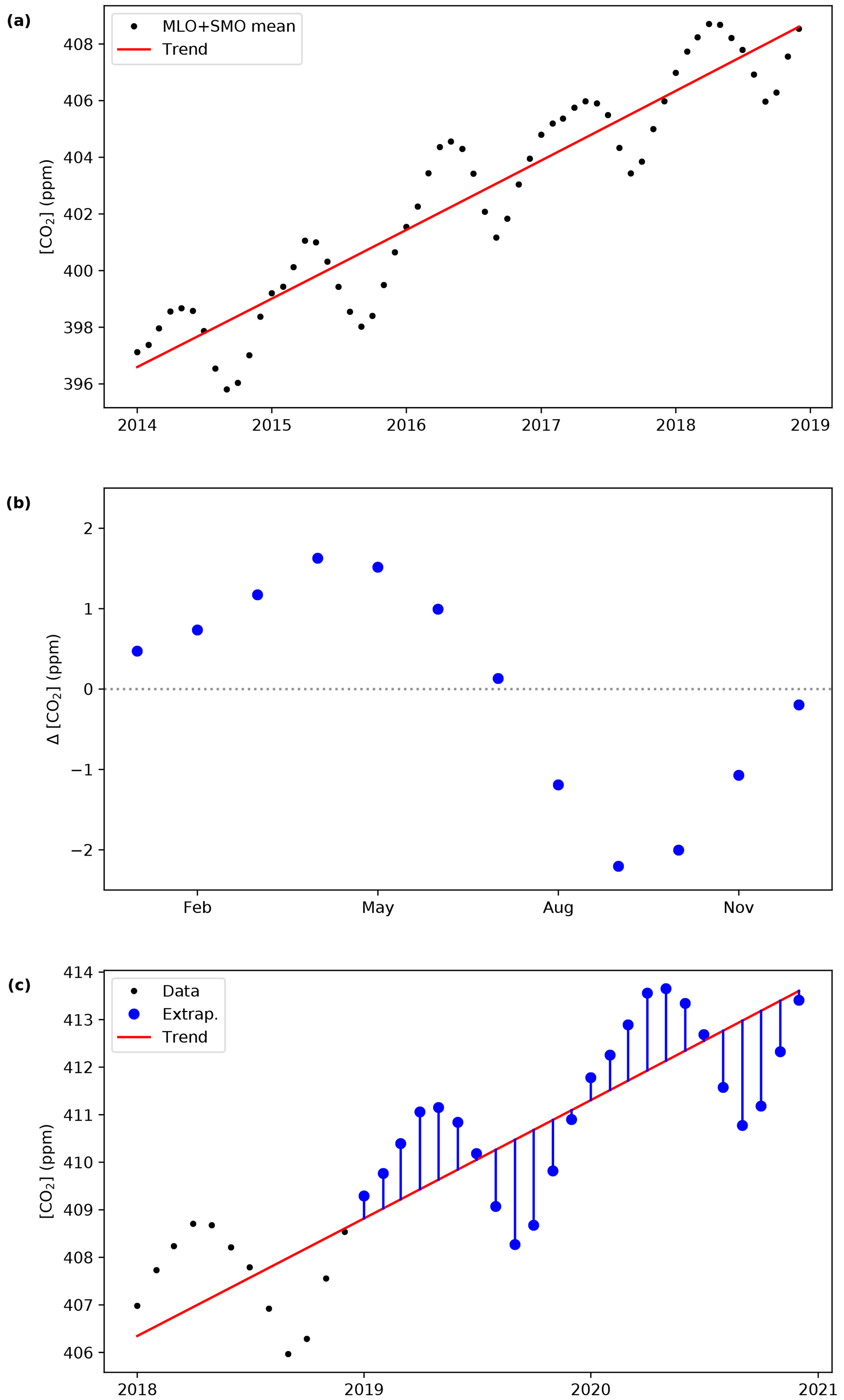
Figure 1 Process to extrapolate the combined MLO and SMO monthly average record. (a) First, we fit the last 5 or 10 years with the best function for a given gas. (b) Second, we calculate the mean monthly anomaly relative to the trend over the same time period. (c) Third, we extend the trend in time and apply the mean monthly anomalies on top of it.

Details of f(t) and n are provided in Table 1. Note that this method is also used to extrapolate back in time if data prior to the start of the combined MLO and SMO record are needed to represent the distribution of ages of air in the stratosphere (see Sect. 2.3).

Table 1 Function forms (f(t)) and number of years used to fit the combined MLO and SMO DMF record to extrapolate beyond 2018. In f(t), the c values are the fit parameters.

Errors in extrapolating the MLO and SMO DMFs will negatively impact the TCCON retrievals if the error in extrapolation introduces an error in the profile shape, for example, due to an El Niño year. In a scaling retrieval, such as the GGG algorithm used by TCCON, the posterior optimal profile is the prior profile multiplied by a scale factor, with the same scale factor applied to all levels. At its core, the algorithm we are describing here builds the priors by calculating what date to pull the MLO and SMO DMFs from for each level in the prior. If the extrapolation error caused all the MLO and SMO DMFs to be incorrect by the same percentage, this would manifest as the prior profile being incorrect by that percentage, for which a scaling retrieval can theoretically perfectly account. However, if the error in MLO and SMO DMFs is not the same for each level in the prior, the error in the prior cannot be represented by the same scalar multiplier for every level, and thus a scaling retrieval could never completely eliminate the error in the posterior profile.

Currently, we estimate the error in the MLO and SMO DMFs due to extrapolation to be about 0.25 % for CO₂, 0.15 % for N₂O, and 0.6 % for CH₄ over a 5-year extrapolation (see Sect. S2 in the Supplement for details). We deem this level of uncertainty acceptable for TCCON priors. How errors in the priors alias into the posterior state in a profile retrieval, such as that used by OCO-2 and -3, is more complex. However, the OCO-2/3 retrieval uses a relatively tight covariance matrix for levels in the stratosphere (see Fig. 3-15 of Crisp et al., 2021), making it important that the priors not exhibit any long-term drift in these levels. Therefore, when these priors are used for the version 11 OCO-2/3 retrievals, more recent NOAA data are ingested (see Sect. 4).

Ingesting the MLO and SMO data as the basis for the priors effectively ties those priors to the World Meteorological Organization (WMO) scale to which the MLO and SMO data are calibrated. Table 2 describes which scale each gas is tied to for each algorithm in which these priors are used. As these priors were developed at the same time as the X2019 CO₂ scale (Hall et al., 2021), whether the CO₂ priors are tied to the X2007 or X2019 CO₂ scale depends on which scale the MLO and SMO data are calibrated to.

Table 2 The WMO calibration scales to which the in situ data used in the GGG2020 and OCO-2/3 priors are tied.

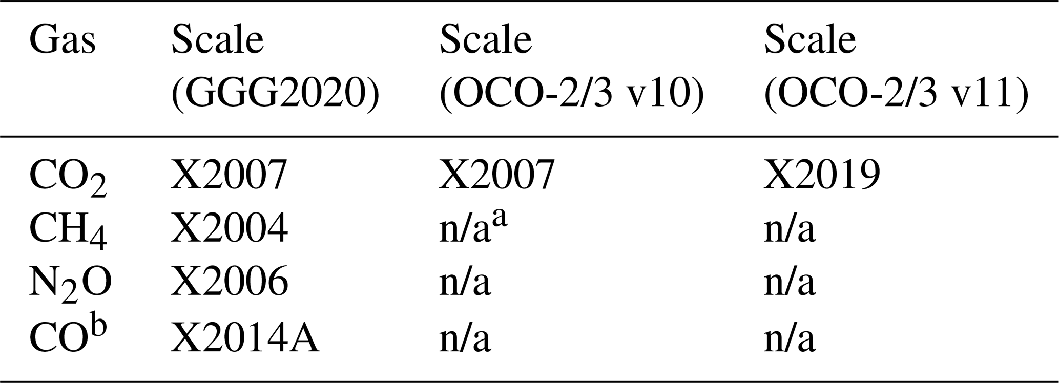
^a n/a​​​​​​​ stands for not applicable, as OCO-2 and OCO-3 only use CO₂ priors.​​​​​​​ ^b Note that, unlike for CO₂, N₂O, and CH₄ (for which this tie comes from the MLO and SMO data), for CO this is from scaling to ATom data in the troposphere.

Unlike the other gases in Table 2, CO is not tied to its scale through the MLO and SMO data. CO priors are created using a different approach to the other primary gases; this approach will be described in Sect. 3.6. The relevant point here is that CO is taken from the GEOS FP-IT product (Lucchesi, 2015), and in the troposphere it is scaled to match observations from the first three Atmospheric Tomography Mission (ATom) aircraft campaigns (Thompson et al., 2022). As the ATom quantum cascade laser spectrometer (QCLS) CO observations used were calibrated to the X2014A scale, the CO priors are considered tied to that scale.

Several gases (CO, H₂O, HDO, O₃) are contained in the GEOS FP-IT meteorology product ingested by GGG2020. H₂O and O₃ are taken directly from GEOS FP-IT, while CO and HDO are derived from GEOS FP-IT. Details are given in Sect. 3.

Finally there are a large number of gases that must be accounted for as interfering absorbers during retrievals of primary TCCON target gases. These gases use priors derived from climatological profiles from the summer at 35^∘ N. Details are given in Sect. 2.4.

2.1 Design rationale

In developing the GGG2020 priors, we had the following two guiding principles in mind.

1. First, we wanted to minimize direct dependence on other measurements or models as much as possible, such that retrievals using these priors are independent measurements (in the statistical sense) that other observations or models can be compared to.

2. Second, we wanted to produce an algorithm that generates reproducible prior profiles if run at different times.

The first principle is why the GGG2020 priors only ingest MLO and SMO data, rather than more surface data, and why we do not use modeled gas profiles (other than for CO). For the much shorter-lived CO, we decided that capturing the spatial variability was worth the trade-off of relying on GEOS FP-IT modeled CO (especially as GGG2020 already uses GEOS FP-IT meteorology). Other data used in generating the priors (e.g., latitudinal gradients of CO₂ and CH₄ from HIPPO and ATom, as well as Atmospheric Chemistry Experiment Fourier Transform Spectrometer, ACE-FTS, profiles) were likewise adopted because the improvement in the priors was deemed worth the loss of statistical independence. Since these data are used to generate static values (such as lookup tables or coefficients in functions), rather than for direct ingestion, we retain some independence from these sources.

The second principle is why the GGG2020 priors and OCO-2/3 v10 priors only use MLO and SMO flask data through the end of 2018 (rather than updating regularly). One concern raised during development was whether such regular data updates would alter previously obtained data, such as from retrospective quality control. This would introduce a situation where we could not exactly reproduce priors generated using an old version of the input data. Given time constraints, it was not possible to engineer a solution to detect or avoid this issue for GGG2020 and OCO-2/3 v10 priors. With the additional development time for OCO-2/3 v11, we were able to update the priors algorithm to safely ingest more rapidly updated MLO and SMO data.

2.2 Tropospheric prior

The GGG2020 tropospheric priors assume that the trend observed by MLO and SMO is driven by emissions in the northern midlatitudes; thus, the measured DMF at MLO and SMO will lag behind the DMFs in the Northern Hemisphere and precede the DMFs in the Southern Hemisphere. To compute the tropospheric DMFs, we average MLO and SMO data together with equal weight, deseasonalize the MLO and SMO average to get the underlying trend, approximate the offset forward or backward in time relative to MLO and SMO with an idealized distance function, apply a multiplicative and additive correction to match observed latitudinal gradients, and impose a latitudinally dependent seasonal cycle. Mathematically, this follows Eq. (1):

$$\begin{array}{}\text{(1)}& \begin{array}{rl}\mathrm{DMF}(l,z,z_{\mathrm{trop}},f_y)=& s(l,z,f_y,d)\\ & \cdot \left[\mathit{\alpha }\left(d\right)\cdot {\mathrm{DMF}}_{\mathrm{ref}}\left(d\right)+\mathit{\beta }\cdot l\right]\end{array}.\end{array}$$

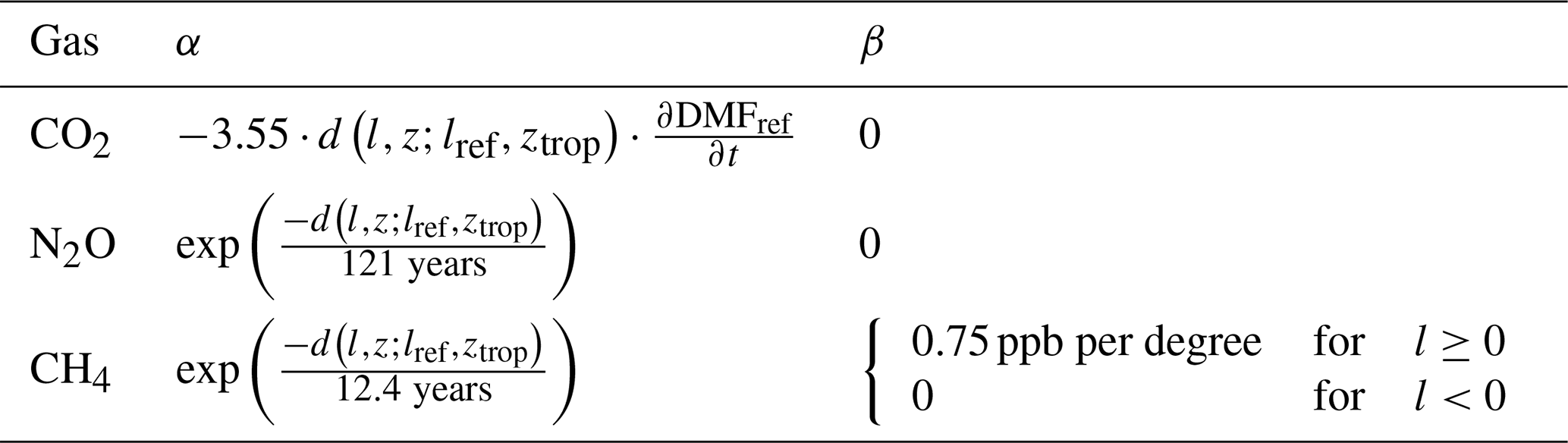
Table 3 Values of α and β coefficients in Eq. (1) for the three primary well-mixed gases. Rationales for these choices are given in the gas-specific sections (Sect. 3).

The variables in this function are as follows.

• l is latitude. In the GGG2020 TCCON priors, this is an “effective latitude” derived from mid-tropospheric potential temperature (see Sect. 2.2.1).

• z is altitude with the bottom half of the troposphere stretched downward slightly to treat the bottom layer as being at the surface for the purpose of this calculation (see Sect. 2.2.2).

• z_trop is the tropopause altitude.

• f_y is the fractional year (defined as 1-based day of year $/$ 365.25).

• DMF_ref is the reference DMF taken from a deseasonalized MLO and SMO trend.

• d is the distance offset function, defined by Eq. (2).

• s is the seasonal cycle factor, defined by Eq. (4d).

• α and β are coefficients that scale and adjust the ideal gradients assumed by d to account for differences between gases. Their values are given in Table 3 and are discussed in detail in Sect. 3.

The distance function d is shown in Fig. 2 (assuming a simple latitudinal dependence for the tropopause altitude). It has the following mathematical form:

$$\begin{array}{}\text{(2)}& d=d^{\prime }\left(l,z;l_{\mathrm{ref}},z_{\mathrm{trop}}\right)-d^{\prime }\left(\mathrm{0}{}^{\circ },\mathrm{0.01}\mathrm{km};l_{\mathrm{ref}},z_{\mathrm{trop}}\right),\end{array}$$

where

$$\begin{array}{}\text{(3)}& \begin{array}{rl}{d}^{\prime }(l,z;l_{\mathrm{ref}},z_{\mathrm{trop}})=& \mathrm{0.313}-\mathrm{0.085}\cdot \exp \left(-{\left[{\displaystyle \frac{l-l_{\mathrm{ref}}}{\mathrm{18}}}\right]}^{\mathrm{2}}\right)\\ & -\mathrm{0.268}\cdot \exp \left(-\mathrm{1.42}{\displaystyle \frac{z}{z+z_{\mathrm{trop}}}}\right)\\ & \cdot {\displaystyle \frac{l/\mathrm{22}}{\sqrt{\mathrm{1}+(l/\mathrm{22}{)}^{\mathrm{2}}}}}.\end{array}\end{array}$$

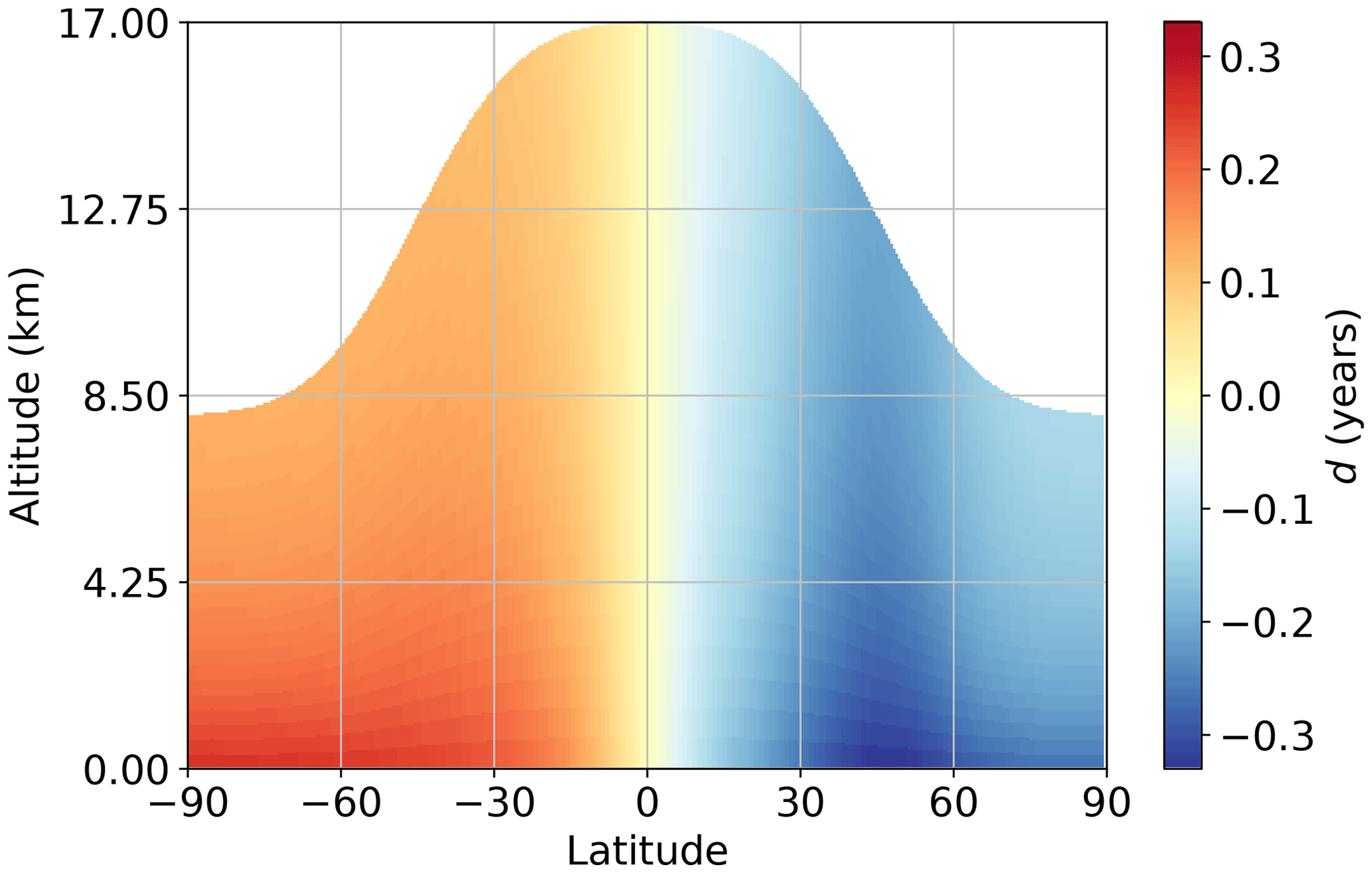
Figure 2 Form of the distance function d assuming that emissions occur at 45^∘ N and a latitudinally dependent tropopause height that varies smoothly from 17 km at the Equator to 8 km at the poles.

Although d has units of years, it does not represent a physical age or time. It is effectively a basis function to impose the ideal distribution of DMFs relative to MLO and SMO as shown in Fig. 2. Specifically, it assumes that surface DMFs precede MLO and SMO DMFs in the Northern Hemisphere, lag MLO and SMO DMFs in the Southern Hemisphere, and have a smaller latitudinal gradient in the upper troposphere due to faster winds. The basic shape is modified for each gas via α and β.

Figure 3 Parameterized seasonal cycle for (a) CO₂ and (b) CH₄. The left y axis is the factor s in Eqs. (4d) and (5d). The right y axis gives what the seasonal cycle amplitude would be for a CO₂ DMF of 400 ppm in (a) and CH₄ DMF of 1800 ppb in (b).

DMF_ref in Eq. (1) is the combined MLO and SMO record, deseasonalized by taking a 12-month rolling mean. This is done because the seasonal cycle at MLO and SMO is not representative of all latitudes. We impose a latitudinally dependent seasonal cycle by multiplying the DMFs by a scaling factor s:

$$\begin{array}{}\text{(4a)}& {\displaystyle }{s}_{\mathrm{v}}=\sin \left(\mathrm{2}\mathit{\pi }\cdot [f_y-\mathrm{0.78}]\right),\text{(4b)}& {\displaystyle }{s}_{\mathrm{l}}={\displaystyle \frac{s_{\mathrm{v}}\cdot l/\mathrm{15}}{\sqrt{\mathrm{1}+(l/\mathrm{15}{)}^{\mathrm{2}}}}},\text{(4c)}& {\displaystyle }{s}_{\mathrm{a}}=s_{\mathrm{l}}\cdot \exp \left(-d^{\prime }(l,z;l_{\mathrm{ref}},z_{\mathrm{trop}})/\mathrm{0.85}\right),\text{(4d)}& {\displaystyle }s=\mathrm{1}+s_{\mathrm{a}}\cdot c_{\mathrm{gas}},\end{array}$$

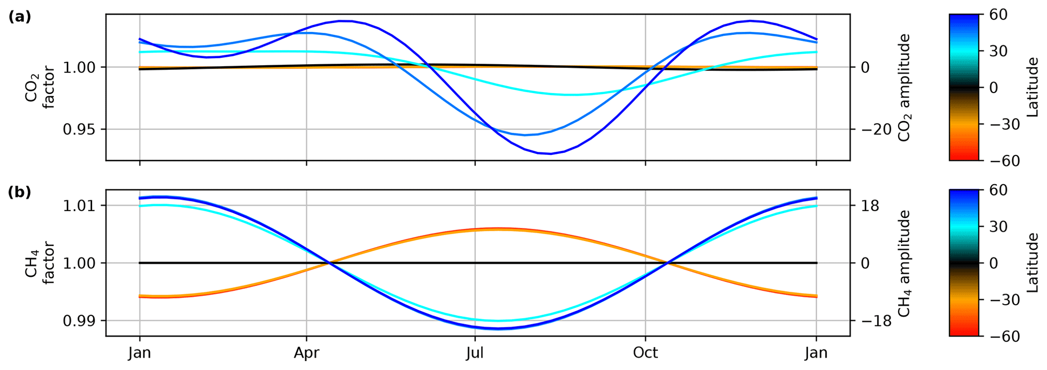
for all gases but CO₂. For CO₂ the parameterization is

$$\begin{array}{}\text{(5a)}& {\displaystyle }{s}_{\mathrm{v}}=\sin \left(\mathrm{2}\mathit{\pi }\cdot [f_y-\mathrm{0.834}-d]\right),\text{(5b)}& {\displaystyle }{s}_{\mathrm{l}}=s_{\mathrm{v}}+\mathrm{1.8}\cdot \exp \left(-{\left[{\displaystyle \frac{l-\mathrm{74}}{\mathrm{41}}}\right]}^{\mathrm{2}}\right)\cdot (\mathrm{0.5}-s_{\mathrm{v}}^{\mathrm{2}}),\text{(5c)}& {\displaystyle }\begin{array}{rl}{s}_{\mathrm{a}}=& s_{\mathrm{l}}\cdot \exp \left(-d/\mathrm{0.2}\right)\\ & \cdot \left\{\mathrm{1}+\mathrm{1.33}\cdot \exp \left(-{\left[{\displaystyle \frac{l-\mathrm{76}}{\mathrm{48}}}\right]}^{\mathrm{2}}\right)\cdot {\displaystyle \frac{z+\mathrm{6}}{z+\mathrm{1.4}}}\right\}\end{array},\text{(5d)}& {\displaystyle }s=\mathrm{1}+s_{\mathrm{a}}\cdot c_{\mathrm{gas}},\end{array}$$

where f_y is the fraction of year passed (defined as 1-based day of year $/$ 365.25), l is latitude, z is altitude (in kilometers), z_trop the tropopause altitude (in kilometers), l_ref is a reference latitude (45^∘ N), d^′ is the function from Eq. (3), and c_gas is a gas-specific constant defined in Table S5. s_v represents the basic seasonal variation, s_l the latitudinal variation, and s_a the altitude variation. The form of these equations for CO₂ and CH₄ are shown in Fig. 3.

These parameterized seasonal cycles are the same as those used in GGG2014 priors. The amplitude and phase were derived from surface in situ data, and the amplitude is assumed to decay with altitude due to mixing of air masses with different ages.

2.2.1 Potential temperature-based effective latitude

CO₂ profiles for locations on the edge of the tropics are sometimes more “tropical” in nature than their geographic latitudes suggest. In these cases, the observed profile would be more constant versus altitude than the prior profile, which would have some drawdown at the surface.

Keppel-Aleks et al. (2012) showed that, in the extratropics, there is a correlation between 700 hPa potential temperature and CO₂ DMFs in the free troposphere, as variations in this potential temperature serve as an indicator of synoptic-scale motion and therefore the true source latitude of the air. We use dry potential temperature, i.e., the temperature a parcel of dry air would have if brought to a pressure of 1000 hPa adiabatically. This allows us to use potential temperature to derive an “effective latitude” that better predicts the shape of the prior profile. Note that while this was originally developed to improve the CO₂ priors, it is used for all gases.

To calculate this effective latitude, we first build a climatology of mid-tropospheric potential temperature from the GEOS FP-IT product by averaging potential temperature between 500 and 700 hPa (henceforth termed θ_mid) versus latitude for 2-week periods in 2018 (Fig. 4a). A hypothetical example is shown in Fig. 4b. For a prior in the extratropics, we select the appropriate θ_mid versus latitude curve from the climatology (Fig. 4b, black line) and compare the θ_mid value for the prior against the tabulated mean. If the prior's θ_mid is greater than the mean θ_mid for that latitude, the effective latitude is moved equatorward until it matches (vice versa if the prior's θ_mid is less).

Figure 4 (a) The lookup table for θ_mid versus latitude and time of year. (b) A hypothetical example of how the effective latitude calculation works. The black line represents the climatological θ_mid, and the black points represent hypothetical θ_mid for individual profiles'. The arrows indicate how the effective latitude of each profile is adjusted such that the individual θ_mid matches the climatological θ_mid. The red shading indicates latitudes where this method is not applied; the blue shading indicates transitional areas between the geographic and effective latitude (see Sect. 2.2.1 for additional details).

More specifically, the implementation searches north and south of the prior's geographic latitude for the two latitudes (one north, one south) with the smallest difference between the prior's θ_mid and the mean θ_mid. If the difference between the mean θ_mid values at both latitudes is within 0.25 K, then the nearer latitude is used. Otherwise, the latitude with the smallest difference between its θ_mid and the prior's θ_mid is used.

There are two caveats to this approach. First, the effective and true (geographic) latitude must have the same sign – that is, both must be in the same hemisphere. Second, within the tropics (defined as within ±20^∘ of the Equator), the effective latitude calculation is disabled and the geographic latitude is used. This is done because mid-tropospheric temperature gradients are weak in the tropics and largely uncorrelated with zonal advection (Sobel et al., 2001). To smoothly blend between geographic and effective latitude, a linear interpolation between them occurs in the 20 to 25^∘ range. For example, a profile at 22^∘ N would have a latitude calculated as 0.6l_g+0.4l_e, where l_g is the geographic latitude and l_e is the effective latitude.

2.2.2 Altitude grid adjustment

The seasonal cycle and distance basis function assume that the surface is at 0 km altitude. To this end, we use an adjusted altitude as z in Eqs. (1) through (5d). To compute this adjusted z, we stretch or squeeze the bottom of the altitude grid so that the bottom layer is at the surface altitude from the GEOS FP-IT 2D files. The adjustment is performed as follows:

$$\begin{array}{}\text{(6)}& z_{\mathrm{adj}}=\left\{\begin{array}{lll}{z}_{\mathrm{orig}}& \text{if}& z_{\mathrm{orig}}\ge z_{\mathrm{blend}}\\ z_{\mathrm{orig}}+\mathrm{d}z\cdot f^{\mathrm{2}}& \text{if}& z_{\min }\le z_{\mathrm{orig}}\le z_{\mathrm{blend}}\\ \mathrm{0}& \text{if}& z_{\mathrm{orig}}<z_{\min }\end{array},\right.\end{array}$$

where z_orig is the original altitude, $\mathrm{d}z=z_{\mathrm{surf}}-z_{\min }$, z_min is the original grid altitude closest to z_surf, z_blend is the original grid altitude closest to $z_{\mathrm{surf}}+\frac{\mathrm{1}}{\mathrm{2}}\cdot (z_{\mathrm{trop}}-z_{\mathrm{surf}})$, z_surf is the GEOS FP-IT surface altitude, z_trop is the tropopause altitude, and f is

$$\begin{array}{}\text{(7)}& f={\displaystyle \frac{i_{\mathrm{blend}}-i}{i_{\mathrm{blend}}-i_{\min }}},\end{array}$$

where i_blend, i_min, and i are the indices for z_blend, z_min, and z, respectively. Figure S7 shows an example of the adjustment. This adjustment is minor (typically 50 to 100 m) since the priors are generated on the terrain following levels from the GEOS FP-IT model.

2.3 Stratospheric prior

The design of the stratospheric priors draws heavily from Andrews et al. (2001a). That work showed that the profiles of CO₂ and N₂O in the lower stratosphere can be captured well using surface in situ data from the MLO and SMO observatories to determine the trace gas mole fraction entering the stratosphere and then accounting for mixing of air during stratospheric circulation. We extend this method by using atmospheric profile measurements between February 2004 and March 2019 from the Atmospheric Chemistry Experiment Fourier Transform Spectrometer (ACE-FTS, Bernath et al., 2005), data version 3.6 (Boone et al., 2013), to capture chemical production and/or loss of N₂O and CH₄ and production of HF.

2.3.1 Stratospheric age of air

The age of stratospheric air parcels is calculated from a climatology simulated by the Chemical Lagrangian Model of the Stratosphere (CLaMS) and scaled to match the mean midlatitude age in the Goddard Space Flight Center 2D (GSFC2D) model (Fleming et al., 2011), which provides age of air as a function of latitude, potential temperature, and day of year. Age of air in this context refers to the time since the air entered the stratosphere. Figure 5 shows both latitudinal and temporal slices of the CLaMS age of air. The CLaMS model is a 2D representation of the mean dynamics of the stratosphere. To account for the zonal displacements driven by large-scale Rossby waves, we compute an equivalent latitude profile. Equivalent latitude is derived from PV following Eq. (1) in Allen and Nakamura (2003).

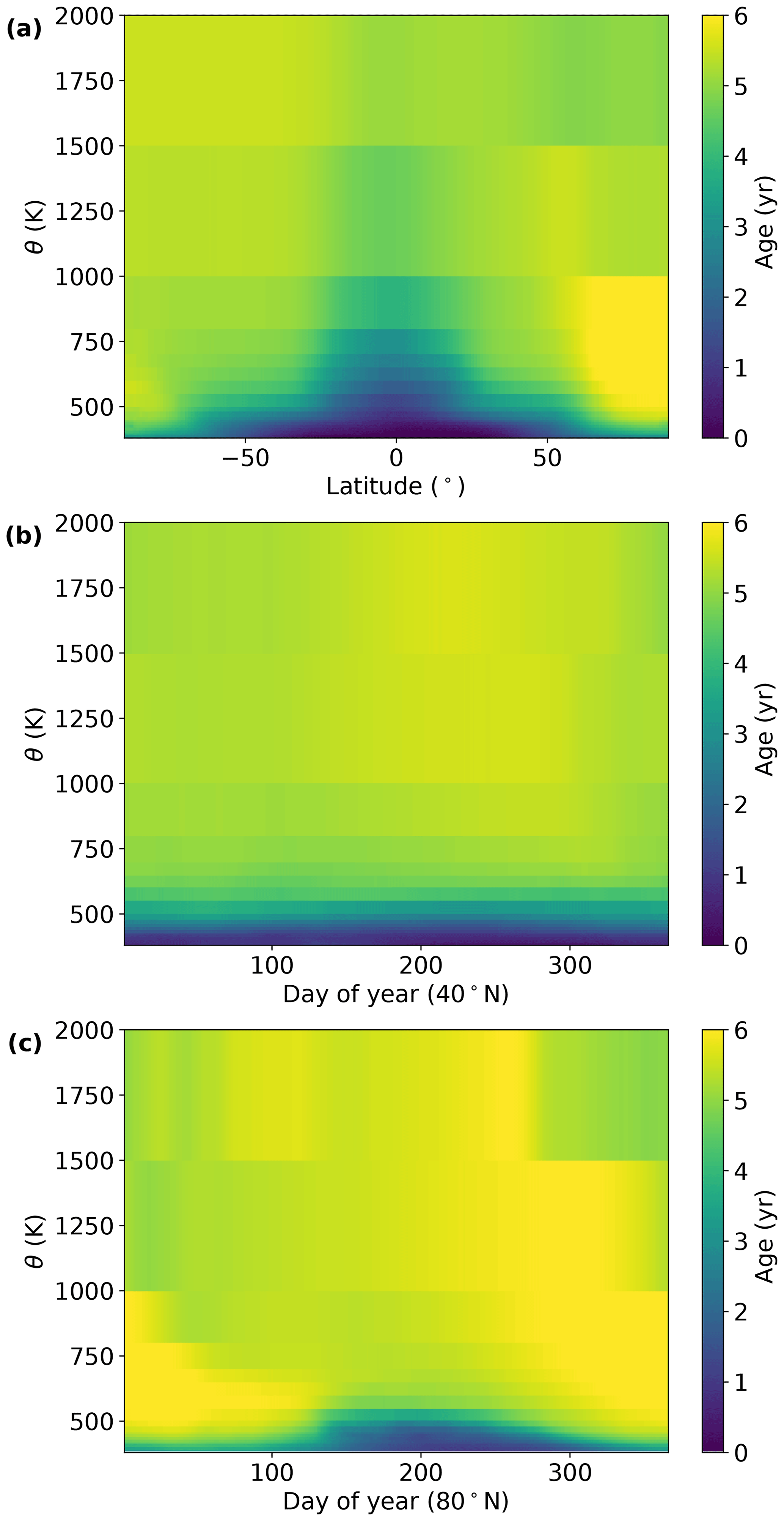
Figure 5 Mean age of air from the CLaMS climatology. (a) Age versus latitude and potential temperature for 1 January, (b) age versus day of year and potential temperature at 40^∘ N. Panel (c) is the same as panel (b) but for 80^∘ N.

Note that this equivalent latitude is not the same as the effective latitude used in the tropospheric part of the prior calculation. PV-derived equivalent latitude has been previously shown to predict stratospheric chemical fields well (e.g., Allen and Nakamura, 2003), while a coordinate derived from mid-tropospheric potential temperature predicts synoptic variation in tropospheric trace gas mixing ratios (e.g., Keppel-Aleks et al., 2012). Therefore, we use the PV-derived equivalent latitude here for the stratospheric part of the priors and potential temperature-derived effective latitude in Sect. 2.2.1 for the tropospheric part of the priors.

2.3.2 Age spectra and chemistry

Once the age of air is known, we can look backwards in the combined MLO and SMO record to determine the stratosphere boundary condition (SBC), i.e., the mole fraction of each gas when a parcel of air entered the stratosphere. The SBC time series is defined as the MLO and SMO average lagged by 2 months; Andrews et al. (2001a) and references therein show that this is a good proxy for the SBC. However, the mole fraction for a given level in the prior is not simply the mole fraction of, e.g., CO₂, when that air entered the stratosphere but is the result of mixing of air with different ages during convective transport. This mixing can be represented by solutions to Green's function derived from CO₂ measurements (Andrews et al., 2001a), which we represent as age spectra.

Age spectra were precomputed for three regions (tropics, midlatitudes, and polar vortex) and ∼ 45 different mean ages. Andrews et al. (1999, 2001b) showed that different age spectra were necessary to capture tropical and midlatitudinal behavior; likewise, the polar vortex requires its own age spectra form due to strong wintertime descent of air. Example age spectra are shown in Fig. 6. Note that spectra for the youngest mean ages are not shown.

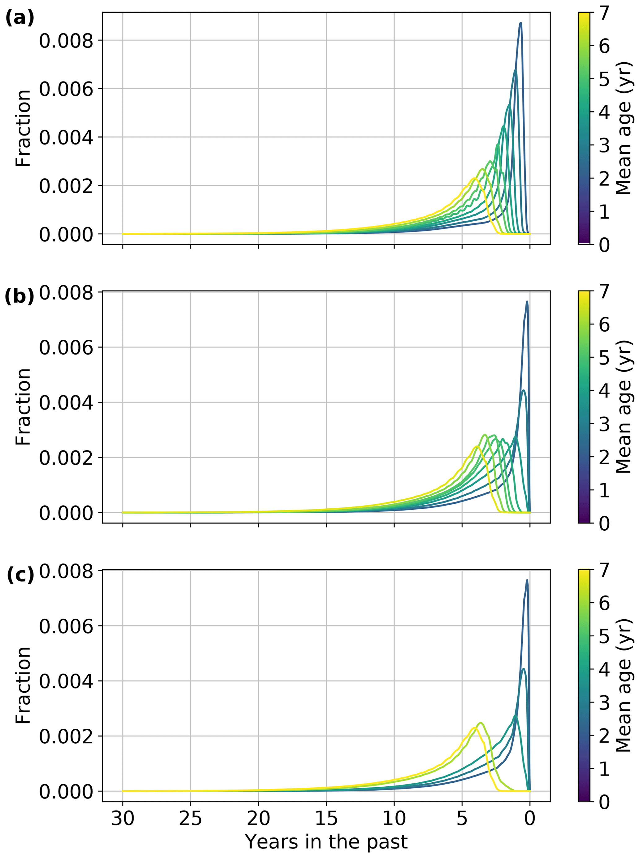
Figure 6 Example age spectra for the (a) tropics, (b) midlatitudes, and (c) polar vortex. The y values represent the contribution of air from that time to the average mole fraction of the parcel as a whole. Note that age spectra for the youngest air are not shown because they are nearly delta functions.

For each stratospheric level in the priors, the mole fraction of a gas is computed as

$$\begin{array}{}\text{(8)}& \stackrel{\mathrm{‾}}{c}=\stackrel{\mathrm{‾}}{F}(a,\mathit{\theta })\int S_{a,r}\left(t\right)c\left(t\right)\mathrm{d}t,\end{array}$$

where S_a,r(t) is the value of the age spectrum for the given mean age (a) and region (r) and c(t) is the SBC, both at time t. That is, the mole fraction is a weighted average of the SBC over time with the weights set by the age spectrum. $\stackrel{\mathrm{‾}}{F}(a,\mathit{\theta })$ is the fraction of gas remaining after chemical loss, and θ is potential temperature, which we use as a vertical coordinate. For CO₂ this fraction is always 1, but it varies with mean age and potential temperature for other gases, as discussed in more detail in Sect. 3.

2.3.3 Middleworld treatment

The middleworld is defined as the part of the atmosphere between the tropopause pressure from GEOS FP-IT and the 380 K isentrope. Of the three tropopause pressure estimates in GEOS FP-IT, we use the blended (thermal and potential vorticity) estimate. The 380 K isentrope is the lowest potential temperature surface entirely contained within the stratosphere; therefore, the stratospheric approach described in Sect. 2.3 is only applicable to levels above 380 K (the stratospheric overworld). To fill in the prior in the middleworld, we linearly interpolate mole fraction as a function of potential temperature between the tropopause and 380 K.

2.4 Secondary gases

For the purpose of this paper, “secondary gases” are defined as those which are tied directly to neither the MLO and SMO records nor the GEOS FP-IT product. This is all gases other than CO₂, N₂O, CH₄, HF, CO, H₂O, HDO, and O₃. O₂ and HCl are the two most relevant to standard TCCON retrievals. Priors for these gases are based on climatological profiles for summer at 35^∘ N derived from profiles measured by MkIV spectrometer balloon flights (Toon, 1991) and the ACE-FTS instrument. These climatological profiles are modified for a given location and time in four steps:

1. stretch or compress the profile vertically so that the tropopause is at the correct altitude,

2. apply a latitudinal gradient,

3. apply a secular trend,

4. apply a seasonal cycle.

These steps require the latitude and age of air of the profiles. This approach is nearly identical to that used for all gases in the GGG2014 priors, except that for steps 2–4 the age of air and effective latitude described in Sect. 2.2 are used in the troposphere and the CLaMS age and PV-derived equivalent latitude from Sect. 2.3 are used in the stratosphere. The middleworld is filled in by linear interpolation in θ between the tropopause and 380 K, as is done for the primary gases. Details of the calculation are given in the Supplement.

2.5 Conversion to number density

All trace gas quantities shown and discussed in this paper are in dry mole fractions (DMFs, i.e., moles of trace gas per moles of dry air). However, in its forward model, GGG uses gas profiles in number density (molec. cm⁻³) for spectroscopic calculations. To convert DMF to number density, we use

$$\begin{array}{}\text{(9)}& n_{\mathrm{gas}}={\displaystyle \frac{c_{\mathrm{gas}}}{\mathrm{1}+c_{{\mathrm{H}}_{\mathrm{2}}\mathrm{O}}}}{n}_{\mathrm{ideal}},\end{array}$$

where n_gas is the number density of the gas of interest, c_gas is the DMF of that gas, $c_{{\mathrm{H}}_{\mathrm{2}}\mathrm{O}}$ is the DMF of water (from the H₂O prior profile), and n_ideal the ideal gas number density. The factor $\mathrm{1}+c_{{\mathrm{H}}_{\mathrm{2}}\mathrm{O}}$ converts n_ideal into number density of dry air.

3 Gas-specific design

In this section, we will discuss elements of the algorithm unique to each gas. With the exception of O₂, each section will be divided into subsections for the tropospheric and stratospheric priors.

3.1  O₂

We assume a uniform DMF of 0.2095 for O₂ at all altitudes. During the retrieval, this is converted to number density following Sect. 2.5. In the GGG2014 priors, the conversion to number density did not include a correction for water. This led to a profile shape error: as water DMFs are highest near the surface, failing to include the water correction led to an overestimate of the near-surface number density for every absorbing gas.

The impact of this error in the previous priors on the final column amounts was small because in public TCCON data all gas column amounts are reported as column average mole fractions (termed Xgas, e.g., XCO₂). These are calculated as follows:

$$\begin{array}{}\text{(10)}& \mathrm{Xgas}={\displaystyle \frac{V_{\mathrm{gas}}}{V_{{\mathrm{O}}_{\mathrm{2}}}/\mathrm{0.2095}}},\end{array}$$

where V_gas and $V_{{\mathrm{O}}_{\mathrm{2}}}$ are the total column amounts (in molec. cm⁻²) of the target gas and O₂, respectively. The denominator represents a column of dry air inferred from the retrieved O₂ column. The advantage of this method over using a column of air derived from surface pressure is that, because primary TCCON target gases are measured on the same detector as O₂, certain types of instrumental error cancel out in this ratio, reducing their impact on the final data product (Washenfelder et al., 2003; Wunch et al., 2011). Likewise, the shape error due to the missing water correction in GGG2014 priors largely canceled out in the column-averaged Xgas DMFs. However, the GGG2020 treatment, following Eq. (9), is more physically consistent, leads to more consistent O₂ scaling factors retrieved among TCCON stations, and yields a better shape – especially under warm, humid conditions.

3.2  CO₂

3.2.1 Troposphere

The value of α in Eq. (1) for CO₂ was derived by comparing the priors generated with α=1 and β=0 against profiles from the HIPPO (Wofsy, 2011) and ATom (Wofsy et al., 2021; Thompson et al., 2022) campaigns. We used CO₂ measurements from the Harvard quantum cascade laser spectrometer (QCLS) for HIPPO and CO₂ measurements from the NOAA Picarro for ATom. Only data from individual vertical profiles (identified as data points where the PFP/prof.no variable is >0 in the merge files from https://doi.org/10.3334/ORNLDAAC/1925, Wofsy et al., 2021) with ≥ 10 valid data points were used. The differences between the priors and observations below 800 hPa were averaged over 20^∘ latitude bins and converted from units of parts per million to multiples of the interannual CO₂ growth rate, derived from the MLO and SMO average deseasonalized trend. The output of the distance function d (Eq. 2) was also averaged for all prior levels below 800 hPa and binned to 20^∘ latitude bins.

The result is shown in Fig. 7a. The red line is a York fit (York et al., 2004) to the data using the inverse square of the standard deviations of the prior–observation differences and distance function values in the latitude bins as the weights. This fit indicates setting α equal to −3.55 times the CO₂ interannual growth rate will give a latitudinal gradient that matches observations. Figure 7b shows the mean differences versus latitude with α set to 1 (i.e., no adjustment) and with the best fit to the data. Using the α derived from Fig. 7a and β=0, the priors show no latitudinal bias versus observations.

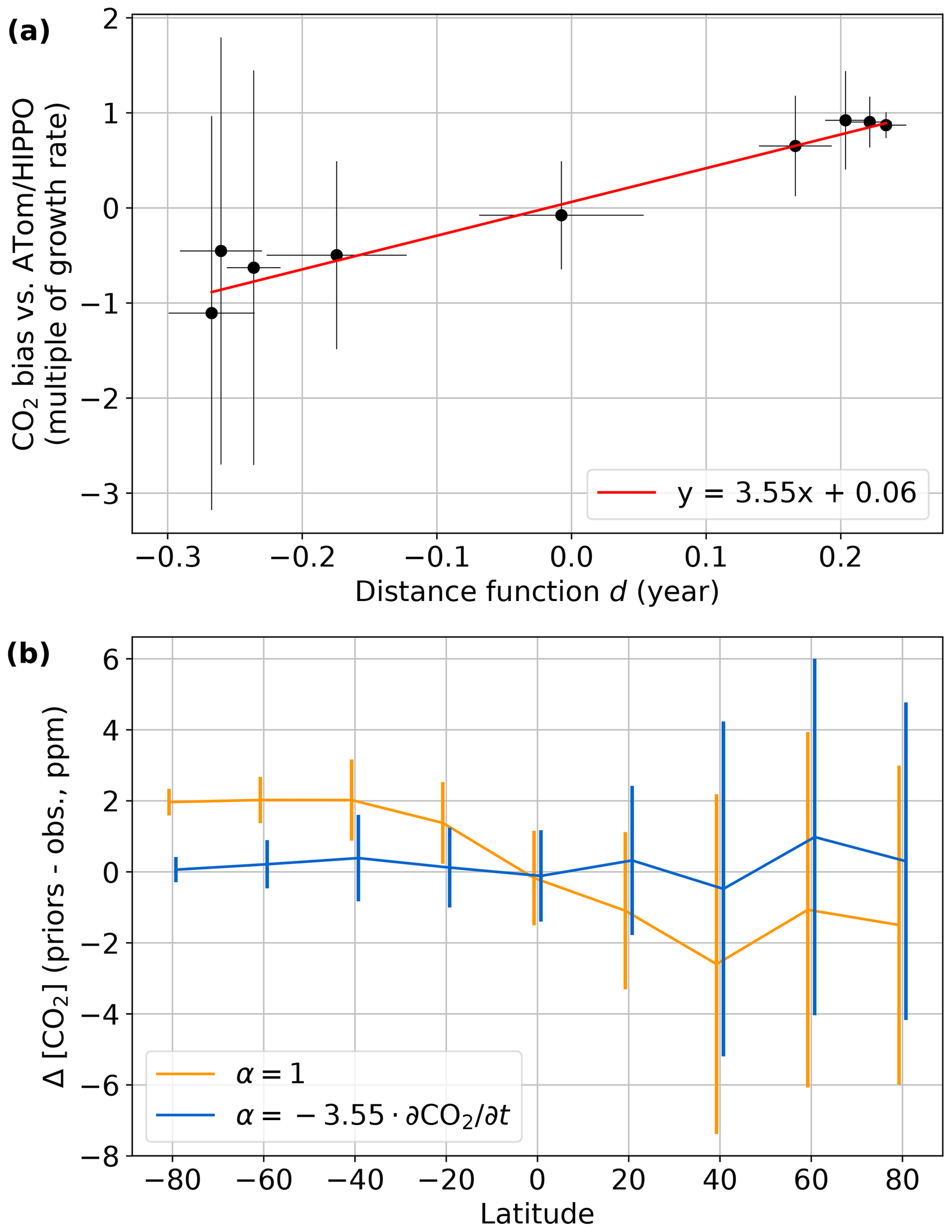
Figure 7 (a) Bias between the initial CO₂ DMFs and ATom/HIPPO profile versus the distance function (Eq. 2) for profile levels below 800 hPa. Note that the y axis is not in parts per million but in multiples of the interannual CO₂ growth rate. See Sect. 3.2.1 for details. (b) The mean difference between priors and observations in 20^∘ latitude bins below 800 hPa versus latitude bin center. In both panels, error bars are 1σ standard deviations of the respective variable within the 20^∘ latitude bins.

3.2.2 Stratosphere

CO₂ follows the algorithm laid out in Sect. 2.3. No additional modifications were required. For our purposes, we assume that CO₂ DMFs are unaffected by stratospheric chemistry (e.g., CH₄ oxidation) and do not include a correction for chemistry in stratospheric CO₂.

3.3  N₂O

3.3.1 Troposphere

We set α in Eq. (1) to

$$\begin{array}{}\text{(11)}& \exp \left({\displaystyle \frac{-d}{\mathit{\tau }}}\right),\end{array}$$

where d is the output of the distance function from Eq. (2) and τ=121 years (the mean atmospheric lifetime of N₂O, following Myhre et al., 2013, Table 8.A.1). This imposes a slight additional north–south gradient to N₂O in the troposphere.

3.3.2 Stratosphere

In the stratosphere, N₂O is more complicated than CO₂ because it is removed, principally through photolysis forming nitrogen N₂ and an oxygen atom O but also via a reaction with excited oxygen (O(¹D)) (Jacob, 1999). Andrews et al. (2001a) fit this loss of N₂O in the lower stratosphere versus age of air with a third-order polynomial. We examined how this polynomial compares to N₂O data from the ACE-FTS instrument (Bernath et al., 2005) and found that the polynomial's skill in predicting the fraction of N₂O remaining relative to the SBC (F(N₂O)) decreased above approximately 25 km altitude, with the polynomial overestimating the N₂O mixing ratio by up to 150 ppb. We hypothesize this is due to different chemistry in the upper stratosphere compared to the lower stratosphere. As the original polynomial was based on lower stratospheric data, it did not capture this behavior. While the fraction of the N₂O column in the upper stratosphere is small (a few percent above 20 km), our goal was to develop priors with reasonably accurate DMFs at all altitudes, not just where the bulk of the column mass is. Additionally, developing our own method to estimate F(N₂O) allows us to be consistent when calculating the same quantity for CH₄ and HF.

We use N₂O data from the ACE-FTS instrument to build a lookup table of the fraction of N₂O remaining as a function of age of air and potential temperature. Strong et al. (2008) validated a previous version of the ACE-FTS N₂O data and found that mean differences between ACE-FTS and other stratospheric N₂O measurements were ±10 ppbv between 18 and 30 km, and mostly within −2 to +1 ppbv between 30 and 60 km. They note that these are large relative to the magnitude of N₂O mole fractions at these altitudes; however, for our purposes, these are acceptable, given that we are averaging a large number of ACE-FTS profiles and need only a climatological relationship between fraction of N₂O remaining, age of air, and potential temperature. Waymark et al. (2014) compared the version 3 ACE-FTS data (used in this work) to the version 2 evaluated by Strong et al. (2008) and note that the main difference is a 10 % reduction in N₂O above 30 km. Thus the general results in Strong et al. (2008) should still hold. For ACE-FTS v3.5 data (one minor version earlier than that used in this work), Sheese et al. (2017) found biases between ACE-FTS and MIPAS (Michelson Interferometer for Passive Atmospheric Sounding) of between −9 % and 5 % and between ACE-FTS and MLS (Microwave Limb Sounder) of between −18 % and 4 % in the altitude range of 19 to 34 km.

To build the lookup table, age of air is computed as in Sect. 2.3; for each ACE profile, the stratospheric equivalent latitude is computed for the GEOS FP-IT files that bound it in time, and then it is interpolated to the latitude, longitude, and time of the profile. This equivalent latitude and the potential temperature calculated from ACE-FTS temperature and pressure is used as input to the CLaMS model from Sect. 2.3 to look up the age of air.

F(N₂O) is defined relative to the stratospheric boundary condition in the ACE-FTS data, not the MLO and SMO record, to ensure self-consistency and avoid introducing error from the bias between the ACE-FTS and MLO and SMO data (Fig. S9). The stratospheric boundary condition is computed from a quadratic fit in time of ACE-FTS N₂O data in the tropics (latitude within ±20^∘) and with 360 K < θ < 390 K, excluding outliers (defined as values more than 5 times the median deviation from the median). This definition of the stratospheric boundary condition assumes that most of the air entering the stratosphere does so in the tropics and that the tropical tropopause is in that range of potential temperature values.

Finally, to compute the F(N₂O) lookup table, the ACE-FTS data are binned by age of air (0.25 year increments) and potential temperature (variable increments; 50 K in the lower stratosphere to 200 K in the upper stratosphere). ACE-FTS data are excluded if

• F(N₂O)<0,

• altitude ≥ 70.0 km (this is the top altitude in the TCCON priors),

• the profile is in the polar vortex,

• potential temperature is <380 K (as we are only concerned with levels in the stratospheric overworld).

Additionally, F(N₂O) values > 1 are limited to 1. The resulting lookup table is shown in Fig. 8. As there are large gaps in age–θ space with no ACE-FTS data, we extrapolate to fill in these gaps. We use essentially a constant value extrapolation along age; that is, if there is no value for a given age–θ bin, the nearest point at the same θ is used. Linear extrapolation along age is done second, using the nearest two points to determine the slope. In general, points in these extrapolated regions are expected to be very infrequent, as the absence of ACE data suggests that those combinations of age and θ are rare in the atmosphere.

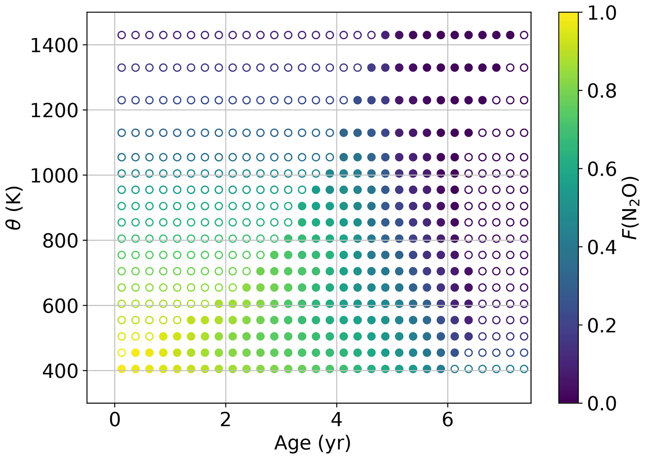
Figure 8 F(N₂O) lookup table derived from ACE-FTS v3.6 data as a function of potential temperature and age of air. Unfilled circles are extrapolated points.

The need to capture how F(N₂O) depends on both age and θ is apparent in Fig. 8. Consider the points in Fig. 8 at ages of 5 years. Over the range of 1000 K, the F(N₂O) decreases from ∼ 0.5 to almost 0. This is likely because at greater θ (i.e., higher altitude) the N₂O photolysis (${\mathrm{N}}_{\mathrm{2}}\mathrm{O}+h\mathit{\nu }\to {\mathrm{N}}_{\mathrm{2}}+\mathrm{O}$) pathway proceeds more rapidly than at lower altitudes. Age of air alone cannot capture this difference.

3.4  CH₄

3.4.1 Troposphere

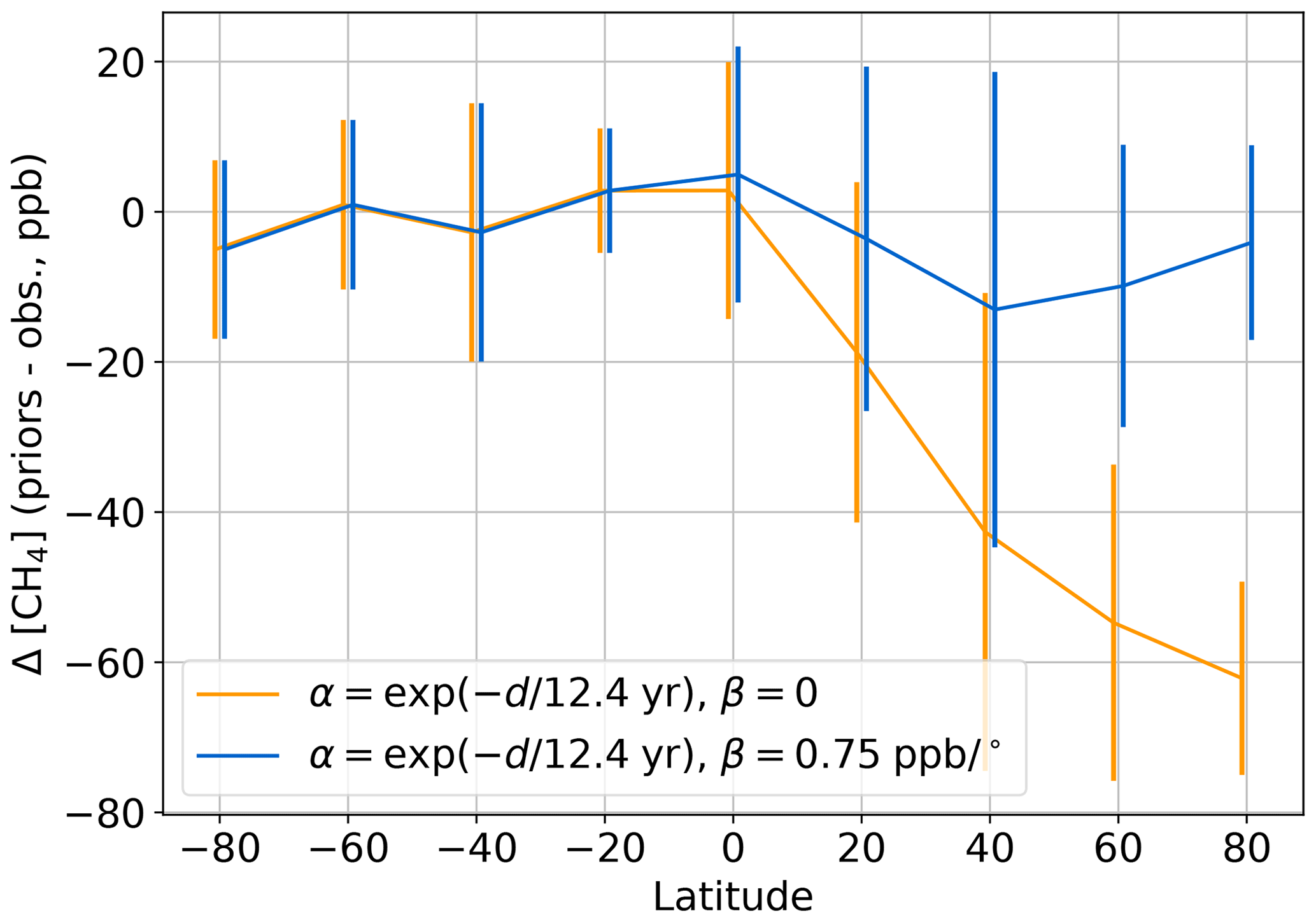
Similar to N₂O, the CH₄ priors use Eq. (11) as α, with a lifetime of 12.4 years (Myhre et al., 2013, Table 8.A.1). The orange line in Fig. 9 shows the mean prior versus observation differences below 800 hPa in 20^∘ latitude bins, as in Fig. 7b. A latitudinal bias in tropospheric methane mole fractions in the Northern Hemisphere remains. Therefore, we set β to 0.75 ppb per degree in the Northern Hemisphere, which removes this bias (blue line, Fig. 9).

Figure 9 Differences in CH₄ between ATom and HIPPO observations and priors, binned as in Fig. 7b, with and without β=0.75 ppb per degree correction in the Northern Hemisphere. Error bars are 1σ standard deviations in the 20^∘ latitude bins.

3.4.2 Stratosphere

CH₄ must also include a fraction remaining term, F(CH₄), to account for stratospheric chemistry, similarly to N₂O. Figure 10a shows a tight correlation between ACE-FTS N₂O and CH₄ in the stratosphere; therefore, we can use the relationship between F(N₂O) and age derived in Sect. 3.3 as a basis for the F(CH₄) lookup table.

Figure 10 (a) 2D histogram of F(N₂O) and F(CH₄) from ACE-FTS. (b) The F(CH₄) lookup table that is used in the GGG2020 algorithm. The same as in Fig. 8, filled circles are derived directly from data, while the unfilled circles are extrapolated. F values are computed as described in Sect. 3.3.

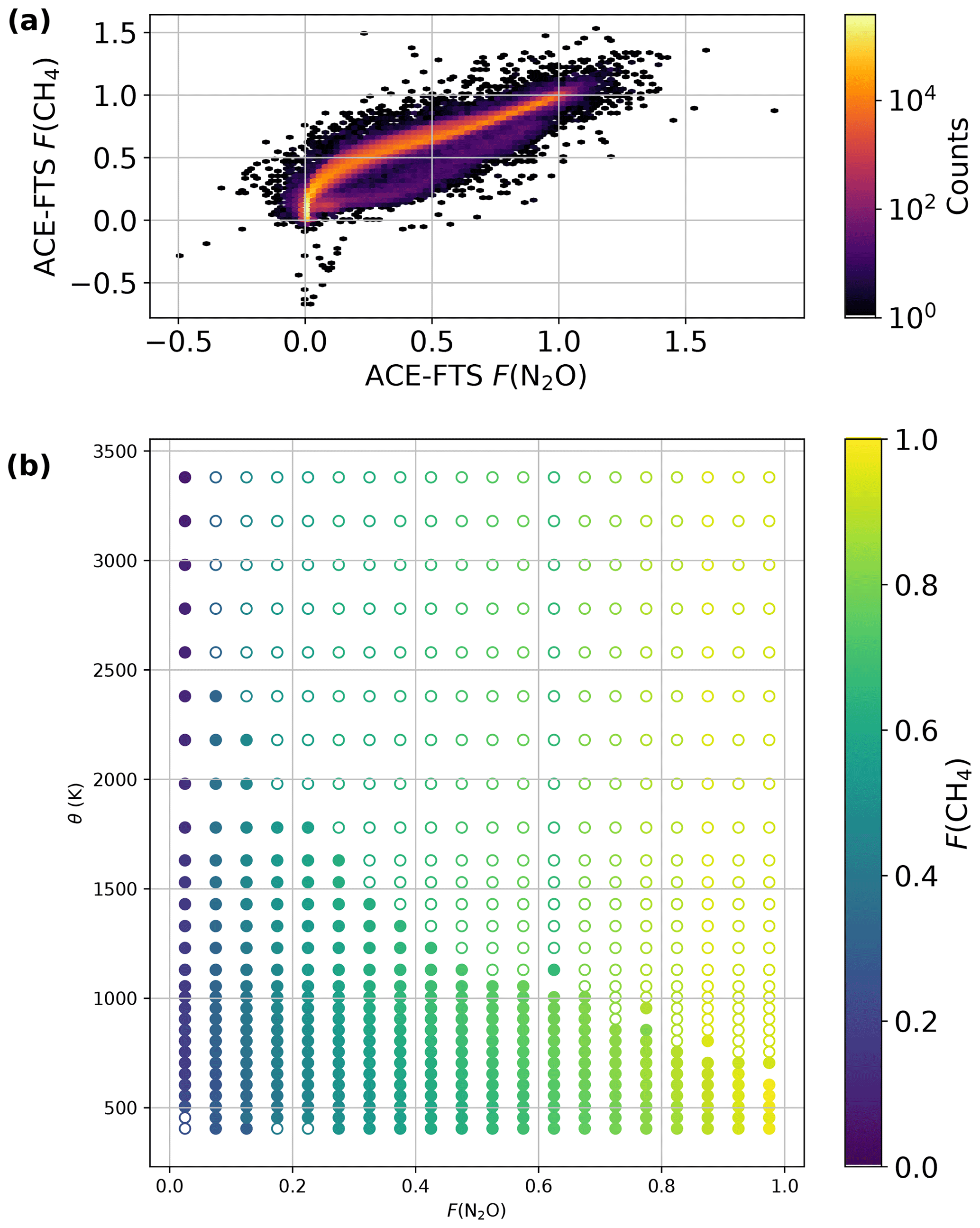
To compute the lookup table, we first limit the ACE-FTS data to points where F(N₂O) and F(CH₄) are positive, the CH₄ mole fraction is < 2000 ppb (points ≥ 2000 ppb are almost certainly tropospheric), the profile is outside the polar vortex, and the altitude is below 70 km. We bin the data by F(N₂O) and θ. Within each F(N₂O) bin, outliers are rejected (distance $\ge \mathrm{5}\times$ median absolute deviation) and the mean F(CH₄) value in each F(N₂O) and θ bin pair is computed. As with N₂O, we use extrapolation to fill in parts of the lookup table not covered by ACE-FTS data. We use constant value extrapolation along the θ dimension first, then also along the F(N₂O) dimension if necessary.

To compute the stratospheric prior profiles, Eq. (8) is used with the F(CH₄) value described above. To compute the F(CH₄) value, the age and θ values are first used to compute the F(N₂O) value as described in Sect. 3.3, and then the F(CH₄) value is determined by linearly interpolating the lookup table in Fig. 10b to the required F(N₂O) and θ.

3.5 HF

Measurements of HF DMFs in the troposphere are very rare; the most recent direct measurement of gaseous fluoride that we found in the literature was Okita et al. (1974), which reported measurements around an aluminum refinery. Their measurements near but not downwind of the refinery reported fluoride concentrations of < 1 µg m⁻³, or a DMF on the order of 10 to 100 parts per trillion (ppt). Spectroscopic measurements over Antarctica (Toon et al., 1989) and Switzerland (Zander et al., 1987) found upper-tropospheric HF DMFs of 1 to 10 ppt were consistent with solar-viewing spectra.

For our purposes, we assume that the tropospheric DMF of HF is negligible compared to the stratospheric component, and thus we imposed a small but non-zero DMF of 0.1 ppt. This is less than the previous measurements (Okita et al., 1974; Zander et al., 1987; Toon et al., 1989), but the impact on HF retrievals should be small given that TCCON HF averaging kernels are usually < 0.5 below 200 hPa.

In the stratosphere, we once again make use of tracer–tracer relationships. HF is produced by reaction of fluorine atoms from photolysis of COF₂ and COFCl (which are the products of destruction of CFC-11, CFC-12, and HFC-22) with CH₄, H₂, or H₂O (Washenfelder et al., 2003). Thus, CH₄ and HF mole fractions are tightly anticorrelated in the stratosphere. Previous studies (e.g., Saad et al., 2014) have used this relationship to separate tropospheric and stratospheric CH₄ columns; here, we do the reverse, using CH₄ prior profiles to determine HF prior profiles.

We follow a similar approach to Saad et al. (2014); we determine the CH₄ : HF slope (m) and directly compute the HF mole fraction from the CH₄ mole fraction as

$$\begin{array}{}\text{(12)}& \left[\mathrm{HF}\right]={\displaystyle \frac{\left[{\mathrm{CH}}_{\mathrm{4}}\right]-[{\mathrm{CH}}_{\mathrm{4}}{]}_{\mathrm{sbc}}}{m}},\end{array}$$

where [CH₄]_sbc is the CH₄ stratospheric boundary condition determined from the MLO and SMO record, as described in Sect. 2.3.2.

Because of the time dependence in the ratio of methane to the long-lived fluorine-containing gases in the troposphere and because of the non-uniform ratio of the lifetime of CH₄ and the CFCs in the stratosphere, the slope m depends on both time and latitude (Washenfelder et al., 2003; Saad et al., 2014). Before the beginning of the ACE-FTS data set in 2004, we use CH₄ : HF slopes reported in Washenfelder et al. (2003). From 2004 on, we bin ACE-FTS CH₄ and HF data into the same three latitude bins (tropics, midlatitudes, and polar vortex) as for the age spectra (Sect. 2.3.2). We filter for [CH₄]≤2000 ppb and [HF]≤10 ppb and limit to altitudes < 70 km. The limit on CH₄ is imposed for the same reason as in Sect. 3.4; the limit on ACE-FTS HF is imposed due to erroneously large values of ∼ 200 ppb found in rare cases (despite only using data with CH₄ and HF quality flags ≤ 1). A 10 ppb upper limit was determined to only exclude these extraordinary values. The CH₄ : HF slopes were fit as in Saad et al. (2014) using a robust fit with Tukey's bi-weighting function.

Finally, we combine the ACE-FTS-derived slopes with those from Washenfelder et al. (2003) and fit the change over time with an exponential. This allows us to extrapolate forward or backward in time as needed. Each latitude bin has its own exponential fit that fits the bin-specific ACE-FTS slopes and the Washenfelder et al. (2003) slopes (all bins used the same Washenfelder et al., 2003, data). For consistency, we always take the slope from the exponential fit. The slope values and the exponential fits are shown in Fig. 11.

Figure 11 (a) CH₄ : HF slopes and the exponential fits over the entire time period with data, be it from Washenfelder et al. (2003) (RW03) or ACE-FTS. (b) Similar to (a) but zoomed in on the ACE-FTS time period and colored by latitude bin.

Therefore, for each overworld level (θ≥380 K), a CH₄ mole fraction is calculated (following Sect. 3.4), and the CH₄ : HF slope for the year and latitude bin (based on equivalent latitude, Sect. 2.3) is used in Eq. (12) to compute the HF mole fraction. Note that we use the slope for the year of the observation and not the year the air entered the stratosphere because the slopes are based on observations for specific years.

3.6  CO

3.6.1 Troposphere

With a shorter tropospheric lifetime (on the order of months) than the above gases, CO requires a custom treatment in order to adequately account for its spatial variability. The GEOS FP-IT product contains a CO forecast that shows reasonable skill in comparison to QCLS CO measurements taken during the ATom campaigns (Wofsy et al., 2021). We therefore adopt the GEOS FP-IT CO product as the base profile for the CO priors with the following modifications.

First, our comparison against the first three ATom campaigns shows a low bias in the GEOS FP-IT CO mole fractions, as seen in Fig. 12a. While there is some variation with latitude, the pattern was not sufficiently clear to lend itself to a robust correction; therefore, we multiply the troposphere CO mole fractions by 1.23 ($=\mathrm{1}/\mathrm{0.81}$) to bring them in line with ATom observations.

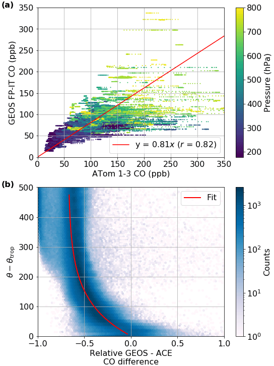
Figure 12 (a) Comparison of colocated ATom-measured and GEOS-FP-IT-forecasted CO mole fractions. GEOS FP-IT CO matched to ATom observations using 4D nearest-neighbor interpolation. The fit is a robust fit using a Tukey biweight function with no intercept, i.e., using the RLM linear model with M = TukeyBiweight() from the Python statsmodels package (Seabold and Perktold, 2010). Only points with pressure < 800 hPa used. (b) Comparison of colocated ACE-FTS and GEOS FP-IT CO data. The x axis is the unitless relative difference, i.e., (GEOS − ACE) $/$ ACE. The y axis is potential temperature relative to the tropopause. The background shading is a 2D histogram of the relative bias between ACE-FTS and GEOS FP-IT CO as a function of θ; the red line is a fit through the mean bias.

3.6.2 Stratosphere

Comparison with ACE-FTS data in the lower stratosphere also demonstrates a low bias that varies with altitude. However, the general structure is consistent as a function of potential temperature relative to the tropopause, as seen in Fig. 12b. This can be represented by an exponential function.

Therefore, the overall CO correction has the form shown in Fig. 13. Below the tropopause, the 1.23 factor derived from ATom is used, while above 380 K (i.e., the stratospheric overworld) the exponential form derived from ACE-FTS is used. In the middleworld, we linearly blend between the two functions in order to provide a smooth transition.

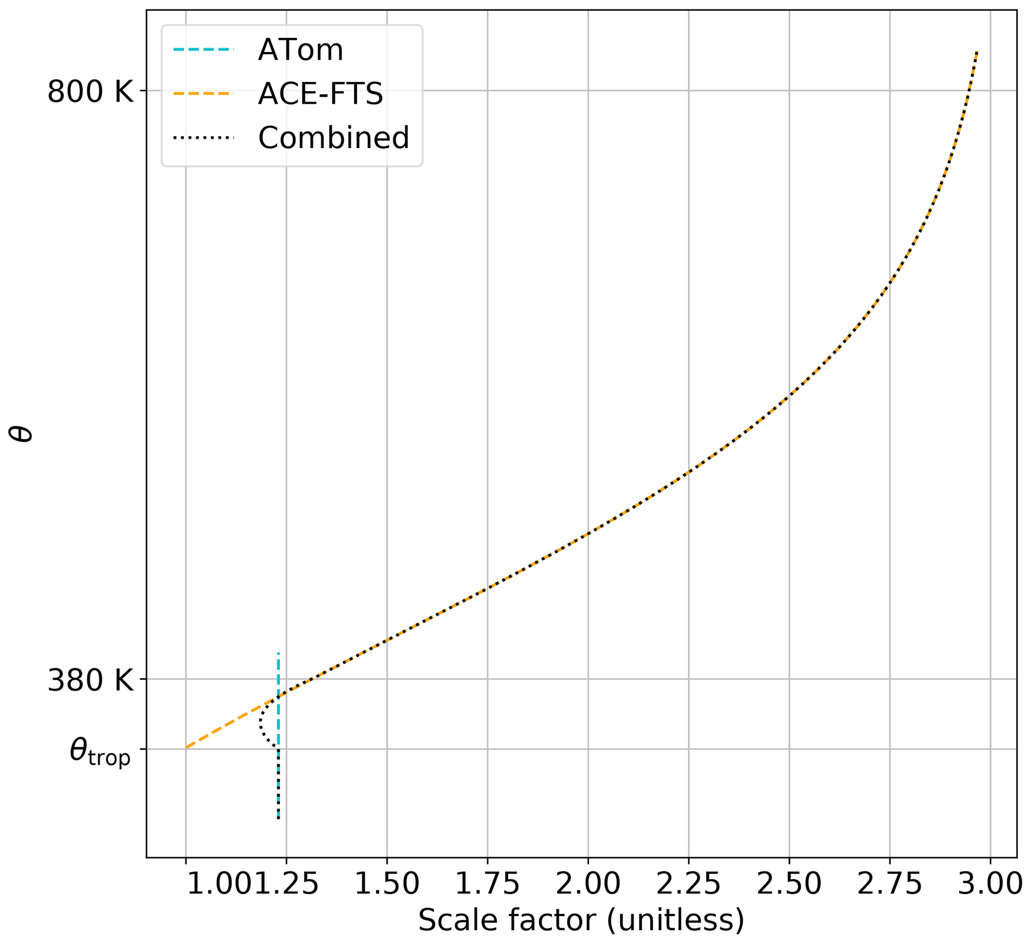
Figure 13 The form of the CO bias correction scaling factor. The blue and red lines show the form derived from ATom and ACE-FTS data, respectively, while the black line shows the blending of these two corrections. Note that the ATom line is extended up to 380 K for reference and does not imply that ATom collected data into the mid-stratosphere.

The second correction required concerns the intrusion of mesospheric CO into the stratosphere. In the mesosphere, very large mixing ratios of CO are produced through photolysis of CO₂. As this descends (especially in the polar vortex), it can lead to very large CO mole fractions at altitudes as low as 40 km. This process is not captured in the GEOS FP-IT product but is represented in the Canadian Middle Atmosphere Model (CMAM), which compares well with ACE-FTS and MLS data (Jin et al., 2009; Kolonjari et al., 2018). Here we use output from a version of CMAM run with dynamics specified (see Sect. 2.2 of Kolonjari et al., 2018, and references therein).

Comparison of GEOS FP-IT with ACE-FTS data shows the mesospheric CO impact beginning around 30 hPa and becoming dominant by 10 hPa. Therefore, we replace the GEOS FP-IT CO with CMAM CO above 10 hPa (i.e., at pressure < 10 hPa) and linearly interpolate from GEOS FP-IT to CMAM in pressure–log space between 30 and 10 hPa. The CMAM CO is drawn from a monthly climatology constructed from the monthly averaged CO DMFs in the 30-year CMAM model run (available at https://climate-modelling.canada.ca/climatemodeldata/cmam/output/CMAM/CMAM30-SD/mon/atmosChem/vmrco/index.shtml, last access: 24 July 2019; Canadian Centre for Climate Modeling and Analysis, 2019). CMAM model data before 2000 are not used in the climatology because there is not a trend present after 2000.

The third and final correction accounts for the mesospheric CO itself. While the priors used in TCCON retrievals have a 70 km ceiling, the CO above that altitude in the CMAM model can comprise up to ∼ 2.5 % of the total column, particularly in the polar regions. To account for this in the prior, we add an equivalent mass of CO to the top level of the priors. This is detailed in Sect. S4 of the Supplement.

3.7 H₂O and HDO

The H₂O profile is computed directly from the GEOS FP-IT specific humidity. The HDO profile is directly computed from the H₂O profile as

$$\begin{array}{}\text{(13)}& c_{\mathrm{HDO}}=c_{{\mathrm{H}}_{\mathrm{2}}\mathrm{O}}\cdot \mathrm{0.14}\cdot \left[\mathrm{8}+{\log }_{\mathrm{10}}\left(c_{{\mathrm{H}}_{\mathrm{2}}\mathrm{O}}\right)\right],\end{array}$$

where $c_{{\mathrm{H}}_{\mathrm{2}}\mathrm{O}}$ and c_HDO are the DMFs of H₂O and HDO, respectively. In the GGG retrieval, the line intensities of isotopologues are multiplied by the isotope abundance. This form therefore does not need to reproduce the abundance of HDO but instead just the decrease in HDO relative to H₂O with altitude due to Rayleigh fractionation (Kuang et al., 2003). While reading the priors, GGG takes the absolute value of the HDO DMF to eliminate negative DMFs resulting from H₂O $<{\mathrm{10}}^{-\mathrm{8}}$. In versions of ginput after 1.1.4, the absolute value of the HDO DMF is output.

4 Use of CO₂ priors for OCO-2 and OCO-3

The Orbiting Carbon Observatory 2 (OCO-2) and OCO-3 retrievals use these CO₂ priors starting in their respective version 10 products. The version 10 products use this algorithm exactly as described above except for one small change: in Eq. (1), l is geographic, rather than effective, latitude. This difference ensures a smooth latitudinal variation in CO₂. Using effective latitude introduced discontinuities near the Equator (Fig. S17a).

The specific structure of the discontinuities in Fig. S17a arises because version 10 of the OCO-2/3 algorithm uses an earlier version of the priors algorithm than GGG2020; in this earlier version, rather than transition between geographic latitude and effective latitude between 20 and 25^∘, effective latitude was used for profiles at all latitudes but disallowed from crossing the Equator (i.e., a profile in the Northern Hemisphere could not have an effective latitude in the Southern Hemisphere and vice versa).

Switching the version 10 priors to use geographic latitude for all soundings trades some ability to capture day-to-day variation in the troposphere for guaranteed spatially smooth priors (Fig. S17b), which is well worth it for nadir-viewing instruments such as OCO-2 and OCO-3. In contrast, for discrete measurement sites such as TCCON, the ability to capture day-to-day variations is preferred.

The OCO-2/3 version 11 priors introduced an additional change to allow more frequent updating of the input in situ data. GGG2020 and OCO-2/3 version 10 use a static file of MLO and SMO data as input that contains monthly averages of flask data prepared by NOAA (Dlugokencky et al., 2019) up through the end of 2018. These records are extended by extrapolation (see Sect. 2) as needed. This has the virtue of simplicity but cannot capture anomalies in the trend of CO₂ such as those caused by El Niños.

The OCO-2/3 version 11 algorithm switched to using hourly in situ data from the continuous trace gas analyzers stationed at MLO and SMO NOAA observatories (Thoning et al., 2021) that has undergone preliminary quality control but not full background selection by NOAA personnel. These hourly in situ data are preprocessed by the priors code to produce monthly averages, allowing the main algorithm to use either monthly flask or hourly in situ data as needed. The preprocessing algorithm is described in Sect. S5 of the Supplement.

5 Validation

5.1 Comparison with aircraft and AirCore observations

To directly validate the GGG2020 priors, we use aircraft data from the NOAA CO₂ GLOBALVIEWplus v5.0 Obspack (Cooperative Global Atmospheric Data Integration Project, 2019; Masarie et al., 2014), NOAA CH₄ GLOBALVIEWplus v2.0 ObsPack (Cooperative Global Atmospheric Data Integration Project, 2020; Masarie et al., 2014), and the Infrastructure for Measurement of the European Carbon Cycle (IMECC) campaign (Geibel et al., 2012), as well as AirCore (Tans, 2009; Karion et al., 2010) profiles from NOAA routine and campaign balloon flights (v20201223, Baier et al., 2021) and selected AirCore balloon flights from FMI/RUG at the Sodankylä, Finland (Kivi and Heikkinen, 2016), TCCON site and CARE-C/LSCE/LMD/IPSL at the Nicosia, Cyprus, TCCON site. Data from tower measurements at Park Falls, WI, USA (Andrews et al., 2014; Desai et al., 2015), the Southern Great Plains Atmospheric Radiation Measurement facility near Lamont, OK, USA, and at the National Institute of Water and Atmospheric Research Ltd. site in Lauder, New Zealand, were used to extend airborne profiles in these locations to the surface as needed. The data used and which gases are provided by each are tabulated in Tables S1 and S2.

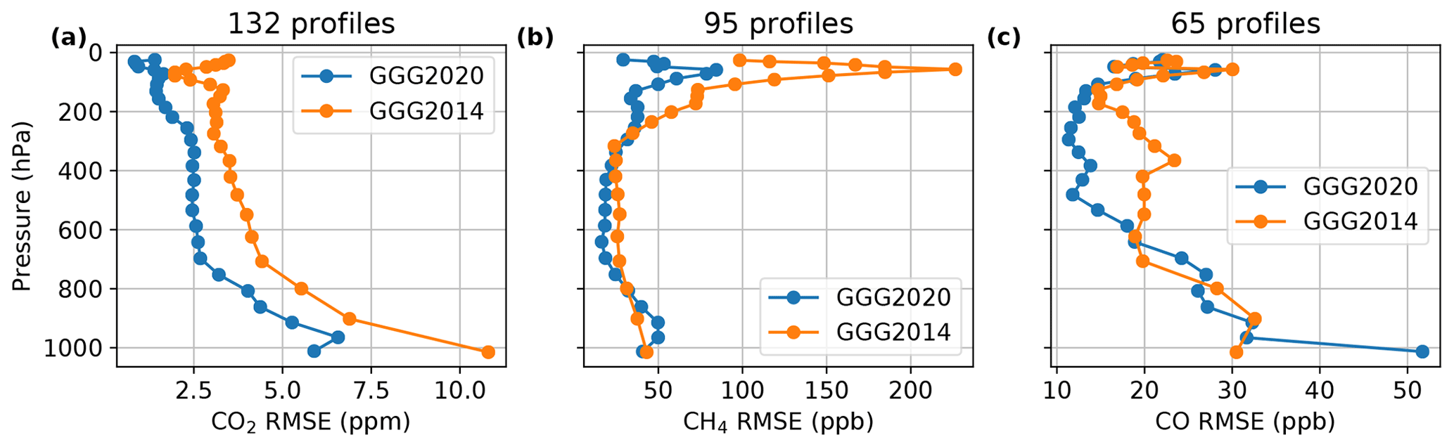
Figure 14 Root-mean-square error (RMSE) of (a) CO₂, (b) CH₄, and (c) CO priors versus combined AirCore and aircraft observations. Data sources are listed in Tables S1 and S2. In each panel, both the GGG2020 and GGG2014 priors' RMSEs are shown. The number of profiles contributing to each panel is printed above the panel. FMI/RUG Sodankylä AirCore data above 20 km altitude are not included due to anomalously high mixing ratios in CO. CO₂ and CH₄ data above 20 km are also excluded for consistency.

Figure 14 shows the root-mean-square error (RMSE) for each vertical level of both the GGG2014 and GGG2020 priors. Mean and individual profile errors are given in Fig. S10. A breakdown of the number of profiles by gas and source is given in Table S4.

For CO₂, the RMSE is noticeably smaller at all altitudes for the GGG2020 priors compared to the GGG2014 priors (Fig. 14a). This results from removing a small but clear negative bias throughout the troposphere arising from an underestimate of the CO₂ secular growth rate in GGG2014. Using the MLO and SMO data eliminates that as a source of uncertainty for profiles before 2019 (2019 is the first year that the MLO and SMO trend is extrapolated for GGG2020 as we chose to use a static file to avoid the complications of updating the input data in a reliable, reproducible manner, as discussed in Sect. 2). In the stratosphere (above 200 hPa), the improved representation of stratosphere dynamics (Sect. 2.3) better captures the gradient of CO₂ in the lower stratosphere, reducing the previous overestimate of lower stratospheric CO₂ in the GGG2014 priors.

The CO₂ RMSE for the GGG2020 priors is still greater near the surface than at higher altitudes. This may be due to the simplified seasonal cycle (Sect. 2.2). Comparing the priors to ATom and HIPPO observations in different seasons (Fig. S8) shows large differences near the Northern Hemisphere surface in spring and summer. As the seasonal cycle has latitudinal dependence, revising its parameterization will require adjustment to the distance function (Eq. 1) and the α and β coefficients (Table 3). This area will be revisited in a future version of the GGG priors.

CH₄ shows a small improvement in RMSE throughout most of the troposphere (Fig. 14b, 800 to 200 hPa). Above 200 hPa, the RMSE shows a greater improvement, again due to the improved representation of stratospheric dynamics. However, near the surface (below 800 hPa) the RMSE increases somewhat in the GGG2020 priors compared to the GGG2014 priors. This increase in RMSE is driven by near-surface CH₄ emissions not accounted for in the priors. Figure 15a shows differences in the CH₄ priors versus AirCore data (which has frequent sampling of areas with high emissions), colored by which TCCON site the prior represents. The bias in CH₄ below 800 hPa is clearly due to underestimated CH₄ in the Lamont, OK, profiles. The Lamont TCCON site is situated near a region of significant oil and natural gas production (Karion et al., 2015), and it thus experiences enhanced CH₄ mole fractions of 100 to 200 ppb near the surface (Fig. S13). Neither the GGG2014 priors nor the GGG2020 priors attempt to account for local anthropogenic emissions. The increase in RMSE near the surface in the GGG2020 priors is due to the removal of a compensating error in assumed vertical gradients – introducing the tropospheric effective latitude (Sect. 2.2.1) accounts for times when Lamont has a profile that varies less with altitude due to the influence of tropical air.

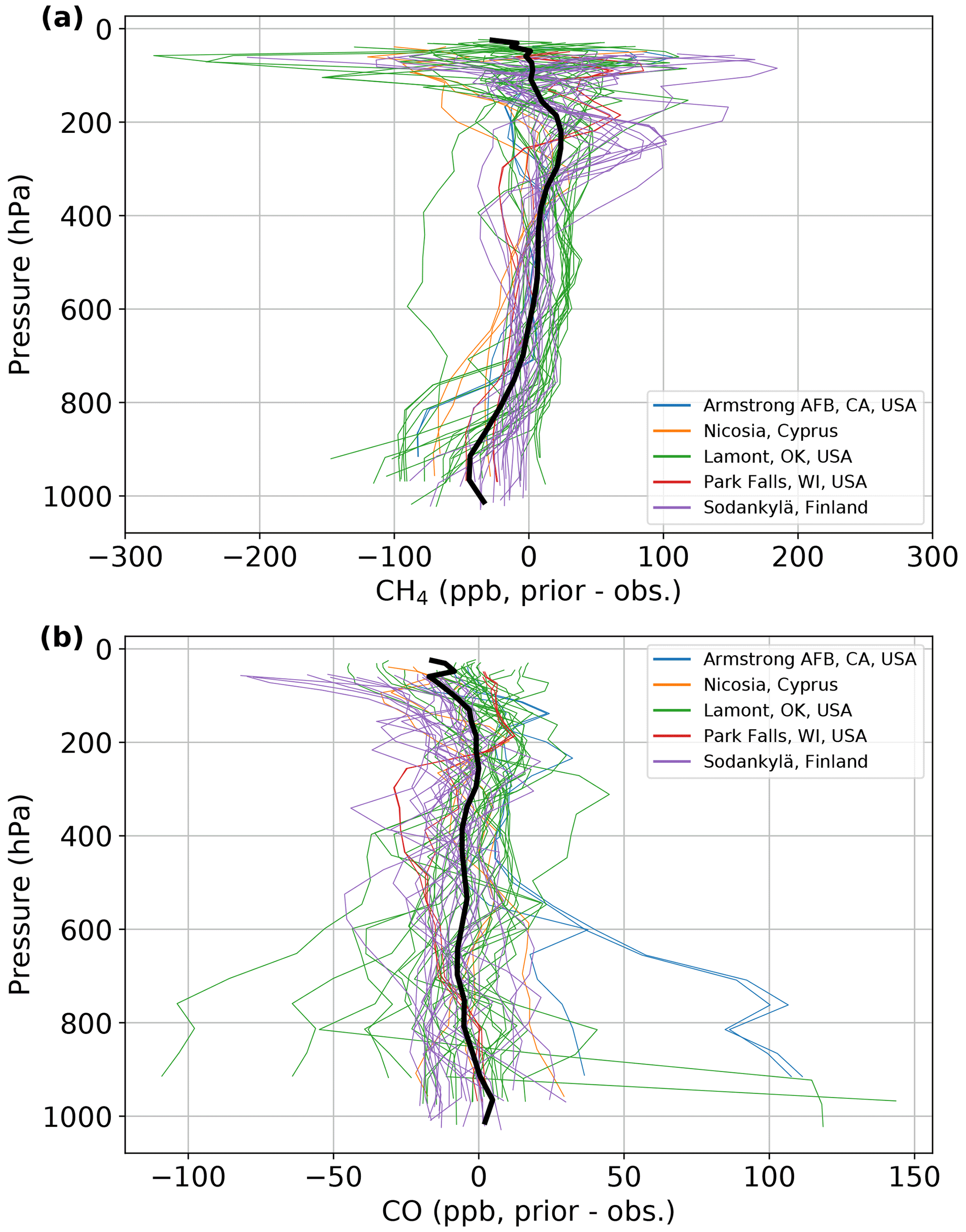
Figure 15 Difference plots for GGG2020 priors versus (a) CH₄ and (b) CO AirCore data. The thinner, colored lines represent differences for individual profiles, and the thick black line indicates the mean difference across all profiles shown. The individual differences are colored by their TCCON site.

The GGG2020 CO priors' RMSE improves throughout the free troposphere (600 to 200 hPa). Unlike CO₂ and CH₄, RMSE is similar between GGG2014 and GGG2020 in the stratosphere (above 200 hPa). Near the surface, the GGG2020 priors' RMSE is ∼ 20 ppb greater than GGG2014. Figure 15b shows that this is driven by overestimated CO at the Armstrong Air Force Base (AFB) TCCON site and both overestimated and underestimated CO at the Lamont TCCON site.

The cause of the overestimates and underestimates in the Lamont profiles is not clear. The GGG2020 CO profiles are based on the CO field in the GEOS FP-IT product (Sect. 3.6). The underestimated CO DMFs could be due to changes in energy economies in the region in recent years (Franklin et al., 2019; Willyard and Schade, 2019). GEOS FP-IT uses 2008 anthropogenic CO emissions for all years after 2008 (Lesley Ott, personal communication, 2019), and thus the CO priors would have no information on changes past 2008.

The overestimated CO at Armstrong AFB is due to its proximity to Los Angeles. CO emissions in Los Angeles have been decreasing (Brioude et al., 2013), a trend not captured in GEOS FP-IT as 2008 emissions are repeated for all years after 2008. Additionally, given that the GEOS FP-IT model resolution is 0.67^∘ × 0.5^∘ (longitude × latitude), that the topography of the Los Angeles Basin is complex, and that Armstrong AFB is only ∼ 0.8^∘ north of Los Angeles, the model is likely not able to capture the full separation of Los Angeles and Armstrong profiles.

Outside of urban or energy-intensive locations, the agreement between the new GGG2020 priors and colocated in situ profiles is much improved. Figure S15 compares RMSEs and mean prior versus in situ differences for CO when Armstrong AFB, Lamont, and Orléans (another near-urban location) are excluded from the comparison. In that case, the RMSE reduces by about a factor of 2 or better at all levels except the surface in the new GGG2020 priors compared to the GGG2014 priors.

We compared CO profiles from the GEOS FP-IT product to the Copernicus Atmospheric Monitoring Service (CAMS) model to see if this issue of overestimated CO is common among models. The results for 2018 through 2022 are shown in Fig. S16. In general, GEOS FP-IT CO is dramatically greater than CAMS CO in Los Angeles (at the Pasadena TCCON site). This is also true at Armstrong AFB but to a lesser extent. In Paris, both models exhibit very high surface CO on some of the sampled days, though this was more frequent in the GEOS FP-IT CO profiles. At Lamont and East Trout Lake, both models had CO DMFs of similar magnitude (even with our factor of 1.23 scaling applied to the GEOS FP-IT data), with the main difference being in vertical distribution. While the factor of 1.23 applied to bring the GEOS FP-IT CO in line with ATom observations (Fig. 12) definitely aggravates the GEOS FP-IT overestimate in urban areas, it improves the mean CO in more remote areas. In the future, drawing CO profiles from a model that better represents urban–rural CO gradients would improve the CO priors but requires an existing model run that also covers the full range of times needed by TCCON (from 2004 on).

Despite the increase in RMSE near the surface, overall the CO priors demonstrate important improvement. The reduction in error in the mid-troposphere will be very beneficial to TCCON retrievals, as the CO averaging kernels increase with altitude up to the tropopause. Therefore, the retrievals are more sensitive to errors in the upper troposphere than the surface. We performed a sensitivity test where we retrieved 1 year of XCO at Armstrong using two sets of priors. We found that the sensitivity of the retrieved XCO to the surface CO in the prior was small, with only a 0.024 ppb change XCO per 1 ppb change in surface prior CO (2.4 %, Fig. S14c).

5.2 Indirect validation through retrievals

We can also evaluate the quality of the priors indirectly using the TCCON retrievals themselves. TCCON uses a scaling retrieval, in which the prior profiles are multiplied by scalar volume mixing ratio scale factors (VSFs) until the optimal match between the forward spectroscopic model and measured spectrum is found. A VSF near 1 usually indicates that the prior profile represented the true atmospheric column abundance well (provided that the forward model spectroscopy is accurate), though it is also possible that compensating errors also yield a VSF near 1. However, given that the direct validation shown in Sect. 5.1 does not show compensating positive and negative biases on average, we expect such compensating errors are unlikely.

Figure 16 shows VSFs for HF and N₂O. Figure 16a shows that the median HF VSF decreased from ∼ 1.25 in GGG2014 to ∼ 0.94 in GGG2020, and the distribution is substantially tighter. HF is found only in the stratosphere (Washenfelder et al., 2003); therefore, this result provides additional evidence that the stratosphere is well modeled by the GGG2020 priors.

Figure 16 Volume mixing ratio (VMR) scale factors (VSFs) of (a) HF and (b) N₂O retrieved using GGG2014 and a preliminary version of GGG2020. The vertical dashed gray line marks a VSF value of 1.

Figure 16b shows that N₂O VSFs moved slightly closer to 1 in GGG2020 with a tighter distribution. N₂O is well mixed in the troposphere with an extremely uniform mixing ratio but varies substantially in the stratosphere due to loss via photolysis. Again, this implies improvement in the stratospheric priors and is a valuable check, as we did not directly validate N₂O against aircraft or AirCore observations due to sparse N₂O profiles over TCCON stations.

Finally, we also consider the interhemispheric bias in CH₄ and N₂O VSFs. For CH₄, Saad et al. (2014) found a ∼ 1 % bias between Northern Hemisphere and Southern Hemisphere CH₄ VSFs using GGG2014 data, and Saad et al. (2016) determined that this was because the GGG2014 priors assumed a smooth DMF profile across the tropopause. In fact, the gradient in the lower stratosphere is driven by stratospheric circulation and CH₄ entering through the tropics (Sect. 2.3). As the priors now correctly account for this, the underlying error driving the interhemispheric bias in tropospheric XCH₄ in Saad et al. (2014) should now be eliminated, and in fact the difference between median CH₄ VSFs between the Northern Hemisphere and Southern Hemisphere has reduced by nearly 50 % (Fig. S11).

For N₂O, the difference between median Northern Hemisphere and Southern Hemisphere VSFs remains nearly the same magnitude (∼ 0.4 %, Fig. S12) but flips with the GGG2020 priors such that the median VSF is now greater in the Southern Hemisphere. Figure S12c compares the surface N₂O DMFs from six NOAA stations against the surface DMFs in the priors for five TCCON sites. While the priors' surface N₂O in the Southern Hemisphere is approximately correct, there is a high bias in the Northern Hemisphere, possibly due to an incorrect assumed tropospheric lifetime (Sect. 3.3) or a need for an additional correction to our distance function (Sect. 2.2) that was not identified during development. This will be corrected in a future version of the TCCON priors.

5.3 Impact on retrieved Xgas values

Figure 17 shows how the bias of the Xgas value retrieved by TCCON relative to in situ profiles changes between using the priors from the previous GGG2014 data version and using the new priors described in this paper. For this comparison, we used only AirCore profiles, as these profiles extend into the lower stratosphere and therefore require the least extension to produce a total column profile suitable for comparison to TCCON. We follow Wunch et al. (2010) in applying TCCON averaging kernels and pressure-weighted integration to the AirCore profiles to produce an in situ Xgas value for comparison to TCCON.

Figure 17 Impact of the new priors on the retrieved TCCON Xgas values compared to coincident AirCore profiles. The x axis shows how the difference between the retrieved TCCON Xgas value and an averaging-kernel-smoothed and integrated in situ profile changes between using the GGG2020 priors described in this paper versus the previous GGG2014 priors. A negative value indicates a reduction in bias compared to in situ with the new priors; the percentage in the title indicates what fraction of the comparisons had reduced bias. The vertical dashed black line marks 0 on the x axis. Each panel is a different TCCON Xgas product; wCO₂ and lCO₂ are experimental TCCON CO₂ products added in GGG2020 that are more sensitive to the upper atmosphere and near surface, respectively, than the standard TCCON CO₂.

For the TCCON CO₂ products, the differences are on the order of 0.05 to 0.1 ppm. Only about half of the comparisons show improvement; this is true for both the standard TCCON CO₂ (Fig. 17, top left) and two experimental CO₂ products introduced in GGG2020 with different vertical sensitivities (wCO₂ and lCO₂, Fig. 17, top middle and top right).

CO worsened on the whole (Fig. 17, bottom right) but by less than 1 ppb. However, this only includes three comparisons at the Armstrong site (most of the comparisons from Fig. 15 are from aircraft profiles, and we only use the AirCore profile here as mentioned above), where the new priors have a known bias (see Sect. 5.1) and none at the Pasadena site (as it is difficult to obtain profiles safely over urban sites), which is more strongly affected by the same issue. Thus, we consider 1 ppb a lower bound on the bias introduced at these sites by the overestimated near-surface CO in the priors.

CH₄ shows the clearest improvement (Fig. 17, bottom left). Almost 80 % of comparisons show reductions in bias relative to the AirCore profiles of up to 13.6 ppb. This likely comes from a combination of the new priors' improved representation of the CH₄ gradient around the tropopause and the general reduction in bias through the free tropopause (Fig. 14).

6 Conclusions

GGG2020 introduces an improved algorithm to generate the prior profiles of CO₂, N₂O, CH₄, HF, CO, and other gases needed for TCCON retrievals. The version 10 and version 11 OCO-2 and OCO-3 retrievals also use these CO₂ profiles. This approach is specifically designed to account for variations in vertical profiles due to synoptic-scale latitudinal motion of air masses. Direct validation against aircraft and AirCore observations shows consistent reduction in error in the free troposphere and lower stratosphere, and indirect validation by examining the magnitude of retrieved TCCON VSFs gives further evidence that the accuracy of the priors in the stratosphere has improved.

The column-average mole fractions retrieved by TCCON shift relative to in situ column averages by up to 0.2 ppm for CO₂, 13 ppb for CH₄, and 1 ppb for CO. For the standard TCCON CO₂, CH₄, and experimental lCO₂ (CO₂ with stronger sensitivity to the surface) products the new priors produce an overall improvement compared to the in situ column averages. The CO and experimental wCO₂ (stronger sensitivity to the upper atmosphere) products compare slightly worse overall to in situ data using the new priors. For CO, this is likely due to overestimated anthropogenic CO emissions in the source model. Finding a way to correct this, either by using a different model run or by applying a geographically varying correction, will be a high priority for the next version of the TCCON priors. The reason for the slight worsening of the wCO₂ retrievals is not yet clear.

An important guiding principle for the GGG2020 priors algorithm was to limit dependence on ongoing measurements or models as much as possible. Doing so means that retrievals using these priors produce data that can be treated as statistically independent with most existing and future measurements and models. Only CO₂, CH₄, and N₂O measurements from the Mauna Loa and American Samoa observatories and CO from the GEOS FP-IT model system are directly ingested, meaning that direct comparisons of TCCON GGG2020 or OCO-2/3 data with these data sources would not be fully independent. As latitudinal gradients from the HIPPO and ATom campaigns and correlations of N₂O, CH₄, and HF from the ACE-FTS instrument are used as well, comparisons between TCCON or OCO-2/3 and HIPPO, ATom, or ACE-FTS data should note that correlations of these specific characteristics (i.e., latitudinal gradients, correlations among N₂O, CH₄, and HF) are correlated by design.

There are still clear areas for improvement. The age of air parameterization used in the troposphere is known to underestimate the age of air compared to SF₆ measurements, and anthropogenic emissions are not accounted for except in the CO priors. Addressing these issues is planned for a future version of GGG; at that time, we will evaluate whether incorporating additional data from measurements or models produces worthwhile improvements in the priors' accuracy. Nevertheless, these new priors represent a significant improvement for the GGG2020 TCCON retrieval.