the Creative Commons Attribution 4.0 License.
the Creative Commons Attribution 4.0 License.
 | 07 Mar 2023
Data quality enhancement for field experiments in atmospheric chemistry via sequential Monte Carlo filters
Patrick Dewald
Clara M. Nussbaumer
Jan Schuladen
John N. Crowley
Jos Lelieveld
Horst Fischer
In this study, we explore the applications and limitations of sequential Monte Carlo (SMC) filters to field experiments in atmospheric chemistry. The proposed algorithm is simple, fast, versatile and returns a complete probability distribution. It combines information from measurements with known system dynamics to decrease the uncertainty of measured variables. The method shows high potential to increase data coverage, precision and even possibilities to infer unmeasured variables. We extend the original SMC algorithm with an activity variable that gates the proposed reactions. This extension makes the algorithm more robust when dynamical processes not considered in the calculation dominate and the information provided via measurements is limited. The activity variable also provides a quantitative measure of the dominant processes. Free parameters of the algorithm and their effect on the SMC result are analyzed. The algorithm reacts very sensitively to the estimated speed of stochastic variation. We provide a scheme to choose this value appropriately. In a simulation study, O3, NO, NO2 and are tested for interpolation and de-noising using measurement data of a field campaign. Generally, the SMC method performs well under most conditions, with some dependence on the particular variable being analyzed.
- Article
(3248 KB) - Full-text XML
-
Supplement
(4835 KB) - BibTeX
- EndNote


Insight into the complex chemical system of the atmosphere is often achieved by conducting coordinated field experiments where an ensemble of trace gases, meteorological variables, physical properties and aerosol compositions are measured that comprehensively characterize the sampled air masses (Hidalgo and Crutzen, 1977; Lelieveld et al., 2018; Wofsy et al., 2018). Field campaigns track variables along a spatiotemporal trajectory and are prone to local and temporal events. These are not resolvable by satellite measurements or chemical–transport models.
Quantitative analysis of data from field campaigns is often hindered by low data quality and insufficient data coverage of all parameters needed at each time step. The latter may result from poor instrumental time resolution, sporadic instrument failures, measurement duty cycles or instrument calibration. Assuming uncorrelated data loss of just 10 % per instrument, a field experiment with 10 different measurement instruments would lose 65 % of simultaneous data.
The reconstruction or enhancement of time steps with lost data or poor data quality is not easily achievable. Linear interpolation and moving average filters act as low pass filters that dampen high-frequency variations of the measured variables. Thus, the main advantage of the field measurement compared to remote sensing is suppressed. The calculation of missing data with photostationary state (PSS) calculations works for many species but introduces a bias as all other processes are disregarded without an estimate of reconstruction error (Ridley et al., 1992). Using the outputs of chemical–transport models as replacements lowers the local and temporal resolution. The latter approach also contradicts the goal of some field campaigns that try to evaluate model predictions (Georgiou et al., 2018).
Sequential Monte Carlo (SMC) methods have become a useful tool in combining prior knowledge of a dynamical system with noisy measurements. Originally applied to trajectory reconstruction (Kitagawa, 1996; Pitt and Shephard, 1999), this method has become a major tool in meteorology for data assimilation to a theoretical model (Bauer et al., 2015; Van Leeuwen et al., 2019). In these fields, the SMC model is applied to enhance the performance of a trusted model with additional information provided by noisy measurements.
Ensemble Monte Carlo methods have been used in relation to atmospheric chemistry measurements where they enabled the estimation of dynamics (Krol et al., 1998), reactions (Berkemeier et al., 2017) or emission sources (Guo et al., 2009; Wawrzynczak et al., 2013). Other novel applications cover enhancements of neural networks and machine learning methods (de Freitas et al., 2001; Ma et al., 2020).
The goal of this work is to explore the SMC method in the enhancement of data quality, data coverage and in the augmentation of data to include unmeasured species in a system of measured atmospheric variables that are connected via known chemical reactions. The focus is shifted from the enhancement of model outputs as in most recent studies (Van Leeuwen et al., 2019) towards data quality enhancement as originally intended (Doucet et al., 2001). Enhanced data quality enables a more comprehensive data analysis of field campaign measurement data. Several applications will be tested on measurements taken in July 2021 at the Taunus Observatory, Kleiner Feldberg, Germany (Dewald et al., 2022). The study will focus on the chemical system of ozone (O3), nitric oxide (NO), nitrogen dioxide (NO2) and the photolysis frequency of NO2 ().
In the following section, the basic theory of the SMC method will be explained. In Sect. 3, the underlying chemistry of the considered system and the measurement techniques used to derive the dataset will be described. In Sect. 4, several experiments using the measured data and the SMC method will be conducted and discussed.
The N-dimensional state vector of a system is defined as at time steps tn (n∈{1…L}). This vector contains all unknown or hidden true values in the system. This state vector evolves partly deterministically according to a transition function fn and partly stochastically by addition of some noise wn. The counterpart of xn is the measurement vector yn∈ℝM that contains all available measurements at time step tn. The elements of the state vector and the measurement vector are connected via an auxiliary function hn that depends on the state vector and measurement noise vn. The functions f and h can also depend on auxiliary parameters u that are considered to be exact.
2.1 Basic procedure
The implementation of an SMC algorithm requires a known conditional probability distribution function (PDF) p(yn|xn) that can be easily calculated and a procedure to sample from the prior PDF (Gordon et al., 1993):
where the distribution contains prior information about the dynamics of the state vector and p(yn|xn) describes the probability of a measurement given a particular realization of the state vector xn. The latter probability distribution encodes the uncertainty of the measurement instruments.
Applying Bayesian theory, the posterior PDF results from the calculation of the expression:
where depends on all previous information. Now the process can be considered Markovian as the dependence on all previous information can be described by direct dependence on the most recent time step only: . This distribution is most likely not a retractable expression (Doucet et al., 2000). An exception is the Kalman filter (Kalman, 1960) that requires the transition function f and the measurement function h to be linear with purely Gaussian-distributed state and measurement noise. These conditions are not met in a system of chemical reactions as the reactions can be highly nonlinear and abundances of molecules follow a probability distribution function (PDF) that is 0 for negative abundances.
The main idea to overcoming this numerical limitation in SMC filters is the approximation of the PDF of xn with a finite number of samples (particles). The PDF of the state vector is approximated by the empirical distribution:
where K represents the number of particles and δ denotes the Dirac measure. If the particles are sampled from the true PDF, the empirical PDF approximates the true PDF for K→∞. Given that the initial particles were sampled according to p(x0), this can be ensured by sequential updating of the particles followed by a bootstrap filter. The particles are updated by application of the transition function to form the prior PDF:
Then, a weight is calculated for each particle that is related to the distance of the particle to the measurement:
The posterior distribution is then approximated by bootstrap resampling (Gordon et al., 1993; Doucet et al., 2000) from the prior particles according to their individual weight q(i). This is implemented by calculation of the cumulative sum of all weights and choosing the kth particle where a uniform random variable u(i) is less or equal to the cumulative sum up to the kth particle:
2.2 Auxiliary particle filter
This approximation assumes that K is large enough. The main challenge of the method is the possibility of the particles to collapse into a single mode (Snyder et al., 2008). It is possible that a single particle carries a weight very close to 1 while all other particles carry weights close to 0. In these cases, the posterior approaches a δ distribution without any statistics. In the literature, there are many approaches to counter this problem, maintaining similar weights for all particles (Van Leeuwen et al., 2019). This is especially important for high-dimensional problems such as data assimilation, as the number of particles has to grow exponentially with the size of the measurement vector M (Snyder et al., 2008). A common approach (Doucet et al., 2000; Van Leeuwen et al., 2019) suggests sampling from a proposal distribution instead of the prior that nudges the particles into the direction of the posterior before applying the bootstrap filter. Pitt and Shephard (1999) described a method they called Auxiliary Particle Filter where they define the proposal PDF as
where μ is a likely draw from the prior PDF. This can be achieved by a simplified version of the transition function fn without a stochastic part. For each particle, an intermediate weight λ(i) is calculated and afterwards R>K samples are drawn from the particles where
The prior is then constructed from this mixture prior analogous to Eq. (4). For the posterior evaluation, the weights (Eq. 5) have to be rescaled by the first stage weights (Eq. 10) to compensate the introduced bias before applying the bootstrap filter (Eq. 7). This method can still lead to weight collapse but increases the statistics and efficiency of the SMC method as the particles of the posterior empirical PDF are less likely to be degenerate by construction (Van Leeuwen et al., 2019). Recently, Fearnhead and Künsch (2018) and Van Leeuwen et al. (2019) reviewed several novel approaches to counter this problem for high-dimensional systems such as weather forecasting; Pulido and van Leeuwen (2019) proposed a particle-flow formalism that completely counters weight collapse (Hu and van Leeuwen, 2021).
These methods will however not be considered in more detail since they are typically dealing with N∼109 and M∼107, while a measurement field campaign lies in the range . Due to the high dimension of the former systems, it is very likely that several measurements differ from the prediction by many standard deviations. As mentioned above, the goal in those cases is to optimize a trusted model with the information provided via noisy measurements. In our case, the centerpiece of the system is the observation. The results from our SMC algorithm should never disagree with the measurements but should rather assist the observations, finding a more precise estimate of a variable that is similar to a weighted average of several measurements.
Further weight-maintaining adaptions to the SMC method can be considered for future applications. For now, weight collapse will be tracked throughout the experiments as a metric. In this study, the following entropy will be considered:
where H is close to its maximum value log (K) or log (R), respectively, when all particles share similar weights. The maximum value is reached if and only if the measurement does not contribute any additional information. The effective dimension R* of a posterior can be approximated by exp (H), where a total collapse to a single particle corresponds to H→0 and . Low entropy is not necessarily a tracer for poor performance of the SMC method but might indicate vast deviations of the actual chemical system from the considered model. An example might be sudden emission of relevant trace gases, changes in wind direction or other local effects.
This study focuses on the interplay between tropospheric O3, NO and NO2. According to Leighton (1961) and Nicolet (1965), the concentrations of these trace gases reach a steady state for a few minutes during the daytime. The relevant reactions are
where Reaction (R3) can be considered fast compared to Reaction (R2). The reaction coefficient is taken from Atkinson et al. (2004). The photolysis frequency varies between ca. 0 at night and several 10−3 s−1. The photostationary state is reached when
Under atmospheric conditions, this photostationary state is additionally affected by peroxy radicals predominantly originating from the oxidation of volatile organic compounds (VOCs) by, e.g., OH or O3. Both hydroperoxy (HO2) and organic peroxy radicals (RO2) convert NO to NO2 (Reactions R4 and R5). In addition, further chemical reactions, direct emission, deposition and transport processes influence this steady state (Crutzen, 1979; Parrish et al., 1986; Ridley et al., 1992):
The coordinated measurements (TO21 campaign) took place in July and August 2021 on the Kleiner Feldberg mountain (826 m, 50∘13′18′′ N, 8∘26′45′′ E), Germany, located in a rural, forested region under anthropogenic influence from several large cities within a radius of ca. 35 km. This site has previously been used for field campaigns and is described in more detail in Crowley et al. (2010) and Sobanski et al. (2016). NO and NO2 were measured via a photolysis–chemiluminescence detector described in Tadic et al. (2020) and Nussbaumer et al. (2021). was calculated from actinic flux measurements by a spectral radiance detector (MetCon GmbH) (Bohn and Lohse, 2017). Ozone was measured by two commercial UV absorption monitors (2B Technologies). Several other trace gases and chemical variables were measured during the campaign that will not be considered in this study. An in-depth discussion of all measurements in this campaign can be found in Dewald et al. (2022). Meteorological data were provided by a weather station of the German Weather Service (DWD) on the summit.
3.1 SMC setup
The setup used in this study is based on the following definition: the state vector x and the measurement vector y are both four-dimensional and encode the mixing ratio of O3, NO and NO2 in units of parts per billion volume (ppbv) and the photolysis frequency in seconds (s). Therefore, the auxiliary function h simplifies to the identity. The transition function f is composed of an initial randomization of each dimension that follows a lognormal distribution and numerical integration of the differential equation resulting from the chemical reactions. The parameters of the distribution are chosen so that the mean and standard deviation are equal to the current value and a given standard deviation σ0, respectively. The choice of a lognormal distribution for chemical systems has been discussed, e.g., in Limpert et al. (2001), and solves the problem of otherwise possible negative values for the abundances. With the scheme proposed here, the lognormal distribution approximates a Gaussian distribution as the standard deviation becomes smaller than the mean. Reactions (R1) and (R2) result in the differential equation:
where kB is Boltzmann's constant that converts the reaction coefficient to units of parts per billion by volume per second (ppbv s−1) at given pressure p and temperature T. These values will be input into the calculation as auxiliary variables for each time step. The parameters p, T and k1 will be set as fixed values and their uncertainties will not be considered. However, any deviations from the true values can be compensated via the initial randomization. The function used to calculate the weights as in Eq. (5) is defined as the product of Gaussian kernels:
where σn,m is constructed by
using the characteristic detection limit DL and precision P for each instrument. In cases of missing measurements, the factor is set to 1. To ensure numerical stability, Eq. (15) in the actual algorithm is replaced by
The model output is constructed from full Bayesian inference to convert the approximate probability distribution to an estimate for the state and an estimate of the error:
3.2 Model extension
In each iteration, the individual particles will evolve towards the photostationary state where Eq. (14) equals 0. This state corresponds to the photostationary state for a given , and j. Particles which are close to the measurement then have high probability to be sampled. If no measurement is available, all particles have an equal chance of being sampled. Therefore, the posterior will shift towards the photostationary state in the unsupervised state. This behavior can cause high biases in combination with low uncertainty on the prediction if no measurements are available and, at the same time, the chemistry is dominated by processes not regarded in the algorithm. During nighttime, the photolysis frequency of NO2 is 0, so other sources of NO, e.g., emissions from soil or plants play a dominant role (Wildt et al., 1997). An example of this effect can be found in the supplement.
Thus, we extend the state vector described in the previous section with an additional variable so that . This variable will be called activity and gates the differential equation according to
Now each particle can be either active or passive if η=1 or 0, respectively. If the chemical reactions incorporated into Eq. (14) dominate the chemistry, it is more likely that active particles survive and vice versa. A small probability pη to switch activity is included into the randomization phase to prevent mode collapse. This way the algorithm can turn chemical processes on and off, whichever is more likely according to the measurements. Additionally, the mean value of η can give insights into the relative importance of the chemical processes incorporated.
Figure 1 shows the diel profile of η for the complete dataset in comparison with the diel average of , along with a box–whisker plot. For low photolysis frequencies, the activity lies close to 0 and sharply increases with higher actinic flux. At j≈0.003 s−1, the median activity rises above 50 % and later saturates at around 90 %. The 10 % and 25 % quantiles suggest a very skewed distribution at noon. This indicates deviations from the PSS calculation due to other processes, e.g., Reaction (R4).

Figure 1(a) Diel profile of photolysis frequency (green) and activity η (blue) averaged for each minute interval. Time is in UTC. (b) Box–whisker plot of activity as a function of photolysis frequency. The markers and dotted line mark the median, boxes range from the 25 % quantile to 75 % quantile, the whiskers mark the 10 % and 90 % quantiles, respectively. The dashed black line marks the transition from passive to active regime η>0.5. A clear nonlinear correlation is visible. Although the correlation is nonlinear, the Pearson correlation coefficient equals 0.67.
3.3 Comparison with constrained box-model calculations
Similar calculations have been conducted using observationally constrained box models (Hens et al., 2014; Crowley et al., 2018; Dewald et al., 2022) in which a selection of measured parameters (e.g., trace gas mixing ratios and photolysis rates) are used as time-dependent inputs for a detailed chemical reaction scheme. Physical effects, e.g., deposition and uptake, can be adjusted to best replicate measured outputs (Dewald et al., 2022). Sensitivity studies can be conducted by a variation of reaction rates and other parameters (Crowley et al., 2018). Typically, these model calculations have runtimes in the order of seconds for a full dataset, dependent on the number of reactions.
From a qualitative perspective, these calculations have some similarities with the SMC method. However, in our case, the choice of appropriate constraints is based on Bayesian theory and the quantitative measurement uncertainty. Sensitivity studies are automatically obtained due to the description of the state as a probability distribution. Unconsidered effects can be compensated via stochastic variability. Also, measurement errors are not directly propagated to the output since the measurement vector is separated from the state vector. In the limit of low constraint uncertainties and full chemical description of the system, the outputs of SMC and box-model calculations converge. In other cases, the latter may be used to prepare a full SMC run, benefiting from its low runtime, and enables detailed chemical investigation of the system (Crowley et al., 2018).
In order to study the effect of the SMC method on time series of chemical systems, several experiments were conducted on the measurement. The capability of the method to interpolate missing data points was tested by artificially discarding data and comparing the reconstruction of the SMC algorithm with the original measurement. The result is evaluated using the mean square error (MSE) and the squared error divided by the standard deviation (χ2):
This will be described in more detail in Sect. 4.1 and 4.2. Another possible application is enhancement of the precision of a measurement within a system. For this test, white noise is added to the observed data. The reconstruction is also analyzed in terms of MSE and χ2. The model is performing well if the MSE is close to the uncertainty of the measurement and χ2 is close to 1. Finally, we discuss the possibility to augment the dataset to include unmeasured variables.
We give a depiction of the algorithm used in Sect. 4.1 and 4.2 in Algorithm 1.
Algorithm 1Auxiliary particle filter in a O3, NO, NO2, , η system.
4.1 Interpolation
The SMC method is tested as an alternative to interpolation of missing data by randomly discarding sections of data with interval size T. This process is repeated for each dimension of the state vector, i.e., each molecule and the photolysis frequency. Then, the missing data are reconstructed.
The algorithm described at the beginning of this section is applied to the whole dataset. Missing data in each dimension are automatically interpolated since the algorithm returns a value for x at all time steps. The uncertainty is given by the standard deviation of the ensemble of particles (Eq. 19). If data are missing in some dimension, the likelihood of the particles is less sparse. This leads to survival of more particles and a higher spread of the posterior. Hence, the standard deviation and the entropy increase. Once measurement data are available again, only data points close to the measurements will be sampled. Entropy and standard deviation decrease again. If the mean of the distribution strongly deviates from the measurement at this point, only a few particles survive and both entropy and standard deviation become very small. The resulting standard deviation underestimates the uncertainty of the model at this point. The requirements for the approximation of the posterior with the finite sample of particles does not hold anymore. Therefore, data points where the entropy is small will be discarded. Since there are effectively less particles left to sample from than samples to be drawn, this threshold is set to
After a low entropy incident, the ensemble may require a few iterations to converge again. Considering this effect and discarding additional points may increase the data accuracy while lowering data coverage. Throughout this analysis, no additional points were discarded. In applications, the number of low entropy events may be reduced using an increased ensemble size which requires a longer runtime.
Figure 2 shows an example plot of NO with random artificial data gaps of 30 min that have been interpolated by the SMC method. Depending on activity, the SMC ensemble mean either tends towards the PSS equilibrium or stays approximately constant, while the ensemble spreads and increases the standard deviation. This spreading happens fast in the beginning of a data gap and slows down afterwards. This might follow the behavior of a sum of normally distributed variables. In this example plot, the spreading speed matches the behavior of the system so that the measurement at the end of a data gap lies within the ±1σ interval.
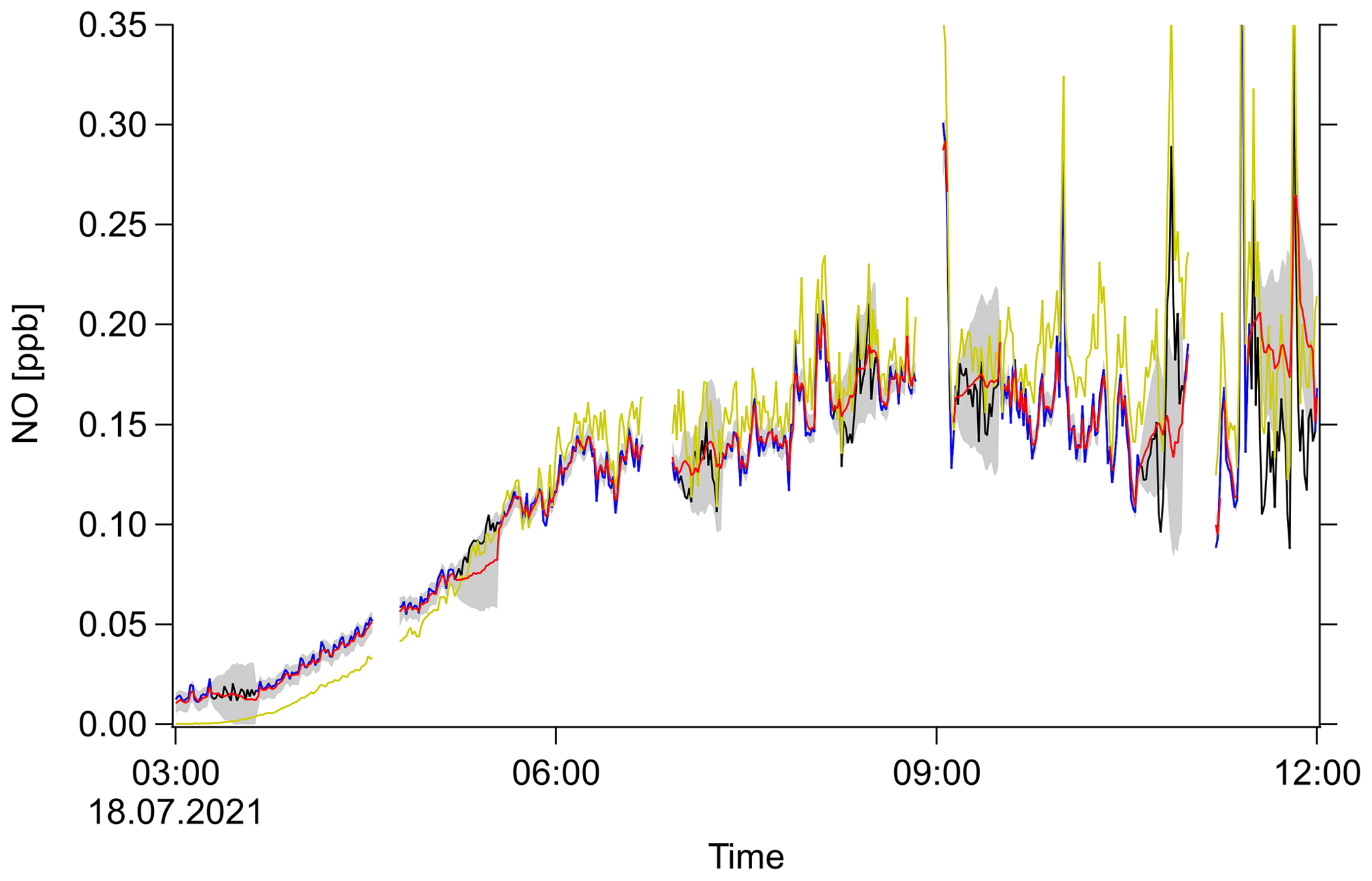
Figure 2Example result of SMC used for interpolation. NO mixing ratio as a function of time (UTC) for an arbitrary day of the field campaign. Original measurement (black), measurement with artificial gaps (blue), PSS calculation (yellow), SMC ensemble mean (red) and ±1σ interval (shaded gray region).
This procedure was repeated for each species and a wide range of data gaps between 1 min and 1 d. The data gaps were shuffled eight times for each setup to achieve better statistics. Figure 3 shows the resulting MSE. For low gap sizes, the MSE stays constant. This constant corresponds to the base deviation of the SMC estimate from the unaltered measurement. This value is expected to be larger than 0, since the model combines the prior knowledge with the measurement and therefore introduces a small bias. We will call this bias the intrinsic model bias.
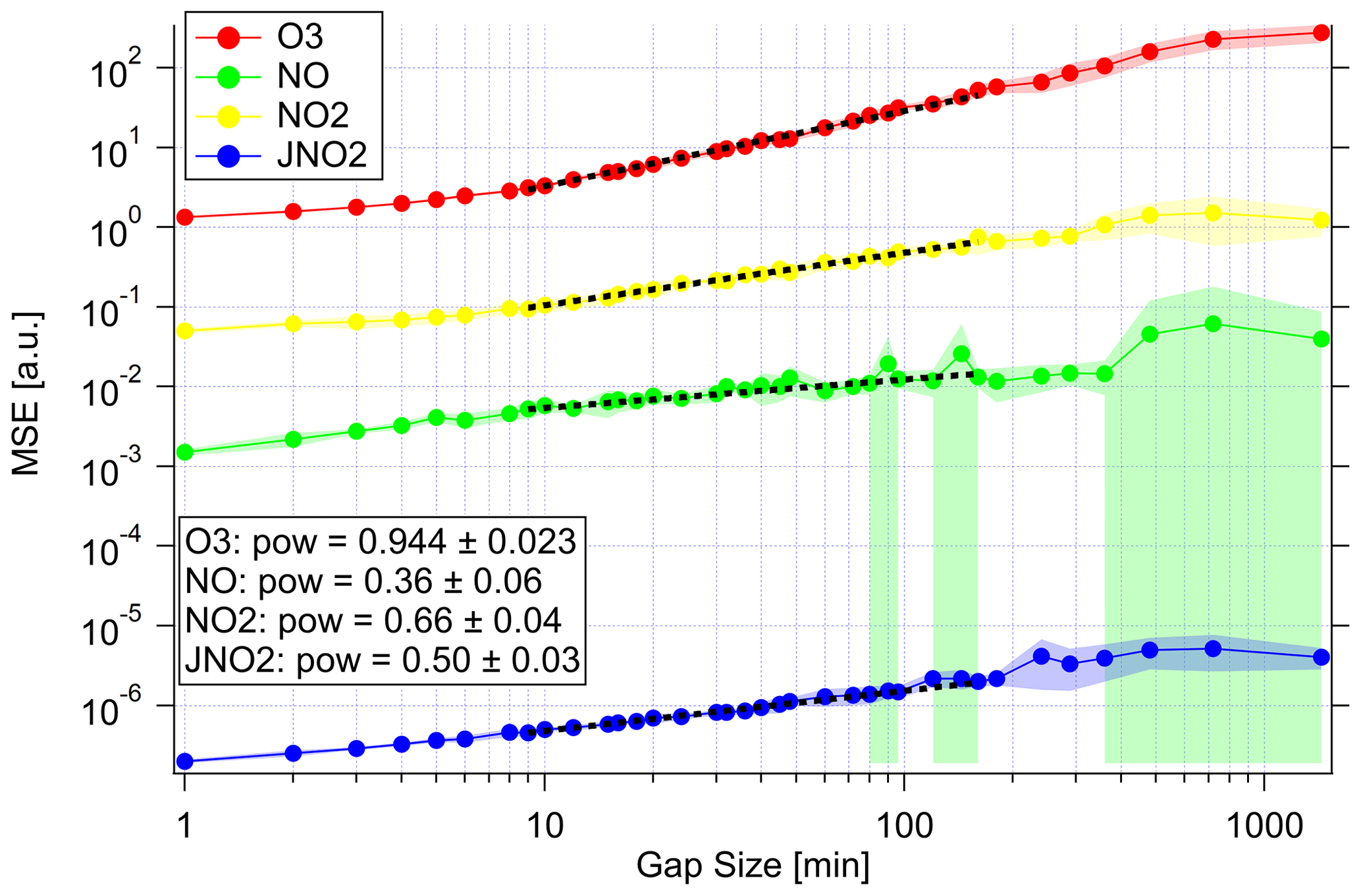
Figure 3MSE of the SMC estimation as a function of artificial data gap size to study the interpolation capabilities. Mean MSE as lines and markers and standard deviation as shaded region for the ensemble of repetitions. The plot shows the results of all variables: ozone (red), NO (green), NO2 (yellow) and (blue). Note that the unit of MSE is arbitrary to fit all variables in one plot. The unit is parts per billion by volume squared (ppbv2) for the MSE of trace gases and inverse seconds squared (s−2) for the MSE of the photolysis frequency. The dashed black lines show power-law fits (y=Axpow) fitted to the intermediate regions. The fit estimate for pow is given in the annotation.
With increasing gap size, the MSE starts to increase. In Fig. 3, it is clearly visible that the slope varies strongly with different variables. This slope corresponds to the power-law coefficient of MSE with larger gap size. In the uninformative case of linear interpolation and Brownian noise, this slope is equal to 1. A lower power-law coefficient indicates an effective contribution of information through the remaining measurements considered. This coefficient is close to 1 for ozone. Therefore, this method is not capable of estimating the course of ozone in cases of instrument failure considering this particular system. This is not a strong limitation since ozone can be measured precisely enough with commercial instruments. However, one should keep this limit in mind in other systems where a species cannot be effectively described by the chemistry of the remaining variables in the system.
At very high gap sizes, the MSE jumps to higher values and the standard deviation also increases. This indicates a higher sensitivity to the particular data gap position. In the limit, the SMC estimate approaches the PSS calculation since no additional information can be provided via measurements. For the variables that can be estimated by PSS reasonably well, the MSE does not increase anymore at the largest gap sizes.
The second performance measure χ2 also increases with larger gap size, but the slope is more sensitive to the actual dynamics of the dataset. If the PSS gives a reasonable estimate of a value but at the same time conflicts with another important process, the SMC estimate follows the PSS and predicts a very low standard deviation. The actual measurement can be multiple standard deviations away from the SMC estimate, thus a high value of χ2 is reached. For NO and , this is most likely the case due to an additional NO source from soil and an additional NO sink via Reaction (R4). Here, χ2 reaches high values before the 2 h mark. A plot can be found in the Supplement.
4.2 Precision enhancement
In this section, the SMC method is applied to artificially noised measurements to test the capability of reconstructing the original signal. The SMC method combines the prior knowledge given by the system dynamics and the precisely measured variables with the remaining information provided by the noisy measurement. If the prior overlaps with the likelihood, the result will be a more precise estimate of the noised variable. If the prior is far away from the measurement due to another process dominating the system, e.g., during the night, the posterior will be close to the likelihood. An example plot is shown in Fig. 4. Here, normally distributed noise is applied to the NO2 measurement. The expected different effects at daytime and nighttime are clearly visible. During the night, the SMC result follows the structure of the measurement while PSS outputs unrealistic values. The noise is reduced only by regularization of the variability through σ0. This effect will be discussed in more detail later. At daytime, the SMC estimate lies between measurement and PSS calculation with a strong tendency towards the photostationary state.

Figure 4Example result of the SMC method used for de-noising: NO2 mixing ratio as a function of time (UTC) for an arbitrary day of the field campaign. Original measurement (black), measurement with artificial noise (blue), PSS calculation (yellow), SMC ensemble mean (red) and ±1σ interval (shaded gray region).
Algorithm 1 is applied again to the noised datasets to obtain values for MSE, χ2 and also the baseline MSE. The latter value in fact equals the square of the noise added. Figure 5 shows the results of this experiment. In all cases, the MSE is constant for low noise. It is dominated by the intrinsic model bias. With increasing noise, the MSE starts to rise once the baseline MSE reaches the intrinsic model bias. At this point though, the MSE increases less steeply than the baseline MSE. Therefore, the additional information provided by the system dynamics successfully decreased the noise. At the same time, the value for χ2 starts to increase. The SMC estimate becomes overly confident as the prediction according to the dynamics can no longer be falsified by measurement accuracy. The MSE and χ2 start to saturate when the limit of extrapolation is reached.
A similar plot showing the resulting values of χ2 is shown in Fig. S3 in the Supplement. The value of χ2 of the photolysis frequency decreases at the beginning until the added noise gets close to the detection limit. Up to this point, the increased uncertainty during the night influences the uncertainty of the SMC estimate which decreases χ2. For O3, the system starts to diverge at high uncertainty. Again, this indicates that ozone cannot be completely reconstructed from the PSS calculation using only the considered molecules. Thus, the application of the method for de-noising is limited when other processes dominate.
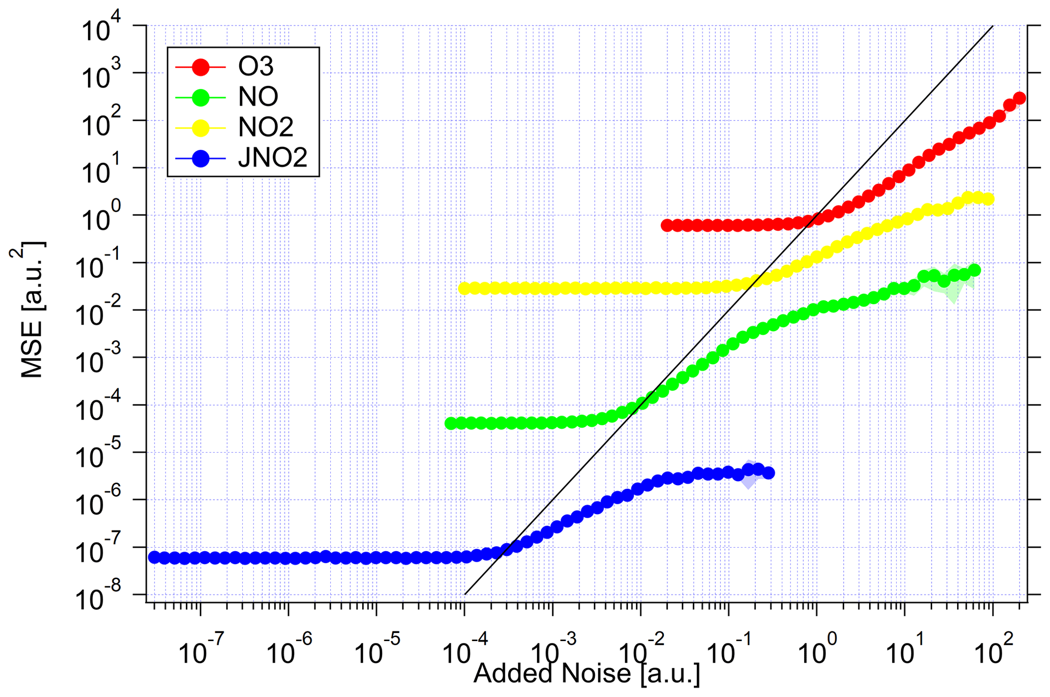
Figure 5MSE of the SMC estimation as a function of artificial noise to study the precision enhancement abilities. The MSE units are represented by lines and markers and the standard deviation by the shaded region for the ensemble of repetitions. The plot shows the results of all variables: ozone (red), NO (green), NO2 (yellow) and (blue). Note that the units of MSE and artificial noise are arbitrary to display all variables in one plot. The unit of the noise is ppbv for the trace gases and inverse seconds (s−1) for the photolysis frequency. The unit of MSE is the square, respectively. The solid black line indicates the baseline MSE (MSE=noise2).
4.3 Extrapolation
The state vector can also be appended with an unmeasured variable. If this variable is strongly coupled to measured variables through the system dynamics, the SMC calculation can give reasonable estimates. This problem can also be interpreted as the limit of infinitely large data gaps or measurements with infinite uncertainty.
Figure 6 shows an example plot of . The SMC result corresponds with the photostationary state calculation, as expected. Additionally, the SMC method is aware of the actual speed of the chemical reactions and is regularized via σ0 with regards to the speed of unconsidered effects. In the example plot, the estimation shows only moderate agreement with the actual measurement. This discrepancy can be explained by other effects interfering with the system, e.g., NO emission from soil during the nighttime or other sinks of NO such as Reactions (R4) and (R5).
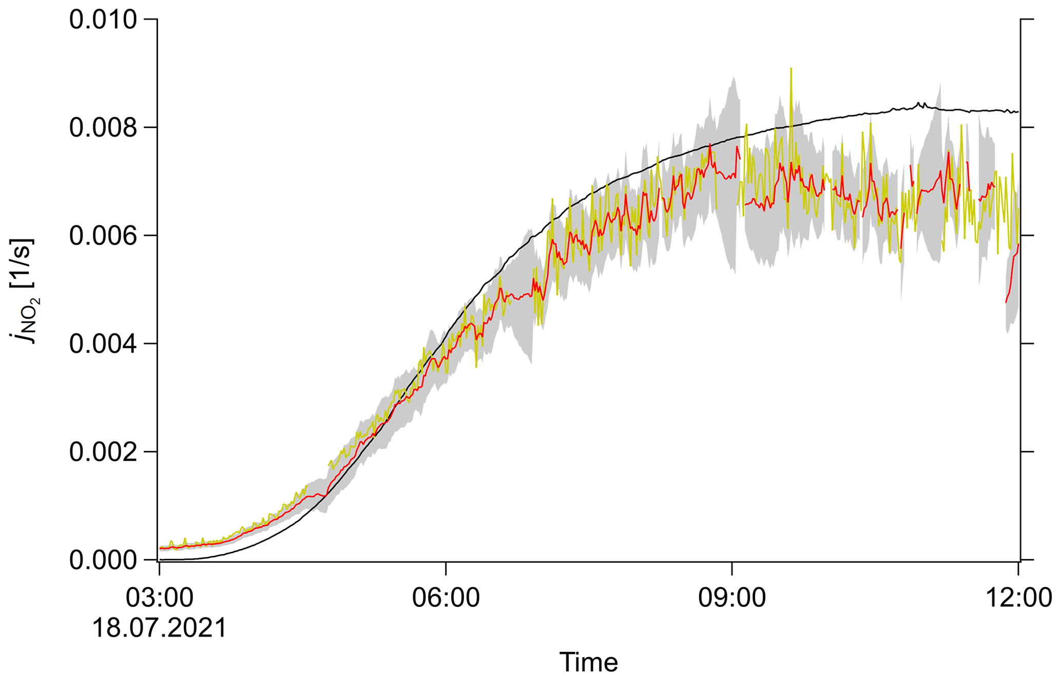
Figure 6Example result of SMC method used for inference. Photolysis frequency j as a function of time (UTC) for an arbitrary day of the field campaign. Original measurement (black), PSS calculation (yellow), SMC ensemble mean (red) and ±1σ interval (shaded grey region).
One has to be careful, however, if multiple unknown variables are coupled. In the case that a small variation in one can be compensated by variation of another variable, the system is singular and will most likely diverge to unrealistic values within a few iterations.
4.4 Free system parameters
The performance of the SMC method can change under variation of important free parameters. The most basic parameter is the measurement error σn,m that relates to the detection limit DL and precision P via Eq. (16). This parameter governs how far particles are allowed to spread from the measurement. An overestimation of this error will bias the algorithm output towards the prior estimate, an underestimation will bias the output towards the measurement. However, σn,m can easily be chosen appropriately if the values of DL and P match the actual performance of the instrument during the measurement.
The switching probability pη has to be tuned for a reasonable performance. If pη is too high, activity is not dominated by inheritance but by random switching. The algorithm will output values similar to the system where activity is set to 1 but with slightly slower dynamics enabled. This also leads to unstable behavior. If pη is too small, it is hard to switch from one state to another. Therefore, the algorithm will become unstable if the environmental conditions switch too fast. Examples are given in the Supplement for the interpolation of the photolysis frequency.
The standard deviation of the prior σ0 has to be chosen carefully. It encodes the expected speed of variation of the system due to stochastic and unconsidered effects. This regularizes the resulting time series to low frequencies. If an appropriate value is chosen for this standard deviation, the algorithm already shows nice de-noising characteristics for each individual variable in x, even if no system dynamic is considered at all. This effect has been reported, e.g., by Riris et al. (1994) and Leleux et al. (2002), for applications of a simple Kalman filter to mixing ratios of trace gases. Therefore, one might encounter seemingly good performance of this algorithm when in fact the result is just dominated by the expected speed of variations.
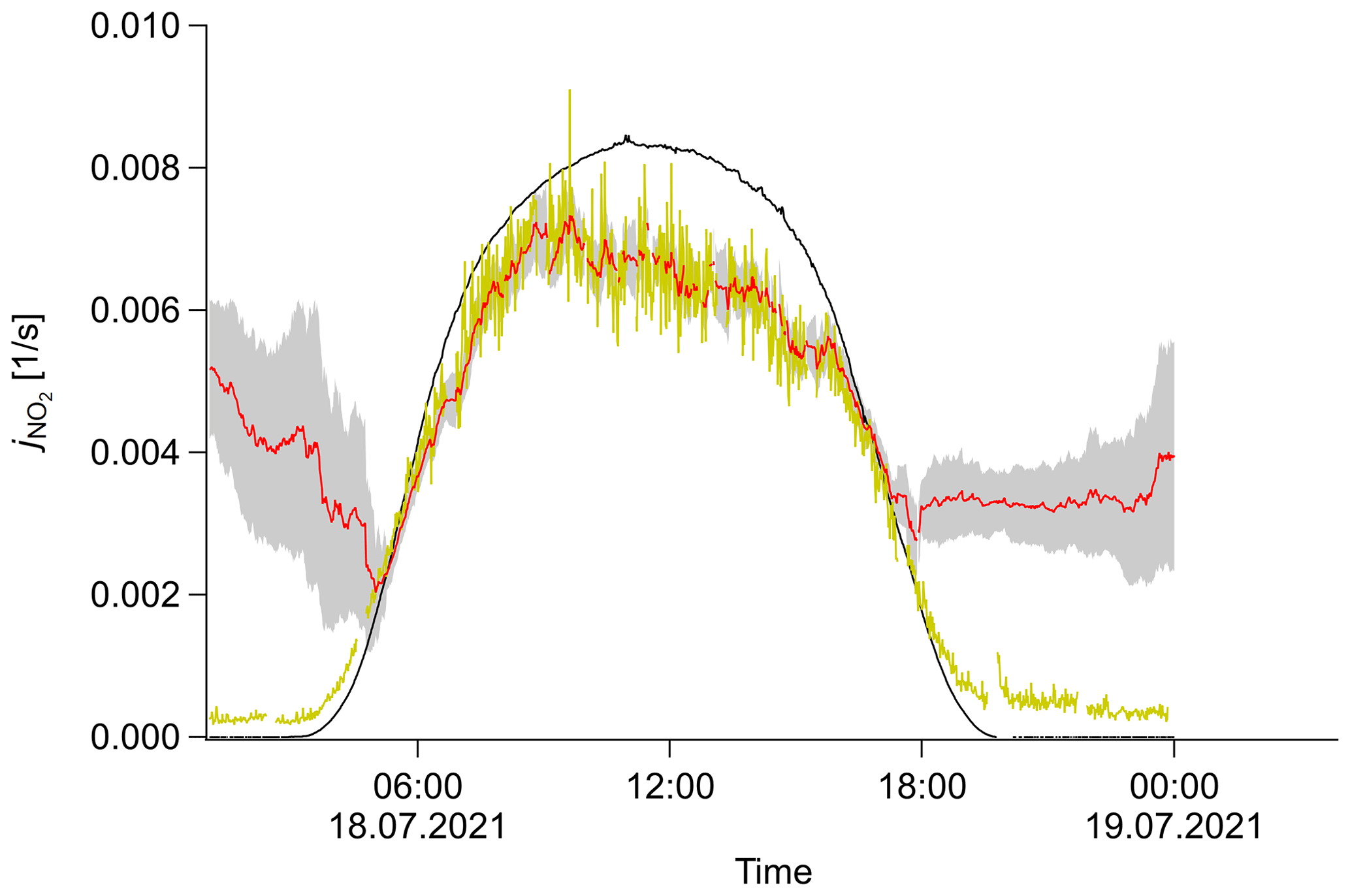
Figure 7Variation of the free parameter σ0 and its exemplary effect on the inference of . σ0,rel is decreased by a factor of 3. Photolysis frequency j as a function of time (UTC) for an arbitrary day of the field campaign. Original measurement (black), PSS calculation (yellow), SMC ensemble mean (red) and ±1σ interval (shaded gray region).
If the value chosen is too small, the system cannot reproduce rapid changes that do not originate from the chosen dynamic. Figure 7 shows an example plot for the photolysis frequency. The system cannot catch up with the speed of sunrise and sunset and decouples from the measurement. If the value is chosen too high, the standard deviation is increased. This can lead to a flattened out probability distribution that effectively reduces the statistics of appropriate particles and therefore can also lead to unstable behavior.
Here, we propose the analysis of the entropy as a measure. If σ0 is too small, the distribution is very condensed and all particles get similar weights. The entropy approaches a constant value. If the value is too high, the distribution spreads out and particles at the edge of the distribution get much lower weights than particles at the center. The entropy decreases with increased σ0. A proper choice of this parameter lies in the transition region from constant entropy to decreasing entropy. An example plot can be found in Fig. S8.
Throughout this study, each σ0 is calculated for each step from a constant and a linear contribution similar to Eq. (16), where σ0,const and σ0,rel are obtained from a linear fit of the measured difference between consecutive samples vs. the measurement itself. This choice falls into the transition region mentioned before. Additional elaborations with regards to this parameter as well as the used σ0 values can be found in the Supplement.
In this study, we demonstrate that the SMC method is a very versatile method that can effectively enhance data quality of atmospheric field measurements. We have shown satisfactory results when applied to data coverage increase, precision enhancement and inference of unmeasured variables. The algorithm is composed of simple steps and only introduces simplified chemical dynamics into a system of measurements. This way, the data quality can be enhanced without precise knowledge of complex reactions and processes such as emission, uptake, deposition or mixing with other air masses. The algorithm automatically detects deviations from the proposed simple dynamics by switching from the active state to the passive state. This ensures stability and gives quantitative insights about the underlying dominant processes. Furthermore, the entropy value encodes the information gained through the measurement and therefore the missing information in the prior estimate.
Along with several benefits over other approaches, we also explored the limitations of this method. Without the model extension by the activity variable η, the algorithm can produce unrealistic estimates when the system dynamics deviate from the proposed reactions. Variables that follow the proposed dynamics quite well and only differ slightly will lead to an underestimation of the standard deviation. Variables that do not follow the proposed dynamics at all do not benefit from the system dynamics but will be regularized with regards to the speed of possible variations. In this case, the algorithm is very sensitive to the proposed values of σ0. This free parameter has to be chosen very carefully. However, a proper value can be chosen by the analysis of observed variations and entropy.
The proposed method should not be seen as a replacement for PSS calculations, box-model calculations, model estimates or actual measurements, but it is an extension to the arsenal of numerical analysis for measurements in atmospheric chemistry. It provides many desirable properties as it is very simple and returns salvageable higher moments of the estimated distribution while requiring a low runtime. A single run with the described setup and the whole 32 d dataset took 18 min of runtime on an 8-core desktop PC.
An open question is the stability of the algorithm when applied to a more complicated system with a higher dimension. Repeating the technical procedure of this study using a higher-dimensional system is restricted by data coverage and data quality in existing datasets. We suggest that many applications of this method for different chemical systems are necessary in the future to fully rate the potential of the SMC method in the analysis of atmospheric chemistry field experimental data.
In general, we emphasize the versatility and high potential of this algorithm. Under the right circumstances, the SMC method can be utilized to enhance data quality and data coverage to allow for a more comprehensive data analysis of field campaign measurement data. However, we suggest conducting similar experiments when applied to a new system of variables. In particular, if the method is applied to a system of precise measurements along with a single imprecise, irregular or nonexistent measurement, the latter variable should be analyzed with regards to interpolation capability, precision enhancement ability and sensitivity to hyper parameters before conclusions can be drawn from the SMC result. These tests could be conducted on modeled data or on a different dataset where the same variables were measured.
Python code is published on Github: https://doi.org/10.5281/zenodo.7677275 (lenroed, 2023).
Data of the TO2021 campaign are available upon request to all scientists agreeing to the data protocol at https://keeper.mpdl.mpg.de/d/f12c1d71d4734a89a6ef/ (last access: 27 June 2022; Crowley et al., 2022).
The supplement related to this article is available online at: https://doi.org/10.5194/amt-16-1167-2023-supplement.
LLR initiated the study, carried out the calculations and analysis and wrote the paper. CMN, PD and JS provided measurement data. JNC and PD contributed to the chemical interpretation of the dataset. JL and HF supervised and consulted the study and defined the goals of this paper.
The contact author has declared that none of the authors has any competing interests.
Publisher’s note: Copernicus Publications remains neutral with regard to jurisdictional claims in published maps and institutional affiliations.
This work was supported by the Max Planck Graduate Center with the Johannes Gutenberg-Universität Mainz (MPGC). We thank Andreas Kürten and Joachim Curtius (Institute for Atmospheric and Environmental Sciences, Goethe University, Frankfurt am Main) for the logistical support and access to the facilities at the Taunus Observatory. We thank the German Weather Service (DWD) for the provision of meteorological data.
The article processing charges for this open-access publication were covered by the Max Planck Society.
This paper was edited by Keding Lu and reviewed by two anonymous referees.
Atkinson, R., Baulch, D. L., Cox, R. A., Crowley, J. N., Hampson, R. F., Hynes, R. G., Jenkin, M. E., Rossi, M. J., and Troe, J.: Evaluated kinetic and photochemical data for atmospheric chemistry: Volume I - gas phase reactions of Ox, HOx, NOx and SOx species, Atmos. Chem. Phys., 4, 1461–1738, https://doi.org/10.5194/acp-4-1461-2004, 2004. a
Bauer, P., Thorpe, A., and Brunet, G.: The quiet revolution of numerical weather prediction, Nature, 525, 47–55, 2015. a
Berkemeier, T., Ammann, M., Krieger, U. K., Peter, T., Spichtinger, P., Pöschl, U., Shiraiwa, M., and Huisman, A. J.: Technical note: Monte Carlo genetic algorithm (MCGA) for model analysis of multiphase chemical kinetics to determine transport and reaction rate coefficients using multiple experimental data sets, Atmos. Chem. Phys., 17, 8021–8029, https://doi.org/10.5194/acp-17-8021-2017, 2017. a
Bohn, B. and Lohse, I.: Calibration and evaluation of CCD spectroradiometers for ground-based and airborne measurements of spectral actinic flux densities, Atmos. Meas. Tech., 10, 3151–3174, https://doi.org/10.5194/amt-10-3151-2017, 2017. a
Crowley, J. N., Schuster, G., Pouvesle, N., Parchatka, U., Fischer, H., Bonn, B., Bingemer, H., and Lelieveld, J.: Nocturnal nitrogen oxides at a rural mountain-site in south-western Germany, Atmos. Chem. Phys., 10, 2795–2812, https://doi.org/10.5194/acp-10-2795-2010, 2010. a
Crowley, J. N., Pouvesle, N., Phillips, G. J., Axinte, R., Fischer, H., Petäjä, T., Nölscher, A., Williams, J., Hens, K., Harder, H., Martinez-Harder, M., Novelli, A., Kubistin, D., Bohn, B., and Lelieveld, J.: Insights into HOx and ROx chemistry in the boreal forest via measurement of peroxyacetic acid, peroxyacetic nitric anhydride (PAN) and hydrogen peroxide, Atmos. Chem. Phys., 18, 13457–13479, https://doi.org/10.5194/acp-18-13457-2018, 2018. a, b, c
Crowley, J. N., Dewald, P., Nussbaumer, C. M., Ringsdorf, A., Edtbauer, A., Schuladen, J., Fischer, H., Williams, J., Röder, L., and Hamryszczak, Z.: Data from TO2021 campaign, Keeper [data set], https://keeper.mpdl.mpg.de/d/f12c1d71d4734a89a6ef/, last access: 27 June 2022. a
Crutzen, P. J.: The role of NO and NO2 in the chemistry of the troposphere and stratosphere, Annu. Rev. Earth Pl. Sc., 7, 443–472, 1979. a
de Freitas, N., Andrieu, C., Hojen-Sorensen, P., Niranjan, M., and Gee, A.: Sequential Monte Carlo Methods for Neural Networks, Springer New York, New York, NY, 359–379, https://doi.org/10.1007/978-1-4757-3437-9_17, 2001. a
Dewald, P., Nussbaumer, C. M., Schuladen, J., Ringsdorf, A., Edtbauer, A., Fischer, H., Williams, J., Lelieveld, J., and Crowley, J. N.: Fate of the nitrate radical at the summit of a semi-rural mountain site in Germany assessed with direct reactivity measurements, Atmos. Chem. Phys., 22, 7051–7069, https://doi.org/10.5194/acp-22-7051-2022, 2022. a, b, c, d
Doucet, A., Godsill, S., and Andrieu, C.: On sequential Monte Carlo sampling methods for Bayesian filtering, Stat. Comput., 10, 197–208, 2000. a, b, c
Doucet, A., de Freitas, N., and Gordon, N.: An Introduction to Sequential Monte Carlo Methods, Springer New York, New York, NY, 3–14, https://doi.org/10.1007/978-1-4757-3437-9_1, 2001. a
Fearnhead, P. and Künsch, H. R.: Particle filters and data assimilation, Annual Review of Statistics and Its Application, 5, 421–449, 2018. a
Georgiou, G. K., Christoudias, T., Proestos, Y., Kushta, J., Hadjinicolaou, P., and Lelieveld, J.: Air quality modelling in the summer over the eastern Mediterranean using WRF-Chem: chemistry and aerosol mechanism intercomparison, Atmos. Chem. Phys., 18, 1555–1571, https://doi.org/10.5194/acp-18-1555-2018, 2018. a
Gordon, N. J., Salmond, D. J., and Smith, A. F.: Novel approach to nonlinear/non-Gaussian Bayesian state estimation, IEE Proc. F, 140, 107–113, 1993. a, b
Guo, S., Yang, R., Zhang, H., Weng, W., and Fan, W.: Source identification for unsteady atmospheric dispersion of hazardous materials using Markov Chain Monte Carlo method, Int. J. Heat Mass Tran., 52, 3955–3962, 2009. a
Hens, K., Novelli, A., Martinez, M., Auld, J., Axinte, R., Bohn, B., Fischer, H., Keronen, P., Kubistin, D., Nölscher, A. C., Oswald, R., Paasonen, P., Petäjä, T., Regelin, E., Sander, R., Sinha, V., Sipilä, M., Taraborrelli, D., Tatum Ernest, C., Williams, J., Lelieveld, J., and Harder, H.: Observation and modelling of HOx radicals in a boreal forest, Atmos. Chem. Phys., 14, 8723–8747, https://doi.org/10.5194/acp-14-8723-2014, 2014. a
Hidalgo, H. and Crutzen, P.: The tropospheric and stratospheric composition perturbed by NOx emissions of high-altitude aircraft, J. Geophys. Res., 82, 5833–5866, 1977. a
Hu, C.-C. and van Leeuwen, P. J.: A particle flow filter for high-dimensional system applications, Q. J. Roy. Meteor. Soc., 147, 2352–2374, 2021. a
Kalman, R. E.: A new approach to linear filtering and prediction problems, J. Basic Eng.-T. ASME, 82, 35–45, 1960. a
Kitagawa, G.: Monte Carlo filter and smoother for non-Gaussian nonlinear state space models, J. Comput. Graph. Stat., 5, 1–25, 1996. a
Krol, M., van Leeuwen, P. J., and Lelieveld, J.: Global OH trend inferred from methylchloroform measurements, J. Geophys. Res.-Atmos., 103, 10697–10711, 1998. a
Leighton, P.: Photochemistry of air pollution, Academic Press, Inc., ISBN: 978-0-12-442250-6, 1961. a
Leleux, D., Claps, R., Chen, W., Tittel, F., and Harman, T.: Applications of Kalman filtering to real-time trace gas concentration measurements, Appl. Phys. B, 74, 85–93, 2002. a
Lelieveld, J., Bourtsoukidis, E., Brühl, C., Fischer, H., Fuchs, H., Harder, H., Hofzumahaus, A., Holland, F., Marno, D., Neumaier, M., Pozzer, A., Schlager, H., Williams, J., Zahn, A., and Ziereis, H.: The South Asian monsoon–pollution pump and purifier, Science, 361, 270–273, 2018. a
lenroed: lenroed/smc-boxmodel: Initial Release, Version v1.0, Zenodo [code], https://doi.org/10.5281/zenodo.7677275, 2023. a
Limpert, E., Stahel, W. A., and Abbt, M.: Log-normal distributions across the sciences: keys and clues: on the charms of statistics, and how mechanical models resembling gambling machines offer a link to a handy way to characterize log-normal distributions, which can provide deeper insight into variability and probability—normal or log-normal: that is the question, BioScience, 51, 341–352, 2001. a
Ma, X., Karkus, P., Hsu, D., and Lee, W. S.: Particle filter recurrent neural networks, in: Proceedings of the AAAI Conference on Artificial Intelligence, 7–12 February 2020, New York Hilton Midtown, New York, New York, USA, 34, 5101–5108, https://doi.org/10.1609/aaai.v34i04.5952, 2020. a
Nicolet, M.: Nitrogen oxides in the chemosphere, J. Geophys. Res., 70, 679–689, 1965. a
Nussbaumer, C. M., Parchatka, U., Tadic, I., Bohn, B., Marno, D., Martinez, M., Rohloff, R., Harder, H., Kluge, F., Pfeilsticker, K., Obersteiner, F., Zöger, M., Doerich, R., Crowley, J. N., Lelieveld, J., and Fischer, H.: Modification of a conventional photolytic converter for improving aircraft measurements of NO2 via chemiluminescence, Atmos. Meas. Tech., 14, 6759–6776, https://doi.org/10.5194/amt-14-6759-2021, 2021. a
Parrish, D., Trainer, M., Williams, E., Fahey, D., Hübler, G., Eubank, C., Liu, S., Murphy, P., Albritton, D., and Fehsenfeld, F.: Measurements of the NOx-O3 photostationary state at Niwot Ridge, Colorado, J. Geophys. Res.-Atmos., 91, 5361–5370, 1986. a
Pitt, M. K. and Shephard, N.: Filtering via simulation: Auxiliary particle filters, J. Am. Stat. Assoc., 94, 590–599, 1999. a, b
Pulido, M. and van Leeuwen, P. J.: Sequential Monte Carlo with kernel embedded mappings: The mapping particle filter, J. Comput. Phys., 396, 400–415, 2019. a
Ridley, B., Madronich, S., Chatfield, R., Walega, J., Shetter, R., Carroll, M., and Montzka, D.: Measurements and model simulations of the photostationary state during the Mauna Loa Observatory Photochemistry Experiment: Implications for radical concentrations and ozone production and loss rates, J. Geophys. Res.-Atmos., 97, 10375–10388, 1992. a, b
Riris, H., Carlisle, C. B., and Warren, R. E.: Kalman filtering of tunable diode laser spectrometer absorbance measurements, Appl. Optics, 33, 5506–5508, 1994. a
Snyder, C., Bengtsson, T., Bickel, P., and Anderson, J.: Obstacles to high-dimensional particle filtering, Mon. Weather Rev., 136, 4629–4640, 2008. a, b
Sobanski, N., Tang, M. J., Thieser, J., Schuster, G., Pöhler, D., Fischer, H., Song, W., Sauvage, C., Williams, J., Fachinger, J., Berkes, F., Hoor, P., Platt, U., Lelieveld, J., and Crowley, J. N.: Chemical and meteorological influences on the lifetime of NO3 at a semi-rural mountain site during PARADE, Atmos. Chem. Phys., 16, 4867–4883, https://doi.org/10.5194/acp-16-4867-2016, 2016. a
Tadic, I., Crowley, J. N., Dienhart, D., Eger, P., Harder, H., Hottmann, B., Martinez, M., Parchatka, U., Paris, J.-D., Pozzer, A., Rohloff, R., Schuladen, J., Shenolikar, J., Tauer, S., Lelieveld, J., and Fischer, H.: Net ozone production and its relationship to nitrogen oxides and volatile organic compounds in the marine boundary layer around the Arabian Peninsula, Atmos. Chem. Phys., 20, 6769–6787, https://doi.org/10.5194/acp-20-6769-2020, 2020. a
Van Leeuwen, P. J., Künsch, H. R., Nerger, L., Potthast, R., and Reich, S.: Particle filters for high-dimensional geoscience applications: A review, Q. J. Roy. Meteor. Soc., 145, 2335–2365, 2019. a, b, c, d, e, f
Wawrzynczak, A., Kopka, P., and Borysiewicz, M.: Sequential Monte Carlo in Bayesian Assessment of Contaminant Source Localization Based on the Sensors Concentration Measurements, in: Parallel Processing and Applied Mathematics, edited by: Wyrzykowski, R., Dongarra, J., Karczewski, K., and Waśniewski, J., Springer Berlin Heidelberg, Berlin, Heidelberg, 407–417, 2014. a
Wildt, J., Kley, D., Rockel, A., Rockel, P., and Segschneider, H.: Emission of NO from several higher plant species, J. Geophys. Res.-Atmos., 102, 5919–5927, 1997. a
Wofsy, S., Afshar, S., Allen, H., Apel, E., Asher, E., Barletta, B., Bent, J., Bian, H., Biggs, B., Blake, D., Blake, N., Bourgeois, I., Brock, C., Brune, W., Budney, J., Bui, T., Butler, A., Campuzano-Jost, P., Chang, C., Chin, M., Commane, R., Correa, G., Crounse, J., Cullis, P. D., Daube, B., Day, D., Dean-Day, J., Dibb, J., DiGangi, J., Diskin, G., Dollner, M., Elkins, J., Erdesz, F., Fiore, A., Flynn, C., Froyd, K., Gesler, D., Hall, S., Hanisco, T., Hannun, R., Hills, A., Hintsa, E., Hoffman, A., Hornbrook, R., Huey, L., Hughes, S., Jimenez, J., Johnson, B., Katich, J., Keeling, R., Kim, M., Kupc, A., Lait, L., Lamarque, J.-F., Liu, J., McKain, K., Mclaughlin, R., Meinardi, S., Miller, D., Montzka, S., Moore, F., Morgan, E., Murphy, D., Murray, L., Nault, B., Neuman, J., Newman, P., Nicely, J., Pan, X., Paplawsky, W., Peischl, J., Prather, M., Price, D., Ray, E., Reeves, J., Richardson, M., Rollins, A., Rosenlof, K., Ryerson, T., Scheuer, E., Schill, G., Schroder, J., Schwarz, J., St.Clair, J., Steenrod, S., Stephens, B., Strode, S., Sweeney, C., Tanner, D., Teng, A., Thames, A., Thompson, C., Ullmann, K., Veres, P., Vieznor, N., Wagner, N., Watt, A., Weber, R., Weinzierl, B., Wennberg, P., Williamson, C., Wilson, J., Wolfe, G., Woods, C., and Zeng, L.: ATom: Merged Atmospheric Chemistry, Trace Gases, and Aerosols, ORNL DAAC [data set], Oak Ridge, Tennessee, USA, https://doi.org/10.3334/ORNLDAAC/1581, 2018. a