the Creative Commons Attribution 4.0 License.
the Creative Commons Attribution 4.0 License.
 | 09 Mar 2023
Climatology of estimated liquid water content and scaling factor for warm clouds using radar–microwave radiometer synergy
Pragya Vishwakarma
Julien Delanoë
Susana Jorquera
Pauline Martinet
Frederic Burnet
Alistair Bell
Jean-Charles Dupont
Cloud radars are capable of providing continuous high-resolution observations of clouds and now offer new capabilities within fog layers thanks to the development of frequency-modulated continuous-wave 95 GHz cloud radars. These observations are related to the microphysical properties of clouds. Power law relations in the form of are generally used to estimate liquid water content (LWC) profiles. The constants a and b from the power law relation vary with the cloud type and cloud characteristics. Due to the variety of such parameterizations, selecting the most appropriate Z–LWC relation for a continuous cloud system is complicated. Additional information such as liquid water path (LWP) from a co-located microwave radiometer (MWR) is used to scale the LWC of the cloud profile. An algorithm for estimating the LWC of fog and warm clouds using 95 GHz cloud radar–microwave radiometer synergy in a variational framework is presented. This paper also aims to propose an algorithm configuration that retrieves the LWC of clouds and fog using radar reflectivity and a climatology of the power law parameters. To do so, variations in the scaling factor ln a (the logarithm of pre-factor a from power law relation) when MWR observations are available are allowed in each cloud profile to build a climatology of the scaling factor ln a that can be used when MWR observations are not available. The algorithm also accounts for attenuation due to cloud droplets. In this algorithm formulation, the measure of uncertainty in the observations, the forward model, and the a priori information of desired variables acts as weights in the retrieved quantities. These uncertainties in the retrieval are analyzed in the sensitivity analysis of the algorithm. The retrieval algorithm is first tested on a synthetic profile for different perturbations in sensitivity parameters. The sensitivity study has shown that this method is susceptible to LWP information because LWP is point information for the whole cloud column. By further investigating the sensitivity analysis of various biases in LWP information, it was found that it is beneficial to incorporate LWP, even if it is biased, rather than not assimilate any LWP.
The algorithm is then implemented in various cloud and fog cases at the SIRTA observatory to estimate LWC and the scaling factor. The scaling factor (ln a) changes for each cloud profile, and the range of ln a is consistent with suggested values in the literature. The validation of such an algorithm is challenging, as we need reference measurements of LWC co-located with the retrieved values. During the SOFOG-3D campaign (southwest of France, October 2019 to March 2020), in situ measurements of LWC were collected in the vicinity of a cloud radar and a microwave radiometer, allowing comparison of retrieved and measured LWC. The comparison demonstrated that the cloud–fog heterogeneity played a key role in the assessment.
The proposed synergistic retrieval algorithm is applied to 39 cloud and fog cases at SIRTA, and the behavior of the scaling factor is studied. This statistical analysis of scaling is carried out to develop a radar-only retrieval method. The climatology revealed that the scaling factor can be linked to the maximum reflectivity of the profile. From climatology, the statistical relations for the scaling factor are proposed for fog and clouds. Thanks to the variational framework, a stand-alone radar version of the algorithm is adapted from the synergistic retrieval algorithm, which incorporates the climatology of the scaling factor as a priori information to estimate the LWC of warm clouds. This method allows the LWC estimation using only radar reflectivity and climatology of the scaling factor.
- Article
(8826 KB) - Full-text XML
- BibTeX
- EndNote


Low-level clouds cover a significant area globally and contribute 60 % of the net radiative forcing in Earth’s radiation budget (Hartmann et al., 1992). Among all the uncertainties in climate sensitivity estimates, the representation of boundary layer clouds has a significant contribution, specifically in the sensitivity of boundary layer clouds to changing surface and boundary layer properties (Bony and Dufresne, 2005). The impact of clouds on climate is further complicated by feedback mechanisms, temperature dependence (Stephens, 2005), and cloud–aerosol interactions (Rosenfeld et al., 2014; Fan et al., 2016). Understanding boundary layer cloud dynamics under changing atmospheric circumstances will help to minimize model uncertainty and climate sensitivity (Bony and Dufresne, 2005). On the other hand, low-visibility phenomena like fog and haze have economic implications in transportation, especially in the aviation sector. Short-range fog forecasts are still inaccurate due to the complexity of fine-scale processes involved in the fog life cycle (Martinet et al., 2020).
Active and passive remote sensing instruments are suitable for long-term cloud observations from space and the ground (Zhu et al., 2017). Such spaceborne (e.g., CloudSat, Stephens et al., 2002; CALIPSO, Winker et al., 2010) and ground-based sensors provide observations of various macro- and microphysical properties of clouds at different temporal and spatial resolution (Illingworth et al., 2007). Earlier studies demonstrated the quantification of cloud microphysical parameters such as effective radius (re) and cloud liquid water content (LWC) using different parameterization with single- or multi-sensor observations as input. The mass of water content in each cubic meter of dry air at a given altitude is defined as LWC, which is an important parameter for understanding the cloud lifetime and evolution processes.
Atlas (1954)Sauvageot and Omar (1987)Fox and Illingworth (1997)Baedi et al. (2000)Wang and Geerts (2003)Krasnov and Russchenberg (2005)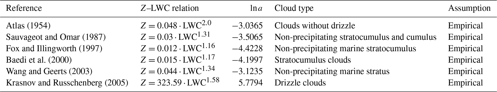
At 95 GHz (3.2 mm), the Rayleigh regime is still valid as the radar wavelength is nearly 2 orders of magnitude larger than the observed cloud droplet size, which is invariably less than 50 µm (Miles et al., 2000). The cloud droplets larger than this size have appreciable terminal velocity, fall out of the cloud, and are termed drizzle droplets. Therefore, radar reflectivity can be considered proportional to the sixth moment of the droplet spectrum, and LWC is proportional to the third moment of the droplet spectrum. However, Mie scattering becomes significant at larger sizes, such as drizzle droplets. An empirical approach of estimating LWC using the radar reflectivity factor by assuming the shape of droplet size distributions (DSDs) is demonstrated in the literature. Z–LWC relationships derived using in-situ-measured droplet spectra collected from a research aircraft are proposed in Atlas (1954), Sauvageot and Omar (1987), and Fox and Illingworth (1997). Table 1 shows details of empirical relations between the radar reflectivity factor Z and the LWC from the literature for a given cloud type. Typically, radar reflectivity Z and cloud liquid water content (LWC) are related to a power law equation given as
where a and b are constant coefficients. If Z is known, LWC can be estimated provided the values of constants a and b are correct for the given cloud type.
LWC calculated using any Z–LWC relationships listed in Table 1 depends strongly on cloud microphysics, which varies significantly with changing ambient conditions. Due to the inherent heterogeneity of cloud droplet spectra, it is challenging to establish a universal Z–LWC relationship as the value of coefficient a varies from 0.012 for marine stratocumulus clouds (Fox and Illingworth, 1997) to 323.59 for drizzling clouds (Krasnov and Russchenberg, 2005), and the exponent b varies from 1 to 2. As mentioned, the empirical approach is also based on certain approximations in DSDs, which widely vary within the cloud and among different cloud systems. Thus, a small variation in larger droplet size strongly influences both Z and LWC, which leads to high uncertainties in estimated LWC profile (Löhnert et al., 2001). Since the cloud droplet size changes significantly within the cloud structure, the retrieval of LWC using only Z information will not be accurate even if the most appropriate empirical relation for the cloud type is used.
To reduce the uncertainties due to unknown droplet spectra, a synergy of two or more active and passive sensors providing additional cloud information with sophisticated retrieval techniques has been used in several studies in the past few decades. Some studies demonstrated the applicability of a dual-wavelength radar system, which uses signals from the Ka–W-band (Hogan et al., 2005) and S–Ka-band (Ellis and Vivekanandan, 2011) to calculate liquid water profile. Frisch et al. (1995, 1998) used total integrated liquid water path (LWP) measured by a microwave radiometer with cloud radar together. LWP is defined as follows:
where dr is the range resolution in meters if LWP is in grams per square meter, and LWC is in grams per cubic meter. This radar–radiometer combination constrained the retrieved LWC exactly to the observed LWP. Further, Ovtchinnikov and Kogan (2000) used simulated cloud data to conclude that the combination of radar reflectivity with liquid water path from a microwave radiometer can significantly increase the accuracy and the robustness of the retrieval. Thereafter, Löhnert et al. (2001) explained a similar approach of using LWP derived using brightness temperature (Tb) from a passive microwave radiometer, radar reflectivity profile from a 95 GHz cloud radar, and cloud model statistics to derive LWC profiles. The limitation of this approach is that the accuracy of the LWC profile is reduced in the presence of drizzle. This is because a few drizzle droplets dominate the reflectivity without contributing much to LWC. In the case of drizzle in the cloud profile, lidar ceilometers are used to determine the actual cloud base height because lidar ceilometers are more sensitive to small cloud droplets than cloud radars. O'Connor et al. (2005) calculated the drop size, liquid water content, and liquid water flux of drizzle using the synergy of cloud radar and backscattering information from lidar. This technique was applied to the drizzle below the cloud base, as the lidar beam is strongly attenuated when it penetrates the cloud. To improve the quality of LWC retrievals in clouds and drizzle, Löhnert et al. (2008) implements a target classification scheme using certain thresholds determined by radar reflectivity and ceilometer extinction profile. Some LWC profile retrievals in the literature are applicable to both precipitating and non-precipitating clouds, although they may have their own set of limitations. Historically, difficulties with fog retrievals were due to the cloud radar blind zone, which can now be minimized with frequency-modulated continuous-wave (FMCW) radars.
The main goal of this study is to learn from the synergistic retrieval and utilize that knowledge to direct the retrieval when synergy is not possible. The instrumentation used in this paper is described in Sect. 2, and the retrieval methodology to develop climatology is explained in Sect. 3. Section 4 elaborates the sensitivity analysis of the retrieval algorithm using a synthetic profile, and the validation of retrieval with in situ measurements is discussed in Sect. 5. After evaluating the performance of the retrieval algorithm, Sect. 6 focuses on the derivation of the climatology of the retrieved parameters, and finally, the BASTA stand-alone retrieval using climatology is discussed in Sect. 7.
Observations for this study are collected from a 95 GHz cloud radar and a microwave radiometer, which are co-located in two different locations. The longest observation period, between November 2018 and May 2019, which corresponds to the meteorological conditions of interest including a relatively higher concentration of fog and cloudy days, is from SIRTA (Haeffelin et al., 2005, Site Instrumental de Recherche par Télédétection Atmosphérique). SIRTA is a multi-instrumental atmospheric research laboratory located in Palaiseau (49∘ N, 2∘ E), 20 km south of Paris (France), in a semi-urban environment that is 160 m above sea level. The observatory brings together several advanced active and passive remote sensing instruments to study the dynamic and radiative processes of the atmosphere recorded since 2002 (Haeffelin et al., 2005). The climatology of liquid cloud retrievals is derived using the observations from SIRTA. Simulations using the French convective-scale AROME model (Seity et al., 2011; Brousseau et al., 2016) for SIRTA are used for sensitivity analysis of the algorithm.
The second site is located in the southwest of France; measurements were collected during the SOFOG-3D (SOuth west FOGs 3D experiment for processes study) field experiment between October 2019 and March 2020. This field experiment was conducted to advance the understanding of fog processes by exploring both horizontal and vertical variability in fog layers. The super-site is located in the Saint-Symphorien commune of France and is centered at 44∘24′44.5′′ N, 0∘35′51.5′′ W, covering a circular surface of 5 km radius around this point. The territory is part of a farm named Domaine de la Grande Téchoueyre, which is 69 m above sea level, and this site was chosen due to its fog occurrence statistics. Additionally, various measurements of fog properties were collected with innovative sensors including in situ and remote sensing networks across a 300×200 km domain around the super-site. In situ measurements collected during this campaign are used to validate the LWC retrieval algorithm in fog conditions. The next part goes into detail about the specifications of instrumentation used in this study.
2.1 BASTA cloud radar at SIRTA and SOFOG-3D
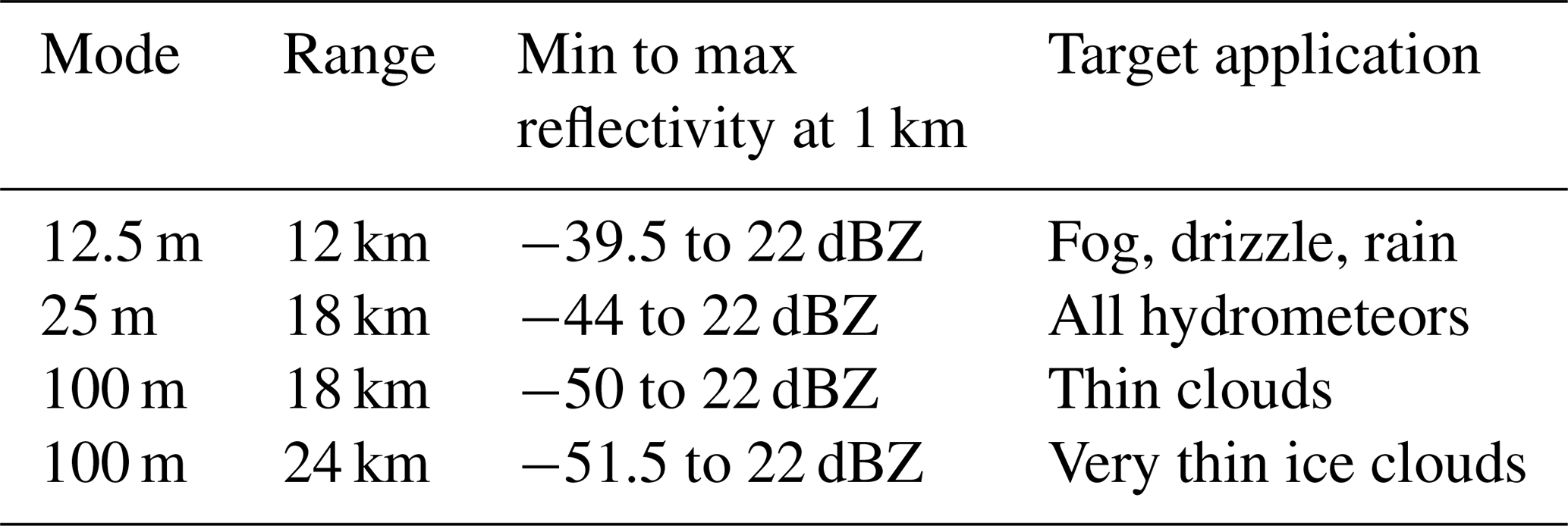
A vertically pointing 95 GHz cloud radar called BASTA (Delanoë et al., 2016) is operating at SIRTA to record the time–height structure of clouds, fog, and light precipitation. BASTA was developed at LATMOS (Laboratoire Atmosphères, Observations Spatiales), and it has been operational at the SIRTA observatory since 2011. This Doppler cloud radar uses the frequency-modulated continuous-wave (FMCW) technique rather than pulses, making it less expensive than traditional cloud radars. It measures radar reflectivity and Doppler velocity of the atmospheric targets at four different range resolution modes depending on the specific application.
In particular, the 12.5 m vertical resolution mode is dedicated to fog and low clouds and is limited to 12 km range height with a minimum range of 40 m. This radar is calibrated using the approach proposed by Toledo et al. (2020) based on corner reflectors. Another product developed by combining three modes providing optimized radar reflectivity, velocity, and mask indicating the valid signal from noise is also developed. This level 2 (L2 here onwards) processing is a new vertical grid derived by combining several modes (vertical and temporal resolution) at the same time resolution in order to make the most of each mode. Table 2 includes information on the various BASTA radar modes, associated vertical ranges, minimum and maximum reflectivity, and target application. The data from the highest range resolution are gridded, while the values from the lower-resolution range are distributed using the closest value. Due to their higher sensitivity, the highest-range-resolution data are utilized, and background noise is eliminated.
In this study, 39 cloud cases with the L2 product of BASTA measurements at the SIRTA location are used. During the SOFOG-3D field experiment, the vertically pointing BASTA radar was deployed in a fog-prone region to acquire high-resolution observations of the fog's characteristics. The L2 product of BASTA observations is used to evaluate the performance of the algorithm for retrieving the LWC of low-level fog. Due to the coupling of the radar antenna, the minimum detectable range was 40 m above the ground for the L2 product.
2.2 HATPRO microwave radiometer at SIRTA and SOFOG-3D
A 14-channel HATPRO (Humidity And Temperature Profiler) microwave radiometer (MWR) manufactured by Radiometer Physics GmbH (RPG) is operational at the SIRTA observatory. The HATPRO MWR is a passive instrument, converting the naturally emitted downwelling radiative energy emitted from the atmosphere within two spectral bands with seven channels each: the first one focuses on the water vapor absorption band (22.24–31 GHz), while the second one is centered on the 60 GHz oxygen complex band (51–59 GHz). Through the use of calibration coefficients, detected intensities are then directly converted into brightness temperatures. A retrieval technique is then needed to convert the brightness temperature spectra into vertical profiles of temperature, humidity, liquid water path. MWRs are sensitive to the total liquid water content in the cloud column (Ware et al., 2002). In general, statistical methods (linear or quadratic regressions or neural networks) trained from simulated MWR observations from a database of radiosoundings or model analyses are used (Cimini et al., 2006). Optimal-estimation retrievals combining an a priori estimate of the atmospheric state with observations through an iterative process can also be used (Martinet et al., 2020). In this study, LWP retrievals based on MWR observations have been retrieved through quadratic regressions trained from a database of radiosoundings for SIRTA, while for SOFOG3D, neural networks trained from AROME short-term-forecasts have been used. Humidity profiles can be retrieved with a limited vertical resolution due to the smoother weighting functions for K-band channels. Temperature profiles show a better vertical resolution, which can be improved through the use of different elevation angles (generally from 90 to 5.4∘ above the ground). A detailed description of the SOFOG3D MWR network and the retrieval data processing is available in Martinet et al. (2023).
For a column containing a single liquid layer, MWR provides the LWP for the cloud layer. The LWP measurements of the column are unaffected by ice clouds above liquid clouds. The time resolution of LWP measurements used in this study is 1 s, with brief interruptions due to boundary layer scans. The missing measurements during boundary layer scans are interpolated to the BASTA observation frequency, which is 0.333 s. The uncertainty in the MWR for LWP is expected to range between 10 and 20 g m−2 (Crewell and Löhnert, 2003; Marke et al., 2016), particularly dependent on the absolute calibration errors in MWR and uncertainties in retrieval algorithms. This uncertainty is also due to uncertainty in the microwave radiative transfer model.
2.3 Cloud droplet probe (CDP) on the tethered balloon during SOFOG-3D experiment
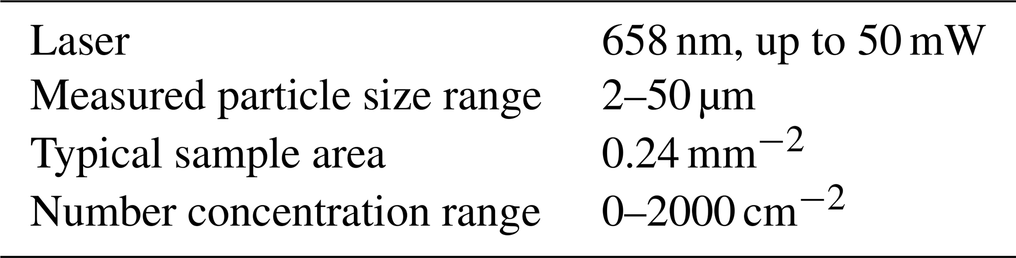
The tethered balloon mounted with an in situ sensor called a cloud droplet probe (CDP) is designed to measure cloud droplet size distribution from 2 to 50 µm. The CDP probe housing contains the forward-scatter optical system, which includes a laser heating circuit, photodetectors, and analog signal conditioning, and an appropriate data system can also calculate various other parameters, including particle concentrations, effective diameter (ED), median volume diameter (MVD), and liquid water content (LWC) (Lance et al., 2010). This instrument is designed and commercialized by Droplet Measurement Technologies, and the specifications are given in Table 3. The sampling rate of CDP was 10 s and had 50 size bins each with 1 µm resolution during the SOFOG-3D campaign.
Table 3Specifications of the in situ cloud droplet probe mounted on a tethered balloon.
The objective of the algorithm is to retrieve LWC using radar reflectivity measurements and LWP derived from MWR when the latter is available. The integrated liquid water content in the cloud column constrains the vertical profile of LWC, which is strongly related to the reflectivity profile. There are several methodologies for modeling such algorithms, including analytical methods, machine learning techniques, and others. The technique proposed in this paper is framed within the context of optimal-estimation theory (Rodgers, 2000). This approach combines a priori information and uncertainties in the observations and the way we represent them and is easily expandable to accommodate additional information from multiple instruments. This retrieval method must be able to combine active and passive remote sensing instruments to derive the most possible accurate climatology of liquid cloud properties and also work when only radar observations are available (i.e., stand-alone version). This must be achieved using a common framework. Such a technique has been widely applied in previous studies (Löhnert et al., 2001; Hogan, 2007; Delanoë and Hogan, 2008). Synergistic retrieval combining radar and a microwave radiometer in order to estimate liquid cloud properties has already been proposed by Löhnert et al. (2001). In their approach, they directly assimilate brightness temperature (Tb) and humidity profiles from the microwave radiometer. The method presented here aims at providing more flexibility when the microwave is not available. Therefore, we do not directly assimilate brightness temperatures, but the microwave radiometer product (LWP) and the associated uncertainties are taken into account. In stand-alone mode, when only radar observations are available, our method relies on a priori knowledge of liquid cloud properties and their link with radar measurements. This a priori information will be built using climatology derived when the radar and the microwave radiometer are simultaneously available.
To account for the large dynamic range of the observations within a profile, this algorithm uses the logarithm of the state variables and measured quantities, which also prevent the unrealistic retrieval of negative values. Therefore, the linear relation between Z and LWC in log space in the form of , where ln a represents the intercept, and b is the gradient of the line, can be written as
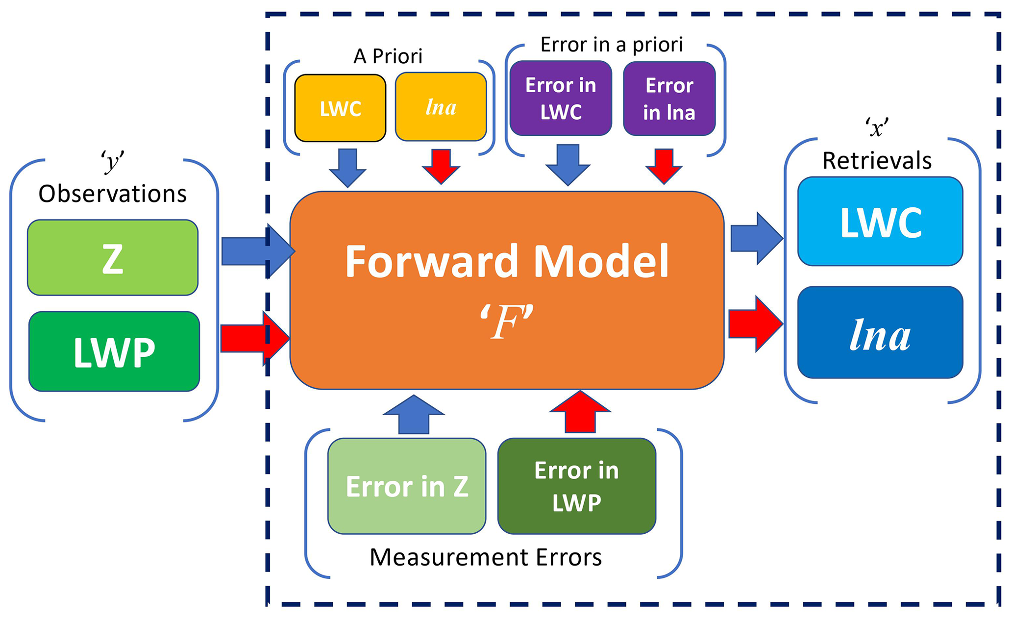
The logarithm of a priori coefficient a is referred to as the scaling factor, and the logarithm also enables visualization of the wide range of a. Figure 1 illustrates how the input parameters (Z and LWP) are used to retrieve the output variables (LWC and ln a). Although the observation vector y may not incorporate LWP when it is unavailable, by adding the LWP in the observation with Z, the forward model allows retrieval of ln a in addition to LWC.
3.1 Optimal estimation and the configuration of state and observation vectors
The optimal estimation (Rodgers, 2000) is a retrieval approach in which the measured quantities are related to unknown atmospheric parameters using a forward model. If “y” is the measurement, and “x” is the unknown parameter, then the forward model “F” and errors “ϵ” can be mathematically written as
where error due to measurements and the forward model are accounted for in ϵ. The forward model is a mathematical description of the atmosphere as a function of the measurements and the atmospheric states. The retrieval starts with the “first guess” (which can be a priori) of the states, and the forward model is then applied to simulate the values of measurements. The states are updated until the simulated and measured quantities are close enough, and convergence is achieved. To sum up, this technique allows the estimation of the atmospheric state, which is physically consistent with the specified errors.
In the optimal-estimation method, minimization of the cost function leads to the iterative solution. Convergence is assessed at each iteration using the following variable to estimate the closeness of the observations with the model:
where “i” is the iteration number, and J is called the cost function. For every iteration, G examines the absolute gradient of the cost function and achieves convergence when the difference between two successive cost functions is negligible. In this scenario, the retrieval converges when G is of the order of 10−7, which indicates that the additional iteration does not add a prominent change in the retrievals.
The state vector “X” is the vector of unknowns and must contain all the variables to retrieve. The observation vector “Y” is driven by the available observations. In our case, the radar reflectivity and LWP (when the microwave radiometer is available) are the parameters in the observation vector. These two vectors are also defined in a way that we can link them through the forward model. The forward model accounting for radar attenuation is described in detail in Sect. 3.2.
From the power law relation of Z–LWC in Eq. (1) the constants a and b are dependent on many microphysical parameters such as the particle size, number concentration, and other ambient conditions. Through this kind of relationship, we can associate a LWC value with a reflectivity value by constraining LWC with the observed LWP values. The pre-factor a allows adjustment of the whole profile of LWC regardless of the reflectivity and shows a much higher variability than b. Note that the impact of variability in b will be assessed in Sect. 4.1.
The state and observational vectors are defined as follows:
The errors in measurement are tested using a synthetic profile of observations and detailed in Sect. 4.1. The most suitable error in the observation vector is set as 25 % and 10 %, respectively, for Z and LWP. As mentioned in Sect. 2.2, LWP estimates from MWRs have an expected uncertainty of ±20 g m−2. However, this uncertainty estimation also depends on the MWR calibration and retrieval algorithm uncertainties; an approximate evaluation of the LWP measurements using longwave-radiation measurements demonstrates an RMSE in LWP of around 5–10 g m−2 during fog with LWP < 40 g m−2 (Wærsted et al., 2017). Thus, to minimize the errors due to the measurement uncertainties, the LWP is assimilated only when the measured LWP is greater than 10 g m−2 because the relative error for low LWP values from HATPRO is significantly higher than for high LWP values. Although 10 % error in LWP is very small when compared to the expected error, the profiles with LWP values below 10 g m−2 are already excluded from retrievals, implying that there is less error to be considered. A detailed analysis of errors in measurement of Z and LWP is explained in Sect. 4.1, covering the sensitivity analysis of the retrieval algorithm using a synthetic profile.
Prior knowledge of the state parameters enables the retrieval to be constrained in order to avoid unrealistic solutions, especially when additional measurements are missing. A priori information usually consists of long-term climatology or model outputs of state parameters, i.e., LWC and ln a. For example, from various in situ measurements of LWC in fog or liquid clouds, it is known that LWC in the cloud is not equally distributed vertically and is strongly related to reflectivity. A priori information of LWC dependent on reflectivity should be more suitable than a constant LWC profile. In this retrieval, a LWC profile derived from the empirical relation is used as the a priori estimate with an a priori error of 1000 % (or 10) for both LWC and ln a. Note that the errors are presented logarithmically, and the a priori error is considered high because LWP measurements are available to constrain the retrievals. Even so, a priori information is vital in the case of missing LWP measurements, which plays an important role in the case of LWC retrieval using only radar observations and climatology. In such a case, the error in the a priori estimate will be considered to be smaller. In the case of low-LWP observations, retrieval depends on a priori information, which is taken from the Atlas (1954) empirical relation, and therefore, the scaling factor is not retrieved for such profiles. The retrieval of LWC for the profiles with LWP < 10 g m−2 incorporates attenuation in the retrievals rather than just applying empirical relationships.
3.2 Description of the forward model and Jacobian matrix
The forward model is an approximation of the physical phenomenon represented as a function of measurement and state variables. In order to expand the retrieval when the additional measurement is available, it is recommended to describe the forward model for each element of the observation vector. The forward model for radar links radar reflectivity to LWC using Eq. (3). Furthermore, LWP as additional information constrains LWC using Eq. (2) and allows the retrieval of the scaling factor ln a. When additional information is unavailable, the retrieval constrains LWC using ln a climatology, which is elaborated in Sect. 7. The microphysical model for attenuation consideration is discussed in Sect. 3.2.1.
3.2.1 Forward model for attenuation correction
Water vapor and oxygen are the two primary atmospheric gases that contribute to microwave absorption. Even though W-band radars work in one of the water vapor transmission windows, absorption due to water vapor can exceed 1 dB km−1 depending on temperature and humidity in the lower troposphere. Despite the fact that attenuation by atmospheric gases is relatively small, attenuation due to liquid cloud droplets can diminish the advantages of W-band radar observation, particularly in the liquid cloud case. According to Lhermitte (1990), the attenuation due to liquid droplets is more problematic as it depends on drop size distribution, which is not known in general. Since attenuation due to liquid clouds is dependent on temperature and density of cloud droplets, and clouds consist of randomly distributed, spherical droplets less than 50 µm in diameter, the 95 GHz microwave absorption can be adequately described by the Rayleigh approximation. Tridon et al. (2020) compared the attenuation coefficient as a function of temperature using three different models for computing the liquid water refractive index. In this comparison, the attenuation produced by a 1 km thick liquid cloud containing 1 g m−3 of liquid water was determined to be around 4 dB km−1 at 95 GHz. Attenuation due to liquid clouds and drizzle at different temperatures have been studied in many theoretical studies. For example, at 10 ∘C, Lhermitte (1990) calculated 4.2 dB km−1 (g m−3)−1 of liquid water attenuation, while Liebe et al. (1989) obtained 4.4 dB km−1 by using the Rayleigh approximation. On the other hand, Vali and Haimov (2001) assumed spherical hydrometeors and obtained the general solution for absorption (and scattering) at the W-band using Mie approximation. Extinction due to a liquid cloud at 95GHz using simultaneous and co-located cloud measurements of drop size distribution, liquid water content, temperature, and pressure for maritime stratus clouds was comparable with the theoretical studies mentioned above. This study further concludes that for around 10 ∘C and pressures close to 900 mbar, the one-way attenuation A in decibels per kilometer was found to be linearly dependent on LWC and expressed as
Here 0.62 dB km−1 represents gaseous absorption.
Vivekanandan et al. (2020) calculated attenuation “A” as a function of reflectivity Z for cloud droplets and drizzle using power law fit. Reflectivity and attenuation are simulated using DSDs collected from the VOCALS field experiment (Wood et al., 2011), with Z being proportional to sixth moments and attenuation being proportional to third moments of DSDs. The attenuation as a function of simulated reflectivity (Z < −17 dBZ for cloud droplets and Z > −17 dBZ for drizzle) is given by Eqs. (8) and (9) for clouds and drizzle, respectively.
However, even with the power law fit, the range of attenuation calculated is 0 to 4 dB km−1, which is almost the same order of attenuation per kilometer calculated using linear relations proposed in previous studies. Equation (7) is used to calculate attenuation due to liquid water in the forward model. As this study focuses on the retrieval of LWC and its climatology, attenuation as a function of LWC will adjust with retrieved LWC for clouds and drizzle without categorizing the hydrometeor on the basis of forward-modeled reflectivity. Finally, a sensitivity test for considering inconsistent attenuation in the forward model is discussed in Sect. 4.3.
The attenuation correction is achieved within the forward model by correcting at a particular gate to estimate the associated attenuation and then using it to correct at all subsequent gates. Therefore, the forward model estimates the two-way attenuation corresponding to LWC using Eq. (7) and then corrects the forward-modeled reflectivity to account for the estimated attenuation. Since the radar is vertically pointing, it is presumed that the lowest gate (closest to the radar) remains unattenuated due to the liquid droplets, whereas all gates above are affected by liquid droplets present in the preceding gates. As the radar beam passes through the cloud profile, it gets attenuated due to liquid; as a result, the topmost cloud pixels of the profile are the most attenuated. To summarize, each cloud pixel is corrected for the two-way attenuation caused by liquid clouds along the path of the radar beam.
3.2.2 The Jacobian formulation
The Jacobian is a matrix representing the sensitivity of the forward model. It consists of partial derivatives of all the elements of the Y vector with respect to the X vector. Since the forward model updates the elements of the measurement vector at each iteration, the Jacobian K is thus re-evaluated at each iteration for a profile of “n” cloud pixels as
K consists of elements, where the top n×n elements are partial derivatives of reflectivity with LWC, and the last row corresponds constraint of LWC at each cloud pixel with total LWP. The (n+1)th column corresponds to the relation between radar reflectivity and scaling factor (ln a), and the very last element is set to zero because ln a is not related to LWP measurements. Therefore, for n cloud pixels in a profile, the forward model will evaluate a Jacobian of to retrieve the state vector corresponding to radar reflectivity and LWP measurements. The attenuation in forward-modeled reflectivity due to liquid cloud droplets is accounted for at every iteration. The Jacobian matrix incorporates the two-way attenuation “A” at each cloud pixel by calculating the partial derivatives of “A” with respect to LWC at each cloud pixel. It is worth noting that the attenuation due to gaseous absorption is not accounted for in the Jacobian matrix because L2 reflectivity is already corrected for it using the model proposed in Liebe (1989). The value of attenuation corresponding to the ln a parameter is assumed to be zero.
The forward-model errors are the errors associated with the mathematical model which relates measurements with physical atmospheric parameters. The relationships described in the forward model are not necessarily perfect and incorporate errors in the retrieval. As mentioned already, Z is closely related to the LWC of the cloud, and hence the forward model for reflectivity is represented by Eq. (3). In this equation, the errors in Z are incorporated into the measurement error of Z, while ln a and LWC are retrieved parameters. As exponent b is taken as a constant, there is a possibility of incorporating error in the forward model due to b, which is discussed in the sensitivity analysis in Sect. 4.6. The error incorporated because of model representation of attenuation due to the liquid cloud is also discussed in the sensitivity analysis. The cloud liquid water is also constrained by LWP as the summation of LWC for the given cloud column, as shown in Eq. (2). Therefore, the forward model for LWP is simple, and therefore, error in the estimation of LWC due to the forward model is neglected.
3.3 Discussion of the retrieval uncertainty
Other sources of error in the retrieval algorithm are discussed in this section. Doppler radars also detect boundary layer insects, large dust particles, and pollen suspended in the air as a result of the convective boundary layer that grows in the morning hours and matures shortly after midday (Geerts and Miao, 2005). These so-called airborne plankton contaminate the reflectivity profile as a result of the formation of the convective boundary layer. Therefore, the unwanted signal in the radar reflectivity due to airborne plankton must be removed before estimating LWC. In this data set, the majority of liquid clouds are observed below 2500 m. We selected the cloud cases where cloud height remained below 2500 m as the clouds above are anticipated to be mixed-phase or ice clouds. As we know that the height of the melting layer varies with season and location, it would be appropriate to determine the height of the melting layer to differentiate between liquid and mixed-phase clouds. Nevertheless, the LWP measurements from MWR are unaffected by the overlying ice cloud, whereas the liquid phase in the overlying mixed-phase cloud adds error to the LWC retrieval. Therefore, all such cloud profiles are removed before deriving climatology. In the profiles with LWP less than or equal to 10 g m−2, the retrieved LWC is not used for climatology due to high relative error in low LWP values.
Fog on the other hand causes droplet deposition on the radome and hence contributes towards a substantial amount of attenuation in the radar reflectivity which is not accounted for in the retrieval. It is worth noting that a blower to remove the droplet deposition on BASTA at SIRTA has been installed since 2019 and has substantially reduced the wet-radome attenuation after rain. The retrieval assumes completely dry radome for all the cases, including clouds immediately after rain and drizzle. The measured LWP is interpolated over the radar temporal resolution because the radar and the microwave radiometer operates at distinct observation frequencies. This measurement interpolation is also an additional source of error in the retrieval.
Due to the coupling of transmitting and receiving antennas of radar, the vertically pointing radar misses a few of the lowest gates close to the ground. These unavailable gates do not impact the information about the clouds aloft, but the missing information of thin fog causes overestimation of LWC for the first few available gates. The overestimation is due to the fact that retrieval forces the assimilated LWP of the profile by constraining it over available range gates and hence overestimates the LWC for available gates. The most appropriate way to overcome this issue is to use scanning radar, but for vertically pointing radar we assume that the properties of fog remain the same between the first available gates and the ground, and thus reflectivity is extrapolated (extended) downwards for the unavailable range gates. The extension of range gates is particularly significant for SOFOG-3D experiment cases, which are specifically concerned with fog processes. However, the extension of range gates may introduce inaccuracy into LWC retrieval for fog, as the reflectivity of fog at the surface is not always equal to the reflectivity of the first available gates, particularly for dissipating fog.
3.4 Analysis of the method when the microwave radiometer is available
This section describes the analysis of retrieval when applied to various cloud types. As detailed in Sect. 3, the retrieval technique is applied to reflectivity data from 95 GHz BASTA radar with LWP estimates from a co-located RPG HATPRO microwave radiometer for various cloud cases from SIRTA. Between November 2018 and May 2019, 39 cloud and fog cases at the SIRTA observatory were selected to address the algorithm's implementation on warm clouds. The data set contains a relatively large number of cloudy cases, including fog and light drizzle. A detailed discussion of retrieval and algorithm implementation is elaborated for a typical example of a liquid cloud in the next subsection.
Illustration of the retrieval for the 5 February 2019 case at SIRTA
A case study of one of the selected cloudy cases from SIRTA on 5 February 2019 is presented in Fig. 2.
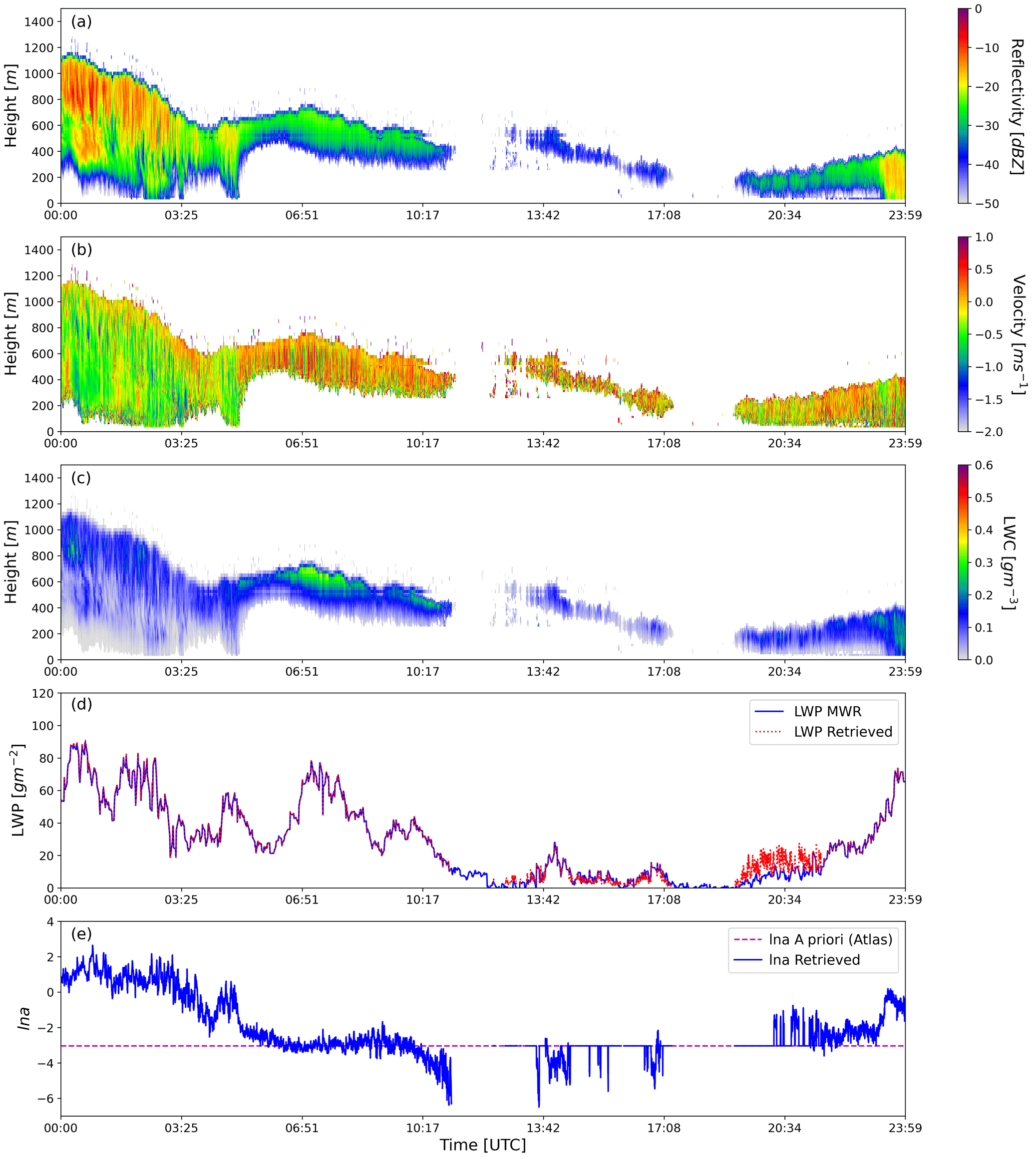
Figure 2(a) Time–height plot of radar reflectivity; (b) time–height plot of vertical velocity; (c) time–height plot of retrieved LWC; (d) LWP estimated by the radiometer alone through quadratic regression, interpolated at radar time; and (e) retrieved scaling factor ln a of each profile for the 5 February 2019 case at SIRTA.
There were no overlapping clouds observed in this instance, and the airborne plankton were removed manually. A dense cloud from midnight with a cloud base close to the ground dissipates before noon, and the formation stage of fog is initiated after sunset. Throughout the day, the liquid water path remains below 100 g m−2. Reflectivity values reach 0 dBZ for a few profiles, indicating drizzle in the beginning (between 00:00 and 03:00 UTC). As indicated by radar observations, higher reflectivity values are due to drizzle, yet LWP is nearly identical for the cloud, with reflectivity as low as −35 dBZ, and contributes the least to LWP. This also explains why it is critical to have LWP information to constrain LWC retrievals, particularly for profiles with drizzle within the cloud and when it evaporates fully before reaching the ground. Figure 2c indicates a general increase in LWC towards the cloud top, and the retrieved LWC is less than 0.3 g m−3. The scaling parameter has a wide, range from −6 to +3, which supports empirical values of a in Table 1. The value of ln a changes for each profile. Therefore, this case illustration shows that the retrieval of LWC and scaling factor can be utilized to derive a climatology of the scaling factor for different cloud types. It is worth noting that the retrieval algorithm deals with all the variations in cloud types, and the behavior of scaling factors must be studied. The next section elaborates the robustness of the retrieval algorithm for various sensitivity parameters.
The goal of this section is to verify the consistency of the retrieval behavior and to assess the sensitivity of the algorithm to inputs, errors, and hypotheses. Sensitivity analysis does not replace a proper validation of algorithm retrievals. In Sect. 5, a comparison with in situ measurement is discussed. Like every other algorithm, this retrieval algorithm also suffers from some fundamental uncertainties which must be addressed. To do so, we use a sensitivity analysis approach. It can also be referred to as “what-if” analysis, where the input parameters of the model are varied one by one. As shown in the schematic of the retrieval algorithm in Fig. 1, the retrieval is sensitive to not only input parameters but also other settings like the a priori errors, expected errors in measurement, and a priori information. To quantify the sensitivity of the retrieval algorithm, real observations are not used because the true profile of LWC from an in situ sensor is not always available. Instead, synthetic data that contain all the characteristics of real observations are used to evaluate the performance of the algorithm. Maahn et al. (2020) highlighted the major benefits of using synthetic data to test algorithms and models. First and foremost, systematic forward-model errors cancel each other, and second, we know the true atmospheric state Xtruth, which can be compared with the retrieved optimal result Xret. Hence, considering the mentioned advantages, we are using synthetic data for the sensitivity analysis of the retrieval algorithm.
The flowchart of the sensitivity analysis is presented in Fig. 3, where sensitivity parameters are the parameters in the retrieval algorithm which are perturbed, and the impact is tested. The objective is to formulate input parameters from the truth, and by feeding synthetic observations to the retrieval algorithm, the result should match the truth. In the block diagram, synthetic observations (Z and LWP) are fabricated using the forward model.
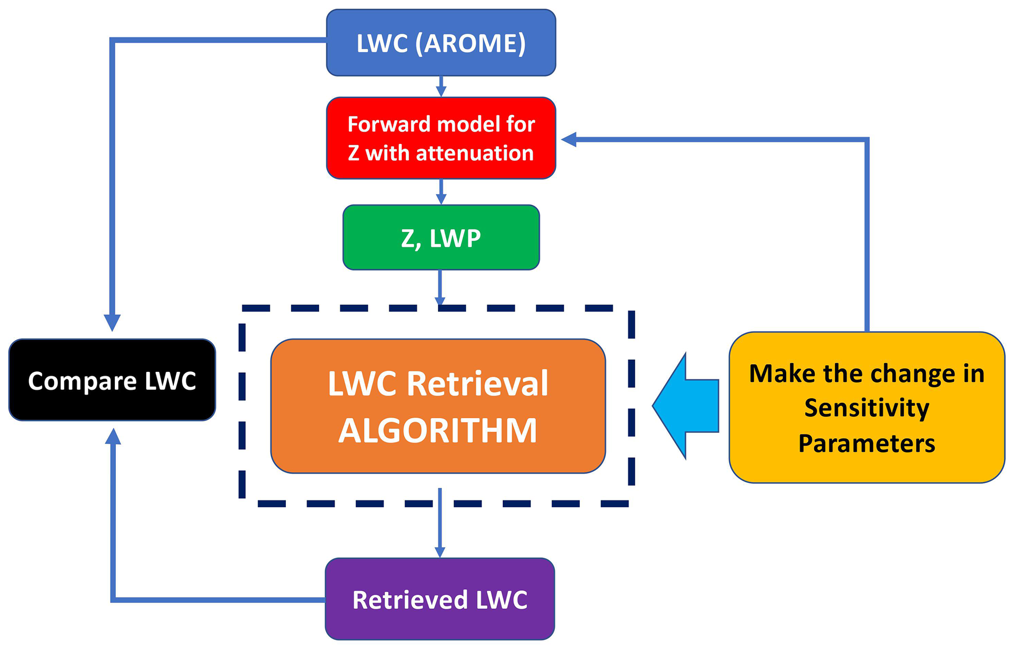
Figure 3Flow chart for sensitivity analysis of retrieval algorithm. The block inside the dashed line is the same as shown inside the dashed line in Fig. 1 with all the sensitivity parameters.
However, we are aware of the fact that the retrieval errors might be different when observed in real observation scenarios, which is already discussed in Sect. 3.2 for real observations. The error in retrieved LWC with respect to what we consider as true LWC is calculated using Eqs. (11), (12), and (13) for the entire sensitivity test.
-
Root mean square error is calculated as follows:
-
R2 (coefficient of determination) quantifies the degree of any linear correlation between observations (LWCtrue) and retrievals (LWCret). The general definition of the R2 regression score function is
where SSres is the residual sum of squares, and SStot is the total sum of squares.
-
Mean absolute percentage error measures the accuracy of the retrieval in percentage:
where LWCret and LWCtrue are retrieved and true LWC, respectively, and n is the number of data points. Analysis of each sensitivity parameter is presented in the next section.
4.1 Description of synthetic data
Synthetic data of LWC can be prepared from empirical relations, theoretical adiabatic LWC, or model forecasts. For this sensitivity analysis, we opted to include physical parameters of the 16 November 2018 fog structure simulated by the AROME model of the retrieval algorithm. The selection requirement for this instance is that it contains a sufficient number of LWC profiles to evaluate the behavior of the algorithm.
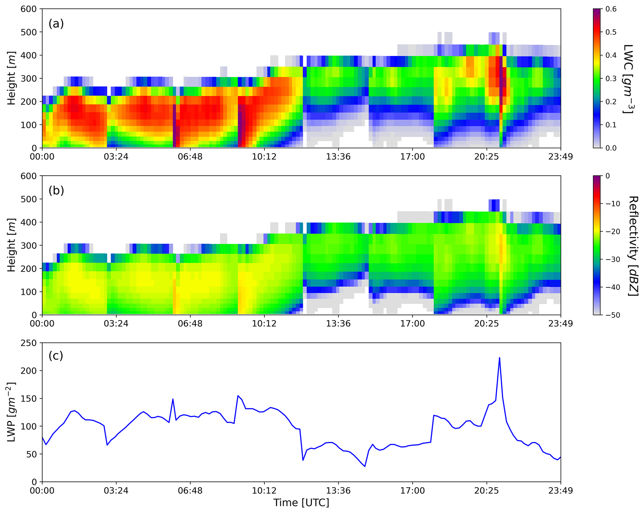
Figure 4Simulations from the AROME model for 16 November 2018 showing (a) distribution of true LWC as a function of time and height in grams per cubic meter, (b) synthetic profile of reflectivity, and (c) LWP calculated by integrating true LWC.
AROME is a French convective-scale numerical weather prediction (NWP) model, operational since 2008, covering France and western Europe and providing high-resolution simulations of fog forecasts at 1.3 km horizontal resolution and 90 vertical levels of 144 profiles. The detailed setup of the AROME model and fog forecast is explained in Bell et al. (2021). LWC of a fog structure from AROME short-term forecasts at the nearest grid location of SIRTA is considered the true atmospheric state. In this case, we are considering only liquid droplets, with no overlapping of liquid or ice clouds aloft. Profiles of true LWC are used to synthesize observation parameters like radar reflectivity using the previously defined power law relation and the liquid water path of each profile by integrating true LWC at each pixel. The forward model (block in red) consisting of the power law relation and attenuation correction model for deriving the synthetic profile of Z using coefficients a and exponent b is taken from the Atlas (1954) empirical relation. The two-way attenuation correction applied to Z is calculated from Eq. (7) (see Fig. 4).
One of the most obvious sources of uncertainty in the retrieval is the observation (calibration errors and instrumental noise) and forward-model errors. The forward-model errors tested in this sensitivity analysis are the variation in attenuation consideration and the variation in exponent b. As the observation vector, Y contains measurements from two independent instruments, bringing random and uncorrelated errors within the elements of Y (Maahn et al., 2020). The deposition of liquid droplets on the radome introduces an additional bias in radar observations. This is tested by analyzing the impact of possible biases in Z. The next sections cover the sensitivity analysis of the retrieval algorithm for perturbations in different parameters.
4.2 Sensitivity analysis of impact of error in observation
The input for synergistic retrieval in the observation vector Y consists of concatenated observations from the cloud radar and the radiometer. Each instrument has different errors, and it is worth mentioning that in the case of radar observations, instrumental errors are considered for each gate, whereas for the LWP measurement from the radiometer the observation error is estimated over the entire cloud profile, i.e., an integrated measurement. By varying the weight of instrumental error from each observation (Z and LWP) and keeping the rest constant, the impact on the retrieved LWC is compared with the true LWC.
Observation errors are assumed to be independent, and the synthetic observations of Z and LWP are calculated using true LWC, as shown in Fig. 4. Equation (7) is used to calculate attenuation due to liquid water in the synthetic profile as well as in the forward model. A priori information of LWC is calculated using synthetic reflectivity and the scaling factor from the empirical relation proposed by Fox and Illingworth (1997). Since we are looking at the impact of observation error, the retrieved parameters should have the least contribution from a priori information, and therefore high a priori error (1000 % in this case) is considered. Because the a priori estimate of LWC is derived from synthetic Z, the a priori information employed in the retrieval must differ from the true LWC to minimize the contribution of a priori information, which forces retrieval to be close to true LWC.
Table 4Different configurations of error in measurement and respective statistical errors in retrieved LWC with respect to true LWC.
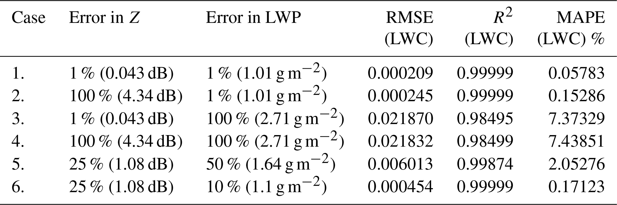
Table 4 shows the combinations of errors in measurements of Z and LWP considered in the retrieval, and the errors are calculated for retrieved LWC with reference to true LWC. Cases 3 and 4 in Table 4 indicate that the retrieval is more sensitive to errors in LWP as compared to errors in Z with approximately the same mean absolute percentage error in LWC of 7 %, whatever the assumed errors in Z. This is because for each profile there is only one LWP value which impacts the whole profile for a given error, but for error in reflectivity, only the associated pixel is impacted. With the increase in percentage errors in LWP measurement from 1 % to 100 %, the RMSE in LWC is also increased approximately 100 times, further demonstrating the high sensitivity of the algorithm to the LWP.
Delanoë and Hogan (2008) likewise incorporate a 1 dBZ uncertainty in the measurement of Z for ice cloud retrieval using 95 GHz radar with lidar and the microwave radiometer. However, error in LWP has a very low difference in MAPE and RMSE when 1 % to 10 % error is considered. Therefore case 6 in Table 4 is an optimum balance of observational error for Z and LWP. This combination of errors in measurement is used in all the retrieval cases presented in Sects. 3.4 and 5.1.
4.3 Sensitivity analysis of impact of attenuation due to liquid droplet model
In this section, the sensitivity of the attenuation model considered in the algorithm to retrieve LWC is highlighted. Wet radome can cause up to 20 dBZ of two-way attenuation due to rain in the reflectivity (Delanoë et al., 2016), but attenuation due to fog is far less than 20 dBZ. Two attenuation relations for liquid clouds from the literature are used to test the sensitivity of the algorithm. Equation (7) is proposed by Vali and Haimov (2001), in which attenuation is a function of LWC (abbreviated as Att (LWC) in Table 5), and the relationship in Eq. (8) is proposed by Vivekanandan et al. (2020), where attenuation is the function of radar reflectivity factor (abbreviated as Att (Z) in Table 5). Both of these relationships are derived using in situ observations from 95 GHz radar mounted on a research aircraft. The forward model with different attenuation relationships in the algorithm is tested for synthetic Z and LWC. To fabricate synthetic Z, the power law relation with a=0.012 and b=2 (in Eq. 1) is used. Different combinations of attenuation correction in the synthetic profile and in the retrieval algorithm are tested, as shown in Table 5. A priori information for state parameters is calculated from the Atlas (1954) empirical relation with an a priori error of 1000 %, and the measurement errors for Z and LWP are considered to be 25 % and 10 %, as discussed in Sect. 4.2. The comparison of bias in LWC for the attenuation model is shown in Fig. A1 (see Appendix).
Table 5Variation in a priori error and different errors calculated with respect to true LWC.
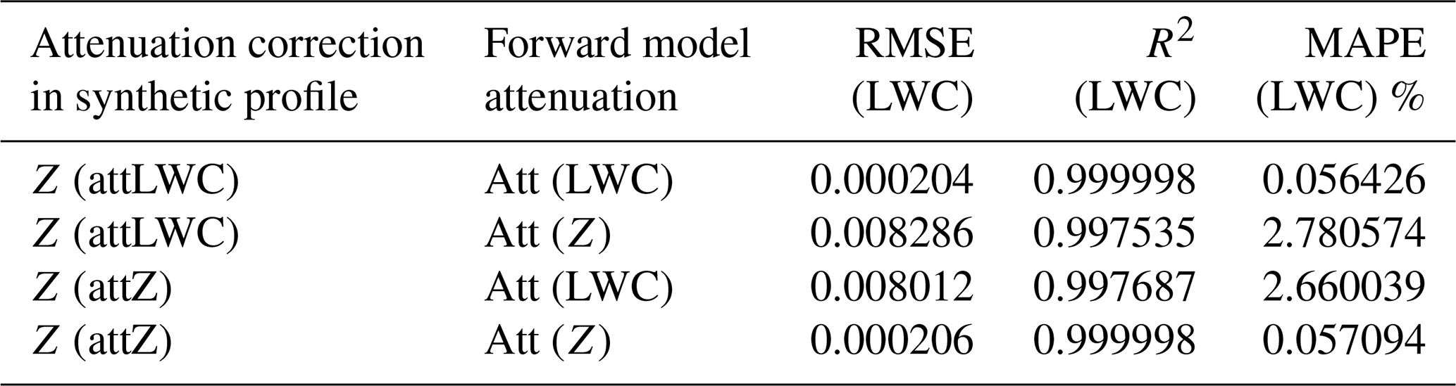
Retrieved LWC considers the same attenuation correction in the synthetic Z profile and in the forward model; RMSE is 0.0002, and MAPE is as low as 0.05 % as all the parameters are identical. But when the attenuation relation is exchanged for the synthetic profile and the forward model, MAPE increase to 2.7 %. The distribution of bias in LWC over the profile is different because attenuation due to LWC estimated by two relations is different, and thus the estimated LWC is also different. A similar test for attenuation with different “a” in the power law relation gives the same errors when the retrieved LWC is compared with true LWC. Bias in LWC for considering the same attenuation relation in the synthetic profile and the forward model is found to be close to zero. Therefore, the sensitivity test for attenuation indicates that attenuation correction of Z has very low impact, and it can bring up to 2.7 % mean absolute percentage error in retrieved LWC when the wrong attenuation model is used.
4.4 Sensitivity analysis of bias in Z and LWP
Bias in observation is the systematic error added in measurement, which can be due to the error in calibration of any instrument or transfer function of the measurement. Therefore, it is necessary to test the behavior of the retrieval algorithm for such systematic biases in measurement. For the test cases of biases, the error in the observation vector is considered to be 25 % and 10 % for Z and LWP, with a priori information of LWC calculated using a=0.012, as proposed in Fox and Illingworth (1997), and a=0.012 is used as ln a a priori. This test is to analyze the impact of bias in measurement on retrieval. Therefore, the a priori information should have a minimum contribution, and hence 1000 % error in the a priori estimate of LWC and ln a is considered. In this analysis, only one of the two observations is biased at a time to see the individual impact on retrieval. It is assumed that the bias in Z is 2 dBZ considering that error in calibration in BASTA radar measurements is around 1 to 2 dBZ (Toledo et al., 2020). The bias in LWP estimation is considered to be 10 g m−2, which is supported by Wærsted et al. (2017) for this sensitivity test.
The order of error in retrieved LWC with respect to true LWC is much higher for 10 g m−2 bias in LWP than 2 dBZ bias in Z. However, bias in the two measurements is not comparable because the parameter Z is measured over each pixel, and LWP is a single point measurement for the whole column. Since the bias applied to Z applies to each cloud pixel, and the bias applied in LWP is integrated for the whole profile, 11 % MAPE in LWC is observed, which again indicates the sensitivity of retrieval for LWP. Another reason for the difference in LWC is due to the fact that Z is in the log scale, and error in observation allows more spread in Z (25 %) than in LWP (10 %); therefore, the impact on LWP is larger. The bias in Z is propagated in ln a, but the bias in LWP directly impacts LWC. The simultaneous biases in Z and LWP have also been tested, which reveals that the bias in LWP dominates over the bias in Z, with 11 % MAPE when these biases are considered in Z and LWP.
4.5 Sensitivity analysis of LWP assimilation
The impact of adding LWP information in the retrieval is evaluated by comparing LWC retrievals in the situation where LWP information is assimilated with those in the case where it is not assimilated. For the case when LWP is not assimilated, the pre-factor a is not retrieved and hence kept constant. Different scaling factor ln a values are selected from various empirical relations listed in Table 1, and the error in retrieved LWC is calculated with respect to true LWC for each fixed scaling factor ln a value.
In this subsection, the synthetic profile of Z is fabricated using the power law with constant a and b proposed by Atlas (1954) and LWC provided by the AROME model. Table 7 contains the scaling factors taken from the empirical relations used to retrieve LWC without LWP assimilation. The MAPE is calculated for retrieved LWC for each ln a value. In Table 7 the highest value of MAPE is observed when a=0.012, and the lowest value is for a=0.048, which is the exact value of ln a used to fabricate Z. As the value of the scaling factor ln a differs from the scaling factor used to fabricate the synthetic profile (here ln a is from the Atlas, 1954 relation), the error in retrieved LWC with respect to true LWC also increases.
On the other hand, when the LWP information is assimilated in the retrieval, the MAPE in retrieved LWC compared to true LWC is decreased down to 0.171 %. However, it is not likely that the LWP is always accurate, as LWP is not a direct measurement but obtained from a retrieval algorithm and can have both random and systematic errors. Therefore, one must test the retrieval algorithm when the LWP information is biased. The retrieval technique is now evaluated for different biases in LWP information. As already mentioned, when we assimilate LWP information, the scaling factor is allowed to vary. We tested the retrieval with varying biases, as shown in Table 8, where case 2 has the same error as cases 1 and 2 of Table 6. The highest value of LWP in the synthetic profile is approximately 240 g m−2. We added the biases in LWP from ±5 to ±50 g m−2, which shows 5.5 % to 56 % MAPE in LWC.
Fox and Illingworth (1997)Sauvageot and Omar (1987)Krasnov and Russchenberg (2005)Atlas (1954)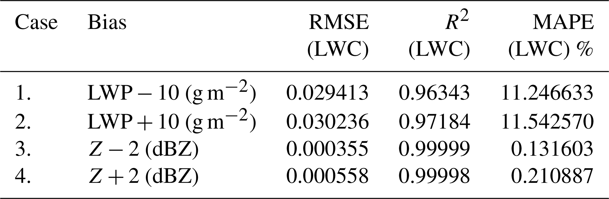
Table 7Error in retrieved LWC for fixed a when LWP is not assimilated.
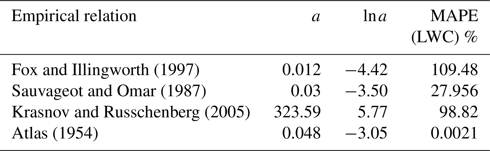
Table 8Error in retrieved LWC for various biases in assimilated LWP.
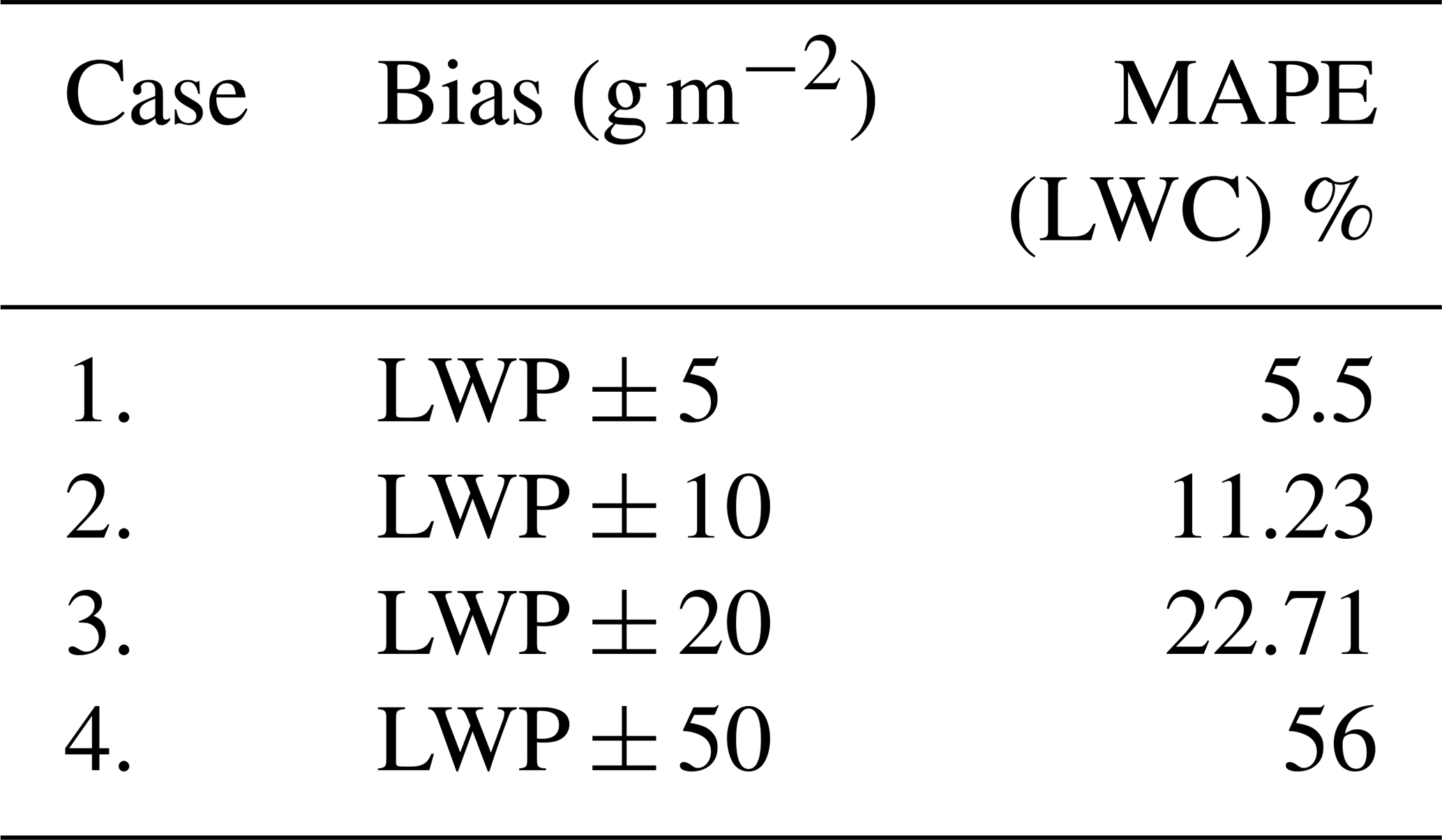
These errors are summarized in Fig. 5, where the olive green bars indicate the MAPE in LWC for different values of ln a obtained from the retrieval without LWP assimilation. The blue color bars are the MAPE in LWC for various biases when the MWR LWP is assimilated. It is clear from this comparison that the assimilated LWP, even if the product is biased, has a lower error than the retrieval case that does not assimilate LWP.

Figure 5Errors in retrieved LWC when LWP is not assimilated (green bars), as compared to those when LWP is assimilated and affected by different values of biases (blue bars). The y axis represents the MAPE in LWC, and the x axis shows the value of ln a taken from empirical relations and assumed biases in LWP.
4.6 Sensitivity of parameter b
The exponent b from the power law equation (Eq. 1) is considered to be 2 for all the cases discussed in this paper; however, the range of parameter b in the literature is proposed from 1 to 2. To test the impact of variation in b on the retrieval algorithm, the value of b was used to fabricate synthetic observations Z and LWP, and b values in the forward model are the same. Keeping all the other settings constant, the error in retrieved LWC should be due to changing b. Table 9 shows the range of b and the respective error in retrieved LWC with respect to true LWC. The retrieved LWP matches with the assimilated LWP; only the distribution of LWC is changed, observed to be the lowest for b=2. Figure A2 (see Appendix) shows that the cost function is also the lowest for b=2, and MAPE in LWC is twice that when the value of b is taken as 1.

There is a negligible impact of variation in b over ln a as shown in Fig. A2, and the error in LWC is between 0.35 % and 0.17 %. The convergence is achieved with a lower cost function, and MAPE in LWC is also the lowest for the b=2 case. Because ln a is allowed to be variable in the forward model, it is most likely that the change in b is compensated by the change in ln a.
4.7 Analysis of the sensitivity exercise
In conclusion, since this sensitivity test was performed on a synthetic profile, the overall impact of uncertainty in each parameter on the retrieval can be very different when applied to a real profile. However, an estimate of errors can be made using this exercise. The error in observation must be chosen very carefully for retrievals. A 25 % error in Z is also supported by realistic calibration error in BASTA radar, which was calculated between 1 and 2 dBZ using a 20 m mast (Toledo et al., 2020), where 25 % error in Z corresponds to 1.08 dBZ. This combination of 25 % and 10 % error in measurement has only 0.17 % MAPE when tested with a synthetic profile, which is why this combination is used in the algorithm. The a priori information must be considered only to stabilize the retrievals for unavailable measurements, otherwise the a priori error can be kept high. The a priori estimate is a constraint for the entire retrieval; hence the uncertainty in the retrieval must be smaller than the a priori error. Otherwise, the retrieval does not add any information from the observations (Maahn et al., 2020). Retrieval is very sensitive to the bias in LWP as LWP is point information for the whole cloud column; therefore error in observation and biases in Z and LWP both play a very critical role in the retrieval. Furthermore, the sensitivity analysis also revealed that incorporating LWP even if it is affected by a bias is better than not assimilating LWP information. The sensitivity of retrievals for parameter b shows the least error when b=2 because this is the same used to fabricate Z synthetically from the true LWC. Nevertheless, it is worth noting even with other values of b that the MAPE does not exceed 0.35 %.
In situ measurements of cloud and fog are required to validate the distribution of LWC with time and height. In general, in situ measurements of cloud microphysical parameters are collected using a research aircraft mounted with sensors flying inside the cloud. During the SOFOG-3D field experiment, a tethered balloon equipped with in situ sensors was used to collect the microphysical parameters of fog. This approach is much more economical than the research aircraft flying inside the cloud; however, the trajectory of the balloon cannot be fully controlled, and the measurements are limited to the lowermost 1–2 km level. Simultaneous measurements using remote sensing instruments like BASTA cloud radar, a microwave radiometer, and automatic weather stations were also collected for various fog cases (Martinet et al., 2020). Since the LWC retrieval algorithm described in previous sections essentially works with liquid clouds including fog, measurements collected during the SOFOG-3D experiment are well suited to validate the algorithm. The input for the algorithm is taken from vertically pointing cloud radar reflectivity and LWP estimates from MWR measurements. Retrieved LWCs are then compared with the measured LWC using in situ sensors.
5.1 Presentation of the case study of 9 February 2020
One fog case study observed at the super-site (44.4∘ N, −0.6∘ E) on 9 February 2020 is presented to compare retrieved LWC with in situ measurements collected from the tethered balloon. This case is selected because fog and stratus clouds were observed, allowing us to establish a comparison of retrievals with in situ observations for two different cloud types at once. The observations from vertically pointing radar and MWR are used to retrieve LWC with exactly the same algorithm described in previous sections. During this experiment, MWR was set up to collect boundary layer scan at lower elevation angle down to 4∘ every 10 min, and therefore the LWP is interpolated for such gaps. Relying on the previously led sensitivity study, error in observations for Z and LWP is taken as 25 % and 10 %, respectively, with the a priori information calculated from the Atlas (1954) empirical relation. The a priori error is considered to be 1000 %, which is the same as that mentioned in Sect. 3.2 when MWR information is available. As stated in Sect. 3.2, radar misses a few low-level gates near the ground due to antenna coupling, which contains critical fog information. The properties of fog are assumed to remain constant between the first available gates and the ground, and thus reflectivity is extrapolated (extended) downwards for the unavailable range gates. The fog shown in Fig. 6 sustained for 4 h and then started dissipating to form a stratus cloud. The visibility observed at the super-site is also less than 1000 m until 04:00 UTC. The discontinuity in radar reflectivity close to 200 m is due to the beam overlap correction used in the L2 product of BASTA.
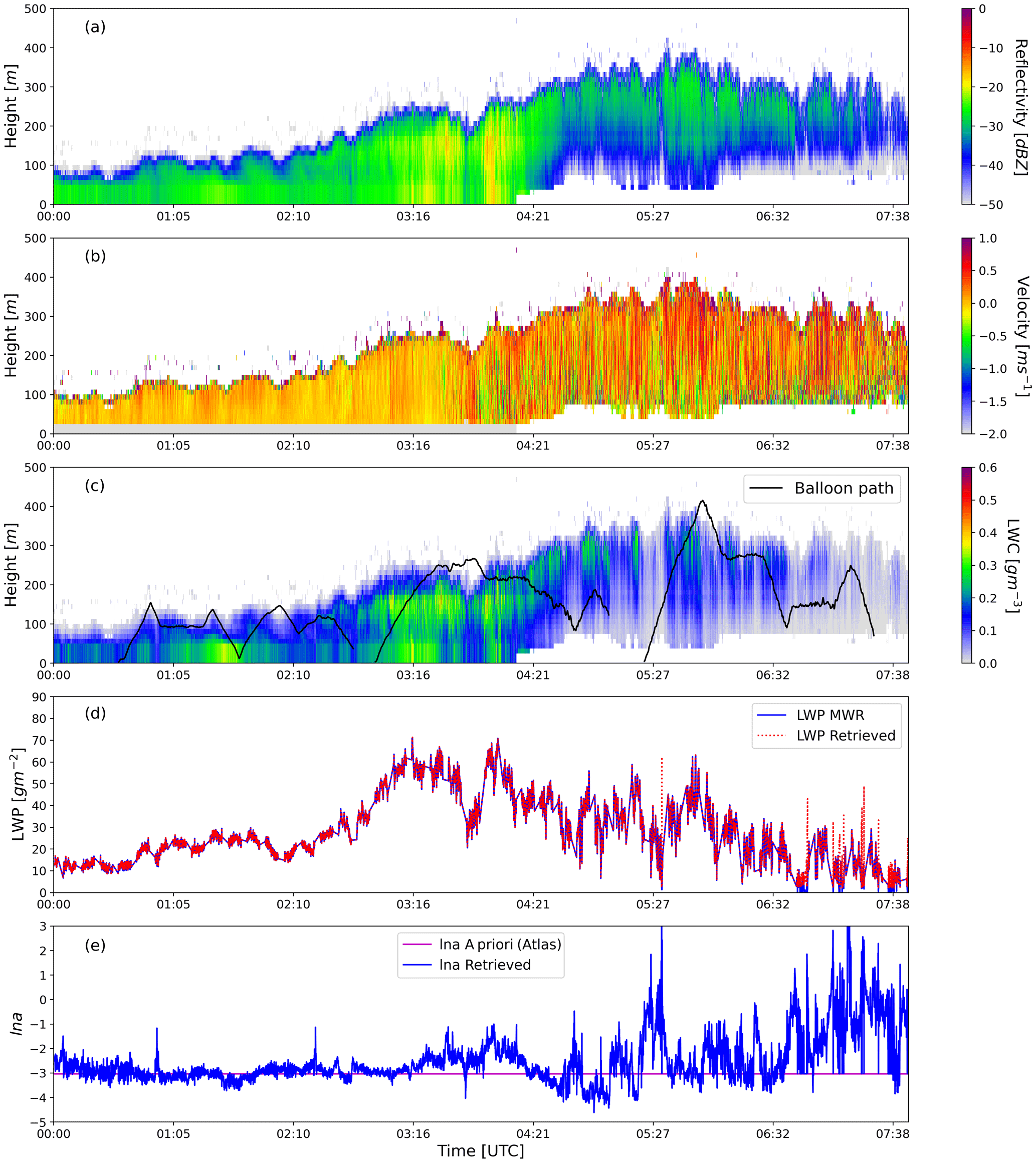
Figure 6(a) Radar reflectivity Z extended to the lowest gates, (b) Doppler velocity plotted only for the available gates, (c) retrieved LWC, (d) LWP, and (e) retrieved ln a for the 9 February 2020 case at the SOFOG-3D super-site. The tethered balloon trajectory over retrieved LWC is shown by the black line.
5.2 Comparison between in situ and radar measurements
To compare the retrieved LWC with in situ measurement, the co-location of tethered balloon data with BASTA reflectivity points is accomplished by determining the closest radar gate that corresponds to the balloon height.
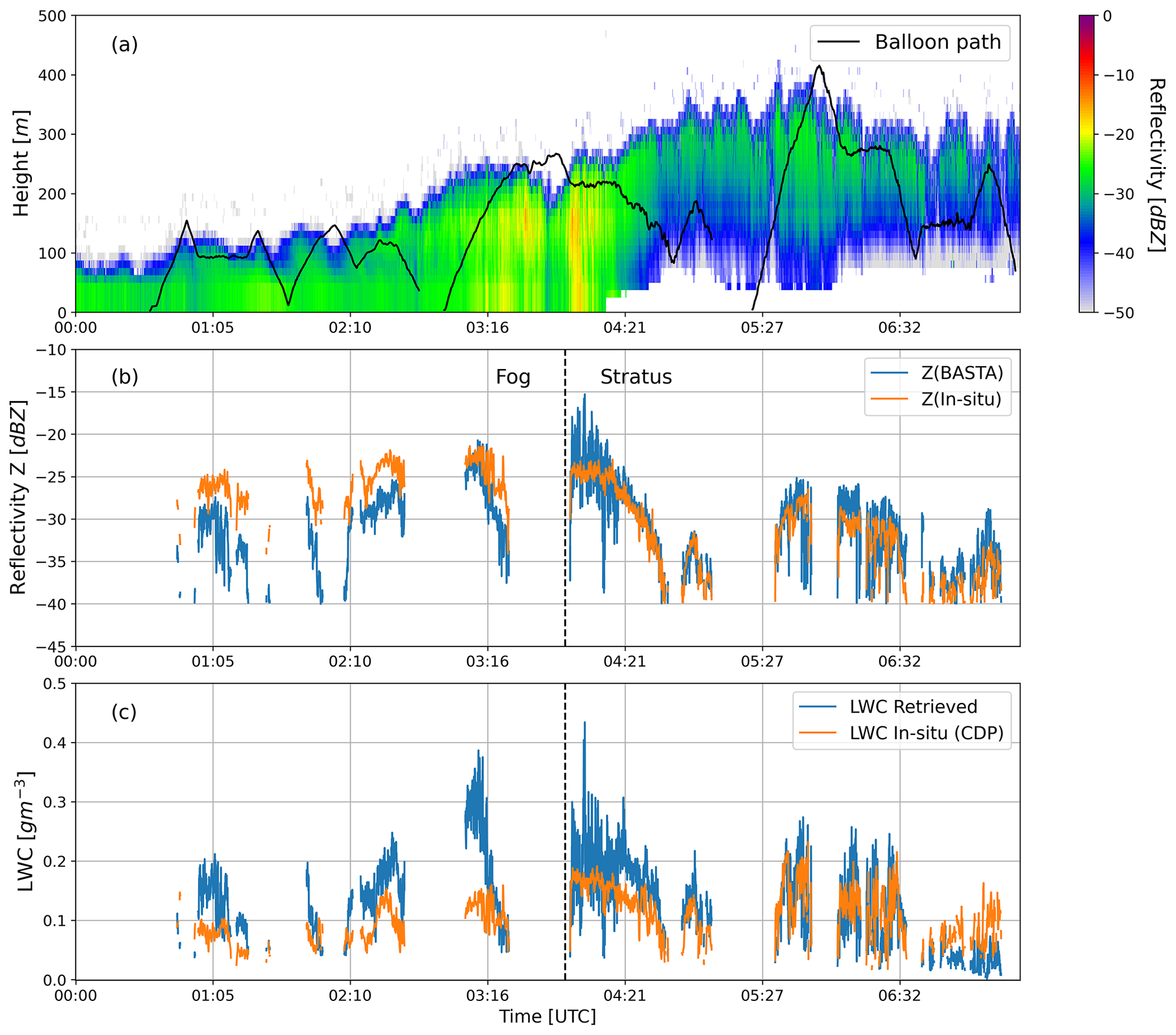
Figure 7(a) Radar reflectivity and balloon path, (b) comparison of radar reflectivity with reflectivity calculated from CDP using DSD, (c) comparison of retrieved LWC with in situ LWC.
In Fig. 7b and c, the dashed black line indicates that the visibility is more than 1000 m from 04:00 UTC onwards and therefore separates fog and stratus clouds. Since the balloon also contaminates the radar measurement, all the co-located points when the tethered balloon was within the radar detection range are eliminated. The maximum distance observed between the tethered balloon and BASTA radar was 700 m. The radar reflectivity factor from in situ measurements is calculated using the 6th moment of the droplet distribution measured by CDP. Note that the radar reflectivity is still in the Rayleigh regime as the measurements from CDP cannot exceed 50 µm. The co-located points with reflectivity less than −40 dBZ are masked because the signal-to-noise ratio for radar is low.
In Fig. 7b the radar reflectivity from BASTA and CDP are compared for the co-located points and indicates a clear bias for fog and relatively much better agreement for stratus clouds with −4.44 dBZ mean bias for fog and 0.89 dBZ for stratus clouds. The bias is calculated as the difference between ZBASTA and Zin situ. The root mean square error (RMSE) in Z is 5.2 dBZ for fog and 2.8 dBZ for stratus clouds. Figure 7c shows the comparison of the retrieved LWC values with LWC observed by CDP at the co-located points of the balloon trajectory. The mean bias in LWC for fog is 0.06 g m−3, and for stratus clouds it is 0.009 g m−3. The RMSE in LWC for fog is 0.082 and 0.056 g m−3 for stratus clouds. The comparison of retrieved LWC with in situ observations of LWC from CDP resulted in a root mean square error of 0.067 g m−3 including fog and stratus clouds.
If a well-calibrated radar samples the same cloud column and has a similar sensitivity to DSDs, the in situ reflectivity estimate should match the radar reflectivity. However, the sensitivity of the CDP sensor is limited to sampling the droplet diameters from 2 to 50 µm, while radar can sample a wider range of DSDs and is more sensitive to the largest droplets. The variations in comparison with in situ observations are noticed when the balloon is close to the cloud edge, where a slight difference in altitude can significantly impact Z and LWC due to the heterogeneity of this area.
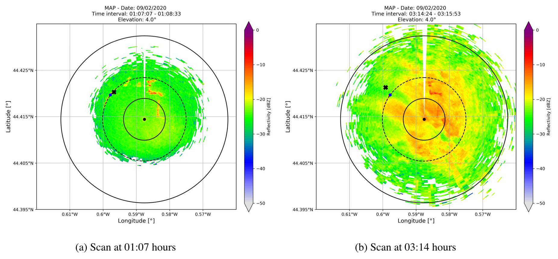
Figure 8Scans of BASTA-mini collected for fog at 4∘ elevation angle. The vertically pointing radar shown as a blue dot was located 1 km away from the scanning radar, and the cross represents the location of the balloon.
The observed differences in simulated Z and radar measurements could be explained by the vertical and horizontal heterogeneity of the fog, which strongly depends on the fog maturity. To further investigate the fog stages, a broader perspective beyond the vertical profile of fog is required. Multiple remote sensing and in situ instruments were operated simultaneously as part of the SOFOG-3D campaign to explore various fog properties. A 95 GHz scanning radar called BASTA-mini has been centered 1 km away from the vertically pointing radar, and the 360∘ scan of fog is presented in Fig. 8a and b. Plan position indicators (PPIs) of scanning radar shown in Fig. 8a and b are collected at 4∘ elevation angle. Note that this low elevation of radar can also be contaminated by the ground clutter, indicating locally high reflectivity. In Fig. 8b, a larger spread of fog is observed, which is due to the development of thicker fog.
Due to the constant evolution of fog stages and the horizontal heterogeneity of fog, the sampled volume away from the vertically pointing radar will also have distinct Z and LWC. As shown in Fig. 8b, the distribution of reflectivity on the left- and right-hand sides of scanning radar is different. Therefore, the mismatch in Z and LWC can be explained by different radar and CDP sampling volumes. As the fog lifted into the stratus cloud around 04:00 UTC, we can observe a better agreement in Fig. 7b and c, which could be explained by a more homogeneous situation. Furthermore, as shown in Fig. 7a, samples are not collected at the cloud edge for stratus clouds and therefore have lower uncertainties in Z and LWC.

Figure 9Comparison of in situ LWC and radar reflectivity relation with the (a) available literature for fog and clouds, (b) retrieved LWC and BASTA radar reflectivity relation.
To have a better idea of the representativeness of CDP in situ data, we compare LWC from BASTA and in situ measurements with LWC from simulated reflectivities obtained with DSD and empirical Z–LWC relationships (Fig. 9). Various Z–LWC relations for clouds are included in Table 1 but are not proposed for fog. In Dupont et al. (2018), linear fits for fog are proposed based on in situ observations from the tethered balloon and BASTA cloud radar at SIRTA. As a reference for fog, Flight 1, Flight 2, and Flight 3 in Fig. 9 are the fits for three fog instances computed by relating LWC observations from a light optical aerosol counter (LOAC) sensor to BASTA measurements, as described in Dupont et al. (2018). These Z–LWC fits for fog are obtained by finding the linear fit of LWC from the LOAC sensor to the radar reflectivity Z of the closest gate from vertically pointing BASTA radar. We compared the behavior of in situ fog measurement during the SOFOG-3D campaign to that of other fog relationships. As illustrated in Fig. 9, no empirical relation from the literature, including the one derived in fog, seems to be able to represent the in situ observations of this fog situation. However, the scatter for in situ measurements of stratus clouds represents a good correlation with other empirical relations as well as with the linear fits for fog from Dupont et al. (2018). The in situ measurements separated for fog and stratus clouds clearly show different characteristics and also indicate that different reflectivity values for the same LWC can be obtained as shown in Fig. 9a. This could be because of the diverse droplet spectra in stratus clouds and fog.
The impact of various DSD characteristics during the fog stages in the simulation of different-radiation fogs is discussed in Maier et al. (2012). In the Raleigh regime, Z values might become larger as fog develops due to the increase in droplet radius, while the LWC may remain constant. This introduces a non-linear relation between LWC and radar reflectivity Z. The variability within each fog stage exhibited unique properties depending on the fog event (Maier et al., 2012).
In Fig. 9b the retrieved LWC from the algorithm with respect to BASTA reflectivity (blue scatter) matches only with the in situ observations for stratus clouds and other empirical Z–LWC relations. In situ fog indicates relatively less LWC than stratus clouds at the same radar reflectivity. For the sake of comparison with Dupont et al. (2018), we also related the in situ LWC obtained during SOFOG-3D to co-located radar reflectivity from BASTA. By correlating in situ measurements of LWC with cloud radar reflectivity, it is assumed that the radar and in situ sensor observe the same cloud volume; however, the distance between the balloon and the nearest gate of cloud radar can incorporate uncertainties. In addition to this, the sensitivity of the in situ sensor (CDP) and radar (BASTA) is considered to be the same, despite the fact that the sensitivity varies with DSDs. Generally, the cloud probes undersample the true DSD of the volume due to their limited sensitivity to larger droplets. As shown in Fig. 10, the Z–LWC fits from in situ observations are in the neighborhood of other empirical relations for reflectivity less than −30 dBZ. Since the power law relations are valid only in the Rayleigh regime, the in situ observation agrees with other empirical relations for low reflectivity. Reflectivity values greater than −30 dBZ may be attributed to larger droplets, which may or may not include a higher LWC. However, a significantly better correlation of in situ fit for stratus clouds with an empirical relation by Baedi et al. (2000) (proposed for stratocumulus clouds) indicates representativeness of in situ observations for stratus clouds. The fit for in situ fog observations still indicates less LWC at the same reflectivity and does not match with any empirical relation. These observations imply that these are either collected for large droplets beyond the CDP limit or from a different sampling volume than the cloud radar samples.
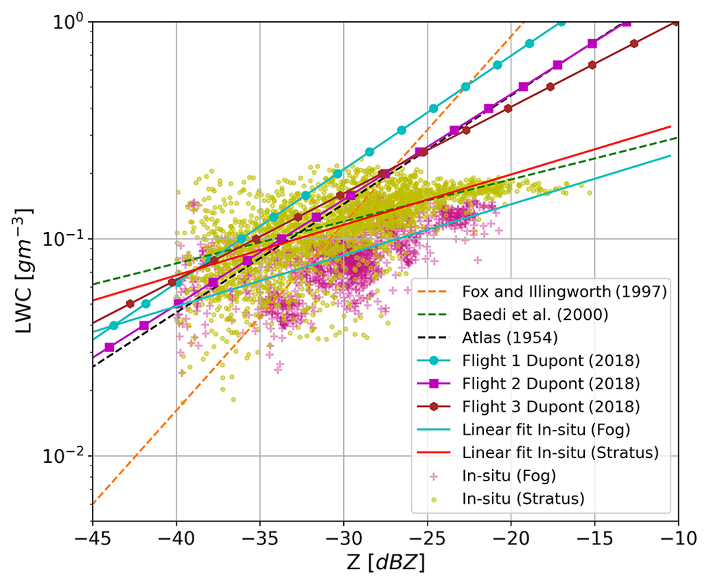
Figure 10Scatterplot for the relation between LWC measured from CDP with radar reflectivity from cloud radar, compared with the available literature. In situ measurements are separated for fog and stratus clouds where magenta denotes fog, yellow–green (chartreuse) denotes the stratus cloud, and the respective linear fits are also plotted.
Unfortunately, the limited in situ observations collected for fog and stratus clouds here do not represent a validation of the retrieval; however, this comparison highlights that there are situations more complicated than the other. Due to the non-uniform distribution of LWC in clouds or fog, homogeneity plays a key role while validating the in situ measurements. It is unfair to expect LWC to match when simulated reflectivity from in situ does not match radar measurement. In order to validate such an algorithm, in situ measurements at different heights for the same volume that radar samples are needed. However, if the in situ observation platform is positioned in proximity to the radar sampling volume, it may also contaminate the radar observations. Therefore, the in situ measurements must be collected from a homogeneous cloud to compare with the retrievals. Particularly for fog, more continuous DSD measurements, as well as the vertical profiles during distinct fog episodes, are required to produce more significant results.
The primary objective of this statistical analysis is to derive a climatology of LWC and ln a in order to allow the algorithm to be able to retrieve LWC for fog and low-level liquid clouds even when additional measurements are not available. A comparison of retrieved LWC with in situ LWC measurements for fog and stratus clouds from the SOFOG-3D experiment is already presented in Sect. 5.1. Therefore, the climatology is developed from the retrieval technique discussed in Sect. 3.4 using the larger data set from SIRTA measurements for a variety of cloud and fog incidents. Statistical analysis to derive a climatology of LWC and the scaling factor is presented in this section.
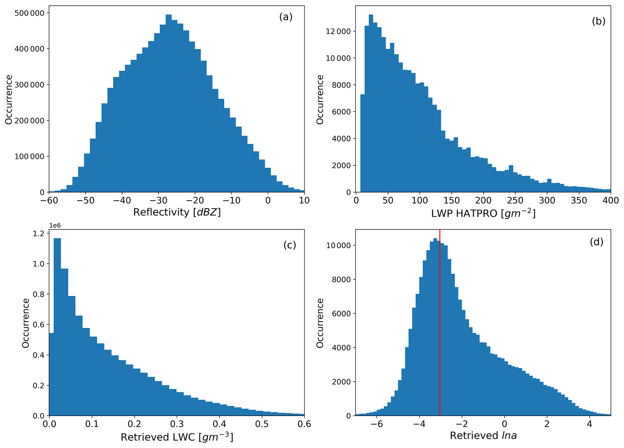
Figure 11Histogram of (a) radar reflectivity (Z), (b) LWP from MWR, (c) retrieved LWC, and (d) retrieved ln a for 39 cloudy days. The red line in the ln a histogram indicates the a priori estimate of ln a from Table 1.
The histogram of the retrieved scaling factor ln a (Fig. 11d) indicates that the highest values of occurrence are around −3, which is close to the ln a a priori value from (Atlas, 1954) the empirical relation plotted as the red line, but it is not precisely the same. The variational framework allows variability in the ln a retrieval. The assimilation of LWP brings enough information to retrieve ln a, and the spread around the a priori value is directly linked to the a priori error value. Table 1 indicates the ln a values for various cloud types proposed in the literature, which agree well with the range of retrieved ln a values. Note that there is one single ln a value for a given profile, but its value can potentially be used to differentiate clouds from the drizzle. All the profiles with rain and drizzle reaching the ground are removed for the statistics; however light drizzle with clouds and fog is discussed.
Since the algorithm does not assimilate LWP for the profiles with LWP less than 10 g m−2, the LWP histogram in Fig. 11b has no value below 10 g m−2, and maximum cloud profiles have LWP below 120 g m−2.
The parameter LWC indicates the range up to 0.6 g m−3, which includes light drizzle, while the highest number of cloud pixels have a LWC value less than 0.2 g m−3. In Fig. 12, retrieved LWC is plotted as a function of radar reflectivity for the 39 cloud cases, with Z–LWC empirical relationships from the literature for various cloud types. The black line represents the a priori estimate of the retrieval algorithm, and the higher concentration of density point overlaps with the black line is due to the profiles with LWP < 10 g m−2 where the retrieval of LWC is based on only the Atlas (1954) empirical relation. None of these profiles are considered in the climatology of ln a. However, the wide range of retrieval points indicates that the algorithm allows LWC retrieval for a variety of cloud types. The slope of the Z–LWC relationship is dependent on the value of b in Eq. (3), and because the retrieval method considers b=2, the slope of the total retrieval in Fig. 12 is constant. However, retrieval allows variability in ln a, which could partly compensate for b as well.
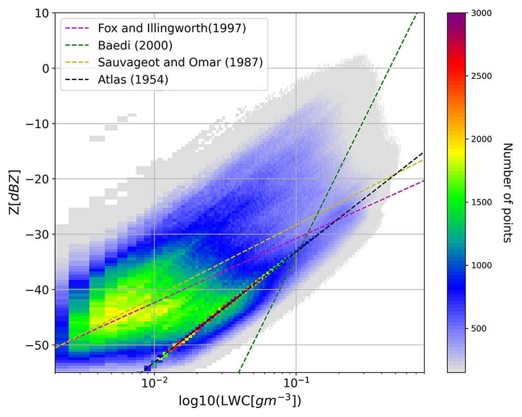
Figure 12Retrieved LWC as a function of radar reflectivity Z for 39 cloudy days, with reference plot of various empirical relations for different cloud types.
As already described, knowing LWP allows us to retrieve ln a and adjust the relationship between LWC and Z. However, when only BASTA measurements are available, we need to rely on an a priori value for ln a. Thanks to this climatology, we could both define the optimal value for this a priori and eventually propose to parametrize this value. For instance, it is envisioned to relate the scaling factor to radar reflectivity and/or Doppler velocity. As Z and V are observed for each cloud pixel, and only one value of ln a is retrieved for a given cloud profile, one single piece of reflectivity or velocity information should be associated with ln a. We propose to summarize the reflectivity and velocity information in the mean or maximum value of the profile in order to have one value per profile.
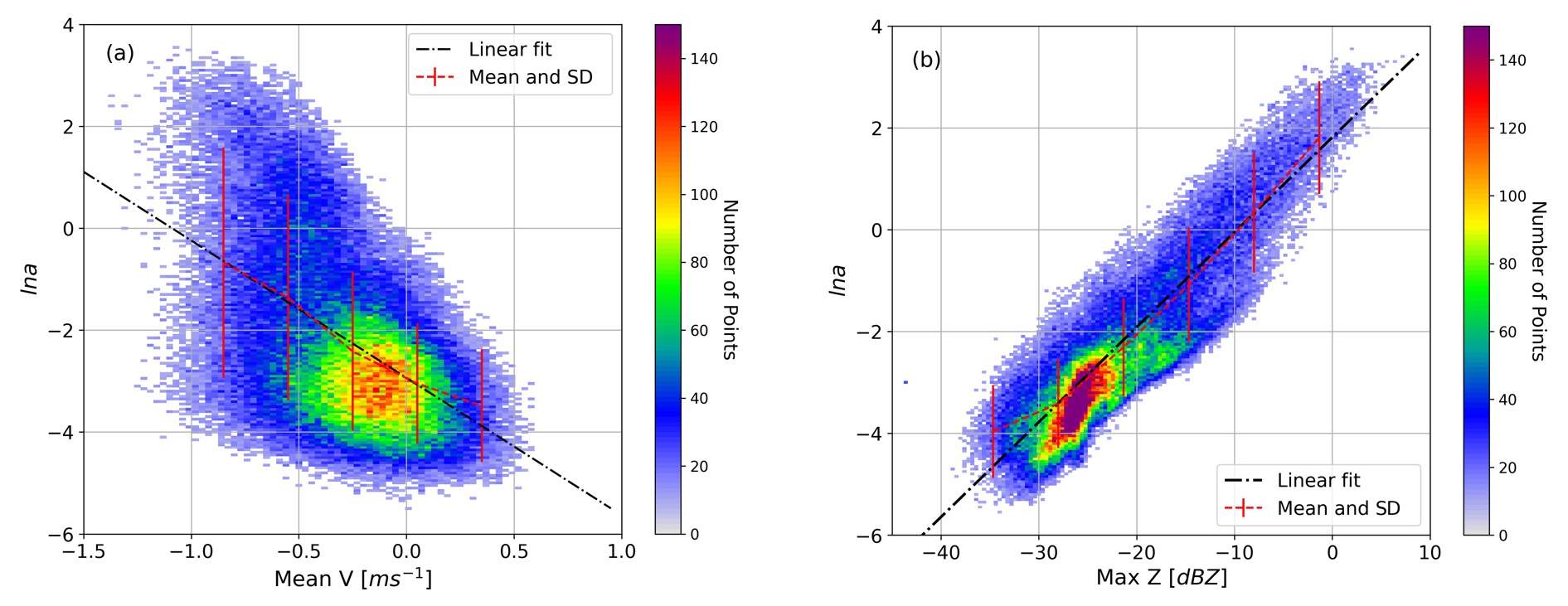
Figure 13Correlation of (a) mean velocity versus ln a and (b) maximum reflectivity versus ln a for cloud profiles, where the color bar indicates the number of profiles.
Maximum and minimum velocities of the cloud column are associated with the updrafts and downdrafts, which may not represent the complete profile for ln a. Therefore, we rely on the mean velocity of the profile. The density plot of mean velocity as a function of ln a is plotted in Fig. 13a, indicating that the mean velocity of most profiles is concentrated between −0.5 and 0.1 m s−1, which is compatible with liquid cloud sedimentation velocity. Mean velocity close to 0 m s−1 with ln a values ranging from −4 to −2 implies pure clouds, whereas few profiles with a mean velocity less than −0.5 m s−1 must be impacted by the drizzle droplets in the profile. The standard deviation plotted by the red line indicates that the variability in ln a is very high for the profiles with mean velocity below −0.5 m s−1. Due to the large standard deviation, ln a cannot be associated with mean velocity; however, velocity information can be used to classify drizzle droplets. As illustrated in Fig. 13b, a substantially stronger association is observed between maximum radar reflectivity and ln a of the profile. For most of the cloud columns, maximum reflectivity is observed between −30 and −15 dBZ. As maximum reflectivity also represents the drizzle in the cloud, the maximum reflectivity above −10 dBZ is suspected to indicate drizzle in the cloud. A high value of ln a for reflectivity above 0 dBZ also supports the empirical relation for drizzle by Sauvageot and Omar (1987), as shown in Table 1, where the ln a is given as 5.77. The standard deviation of ln a is also high for profiles with maximum reflectivity above −10 dBZ. The standard deviation of ln a is lowest, between −30 and −20 dBZ. The one-dimensional linear fit relating ln a and maximum radar reflectivity for cloud columns is shown by the dashed black line in Fig. 13b. In this figure, the maximum reflectivity of the profile shows a better correlation with ln a, and the mean ln a (dashed red line) coincides with the linear fit. Therefore, the one-dimensional linear relation between ln a and maximum reflectivity (Zmax) is given by
However, an investigation by selecting 15 fog cases out of 39 cloud cases indicated that the coefficients of linear fit are slightly different for fog profiles.
To utilize the above relationships, it is necessary to differentiate between liquid clouds aloft and fog. This can be easily done by determining the cloud base height to identify fog, and hence specific climatology is applied to the profile.
In this section, we describe the stand-alone approach and its assessment using MWR LWP retrieval as a reference. The climatological relation of ln a as a function of maximum radar reflectivity in the profile is used for the BASTA stand-alone retrieval when MWR observations are unavailable.
7.1 BASTA stand-alone LWC retrieval approach
The radar is not always accompanied by an MWR, and therefore a solution must be proposed to improve the retrieval with the a priori knowledge of ln a. Since LWP information is not assimilated, thanks to the ln a climatology for clouds and fog derived in Sect. 6, this information can be used as a priori information of ln a; ln a for the profile can be linked to the maximum value of reflectivity detected in the profile using Eqs. (14) and (15) for clouds and fog, respectively.
In this case, the observation vector “y” contains only radar reflectivity of each cloud pixel, with 25 % error in measurement, whereas the state vector still contains LWC and ln a both. Therefore, the Jacobian for a cloud profile with n cloud pixels will have elements. The variational method also allows us to control the contribution of a priori information in the retrieval by providing the a priori error. A strong a priori estimate of ln a is required to constrain LWC retrieval; therefore a low priori error in ln a is employed. In these stand-alone retrieval cases, 100 % a priori error in ln a is used because the standard deviation of ln a in Fig. 13 is approximately 1, which is equivalent to 100 % a priori error. The climatology of ln a for fog from Eq. (15) is applied to the profile with a cloud base less than 80 m. Retrieval of LWC should be constrained by the a priori information of LWC only to avoid non-physical values; therefore the error in the a priori values of LWC is taken to be 1000 %. In the BASTA stand-alone retrieval setup, a priori information of LWC is calculated using the Atlas (1954) relation exactly the same as radar–MWR synergistic retrieval.
7.2 First assessment of BASTA stand-alone LWC retrieval using LWP retrieved from MWR
With the details given above, the LWC retrieval algorithm is adapted to utilize the climatology of the scaling factor with only radar reflectivity measurements from SIRTA. The BASTA stand-alone retrieval algorithm is applied to the 39 selected cloud and fog cases from SIRTA.
Due to the absence of in situ sensors at SIRTA for recording the distribution of the liquid water content in clouds and fog, the integrated LWP from the HATPRO microwave radiometer is utilized to assess the quality of the retrieved LWC for BASTA stand-alone retrieval. The retrieved LWP is calculated by vertically integrating the retrieved LWC; ln a is not a retrieved parameter because LWP information is not assimilated, and the retrieval is constrained by a strong a priori estimate of ln a derived from the climatology. However, the variational framework allows ln a to be adjusted around its climatology depending on radar reflectivity. In this case, ln a values fall within the range of known values from the literature, as shown in Table 1.
Number density of profiles with LWP ranging from 10 to 250 g m−2 are compared with LWP from BASTA stand-alone retrieval (Fig. 14). Profiles with retrieved LWP less than 50 g m−2 show good agreement with LWP from HATPRO. For the profiles with higher LWP, an increase in bias is clearly observed in Fig. 14, and the mean bias in LWP obtained as the difference between LWP from HATPRO and that retrieved is −21 g m−2. The mean absolute percentage error in LWP with respect to LWP from HATPRO is 57.15 %. The relative error in LWP shown in Fig. 15 indicates that the majority of clouds have less than 35 % error in retrieved LWP. Because the climatology of the scaling factor constrains the retrieval, effective estimation of LWC can be made using only radar information when additional information is unavailable. By investigating the origin of biases, we discovered that the profiles with light-drizzle-droplet characteristics tend to overestimate the LWP by a large margin. The improvement in stand-alone retrieval can be made by classifying clouds with and without drizzle and using specific ln a climatology for them.
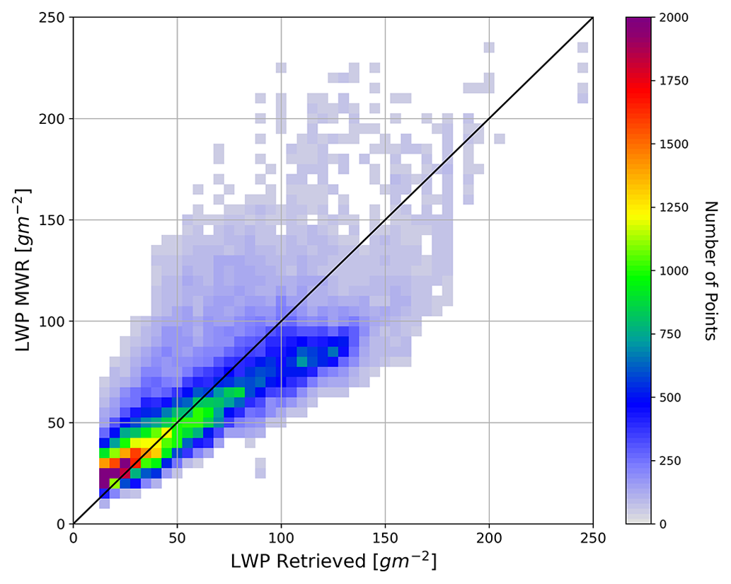
Figure 14Comparison of retrieved LWP from BASTA stand-alone retrieval algorithm with LWP retrieved by HATPRO, where the black line represents the exact match of LWP for the given profile.

An algorithm for LWC estimation of warm clouds is proposed using a vertically pointing radar and microwave radiometer synergy. The algorithm also accounts for attenuation due to liquid cloud droplets. This algorithm is based on the hypothesis that LWC is related to reflectivity with a power law fit, and one of the constants of the Z–LWC relationship is allowed to vary according to LWP retrieved by an MWR of the same cloud profile. The scaling factor ln a of the relationship is retrieved, while the exponent b is assumed constant. Therefore, the technique proposed in this study is equivalent to finding a suitable Z–LWC relationship consistent with the measured LWP for each cloud profile. This synergistic retrieval algorithm works seamlessly for liquid clouds and fog without prescribing the cloud type. The algorithm is implemented in a set of cloud and fog instances observed at SIRTA, and the analysis is discussed in this paper. These retrievals have been used to develop a climatology of LWC and the scaling factor for warm clouds and fog. The application of derived climatology to estimate LWC for stand-alone radar observations is also presented in this paper. By utilizing the climatology of the scaling factor, this stand-alone radar method can provide continuous retrieval of LWC for warm clouds even in the absence of radiometers and other additional measurements. Although this climatology is developed using measurements from the SIRTA observatory for limited cloud scenarios, a more extensive data collection from several measurement locations might be used to generate a more robust climatology of the scaling factor.
Furthermore, the retrievals are compared against in situ measurements for a fog and cloud case collected during the SOFOG-3D field campaign. The comparison of LWC values estimated using this synergistic retrieval algorithm revealed that the fog and clouds were clearly distinct. The retrieved LWC was more consistent with stratus clouds than fog. A homogeneous cloud system is required for the comparison of retrieved LWC with in situ measurements, or else the in situ sensors must sample the same cloud or fog volume as radar. To assess the accuracy of the algorithm for LWC estimates in various cloud types, in situ measurements of several types of warm clouds like fog and low-level stratus clouds with and without drizzle are required.
However, drizzle in clouds is a substantial source of error in the retrieval. Because drizzle droplets are significantly larger than cloud droplets, the power law may not be applicable in the Mie regime. As a result, the forward model exclusively for drizzle must incorporate Mie scattering or eventually another kind of relationship to link Z and LWC. A prospective work for such cloud columns is planned to separate drizzle and cloud pixels using Doppler velocity information and develop a forward model for drizzle. The variational framework discussed here can be modified to incorporate additional measurements, such as Doppler velocity. Another current limitation of our synergistic retrieval method is that it is applicable to profiles with LWP values greater than 10 g m−2. A better a priori estimate of ln a can be proposed in the future to estimate accurate LWC for low LWPs. Additionally, this retrieval method is not applicable when a mixed-phase cloud overlaps the liquid cloud layer, whereas the ice cloud above the liquid cloud does not impact the LWC retrieval of the liquid layer.
As mentioned in Sect. 3.3, the radar reflectivity profiles can be contaminated by particles in the boundary layer. In the retrieval method, these airborne plankton must be categorized and hence not processed as hydrometeors. Ultimately, a sophisticated algorithm for the classification of hydrometeors to distinguish between fog, liquid clouds, and drizzle is required. The retrieval algorithm could be updated with an improved target classification scheme to apply two different scaling factors in one profile, especially when drizzle and clouds co-occur. Also, for multi-layered liquid clouds, different ln a might be prescribed for each cloud layer with proper classification of hydrometeors. Improved classification of hydrometers for the BASTA stand-alone retrieval will improve the LWC retrieval because the range of the scaling factor varies for different categories. Further, the climatology of the scaling factor for different cloud types will improve the LWC retrieval.
We know that cloud LWC values can fluctuate both horizontally and vertically. Most liquid clouds, by their very nature, are unlikely to be homogeneous in the sense suggested as suitable here. Maybe a more statistical approach is necessary for some aspects of the retrieval comparisons. The retrieval algorithm can be validated with in situ measurements from aircraft, balloons, and UAV flights equipped with in-cloud sensors for diverse liquid clouds since UAVs and balloons travel at a slower speed than airplanes, which would allow them to sample the clouds more thoroughly. Note that some sites cannot be overflown by aircraft for safety reasons. UAVs can be more efficient in terms of controlling them remotely, as the path of tethered balloons cannot be controlled. These platforms can, however, interfere with the radar signal. In order to avoid contaminating the radar signal, the samples must be taken from a volume that is close enough and obstructs the radar the least. Before comparing the estimated values with in situ data, it is necessary to verify if the cloud volume represented by radar and in situ samples is the same. A well-mixed or homogeneous cloud system is ideal for validating such algorithms.
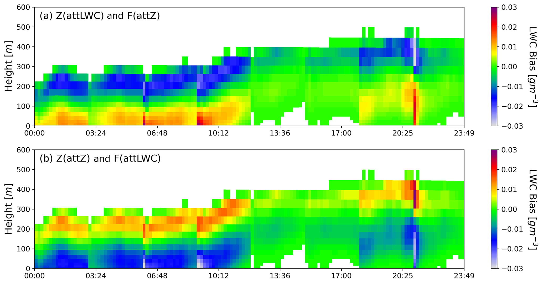
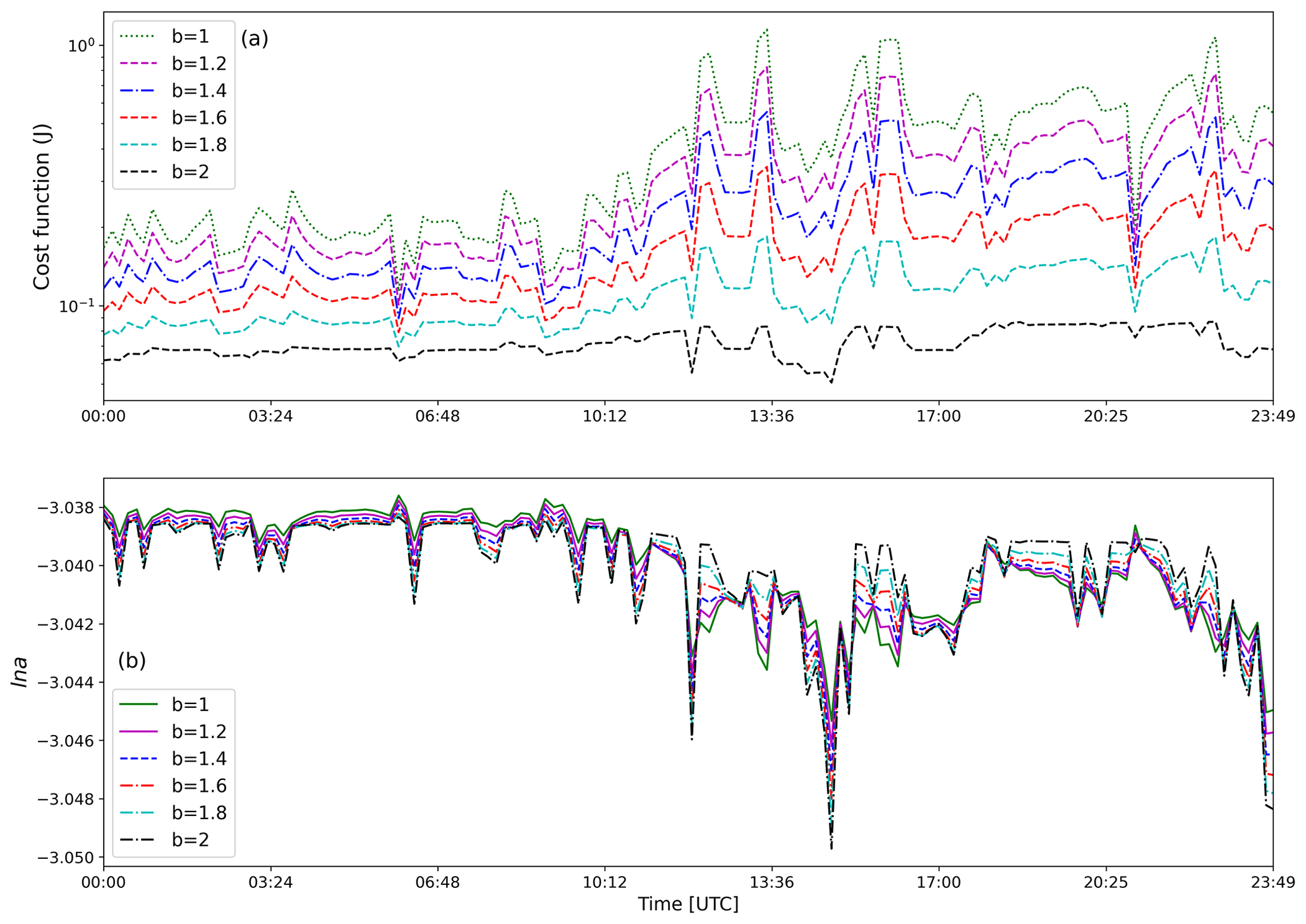
Data used from SIRTA and SOFOG-3D are publicly available from http://sirta.ipsl.fr/ (last access: 22 February 2023, SIRTA, 2023) and https://sofog3d.aeris-data.fr/ (last access: 22 February 2023, SoFog3D, 2023), respectively. Requests for cloud radar data can also be sent to julien.delanoe@latmos.ipsl.fr. The code developed in this study can be made available upon request to the authors.
PV developed the retrieval algorithm and analyzed the results with support from JD. SJ organized and preprocessed the data used in this paper from SOFOG-3D. PM provided information and data from MWR, and FB provided the CDP data from SOFOG-3D and relevant assistance. AB provided data from the AROME model used for sensitivity analysis. JCD provided the data from SIRTA. PV wrote the paper with contributions from all co-authors.
The contact author has declared that none of the authors has any competing interests.
Publisher’s note: Copernicus Publications remains neutral with regard to jurisdictional claims in published maps and institutional affiliations.
This research has been supported by the Université de Versailles Saint-Quentin-en-Yvelines (UVSQ) and Université Paris-Saclay. The authors would like to acknowledge SIRTA for providing the BASTA radar and MWR data used in this study. The authors would like to acknowledge the assistance team of the SOFOG-3D campaign for the execution of the field experiments.
This research has been supported by the French Association Nationale de la Recherche et de la Technologie (ANRT) and the company Meteomodem (Convention CIFRE).
This paper was edited by S. Joseph Munchak and reviewed by four anonymous referees.
Atlas, D.: The Estimation Of Cloud Parameters By Radar, J. Atmos. Sci., 11, 309–317, https://doi.org/10.1175/1520-0469(1954)011<0309:TEOCPB>2.0.CO;2, 1954. a, b, c, d, e, f, g, h, i, j, k, l
Baedi, R. J. P., de Wit, J. J. M., Russchenberg, H. W. J., Erkelens, J. S., and Poiares Baptista, J. P. V.: Estimating effective radius and liquid water content from radar and lidar based on the CLARE98 data-set, Physics and Chemistry of the Earth, Part B: Hydrology, Oceans and Atmosphere, 25, 1057–1062, https://doi.org/10.1016/S1464-1909(00)00152-0, 2000. a, b
Bell, A., Martinet, P., Caumont, O., Vié, B., Delanoë, J., Dupont, J.-C., and Borderies, M.: W-band radar observations for fog forecast improvement: an analysis of model and forward operator errors, Atmos. Meas. Tech., 14, 4929–4946, https://doi.org/10.5194/amt-14-4929-2021, 2021. a
Bony, S. and Dufresne, J.-L.: Marine boundary layer clouds at the heart of tropical cloud feedback uncertainties in climate models, Geophys. Res. Lett., 32, L20806, https://doi.org/10.1029/2005GL023851, 2005. a, b
Brousseau, P., Seity, Y., Ricard, D., and Léger, J.: Improvement of the forecast of convective activity from the AROME-France system, Q. J. Roy. Meteor. Soc., 142, 2231–2243, https://doi.org/10.1002/qj.2822, 2016. a
Cimini, D., Hewison, T. J., Martin, L., Güldner, J., Gaffard, C., and Marzano, F. S.: Temperature and humidity profile retrievals from ground-based microwave radiometers during TUC, Meteorol. Z., 15, 45–56, 2006. a
Crewell, S. and Löhnert, U.: Accuracy of cloud liquid water path from ground-based microwave radiometry 2. Sensor accuracy and synergy, Radio Sci., 38, 7–1, 2003. a
Delanoë, J. and Hogan, R. J.: A variational scheme for retrieving ice cloud properties from combined radar, lidar, and infrared radiometer, J. Geophys. Res.-Atmos., 113, D07204, https://doi.org/10.1029/2007JD009000, 2008. a, b
Delanoë, J., Protat, A., Vinson, J.-P., Brett, W., Caudoux, C., Bertrand, F., Chatelet, J. P. d., Hallali, R., Barthes, L., Haeffelin, M., and Dupont, J.-C.: BASTA: A 95-GHz FMCW Doppler Radar for Cloud and Fog Studies, J. Atmos. Ocean. Tech., 33, 1023–1038, https://doi.org/10.1175/JTECH-D-15-0104.1, 2016. a, b
Dupont, J.-C., Haeffelin, M., Wærsted, E., Delanoe, J., Renard, J.-B., Preissler, J., and O’Dowd, C.: Evaluation of Fog and Low Stratus Cloud Microphysical Properties Derived from In Situ Sensor, Cloud Radar and SYRSOC Algorithm, Atmosphere, 9, 169, https://doi.org/10.3390/atmos9050169, 2018. a, b, c, d
Ellis, S. M. and Vivekanandan, J.: Liquid water content estimates using simultaneous S and Ka band radar measurements: DUAL-WAVELENGTH RADAR LWC ESTIMATES, Radio Sci., 46, RS2021, https://doi.org/10.1029/2010RS004361, 2011. a
Fan, J., Wang, Y., Rosenfeld, D., and Liu, X.: Review of Aerosol–Cloud Interactions: Mechanisms, Significance, and Challenges, J. Atmos. Sci., 73, 4221–4252, https://doi.org/10.1175/JAS-D-16-0037.1, 2016. a
Fox, N. I. and Illingworth, A. J.: The Retrieval of Stratocumulus Cloud Properties by Ground-Based Cloud Radar, J. Appl. Meteorol. Clim., 36, 485–492, https://doi.org/10.1175/1520-0450(1997)036<0485:TROSCP>2.0.CO;2, 1997. a, b, c, d, e, f
Frisch, A. S., Fairall, C. W., and Snider, J. B.: Measurement of Stratus Cloud and Drizzle Parameters in ASTEX with a Kα-Band Doppler Radar and a Microwave Radiometer, J. Atmos. Sci., 52, 2788–2799, https://doi.org/10.1175/1520-0469(1995)052<2788:MOSCAD>2.0.CO;2, 1995. a
Frisch, A. S., Feingold, G., Fairall, C. W., Uttal, T., and Snider, J. B.: On cloud radar and microwave radiometer measurements of stratus cloud liquid water profiles, J. Geophys. Res.-Atmos., 103, 23195–23197, https://doi.org/10.1029/98JD01827, 1998. a
Geerts, B. and Miao, Q.: The Use of Millimeter Doppler Radar Echoes to Estimate Vertical Air Velocities in the Fair-Weather Convective Boundary Layer, J. Atmos. Ocean. Tech., 22, 225–246, https://doi.org/10.1175/JTECH1699.1, 2005. a
Haeffelin, M., Barthès, L., Bock, O., Boitel, C., Bony, S., Bouniol, D., Chepfer, H., Chiriaco, M., Cuesta, J., Delanoë, J., Drobinski, P., Dufresne, J.-L., Flamant, C., Grall, M., Hodzic, A., Hourdin, F., Lapouge, F., Lemaître, Y., Mathieu, A., Morille, Y., Naud, C., Noël, V., O'Hirok, W., Pelon, J., Pietras, C., Protat, A., Romand, B., Scialom, G., and Vautard, R.: SIRTA, a ground-based atmospheric observatory for cloud and aerosol research, Ann. Geophys., 23, 253–275, https://doi.org/10.5194/angeo-23-253-2005, 2005. a, b
Hartmann, D. L., Ockert-Bell, M. E., and Michelsen, M. L.: The Effect of Cloud Type on Earth's Energy Balance: Global Analysis, J. Climate, 5, 1281–1304, https://doi.org/10.1175/1520-0442(1992)005<1281:TEOCTO>2.0.CO;2, 1992. a
Hogan, R. J.: A Variational Scheme for Retrieving Rainfall Rate and Hail Reflectivity Fraction from Polarization Radar, J. Appl. Meteorol. Clim., 46, 1544–1564, https://doi.org/10.1175/JAM2550.1, 2007. a
Hogan, R. J., Gaussiat, N., and Illingworth, A. J.: Stratocumulus Liquid Water Content from Dual-Wavelength Radar, J. Atmos. Ocean. Tech., 22, 1207–1218, https://doi.org/10.1175/JTECH1768.1, 2005. a
Illingworth, A. J., Hogan, R. J., O’Connor, E. J., Bouniol, D., Brooks, M. E., Delanoé, J., Donovan, D. P., Eastment, J. D., Gaussiat, N., Goddard, J. W. F., Haeffelin, M., Baltink, H. K., Krasnov, O. A., Pelon, J., Piriou, J.-M., Protat, A., Russchenberg, H. W. J., Seifert, A., Tompkins, A. M., Zadelhoff, G.-J. v., Vinit, F., Willén, U., Wilson, D. R., and Wrench, C. L.: Cloudnet: Continuous Evaluation of Cloud Profiles in Seven Operational Models Using Ground-Based Observations, B. Am. Meteorol. Soc., 88, 883–898, https://doi.org/10.1175/BAMS-88-6-883, 2007. a
Krasnov, O. and Russchenberg, H.: A synergetic radar-lidar technique for the LWC retrieval in water clouds description and application to cloudnet data, in: The 11th conference on Mesoscale processes and the 32nd conference on radar meteorology, Albuquerque, NM, USA, 1–13 pp., American Meteorology Society, 24–29 October, 2005. a, b, c
Lance, S., Brock, C. A., Rogers, D., and Gordon, J. A.: Water droplet calibration of the Cloud Droplet Probe (CDP) and in-flight performance in liquid, ice and mixed-phase clouds during ARCPAC, Atmos. Meas. Tech., 3, 1683–1706, https://doi.org/10.5194/amt-3-1683-2010, 2010. a
Lhermitte, R.: Attenuation and Scattering of Millimeter Wavelength Radiation by Clouds and Precipitation, J. Atmos. Ocean. Tech., 7, 464–479, https://doi.org/10.1175/1520-0426(1990)007<0464:AASOMW>2.0.CO;2, 1990. a, b
Liebe, H., Manabe, T., and Hufford, G.: Millimeter-wave attenuation and delay rates due to fog/cloud conditions, IEEE T. Antenn. Propag., 37, 1617–1612, https://doi.org/10.1109/8.45106, 1989. a
Liebe, H. J.: MPM – An atmospheric millimeter-wave propagation model, Int. J. Infrared Milli., 10, 631–650, https://doi.org/10.1007/BF01009565, 1989. a
Löhnert, U., Crewell, S., Simmer, C., and Macke, A.: Profiling Cloud Liquid Water by Combining Active and Passive Microwave Measurements with Cloud Model Statistics, J. Atmos. Ocean. Tech., 18, 1354–1366, https://doi.org/10.1175/1520-0426(2001)018<1354:PCLWBC>2.0.CO;2, 2001. a, b, c, d
Löhnert, U., Crewell, S., Krasnov, O., O'Connor, E., and Russchenberg, H.: Advances in Continuously Profiling the Thermodynamic State of the Boundary Layer: Integration of Measurements and Methods, J. Atmos. Ocean. Tech., 25, 1251–1266, https://doi.org/10.1175/2007JTECHA961.1, 2008. a
Maahn, M., Turner, D. D., Löhnert, U., Posselt, D. J., Ebell, K., Mace, G. G., and Comstock, J. M.: Optimal Estimation Retrievals and Their Uncertainties: What Every Atmospheric Scientist Should Know, B. Am. Meteorol. Soc., 101, E1512–E1523, https://doi.org/10.1175/BAMS-D-19-0027.1, 2020. a, b, c
Maier, F., Bendix, J., and Thies, B.: Simulating Z–LWC Relations in Natural Fogs with Radiative Transfer Calculations for Future Application to a Cloud Radar Profiler, Pure Appl. Geophys., 169, 793–807, https://doi.org/10.1007/s00024-011-0332-0, 2012. a, b
Marke, T., Ebell, K., Löhnert, U., and Turner, D. D.: Statistical retrieval of thin liquid cloud microphysical properties using ground-based infrared and microwave observations, J. Geophys. Res.-Atmos., 121, 14–558, 2016. a
Martinet, P., Cimini, D., Burnet, F., Ménétrier, B., Michel, Y., and Unger, V.: Improvement of numerical weather prediction model analysis during fog conditions through the assimilation of ground-based microwave radiometer observations: a 1D-Var study, Atmos. Meas. Tech., 13, 6593–6611, https://doi.org/10.5194/amt-13-6593-2020, 2020. a, b, c
Martinet, P., Unger, V., Frédéric, B., Georgis, J.-F., Hervo, M., Huet, T., Löhnert, U., Miller, E., Orlandi, E., and Price, J.: A dataset of temperature, humidity, and liquid water path retrievals from a network of ground-based microwave radiometers dedicated to fog investigation, B. Am. Meteorol. Soc., 3, 6, https://doi.org/10.1007/s42865-022-00049-w, 2023. a
Miles, N. L., Verlinde, J., and Clothiaux, E. E.: Cloud droplet size distributions in low-level stratiform clouds, J. Atmos. Sci., 57, 295–311, https://doi.org/10.1175/1520-0469(2000)057<0295:CDSDIL>2.0.CO;2, 2000. a
O'Connor, E. J., Hogan, R. J., and Illingworth, A. J.: Retrieving Stratocumulus Drizzle Parameters Using Doppler Radar and Lidar, J. Appl. Meteor. Clim., 44, 14–27, https://doi.org/10.1175/JAM-2181.1, 2005. a
Ovtchinnikov, M. and Kogan, Y. L.: Evaluation of radar retrieval algorithms in stratiform clouds using large-eddy simulations, J. Geophys. Res.-Atmos., 105, 17351–17359, https://doi.org/10.1029/2000JD900216, 2000. a
Rodgers, C. D.: Inverse Methods for Atmospheric Sounding: Theory and Practice, World Scientific, https://doi.org/10.1142/3171, 2000. a, b
Rosenfeld, D., Sherwood, S., Wood, R., and Donner, L.: Climate Effects of Aerosol-Cloud Interactions, Science, 343, 379–380, https://doi.org/10.1126/science.1247490, 2014. a
Sauvageot, H. and Omar, J.: Radar Reflectivity of Cumulus Clouds, J. Atmos. Ocean. Tech., 4, 264–272, https://doi.org/10.1175/1520-0426(1987)004<0264:RROCC>2.0.CO;2, 1987. a, b, c, d
Seity, Y., Brousseau, P., Malardel, S., Hello, G., Bénard, P., Bouttier, F., Lac, C., and Masson, V.: The AROME-France convective-scale operational model, Mon. Weather Rev., 139, 976–991, 2011. a
SIRTA: Site Instrumental de Recherche par Télédétection Atmosphérique: Homepage, Atmospheric Observatorym SIRTA [data set], http://sirta.ipsl.fr/, last access: 22 February 2023. a
SoFog3D: SOUth westFOGs 3D experiment for processes study: Homepage, SoFog3D [data set], https://sofog3d.aeris-data.fr/, last access: 22 February 2023. a
Stephens, G. L.: Cloud Feedbacks in the Climate System: A Critical Review, J. Climate, 18, 237–273, https://doi.org/10.1175/JCLI-3243.1, 2005. a
Stephens, G. L., Vane, D. G., Boain, R. J., Mace, G. G., Sassen, K., Wang, Z., Illingworth, A. J., O'connor, E. J., Rossow, W. B., Durden, S. L., Miller, S. D., Austin, R. T., Benedetti, A., and Mitrescu, C.: The Cloudsat Mission And The A-Train: A New Dimension of Space-Based Observations of Clouds and Precipitation, B. Am. Meteorol. Soc., 83, 1771–1790, https://doi.org/10.1175/BAMS-83-12-1771, 2002. a
Toledo, F., Delanoë, J., Haeffelin, M., Dupont, J.-C., Jorquera, S., and Le Gac, C.: Absolute calibration method for frequency-modulated continuous wave (FMCW) cloud radars based on corner reflectors, Atmos. Meas. Tech., 13, 6853–6875, https://doi.org/10.5194/amt-13-6853-2020, 2020. a, b, c
Tridon, F., Battaglia, A., and Kneifel, S.: Estimating total attenuation using Rayleigh targets at cloud top: applications in multilayer and mixed-phase clouds observed by ground-based multifrequency radars, Atmos. Meas. Tech., 13, 5065–5085, https://doi.org/10.5194/amt-13-5065-2020, 2020. a
Vali, G. and Haimov, S.: Observed extinction by clouds at 95 GHz, IEEE T. Geosci. Remote, 39, 190–193, https://doi.org/10.1109/36.898682, 2001. a, b
Vivekanandan, J., Ghate, V. P., Jensen, J. B., Ellis, S. M., and Schwartz, M. C.: A Technique for Estimating Liquid Droplet Diameter and Liquid Water Content in Stratocumulus Clouds Using Radar and Lidar Measurements, J. Atmos. Ocean. Tech., 37, 2145–2161, https://doi.org/10.1175/JTECH-D-19-0092.1, 2020. a, b
Wang, J. and Geerts, B.: Identifying drizzle within marine stratus with W-band radar reflectivity, Atmos. Res., 69, 1–27, 2003. a
Ware, R., Carpenter, R., Güldner, J., Liljegren, J., Nehrkorn, T., Solheim, F., and Vandenberghe, F.: A multichannel radio- metric profiler of temperature, humidity, and cloud liquid, Radio Sci., 38, 8079, https://doi.org/10.1029/2002RS002856, 2003. a
Wærsted, E. G., Haeffelin, M., Dupont, J.-C., Delanoë, J., and Dubuisson, P.: Radiation in fog: quantification of the impact on fog liquid water based on ground-based remote sensing, Atmos. Chem. Phys., 17, 10811–10835, https://doi.org/10.5194/acp-17-10811-2017, 2017. a, b
Winker, D. M., Pelon, J., Coakley, J. A., Ackerman, S. A., Charlson, R. J., Colarco, P. R., Flamant, P., Fu, Q., Hoff, R. M., Kittaka, C., Kubar, T. L., Treut, H. L., Mccormick, M. P., Mégie, G., Poole, L., Powell, K., Trepte, C., Vaughan, M. A., and Wielicki, B. A.: The CALIPSO Mission: A Global 3D View of Aerosols and Clouds, B. Am. Meteorol. Soc., 91, 1211–1230, https://doi.org/10.1175/2010BAMS3009.1, 2010. a
Wood, R., Mechoso, C. R., Bretherton, C. S., Weller, R. A., Huebert, B., Straneo, F., Albrecht, B. A., Coe, H., Allen, G., Vaughan, G., Daum, P., Fairall, C., Chand, D., Gallardo Klenner, L., Garreaud, R., Grados, C., Covert, D. S., Bates, T. S., Krejci, R., Russell, L. M., de Szoeke, S., Brewer, A., Yuter, S. E., Springston, S. R., Chaigneau, A., Toniazzo, T., Minnis, P., Palikonda, R., Abel, S. J., Brown, W. O. J., Williams, S., Fochesatto, J., Brioude, J., and Bower, K. N.: The VAMOS Ocean-Cloud-Atmosphere-Land Study Regional Experiment (VOCALS-REx): goals, platforms, and field operations, Atmos. Chem. Phys., 11, 627–654, https://doi.org/10.5194/acp-11-627-2011, 2011. a
Zhu, L., Suomalainen, J., Liu, J., Hyyppä, J., Kaartinen, H., and Haggren, H.: A Review: Remote Sensing Sensors, IntechOpen, https://doi.org/10.5772/intechopen.71049, 2017. a
- Abstract
- Introduction
- Observation sites and instrumentation
- Methodology of LWC retrieval
- Sensitivity analysis of retrieval algorithm using synthetic data
- Comparison of LWC retrieval with in situ data
- Statistical analysis of retrievals to derive climatology
- BASTA stand-alone LWC retrieval using climatology
- Summary and conclusions
- Appendix A: Figures of sensitivity analysis
- Code and data availability
- Author contributions
- Competing interests
- Disclaimer
- Acknowledgements
- Financial support
- Review statement
- References