Evaluation of open- and closed-path sampling systems for the determination of emission rates of NH₃ and CH₄ with inverse dispersion modeling

The gas emission rates of ammonia (NH₃) and methane (CH₄) from an artificial source covering a surface area of 254 m² were determined by inverse dispersion modeling (IDM) from point-sampling and line-integrated concentration measurements with closed- and open-path analyzers. Eight controlled release experiments were conducted with different release rates ranging from 3.8±0.21 to 17.4±0.4 mg s⁻¹ and from 30.7±1.4 to 142.8±2.9 mg s⁻¹ for NH₃ and CH₄, respectively. The distance between the source and concentration measurement positions ranged from 15 to 60 m. Our study consisted of more than 200 fluxes averaged over intervals of 10 or 15 min. The different releases cover a range of different climate conditions: cold (<5 ^∘C), temperate (<13 ^∘C), and warm (<18 ^∘C). As the average of all releases with all instrument types, the CH₄ recovery rate $Q_{\mathrm{bLS}}/Q$ was 0.95±0.08 (n=19). There was much more variation in the recovery of NH₃, with an average of 0.66±0.15 (n=10) for all the releases with the line-integrated system. However, with an improved sampling line placed close to the source an average recovery rate of 0.82±0.05 (n=3) was obtained for NH₃. Under comparable conditions, the recovery rate obtained with an open-path analyzer was 0.91±0.07 (n=3). The effects of measurement distance, physical properties of the sampling line, and deposition are discussed.

1 Introduction

The global agricultural system is currently facing one of its biggest humanitarian challenges: feeding the world's rising population while preserving the environment and climate for future generations (FAO, 2017). The agricultural sector is a major contributor to global greenhouse gas (GHG) emissions (15 %) and ammonia (NH₃) emissions (64 %) (OECD and FAO, 2019), leading to air pollution, climate change, deforestation, and loss of biodiversity (Aneja et al., 2009).

The European Union has established a reduction target for 2030 to reduce the GHG emissions by at least 55 % (EEA, 2019), compared to 1990, and NH₃ emissions by 19 % (NEC Directive 2016/2284/EU, 2016), compared to 2005. Agriculture must contribute to GHG emission reductions, and valid estimates of GHG emissions are important for national inventory regulation strategies and for selecting efficient mitigation techniques.

Choosing the appropriate methodology to quantify gaseous emissions can be a challenge. In particular agricultural sources are challenging, as the sources often are small and inhomogeneous, exhibit non-steady emissions over time (e.g., NH₃ emissions after slurry application; Hafner, 2018), and are influenced by other sources in close vicinity. Most of the methodologies have restrictions on the measurement location and/or the source and involve complex instrumentation setup (e.g., fast-response analyzers, measurements at multiple heights). The micrometeorological mass balance (MMB) method (Desjardins et al., 2004) requires measuring concentration at multiple positions several meters above the ground, which is a challenge for obtaining high time resolution, and it ignores the horizontal turbulent transport (Hu et al., 2014). The tracer flux ratio method (TRM), which has also been used to measure agricultural emissions (Vechi et al., 2022; Fredenslund et al., 2019; Delre et al., 2018), is a relatively labor-intensive and costly method typically with short intense measurement periods. In the case of dynamic emissions, this is not sufficient for resolving the temporal variations in emissions over days or weeks.

The inverse dispersion method (IDM) based on backward Lagrangian Stochastic (bLS) dispersion modeling (e.g., Flesch et al., 2004, 1995) has been widely used for the assessment of NH₃ and methane (CH₄) emissions from many agricultural sources: dairy housing (Bühler et al., 2021; VanderZaag et al., 2014; Harper et al., 2009), cattle feedlot (McGinn et al., 2019; Todd et al., 2011; Van Haarlem et al., 2008; Flesch et al., 2007; McGinn et al., 2007), application of liquid animal manure (Kamp et al., 2021; Carozzi et al., 2013; Sintermann et al., 2011; Sanz et al., 2010), grazed pasture (McGinn et al., 2011; Voglmeier et al., 2018), rice field (Yang et al., 2019), lagoon (Ro et al., 2014; Wilson et al., 2001), composting stockpiles (Sommer et al., 2004), agricultural biodigester (Baldé et al., 2016b; Flesch et al., 2011), farm (Flesch et al., 2005), and stored liquid manure (Lemes et al., 2022; Baldé et al., 2016a; Grant et al., 2015; McGinn et al., 2008).

IDM has been tested in controlled release experiments with different conditions: ground-level source without obstacles (Flesch et al., 2014; McBain and Desjardins, 2005; Flesch et al., 2004), ground-level source surrounded by a fence (Flesch et al., 2005; McBain and Desjardins, 2005), elevated source (Gao et al., 2008; McBain and Desjardins, 2005), and multiple emission sources (Hu et al., 2016; Ro et al., 2011; Gao et al., 2008) and to quantify the effect of NH₃ deposition (Häni et al., 2018).

IDM is a function of the geometry and location of source and downwind concentration sensor (including height for the sensor) and the turbulence characteristics in the surface layer. The statistical properties of the flow in the atmospheric surface layer for the IDM are defined by the friction velocity (u^∗), roughness length (z₀), Obukhov length (L), and wind direction (Flesch et al., 2004). Emissions are derived from concentration measurements up- and downwind of the source, which could be determined with point or line-integrated measurements from closed- or open-path analyzers. IDM assumes an ideal atmospheric surface layer, which means (i) a horizontally homogeneous and flat surface, (ii) homogeneity and quasi-stationarity with respect to the turbulence characteristics, and (iii) spatially uniform emissions from a confined source (Flesch et al., 2004). Therefore, there should not be any obstacles (e.g., trees, buildings) in close vicinity to the source to fulfill the required IDM assumptions. Additionally, IDM has the limitation that there should not be any other sources of the same gas species that affects up- and downwind concentration differently. The IDM is simple, flexible (Harper et al., 2011), and robust even in non-ideal conditions and has a reported accuracy of 100±10 % when it is properly used (e.g., place of instruments, filtering criteria) (Harper et al., 2010). Moreover, IDM is a direct measurement method that does not alter the physical properties of the source, and it is applicable for both small and large emissions of any shape of sources (Flesch et al., 2004) as opposed to indirect enclosure methods (e.g., chamber measurements).

Concentration measurements are mostly done with an open-path optical system (e.g., Baldé et al., 2018; Bühler et al., 2021), because long path lengths (>50 m) enable a higher emission plume coverage and avoids internal surfaces (e.g., tubes, pumps) where NH₃ can adsorb (Shah et al., 2006; Vaittinen et al., 2014). However, open path has a limitation on low concentration measurements (<10 ppb for CH₄ and NH₃) (Bai et al., 2022) and requires complex calibrations to reduce the uncertainty of the measurements (Häni et al., 2021; DeBruyn et al., 2020). In addition, it requires intensive labor to move and optically align the instruments to different positions depending on the predominant wind direction. Commercially available open-path analyzers exhibit limitations with respect to acceptable detection limits (Häni et al., 2021). Closed-path analyzers have rarely been used together with the IDM (Ro et al., 2011) due to its limitation caused by the adsorption of NH₃ in the system. In addition, closed-path analyzers have only been used for point measurements, which challenges the ability to catch the emission plume and makes it sensitive to wind direction accuracy.

Data filtering is needed to ensure accuracy of the IDM, which is related to the meteorological conditions (e.g., wind speed, atmospheric stability) and wind direction. The quality criteria for filtering are based on the atmospheric conditions in a measurement interval to ensure the assumptions of the model are adequately met, which also lower the uncertainty of the resulting data. Different criteria have been used in previous studies: Flesch et al. (2005) recommend to remove data where $u^{*}<\mathrm{0.15}$ m s⁻¹, |L|<10 m, and z₀>1 m, whereas McBain and Desjardins (2005) recommend $u^{*}<\mathrm{0.19}$ m s⁻¹, |L| ≤ 3 m, and z₀>1 m. Flesch et al. (2014) suggest the filtering criteria for the night of $u^{*}<\mathrm{0.05}$ m s⁻¹ and the gradient between measured and MO-calculated temperature (|ΔΔT|_thres)=0.05 K. Bühler et al. (2021) removed data where $u^{*}<\mathrm{0.05}$ m s⁻¹, |L|<2 m, z₀>0.1 m, standard deviation of the horizontal wind components (u,v) divided by $u^{*}({\mathit{\sigma }}_{u,v}/u^{*})>\mathrm{4.5}$, and Kolmogorov constant (C0) >10.

This study aimed to assess the applicability and performance of a closed-path analyzer used with a sampling system that allows for line-integrated concentration measurements used with the IDM for determining emission rates of CH₄ and NH₃. This novel measuring system will allow for measuring emissions from sources with low emission rates and will have good flexibility for moving it around the source depending on the wind direction in order to increase the probability of catching the emission plume. This novel method is assessed by eight controlled releases of CH₄ and NH₃ combined with up- and downwind measurements in different positions using point and line-averaged concentration provided with closed- and open-path analyzers. The use of CH₄ and NH₃ and open- and closed-path systems to measure concentration will give us an opportunity to (i) test the system of the line-averaged concentration measurement with a closed-path analyzer and (ii) evaluate potential loss of NH₃ downwind from the source by deposition and/or gas-to-particle conversion, processes that will not occur for inert CH₄. This controlled-release study is the first to compare the performances of open-path and line-integrated closed-path systems for measuring emissions of NH₃ and CH₄.

2 Material and methods

2.1 Site descriptions

From November 2019 to March 2022, eight controlled release experiments were performed at different grassland sites under varying conditions (see Table 1). Five releases (I-DK to IV-DK and VIII-DK) took place at Aarhus University campus in Viborg, Denmark, on two different fields (56^∘29^′34.5^′′ N, 9^∘34^′28.3^′′ E and 56^∘29^′36.4^′′ N, 9^∘34^′15.9^′′ E). Three releases (V-CH to VII-CH) were performed at Bern University of Applied Sciences, Switzerland (46^∘59^′35.1^′′ N, 7^∘27^′43.1^′′ E). At all sites, the terrain was horizontally flat, and the height of the canopy varied between 15 and 25 cm for the different experiments. Obstacles upwind of the artificial source were more than 100 m away in all experiments. There were no significant sources near the experiment sites.

Table 1 Date, gas cylinder description, ammonia and methane release rate (RR), source and canopy height, downwind distance from source to instruments, type of system attached to the cavity ring-down spectroscopy (CRDS), and instrumentation of each controlled-release experiment (CRE). G2103, G2202-i, G4301, and G2508 are different CRDS models, and GF corresponds to GasFinder and MD to miniDOAS. Times are GMT+1.

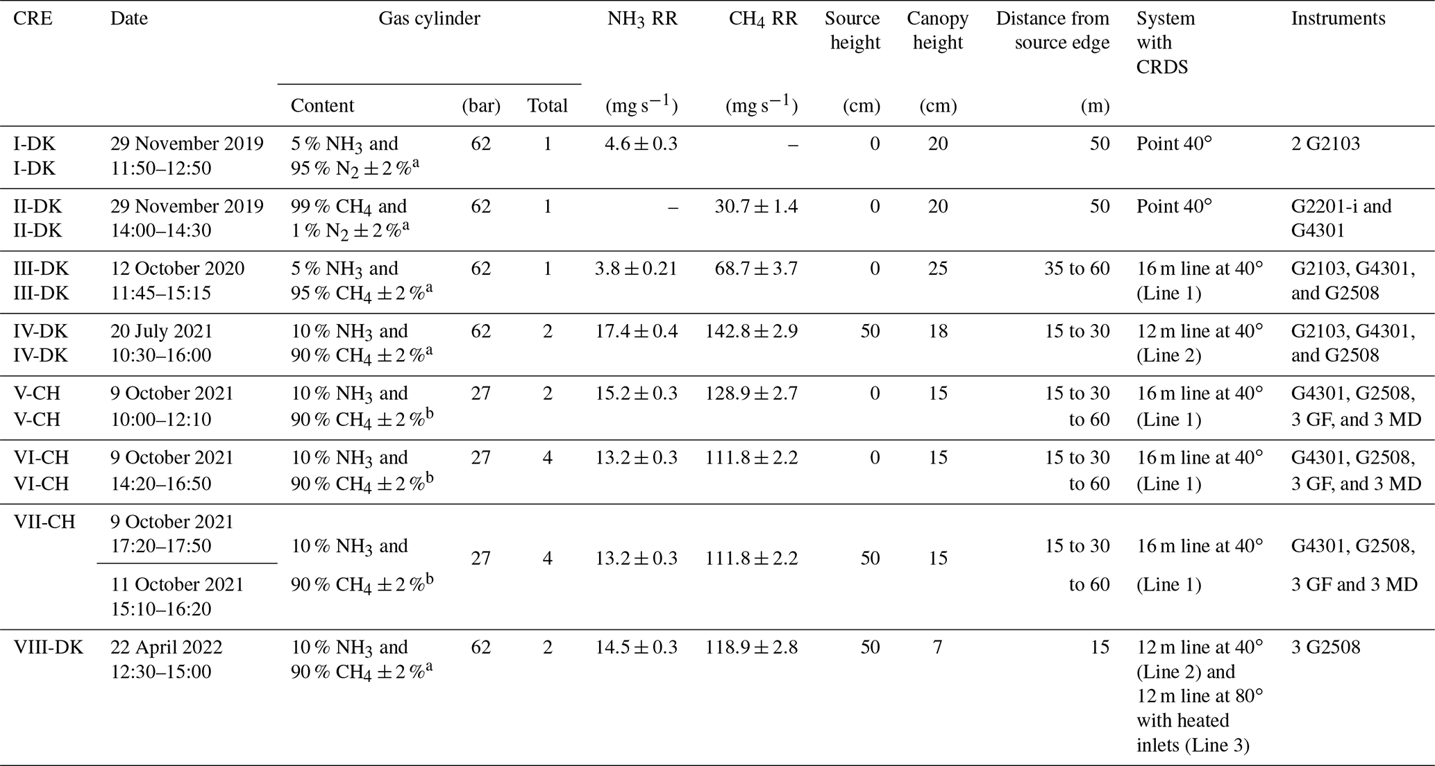
^a Air Liquide, Horsens, Denmark. ^b Carbagas, Bern, Switzerland.

2.2 Instrumentation

In this study, different models of cavity ring-down spectroscopy (CRDS) analyzers from Picarro (Picarro Inc., Santa Clara, CA, USA) were used to measure up- and downwind NH₃ and CH₄ concentration (Table 1). Model G2201-i and model G4301 measure CH₄ concentration, G2103 measures NH₃ concentration, and G2509 measures CH₄ and NH₃ simultaneously. The CRDS is a closed-path analyzer with continuous absorption that measures concentrations at approximately 0.5 Hz. The CRDS analyzer consists of a laser and an optical cavity chamber with highly reflective mirrors, which give an effective path length of several kilometers. The light is absorbed in the cavity, and the decay of light intensity is called the ring-down time, which is directly related to the concentration of the specific compound. It has been frequently used to study agricultural emissions (e.g., Kamp et al., 2021; Pedersen et al., 2020; Kamp et al., 2019; Sintermann et al., 2011). Calibration of these CRDS instruments is conducted using a certified standard gas and a dilution system with NH₃-free air before each release. Mass flow controllers (Bronkhorst EL-FLOW, Ruurlo, the Netherlands) were used to obtain a range of desired concentrations in all calibrations. The standard gas contained 10±0.31 ppm NH₃ (Air Liquide, Horsens, Denmark) and 100±2 ppm CH₄ (Air Liquide, Horsens, Denmark). Calibration showed high linearity of the instruments with R²=1. The CRDS instruments used pairwise for upwind and downwind measurements agreed within ±5 %, and no correction of the instruments was therefore done; see Figs. S5 and S6 in the Supplement.

In experiments V-CH to VII-CH, the downwind CH₄ concentration was measured with three GasFinder3 analyzers (GF3, Boreal Laser Inc., Edmonton, Canada) and the downwind NH₃ concentration with three miniDOAS instruments (Sintermann et al., 2016). The GF3 analyzer is an open-path tunable diode laser device that measures line-integrated CH₄ concentrations over path lengths of 5 to 500 m (i.e., single path length between sensor and retroreflector) with a temporal resolution of 0.3 to 1 Hz. The retroreflectors used in the experiments were equipped with seven corner cubes, suitable for path lengths around 50 m. The GasFinder devices have been widely used to measure emissions from different types of agricultural sources with the IDM (Bühler et al., 2021; McGinn et al., 2019; VanderZaag et al., 2014; Harper et al., 2010; Flesch et al., 2007). The performance of the GF3 instruments is discussed in detail by Häni et al. (2021). The GF3 instruments were intercompared with the calibrated CRDS instrument by measuring ambient concentrations over at least 1 d and corrected accordingly. The applied corrections were $c=c_{\mathrm{GF}}+\mathrm{0.14}$, $c=c_{\mathrm{GF}}+\mathrm{0.22}$, and $c=c_{\mathrm{GF}}+\mathrm{0.12}$ for the GF3 placed 15, 30, and 60 m from the source, respectively.

The miniDOAS instrument is an open-path device that measures NH₃, NO, and SO₂ in the UV region between 190 and 230 nm based on the differential optical absorption spectroscopy (DOAS; Platt and Stutz, 2008) technique. It provides path-averaged concentrations for path lengths between 15 and 50 m, with around 10 to 20 scans per second averaged over 1 min. Ammonia emissions from agricultural sources (Kamp et al., 2021; Kupper et al., 2021; Voglmeier et al., 2018) and from an artificial source (Häni et al., 2018) were measured with miniDOAS analyzers. Further details on the instrument is given in Sintermann et al. (2016). The miniDOAS instruments were intercompared with the calibrated CRDS instrument by measuring ambient concentrations over at least 1 d. The miniDOAS offset concentration from the reference period 8 October 2021 from 15:30 to 17:00 (the time zone for all instances in the text is GMT+1) was added (3.2 µg m⁻³).

2.3 Gas release from an artificial source

The artificial source area had a gas distributor unit at the center, and eight $\mathrm{1}/\mathrm{4}$ in. polytetrafluoroethylene (PTFE) tubes leave the distributor to get a circular shape of the source area. Each tube contained three critical orifices (100 µm diameter, stainless steel, Lenox Laser, USA) in series with a 3 m distance between them. In total, the 24 orifices covered a circular area of 254 m².

Gas was released from a gas cylinder, and the flow was controlled with a mass flow controller (in Denmark: Bronkhorst EL-FLOW; Ruurlo, the Netherlands; in Switzerland: red-y smart controller, Vögtlin Instruments GmbH, Aesch, Switzerland). The source height, the content of the gas cylinders, and the release rate for each experiment are given in Table 1.

2.4 Setup

In the upwind position of all the experiments and in the downwind position of the I-DK and II-DK experiments, the CRDS measured the concentration from a single point 1.5 m above ground through a polytetrafluoroethylene (PTFE) tube that was insulated and heated to approximately 40^∘C. In the rest of the experiments, the CRDS measured downwind concentration from a sampling line system of PTFE tubes (Lines 1 and 2) or polyvinylidene fluoride (PVDF) tubes (Line 3). All tubes were insulated and heated (40 ^∘C or 80 ^∘C). The difference between the point and line-integrated system is the number of positions where the gas sample is taken from. The point system had only one inlet, while the line-integrated had several. Three different versions of the line-integrated system (line) were built and used during this research. In the III-DK, V-DK, VI-CH, and VII-CH experiments, the sampling line system consisted of a 16 m tube with nine inlets, 2 m between each inlet (Line 1). In the IV-DK and VIII-DK experiments, the sampling lines were 12 m long with seven inlets, 2 m between each inlet (Lines 2 and 3). The inlets are made of critical orifices (0.25 mm i.d. for I-DK to VII-CH and 0.5 mm ID for VIII-DK polyetheretherketone (PEEK)) that guarantee uniform flow through each inlet (Lines 1 to 3). In the VIII-DK experiment, the sampling line system including the inlets was heated to 80 ^∘C (Line 3).

Figure 1 shows the position of the source area relative to the sampling position, and the arrow indicates the wind direction during the experiments. The downwind concentrations were measured in one, two, or three distance (Table 1). In the V-CH, VI-CH, and VII-CH, downwind concentrations were measured at the same time at 15, 30, and 60 m distance from the edge of the source with multiple GF3 and miniDOAS instruments; one CRDS instrument was placed 15 m downwind (Fig. 1). The distance between the reflector and the laser and detector of the GF3 and miniDOAS at the downwind position parallel to the CRDS sampling line was also 16 m. For the other two downwind positions the path lengths were 15 and 50 m, respectively. The height of the measurement paths of all the open-path instruments was between 1.2 and 1.5 m. The background concentration of NH₃ was stable with no sources in close vicinity, thus in the three experiments, the average concentration of each instrument 10 min before the release of each experiment was used as the NH₃ upwind concentration for the miniDOAS and the CRDS instruments. In the V-CH, VI-CH, and VII-CH experiments, the measured NH₃ background concentration was 2.7 and 4.1 mg m⁻³ for the miniDOAS and 2.1 and 4.8 mg m⁻³ for the CRDS, respectively. The background concentration for V-CH and VI-CH was the same, since they were carried out on the same day (see Table 1).

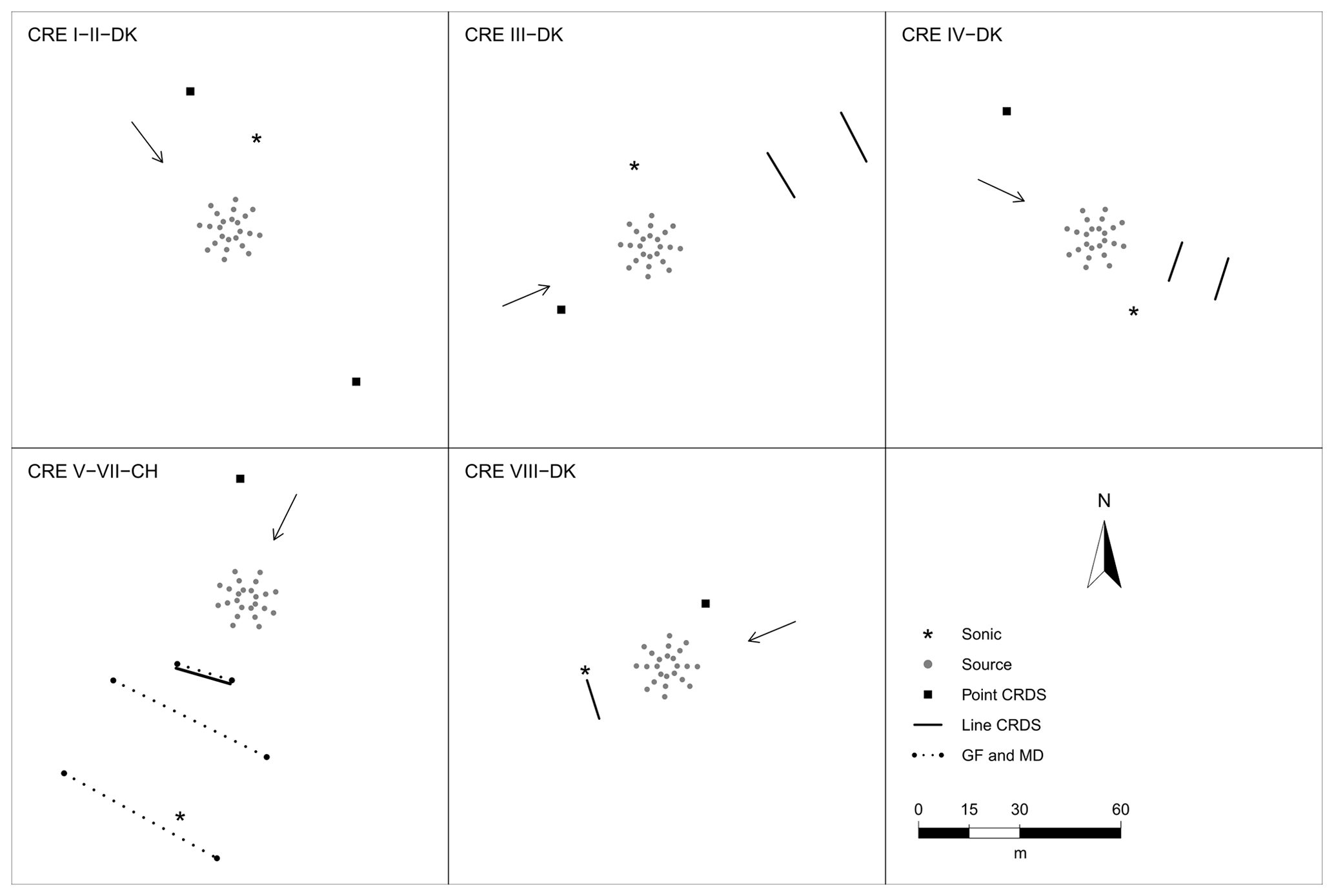
Figure 1 Position of the orifices of the artificial source, ultrasonic anemometer (sonic), and the concentration analyzer used in the eight controlled-release experiments (CRE) of this study. Three types of analyzers have been used: cavity ring-down spectrometer (CRDS), GasFinder (GF), and miniDOAS (MD). The arrow indicates the wind direction during each experiment.

In Denmark, the three wind components were measured at 16 Hz with a 3D ultrasonic anemometer (WindMaster, Gill, Hampshire, UK) at a 1.5 and 1.7 m height. In addition to concentration and wind, air temperature and atmospheric pressure were also measured. In Switzerland, the wind components were measured at 20 Hz with a 3D ultrasonic anemometer (WindMaster, Gill, Hampshire, UK) at a 2 m height. Air temperature and atmospheric pressure were obtained from a meteorological station nearby the experiment site.

A global positioning system (in Denmark: GPS Trimble R10; Sunnyvale, California, USA; in Switzerland: GPS Trimble Pro 6; Sunnyvale, California, USA) was used to record the position of all instruments and the individual critical orifices of the source.

2.5 Inverse dispersion method

The measured gas emission rates (Q) from the artificial source were calculated in 15 min (experiments conducted in Denmark) or 10 min average intervals (experiments conducted in Switzerland) using the R (R Core Team, 2018) package bLSmodelR (https://github.com/ChHaeni/bLSmodelR, last access: 15 December 2022; version 4.3) as described by Häni et al. (2018). The simulation was performed with six million backward trajectories (N) and the source area defined as 24 individual circles of 5 cm radius as described by Häni et al. (2018) with a high-performance computer cluster (PRIME – Programming Rig for Modern Engineering, Aarhus University).

The emissions rate (Q) is proportional to the difference between measured concentration downwind (C_downwind) from the source and the measured background concentration (C_upwind) and the dispersion factor (D):

$$\begin{array}{}\text{(1)}& Q={\displaystyle \frac{C_{\mathrm{downwind}}-C_{\mathrm{upwind}}}{D}}.\end{array}$$

The dispersion factor (D) is calculated as

$$\begin{array}{}\text{(2)}& D={\displaystyle \frac{\mathrm{1}}{N}}\sum _{\mathrm{TDinside}}\left|{\displaystyle \frac{\mathrm{2}}{w_{\mathrm{TD}}}}\right|,\end{array}$$

where N is the number of backward trajectories from the downwind analyzer location. The summation refers to the trajectories touching inside the source area (TDinside), taking the vertical velocity (w_TD) at touchdown into account. The calculation of D includes determination of wind profiles and turbulence statistics that are based on the Monin–Obukhov similarity theory (MOST).

2.6 Surface deposition velocity

Ammonia is a relatively short-lived gas in the atmosphere and can either be chemically converted or subjected to dry or wet deposition. Dry deposition of NH₃ is a complex mechanism that is restricted by both atmospheric dispersion towards and uptake at surfaces (thus, it is correlated to several different conditions indicated by, e.g., wind speed, solar radiation, vegetation reactivity). The dry NH₃ deposition rate is often expressed with a deposition velocity (υ_d). In this study, we model dry deposition as a canopy resistance (“big leaf”) approach where υ_d takes place unidirectionally, and it is calculated with the canopy resistances (Hicks et al., 1987):

$$\begin{array}{}\text{(3)}& {\mathit{\upsilon }}_{\mathrm{d}}={\displaystyle \frac{\mathrm{1}}{R_{\mathrm{a}}+R_{\mathrm{b}}+R_{\mathrm{c}}}},\end{array}$$

where R_a is the aerodynamic resistance, R_b is the quasi-laminar boundary resistance, and R_c is the bulk canopy resistance. Because R_a (the resistance between the concentration measurement height and the notional height z₀) is already included in the bLS model calculations, Eq. (3) can be simplified to represent a surface deposition velocity:

$$\begin{array}{}\text{(4)}& {\mathit{\upsilon }}_{\mathrm{d}}^{*}={\displaystyle \frac{\mathrm{1}}{R_{\mathrm{b}}+R_{\mathrm{c}}}}.\end{array}$$

For each model trajectory calculation, this surface deposition velocity is acting on each touchdown outside the emitting source to provide individual dry deposition fluxes F_d from prevailing touchdown concentration C_TD as

$$\begin{array}{}\text{(5)}& F_{\mathrm{d}}=-{\mathit{\upsilon }}_{\mathrm{d}}^{*}{C}_{\mathrm{TD}}.\end{array}$$

This reduces the modeled trajectory concentration at each touchdown outside the source by

$$\begin{array}{}\text{(6)}& \mathrm{\Delta }{C}_{\mathrm{d}}=C_{\mathrm{TD}}\cdot \left(\exp \left(-{\displaystyle \frac{\mathrm{2}\cdot {\mathit{\upsilon }}_{\mathrm{d}}^{*}}{w_{\mathrm{TD}}}}\right)-\mathrm{1}\right).\end{array}$$

We refer to Häni et al. (2018) for the derivation of the above equation and a thorough explanation of the implementation of the dry deposition algorithm in the bLS model.

In this study, R_b was calculated according to Garland (1977), as a function of the roughness length (z₀), friction velocity (u^*), kinematic viscosity of air (ν), and molecular diffusivity of NH₃ in air $\left({\mathit{\delta }}_{{\mathrm{NH}}_{\mathrm{3}}}\right)$:

$$\begin{array}{}\text{(7)}& R_{\mathrm{b}}={\displaystyle \frac{\mathrm{1.45}{\left(\frac{z_{\mathrm{0}}{u}_{*}}{\mathit{\nu }}\right)}^{\mathrm{0.24}}{\left(\frac{\mathit{\nu }}{{\mathit{\delta }}_{{\mathrm{NH}}_{\mathrm{3}}}}\right)}^{\mathrm{0.8}}}{u^{*}}}.\end{array}$$

Regarding R_c, it is related to the chemical characteristics of the studied gas and the characteristics of the leaf (e.g., type, size). There are different models to calculate R_c. Due to the complexity and the uncertainty of the determination of the resistance, R_c was calculated following the same procedure as by Häni et al. (2018) with the bLSmodelR. It was assumed that $Q_{\mathrm{bLS}}/Q<\mathrm{1}$ was solely due to dry deposition. A similar approach is used here, where 12 values of R_c from 0 to 500 s m⁻¹ were tested in the bLS model that includes ammonia deposition to estimate the R_c, giving $Q_{\mathrm{bLS}}/Q=\mathrm{1}$ in all intervals. This was done with linear interpolation between the two points closest to $Q/Q=\mathrm{1}$. Using this estimated R_c and the calculated R_b value for each interval, ${\mathit{\upsilon }}_{\mathrm{d}}^{*}$ was estimated for all intervals with all instruments. The ${\mathit{\upsilon }}_{\mathrm{d}}^{*}$ values are compared to previously reported values for NH₃.

Another approach for calculating the R_c is with an empirical equation, which will be used for calculating values for ${\mathit{\upsilon }}_{\mathrm{d}}^{*}$. These calculated values will be compared to the values obtained with the bLS model. It is assumed that R_c is unidirectional and equal to the sum of the stomatal resistance R_s and the cuticular resistance R_w; see Eq. (6).

$$\begin{array}{}\text{(8)}& {\displaystyle \frac{\mathrm{1}}{R_{\mathrm{c}}}}={\displaystyle \frac{\mathrm{1}}{R_{\mathrm{s}}}}+{\displaystyle \frac{\mathrm{1}}{R_{\mathrm{w}}}}\end{array}$$

The stomatal resistance R_s is calculated with equation Eq. (7) (Wesely, 2007):

$$\begin{array}{}\text{(9)}& R_{\mathrm{s}}=R_{\mathrm{s}(min)}[\mathrm{1}+\left({\displaystyle \frac{\mathrm{200}}{SR+\mathrm{0.1}}}\right){]}^{\mathrm{2}}{\displaystyle \frac{\mathrm{400}}{T_{\mathrm{s}}\left(\mathrm{40}-T_{\mathrm{s}}\right)}},\end{array}$$

where R_s(min) is the minimum bulk canopy R_s for water vapor that is assumed to be equal to 250 s m⁻¹ (Lynn and Carlson, 1990), SR is the solar radiation, and T_s is the soil temperature.

The cuticular resistance is calculated with Eq. (8) (Massad et al., 2010):

$$\begin{array}{}\text{(10)}& R_{\mathrm{w}}={\displaystyle \frac{R_{\mathrm{w}}\left(min\right)e^{a(\mathrm{100}-\mathrm{RH})}{e}^{\mathrm{0.15}T}}{{\left(\text{LAI}\right)}^{\mathrm{0.5}}}},\end{array}$$

where R_w(min) is the minimum cuticular resistance, a is an empirical factor, RH is the relative humidity, T is the air temperature, and LAI is the leaf area index. The parameters R_w(min) (10 s m⁻¹), a (0.110), and LAI (2 m² m⁻²) were obtained from Massad et al. (2010), Table 1.

3 Results and discussion

3.1 Recovered fractions of ammonia and methane

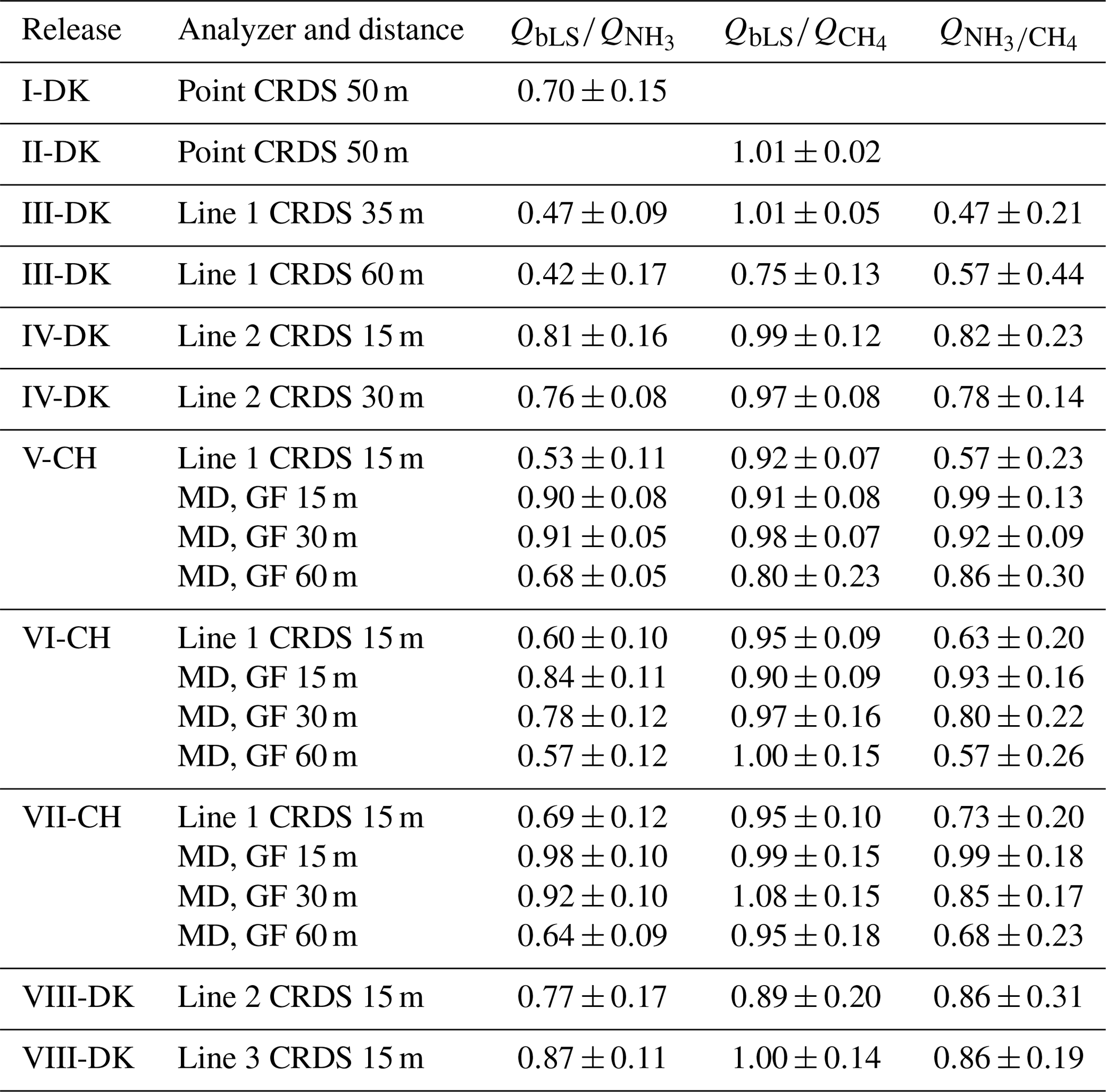
The accuracy of the bLS model is evaluated by the recovered NH₃ and CH₄ fractions, $Q_{\mathrm{bLS}}/Q$, and the standard deviation ${\mathit{\sigma }}_{Q_{\mathrm{bLS}}/Q}$ for all the releases without taking NH₃ deposition into account. In all experiments except I-DK and II-DK (Table 1), NH₃ and CH₄ were released simultaneously. The use of these two gases gives us the additional opportunity to assess potential loss of NH₃ downwind from the source by deposition or gas-to-particle conversion, processes that will not occur for CH₄ due to its inertness. As the average of all releases and measurement systems, the CH₄ recovery rate was 0.95±0.08 (n=19) (Fig. 4). This recovery is similar to 0.93±0.14 (n=8) observed by Gao et al. (2008) with a different controlled release configuration and ground-level sources. There was more variation in the recovery of NH₃, with an average of 0.66±0.15 (n=10) for all the releases with the line-integrated system. However, the improved sampling lines (Lines 2 and 3) placed at 15 m downwind from the source had an average recovery of 0.82±0.05 (n=3) for NH₃ (Fig. 2). Under comparable conditions, the NH₃ recovery rate obtained with the miniDOAS (MD) was 0.91±0.07 (n=3). Häni et al. (2018) observed almost the same recovered fraction, 0.91±0.12, at 15 m from the edge of the source with the MD. The recovery rates of all experiments in this study are shown in Fig. 2, whereas climate conditions such as wind direction, friction velocity u_∗, air temperature, relative humidity (RH), soil temperature, and solar radiation (SR) from each experiment are presented in Table S2 in the Supplement. In addition, the average of the recovery fraction rates of both gases and their relation in each release are shown in Table 2. I-DK and II-DK were conducted during cold conditions (∼5 ^∘C) with RH ranging from 65 % to 71 %, whereas IV-DK and VIII-DK were conducted in warm conditions (14–18 ^∘C) with RH between 48 % and 63 %. The other releases were conducted under moderate temperature conditions (10–13 ^∘C) with RH between 39 % and 89 %.

Additional information on the atmospheric conditions, weather conditions, and recovery fraction rates for each average time interval for each release is shown in Table S1.

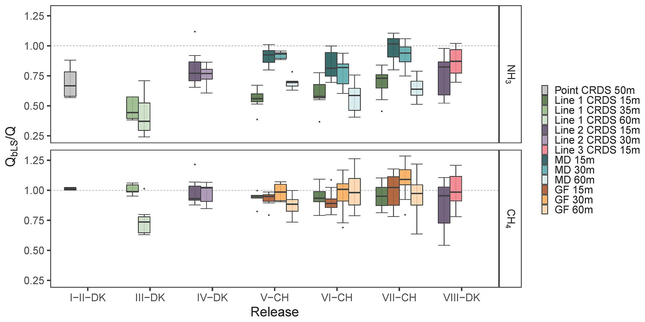
Figure 2 The recovered fractions $Q_{\mathrm{bLS}}/Q$ of ammonia and methane from each release and analyzer. The downwind distance from the source to the analyzer is indicated in the legend. Line 1 had a length of 16 m, and it was heated to 40 ^∘C. Line 2 had the same temperature as Line 1, but it was 12 m long. Line 3 had the same length as Line 2 but was heated to 80 ^∘C. Error bars represent the standard deviation.

Table 2 Average of the recovery fractions $Q_{\mathrm{bLS}}/Q$ of ammonia and methane for each release and analyzer with standard deviation. Lines 1 to 3 are described in the Fig. 2 caption.

3.2 Sampling systems for closed-path measurement

Three different CRDS sampling line systems have been used from III-DK to VIII-DK. The difference between the lines was the length and the heating temperature. Line 1 had a length of 16 m, and it was heated to 40 ^∘C. Line 2 had the same temperature as Line 1, but it was 12 m long. Line 3 had the same length as Line 2 but was heated to 80 ^∘C, and the critical orifices have a higher inflow than Lines 1 and 2 (see Sect. 2.4 Setup). We expect that decreasing the length and increasing the heating temperature of the line will improve $Q_{\mathrm{bLS}}/Q$ for NH₃ (no expected effect for CH₄) by avoiding adsorption and reducing the response time in the sampling line.

Line 1 was used with the source at ground level and elevated (Table 1), whereas the other two lines only with the source elevated. When the source was at ground level, Line 1 had a recovery rate ranging from 0.42±0.17 to 0.60±0.10 and from 0.75±0.13 to 1.01±0.05 for NH₃ and CH₄, respectively. The lowest and the highest NH₃ recovery rate of Line 1 are directly related to the furthest (60 m) and the shortest (15 m) downwind distance measurement from the source. In addition, the standard deviation ${\mathit{\sigma }}_{Q_{\mathrm{bLS}}/Q}$ at the furthest position is higher than at the closest position, which is in accordance with the results from Häni et al. (2018). High uncertainty of the $Q_{\mathrm{bLS}}/Q$ is related to a smaller difference in concentration between downwind and background concentrations and due to smaller D values (Häni et al., 2018). This is also the reason for the low CH₄ recovery rate of Line 1 in III-DK at 60 m (0.75±0.13); downwind concentration is only 4 %–10 % higher than upwind concentrations, since this is one of the lowest CH₄ release rates (Table 1). This is in line with Coates et al. (2021), who observed that the bLS model underestimated 49 % of CO₂ released at 50 m fetch distance, partially because the measured downwind concentration was close to the background level. Therefore, in this study, the accuracy of Q_bLS is mainly influenced by the uncertainty of the concentration measurement, hence the downwind distance is limited by the properties of the gas analyzers and the size of the emission strength of the source. This means the system can be limited in use if the emission source has a large height and low emission strength where, as a rule of thumb, measurements should be conducted at a distance from the source at least 10 times the height of the source (Harper et al., 2011).

In VII-CH, Line 1 was used with the source elevated and had a recovery rate of 0.69±0.12 for NH₃ and 0.95±0.10 for CH₄. Line 2 had a numerically higher recovery rate than Line 1, ranging from 0.76±0.08 to 0.81±0.16 and from 0.89±0.20 to 0.99±0.12 for NH₃ and CH₄, respectively, in IV-DK and VIII-DK. The length of the line appears to affect the NH₃ recovery rate; this might be due to the increased surface area that NH₃ can adsorb to, and there is a lower flow in each of the critical orifices that decreases the response time of the system (Shah et al., 2006; Vaittinen et al., 2014). Looking at the measured NH₃ rates over time (Fig. 3), higher emissions are reached with Line 3 for the first hour, indicating a faster time response compared to Line 2. However, after an hour there was not a clear difference between the lines. The results indicate that increasing the sampling line temperature to 80 ^∘C had a positive effect on the recovery, which reached 87 % at a distance of 15 m. From the data obtained by the open-path analyzer (MD), we can conclude that deposition can cause a reduction in recovery in the order of 2 %–16 % (Fig. 2). Thus, the recovery obtained with the improved line (Line 3) approaches the recovery obtained with the open-path analyzer. It should be noted that a direct comparison between Line 3 and the open-path analyzer (MD) has not been made, and further improvement can still be suggested for the CRDS sampling line system. Specifically, increasing the flow through the sampling line and critical orifices will reduce NH₃ adsorption in the tubing material. However, similar flow rates through the sampling orifices in the sampling line must still be ensured.

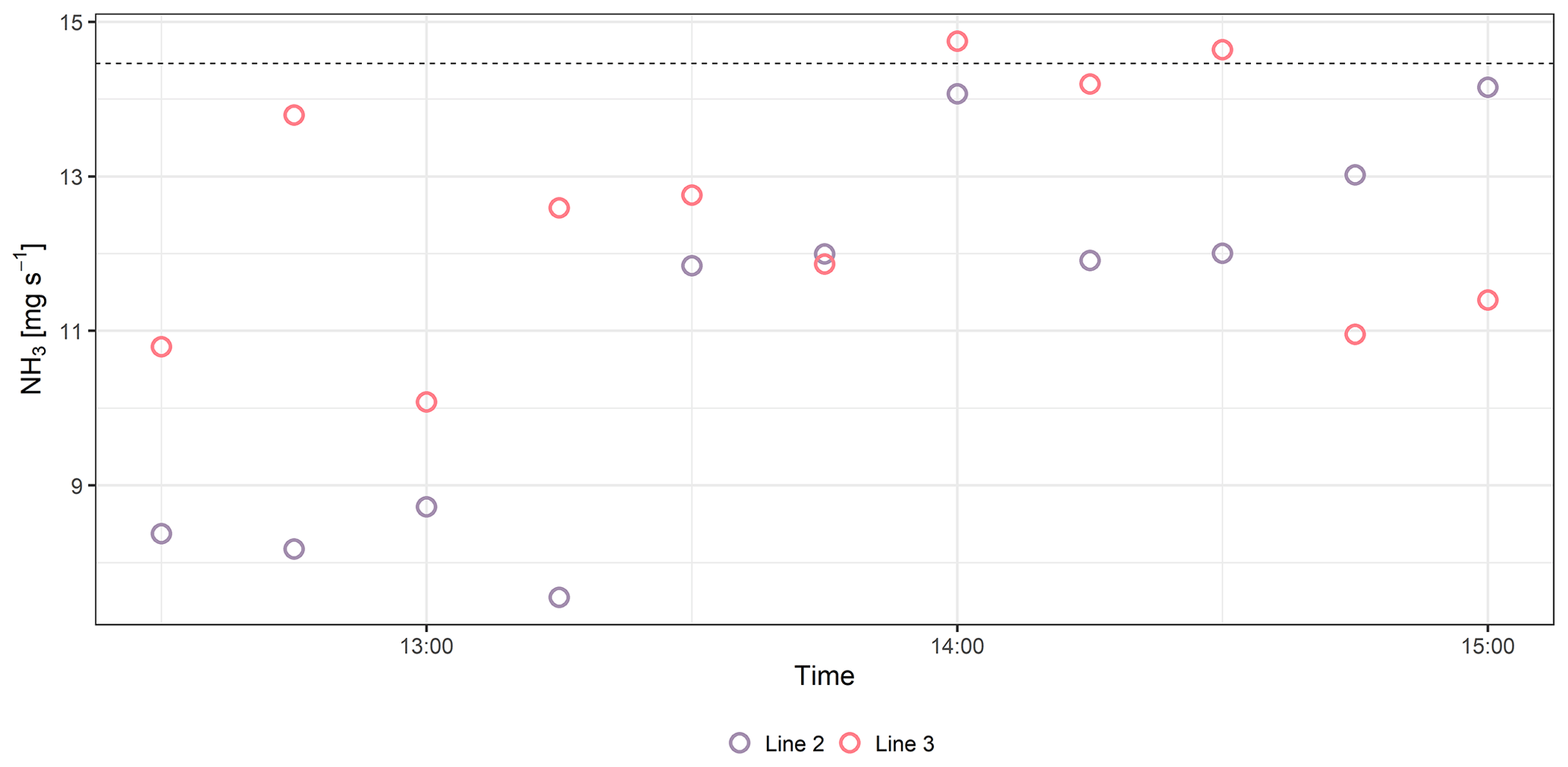
Figure 3 Ammonia (NH₃) fluxes measured with Line 2 and Line 3 in 10 min interval averages in VIII-DK.

The point CRDS system had a recovery rate of 0.70±0.22 and 1.01±0.05 for NH₃ and CH₄, respectively. The benefit of the point CRDS system is mainly that increasing the flow in the tubing is less limited, since there are no critical orifices for which equal flow must be maintained. However, comparing point and line CRDS systems to the modeled concentration distribution (Fig. 4), the line-integrated measurement system covers a larger part of the emission plume from the source in a higher wind direction range. In addition, a line-integrated measurement system can reduce uncertainty in the IDM (Flesch et al., 2004), since it is less sensitive to error in the measured wind direction. This is in accordance with Ro et al. (2011), who observed an almost double recovery value of a line-integrated measurement system for CH₄ compared to a point measurement system using a photoacoustic gas monitor.

Figure 4 Contours of the modeled concentration distribution (C_bLS) for CRE I-DK, CRE III-DK, and CRE IV-DK.

3.3 Open-path measurement systems

The recovery rates for the GFs (CH₄) ranged from 0.87±0.10 to 1.08±0.15. In V-CH to VII-CH, the corresponding standard deviation ${\mathit{\sigma }}_{Q_{\mathrm{bLS}}/Q}$ of GF 15 m varies from 0.07 to 0.18, while Line 1 (placed parallel to GF 15 m) ranges from 0.06 to 0.10. These standard deviations ${\mathit{\sigma }}_{Q_{\mathrm{bLS}}/Q}$ are comparable with those measured by Gao et al. (2009) (1.03±0.16).

In V-CH and VI-CH (source at ground), the MDs (NH₃) had recovery rates ranging from 0.57±0.12 to 0.93±0.03. In VII-CH, MDs exhibit higher recoveries ranging from 0.64±0.09 to 0.98±0.10, since the source was elevated. Generally, it is recommended to do a release experiment above ground level to reduce the probability of deposition close to the release area (McBain and Desjardins, 2005). As expected, the recovery rate decreased with downwind distance of the sampling position due to NH₃ deposition, which will be evaluated in Sect. 3.4. Comparing MD at 15 m and Line 1 (placed in parallel) in V-CH to VII-CH (Fig. 2), the recovery rates are higher for MD. The highest difference between MD and Line 1 was in V-CH, where there was the highest RH (87 %). However, there are no clear patterns explaining the difference between emissions from the different measurement systems based on atmospheric conditions (Fig. S2). Although the improved recovery with Line 2 (0.81±0.16) and Line 3 (0.87±0.11) in IV-DK and VIII-DK could be influenced by the warmer conditions and solar radiation (Table S2), it is plausible that the line improvements caused the increase. An increased flow through the orifices and higher temperature of the sampling line will lead to less NH₃ adsorption, thereby getting a better recovery from the release.

These results show the advantage of an open-path instrument compared to a closed-path instrument to measure NH₃ emissions (Fig. 2), since open-path avoids prolonged response caused by the adsorption of NH₃ to sampling materials (Shah et al., 2006; Vaittinen et al., 2014). However, quality assurance is more challenging for open-path instruments, because the use of a closed gas cell for calibration with a certified gas standard is tedious and means that the instrument setup deviates significantly from field measurement (DeBruyn et al., 2020). Intercomparison to a reference method (as an alternative to gas standard calibration) may also introduce uncertainties (Häni et al., 2021). In addition, the closed-path system presented in this study (line CRDS) is more flexible with respect to moving the sampling line around the source depending on the predominant wind direction. This is particularly important in areas with frequently changing wind direction.

3.4 Surface deposition velocity

The corresponding surface deposition velocities (${\mathit{\upsilon }}_{\mathrm{d}}^{*})$ required to have a recovery rate $Q_{\mathrm{bLS}}/Q=Q_{{\mathrm{CH}}_{\mathrm{4}}}$ are presented in Fig. 5. This approach assumes a recovery equals to the measured $Q_{{\mathrm{CH}}_{\mathrm{4}}}$ for each of the measurement systems when taking deposition into account, which is not completely correct for closed-path sampling. In the following, therefore, we refer to deposition velocity required to achieve $Q_{\mathrm{bLS}}/Q=Q_{{\mathrm{CH}}_{\mathrm{4}}}$ as the apparent deposition velocity (${\mathit{\upsilon }}_{\mathrm{ad}}^{*})$. This is included to provide data on deposition velocities for ammonia for which data are currently very limited. The recovery rates observed in Fig. 2 show that the MD performed best, whereas lower $Q_{\mathrm{bLS}}/Q$ were seen in the sampling lines, thus the lowest ${\mathit{\upsilon }}_{\mathrm{ad}}^{*}$ is expected from MD. Additional information of R_c and ${\mathit{\upsilon }}_{\mathrm{ad}}^{*}$ for each time interval in each experiment is shown in Table S1. The apparent surface deposition velocities ranged from 0.2 to 1.8 cm s⁻¹ for open-path data and from 0.2 to 4.2 cm s⁻¹ for the line sampling. Häni et al. (2018) reported ${\mathit{\upsilon }}_{\mathrm{ad}}^{*}$ in the range from 0.3 to 1.1 cm s⁻¹. In all the releases where downwind concentrations were measured at different positions, ${\mathit{\upsilon }}_{\mathrm{ad}}^{*}$ appears to increase with distance. For example, in VI-CH, ${\mathit{\upsilon }}_{\mathrm{ad}}^{*}$ is 0.3±0.1, 0.7±0.4, and 1.1±0.5 cm s⁻¹ at 15, 30, and 60 m, respectively. The reason for this increase with distance is presently unclear and should be investigated further.

In V-CH, VI-CH, and VII-CH, ${\mathit{\upsilon }}_{\mathrm{ad}}^{*}$ from Line 1 are 4.9, 4.3, and 4.3 times higher than MD at 15 m. As expected ${\mathit{\upsilon }}_{\mathrm{ad}}^{*}$ was higher for Line 1, as the $Q/Q$ was lower for Line 1 compared to MD in these experiments. Comparing the apparent deposition velocities from these experiments show comparable values for Lines 2 and 3 but higher values for Line 1, i.e., Line 1 (VII-CH) had ${\mathit{\upsilon }}_{\mathrm{ad}}^{*}$ of 1.7±0.4, whereas Lines 2 and 3 (VIII-DK) had ${\mathit{\upsilon }}_{\mathrm{ad}}^{*}$ of 1.4±0.4 and 1.2±0.6 cm s⁻¹, respectively, when measuring 15 m from the elevated source. During VII-CH and VIII-DK the temperature differed with 1 ^∘C, and the relative humidity was approximately the same, but wind speed and solar radiation differed (Table S2).

Figure 5 Corresponding apparent surface deposition velocities (${\mathit{\upsilon }}_{\mathrm{ad}}^{*})$ required to have a recovery rate $Q_{\mathrm{bLS}}/Q$ closest to one in all the releases. The error bars represent the standard deviations. All values are shown in Table S1.

Many factors affect the deposition velocity, but it is possible to calculate ${\mathit{\upsilon }}_{\mathrm{ad}}^{*}$ from empirical models as explained previously (see Sect. 2.6). Figure 6 shows ${\mathit{\upsilon }}_{\mathrm{ad}}^{*}$ for MDs in V-CH, VII-CH, and VIII-CH compared to ${\mathit{\upsilon }}_{\mathrm{ad}}^{*}$ calculated with the empirical models (Eqs. 3–8). Using the empirical models, ${\mathit{\upsilon }}_{\mathrm{ad}}^{*}$ varies from 0.13 to 1.02 cm s⁻¹, increasing with the relative humidity (87 %, 76 %, and 52 % RH in V-CH, VI-CH, and VII-CH, respectively). The difference between the two ways of estimating ${\mathit{\upsilon }}_{\mathrm{ad}}^{*}$ is not surprising, since (i) bLS-derived deposition may be influenced by methodological uncertainties and therefore deviate from true deposition, and (ii) calculated resistances are associated with uncertainties due to estimations of physical parameters. In addition, an artificial source most likely will have higher ${\mathit{\upsilon }}_{\mathrm{d}}^{*}$ than what is expected from a typical agricultural source (Häni et al., 2018). This is expected, because an artificial source with discrete outlets located near the ground will have a larger deposition close to the release, because the ground has a high capacity for NH₃ sorption. On the contrary, a constantly and homogeneously emitting source (e.g., storage tank or manure pile) is not expected to have any significant deposition within the source. This is seen with the higher ${\mathit{\upsilon }}_{\mathrm{ad}}^{*}$ values found in these experiments compared to the calculated values with the empirical models. The height of the source might also have an influence on ${\mathit{\upsilon }}_{\mathrm{ad}}^{*}$. This is indicated by the lowest ${\mathit{\upsilon }}_{\mathrm{ad}}^{*}$ in VII-CH, where the source was elevated compared to V-CH and VI-CH, where the gas was released on the surface. Placing the source above ground level will reduce the obstacles (crop on the field) for gas dispersion, reducing surface deposition. However, the bLS model does not consider the height of the source. For example, evaluating emissions from the application of liquid animal manure (ground-level source) or a dairy housing (elevated source) will have different ${\mathit{\upsilon }}_{\mathrm{ad}}^{*}$.

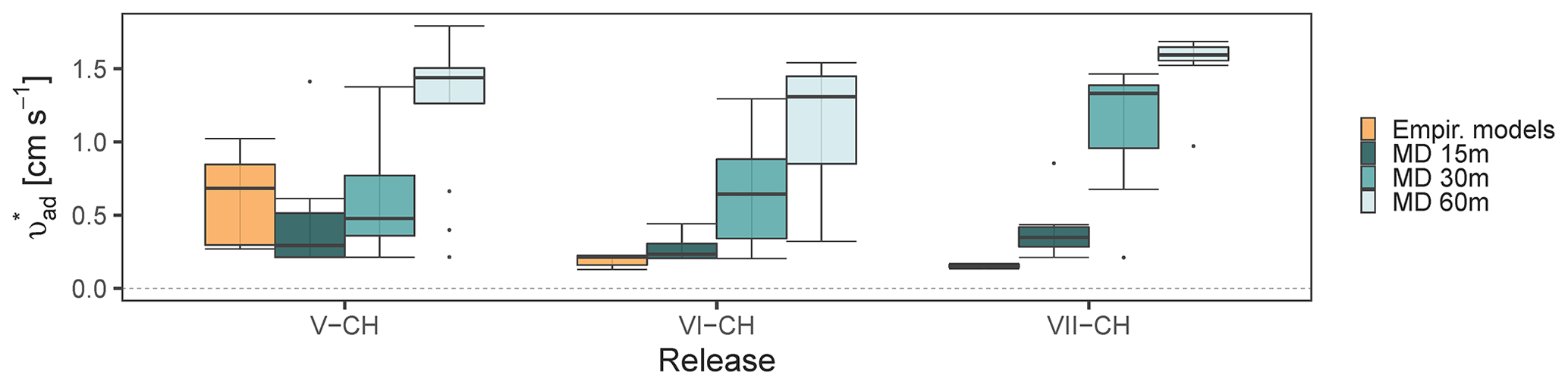
Figure 6 Corresponding apparent surface deposition velocities (${\mathit{\upsilon }}_{\mathrm{ad}}^{*}$) required to have a recovery rate $Q_{\mathrm{bLS}}/Q$ closest to one for miniDOAS (MD) in release V-CH, VI-CH, and VII-CH and ${\mathit{\upsilon }}_{\mathrm{ad}}^{*}$ calculated with an empirical model.

3.5 Uncertainties and sensitivity analysis

The line-integrated concentration measurement systems with a CRDS analyzer (Lines 1 to 3; excluding one value at 60 m) had an average recovery rate of CH₄ of 96±4 % (1 standard deviation, n=8) (see also Table 2). Based on this, it is concluded that the method is not biased with respect to CH₄. The overall precision of CH₄ concentration measurements observed for the three versions of the line ranged from 4 % to 22 % at a 15 m distance (see Table 2). The equivalent precision for NH₃ concentration measurements was between 13 % and 23 % (Table 2) for the improved sampling lines (Lines 2 and 3) at a 15 m distance (CRE IV and CRE VIII). The 9 % difference between NH₃ recovery rates for MD (CRE V-CH–VII-CH) and for Lines 2 to 3 at a 15 m distance is assessed to represent the sampling line adsorption bias related to the line-integrated system under the best conditions (improved sampling lines and moderate to warm temperatures). The most relevant factors affecting the uncertainties are the determination of the wind direction offset, canopy height, and downwind concentration analyzer height. Furthermore, the accuracy of the concentration measurements and data filtering criteria related to the meteorological conditions (e.g., Flesch et al., 2005) are other important factors that influence the uncertainty of the measurement. It would require a comprehensive study to evaluate the contributions of these parameters, which is not in the scope of this study. Therefore, only sensitivity analyses of the wind direction offset and the sensor height are included below. The individual uncertainty contributions would be lumped into the overall precision and bias mentioned above.

A sensitivity analysis of two input parameters for the bLS model was based on the resulting $Q/Q$ ratio when changing the inlet height of the analyzer and the wind direction offset compared to the valid measured values in release VIII-DK. This was done for 11 fluxes in average intervals of 15 min, where all emissions were estimated again with the bLS model. For the assessment of the influence of the input for the measurement height all other variables were kept constant. Likewise, for the influence of the wind direction, all other variables were kept constant, while the wind direction offset was changed. The results are presented in Fig. S4, where it can be seen that $Q/Q$ was most sensitive to the changes in wind direction offset, stressing the importance of the true offset in wind direction. Therefore, the wind direction must be thoroughly evaluated for the accuracy of emission estimation, since more or less trajectories have touchdowns inside the source area for the dispersion factor (Eq. 2). In addition, the uncertainty of the $Q/Q$ ratio increases as wind direction offset increases. The emission estimation accuracy from point systems is more sensitive to error in the measured wind direction (Flesch et al., 2004).

The accuracy and precision of the emission estimation also depend on the detection limits of the concentration sensor analyzer, especially when the downwind concentration is close to the background level, as it was shown previously (see Sect. 3.2). Therefore, it is recommended to conduct concentration and turbulence measurements not far from the source but a minimum of 10 times the source height according to Harper et al. (2011) at a known height to reduce the uncertainty of the calculated emission rates.

4 Conclusion

For CH₄, the average recovery rate for all releases was 0.95±0.08, which demonstrates that line-averaged measurement with a closed-path analyzer is comparable to an open-path system for inert gases. Under comparable conditions, average recovery rates of 0.82±0.05 (n=3) and 0.91±0.07 (n=3) for NH₃ and 0.94±0.02 (n=3) and 0.93±0.05 (n=3) for CH₄ were obtained with the closed-path and open-path line-integrated system, respectively. The implementation of the new method presented in this study will enable measurement of fluxes of multiple gases from different types of sources and evaluate the effects of mitigation strategies on emissions. In addition, this method allows for continuous online measurements that resolve temporal variation in NH₃ emissions and the peak emissions of CH₄. It is stressed that the wind direction must be thoroughly evaluated for the accuracy of emission estimation with the bLS model.

A significant fraction of the emitted NH₃ is deposited near the source. Consequently, including the deposition algorithm in the bLS model will have less bias in the emission evaluation at ground-level sources (e.g., application of liquid animal manure) compared to elevated sources (e.g., slurry tank). The present study shows that the estimated deposition velocities are in the same order of magnitude in all the releases with some variation across the different approaches (instrument, distance, method).