Optimization of a Picarro L2140-i cavity ring-down spectrometer for routine measurement of triple oxygen isotope ratios in meteoric waters

The demanding precision of triple oxygen isotope (Δ¹⁷O) analyses in water has restricted their measurement to dual-inlet mass spectrometry until the recent development of commercially available infrared laser analyzers. Laser-based measurements of triple oxygen isotope ratios are now increasingly performed by laboratories seeking to better constrain the source and history of meteoric waters. However, in practice, these measurements are subject to large analytical errors that remain poorly documented in scientific literature and by instrument manufacturers, which can effectively restrict the confident application of Δ¹⁷O to settings where variations are relatively large (∼ 25–60 per meg). We present our operating method of a Picarro L2140-i cavity ring-down spectrometer (CRDS) during the analysis of low-latitude rainwater where confidently resolving daily variations in Δ¹⁷O (differences of ∼ 10–20 per meg) was desired. Our approach was optimized over ∼ 3 years and uses a combination of published best practices plus additional steps to combat spectral contamination of trace amounts of dissolved organics, which, for Δ¹⁷O, emerges as a much more substantial problem than previously documented, even in pure rainwater. We resolve the extreme sensitivity of the Δ¹⁷O measurement to organics through their removal via Picarro's micro-combustion module, whose performance is evaluated in each sequence using alcohol-spiked standards. While correction for sample-to-sample memory and instrumental drift significantly improves traditional isotope metrics, these corrections have only a marginal impact (0–1 per meg error reduction) on Δ¹⁷O. Our post-processing scheme uses the analyzer's high-resolution data, which improves δ²H measurement (0.25 ‰ error reduction) and allows for much more rich troubleshooting and data processing compared to the default user-facing data output. In addition to competitive performance for traditional isotope metrics, we report a long-term, control standard root mean square error for Δ¹⁷O of 12 per meg. Overall performance (Δ¹⁷O error of 6 per meg, calculated by averaging three replicates spread across distinct, independently calibrated sequences) is comparable to mass spectrometry and requires only ∼ 6.3 h per sample. We demonstrate the impact of our approach using a rainfall dataset from Uganda and offer recommendations for other efforts that aim to measure meteoric Δ¹⁷O via CRDS.

1 Introduction

The stable isotopic composition of water was among the first applications of isotope ratio mass spectrometry (Dansgaard, 1964; Epstein and Mayeda, 1953) and continues to be a critically useful tool for studying the hydrologic cycle (Bowen et al., 2019; Gat, 1996). The most common form of water, ¹H${}_{\mathrm{2}}^{\mathrm{16}}$O, is measured as a ratio against its heavier, singly substituted isotopologues: ²H¹H¹⁶O, ¹H${}_{\mathrm{2}}^{\mathrm{17}}$O, and ¹H${}_{\mathrm{2}}^{\mathrm{18}}$O. Historically, the ²H : ¹H and ¹⁸O : ¹⁶O variations, reported as δ²H and δ¹⁸O, respectively, have been the primary targets for isotopic analysis. More recently, ¹⁷O : ¹⁶O variations, especially in tandem with ¹⁸O : ¹⁶O, have found applications as a new secondary measurement complementary to deuterium excess (d-excess = δ²H − 8 × δ¹⁸O) capable of tracing a range of processes, including atmospheric vapor formation conditions (Uechi and Uemura, 2019), mixing of differentially evaporated waters (Surma et al., 2018; Voigt et al., 2021), raindrop re-evaporation (Landais et al., 2010), and others (Aron et al., 2021). The coupled variations of the triple oxygen isotope system, calculated relative to a reference slope and referred to in the literature as ¹⁷O excess or Δ¹⁷O (hereafter Δ¹⁷O), are interpreted at the per meg (10⁶ or parts per million) level rather than the typical per mil level (10³, ‰, or parts per thousand). Although multiple formulations exist, throughout this paper we use log transformation of the primary oxygen isotope ratios and an empirical global reference slope of 0.528 (Aron et al., 2021; Luz and Barkan, 2010); see Aron et al. (2021) for a review of the reference slope choices.

The precision required to measure Δ¹⁷O within the range of natural variation was first developed using dual-inlet isotope ratio mass spectrometry (DI-IRMS) after conversion of H₂O to O₂ (Barkan and Luz, 2005). Later, isotope ratio infrared laser spectroscopy (IRIS) instruments were developed to perform triple oxygen isotope measurements without prior conversion of water to other species (Berman et al., 2013; Steig et al., 2014). Compared to DI-IRMS, IRIS instruments cost substantially less, require less operator expertise, and perform their analyses without any modification of the original sample. Since the inception of IRIS techniques in the 2000s, the primary advantages of DI-IRMS have been improved precision (Wassenaar et al., 2018) and insensitivity to organic contamination (West et al., 2010).

The Picarro L2140-i is a cavity ring-down IRIS designed to measure the near-infrared absorption of the four previously mentioned isotopologues of water and thus the Δ¹⁷O parameter. The L2140-i is distinguished from prior models by the inclusion of a second laser (required for ¹⁷O analysis) and a laser current tuner, which reduces instrument noise and increases the frequency of measurements (400–500 ring downs per second compared to 200–400 ring downs per second in older models; Steig et al., 2014). The instrument operates by producing a laser beam with a specific wavenumber, achieving resonance within the measurement cavity, building light intensity within the cavity under resonant conditions, and then deactivating the laser beam and measuring the decay time of the light, which is quantitatively linked to absorption at that wavenumber. Ring downs are performed across the wavenumbers of the target isotopologues to generate a spectrum, and isotopologue peaks are integrated as described in Steig et al. (2014). The integrated absorbance values (A) for each isotopologue are then used to calculate isotope ratios (e.g., ¹⁸R = A(¹H${}_{\mathrm{2}}^{\mathrm{18}}$O) $/$ A(¹H${}_{\mathrm{2}}^{\mathrm{16}}$O)). The instrument readout and user-accessible data present “raw” (uncalibrated) delta values using these ratios (e.g., δ¹⁸O). The L2140-i is, fundamentally, a continuous flow device and can be used as such for the monitoring of water vapor (Brady and Hodell, 2021; Steig et al., 2021), although a common application involves coupling it to a vaporizer for the discrete measurement of water samples (Schauer et al., 2016).

The L2140-i has a relatively limited number of user-changeable operational modes. The largest distinction is between “normal mode” and “¹⁷O mode”, the former of which only measures ¹H${}_{\mathrm{2}}^{\mathrm{16}}$O, ¹H²H¹⁶O, and ¹H${}_{\mathrm{2}}^{\mathrm{18}}$O, while the latter includes ¹H${}_{\mathrm{2}}^{\mathrm{17}}$O. While in normal mode, the device is functionally similar to the previous L2130-i model, whereas ¹⁷O mode activates the second laser sensitive to the ¹⁷O-containing isotopologues. To measure a full spectrum of targeted water isotopologues, 30 discrete spectra are measured in normal mode, while 52 discrete measurements are made in ¹⁷O mode. The reduced number of discrete measurements should enable higher-precision measurements of δ²H and δ¹⁸O while in normal mode than in ¹⁷O mode due to the increased dwell time of the instrument on those spectra and concomitant reduction in noise. When used as a discrete liquid sampler, a large excess of sampling material allows for varying the duration of sampling of each injection to either increase the sample throughout (lower sample measurement times) or increase precision (longer sample measurement times). These trade-offs are achieved using “high-throughput” and “high-precision” modes, consistent with injection-to-injection periods of ∼ 4 and ∼ 9 min, respectively (Picarro Inc., 2015b). Schauer et al. (2016) found that an even longer sampling duration (denoted here as “long pulse”) that results in an injection period of ∼ 14.4 min further improved the measurement precision of oxygen stable isotopes for the L2140-i. Lastly, if included, Picarro's “micro-combustion module”, or MCM, can be used to remove organic contaminants that may absorb in the same range as water and produce spectral interference (Wassenaar et al., 2018; West et al., 2010).

Our lab has been operating an L2140-i in MCM ¹⁷O long-pulse mode since February of 2019, similar to the sampling duration of Schauer et al. (2016). Initially, we operated the MCM at the “warm” power level, which only slightly heats the MCM cartridge to minimize any “memory effects” of a cold zone in the flow path. Since January 2020 we have operated routinely with the MCM at the “on” power level to remove organic contaminants present in environmental waters, as we have found these to strongly interfere with the Δ¹⁷O analysis (see Sect. 3.3). Unknown samples measured during this period were meteoric waters (predominantly precipitation) collected from various field campaigns in the US and in East Africa.

We present four key research topics during a 2 year measurement period for the operation of the Picarro L2140-i: (1) sequence structure and post-processing corrections with a limited dataset to demonstrate their effectiveness, (2) a full-factorial experiment comparing instrument modes (normal mode versus ¹⁷O mode) and analysis times (high precision versus long pulse) to assess their effects on short-term precision and accuracy, (3) a demonstration of high sensitivity of the L2140-i to organic interference when measuring Δ¹⁷O, and (4) a report of error metrics for known standards during our operation of the instrument. Our experience with the L2140-i leads to several key recommendations for successful, routine analysis of water samples with special consideration for the determination of Δ¹⁷O.

2 Methodology

2.1 Analytical protocol

A Picarro L2140-i cavity ring-down spectrometer was operated with the following configuration: an A0325 liquid autosampler for injection into an A0211 vaporizer coupled to an A0214 micro-combustion module (MCM) which itself was coupled to the L2140-i. The L2140-i and the A0211 both utilized A2000 diaphragm vacuum pumps (Vacuubrand no. MD1). The autosampler was equipped with a 10 µL syringe (Trajan no. 002982) that was manually cleaned between sequences using N-Methyl-2-pyrrolidone (NMP, Fisher no. AC390680010) by lubricating the plunger from the top of the syringe barrel with NMP, actuating the plunger carefully until smooth movement was achieved, removing the plunger, submerging the plunger in NMP, wiping the plunger with a cellulose wipe, reinstalling the plunger and repeatedly aspirating the NMP, and repeating the same process using deionized water. No solvent rinsing was performed between injections; however each sample injection cycle dispensed two 1.8 µL aliquots to waste prior to a 1.8 µL injection. The vaporizer used a 9.5 mm general purpose blue septum (Trajan no. 0418240) that was replaced after each sequence. The MCM requires a dry-air carrier to perform combustion, which was delivered using a cylinder of zero air (Airgas no. AI Z300). The MCM contains a catalytic cartridge (Picarro no. C0345) that ensures complete combustion of organics and that must be regularly replaced. When operating the instrument with the MCM off, the MCM was always set to warm in order to prevent condensation of sample vapor within the MCM flow path. Fused insert vials (Thermo Fisher no. 03FISV) were used for all injections, which were filled to 200 µL of their ∼ 300 µL nominal (∼ 400 µL actual) volume and sealed with silicone and PTFE (polytetrafluoroethylene) septum caps (LEAP PAL Parts no. 009-13-8353) following Schauer et al. (2016).

Table 1 Reference materials used in this study. Values in bold are based on measurements by this study.

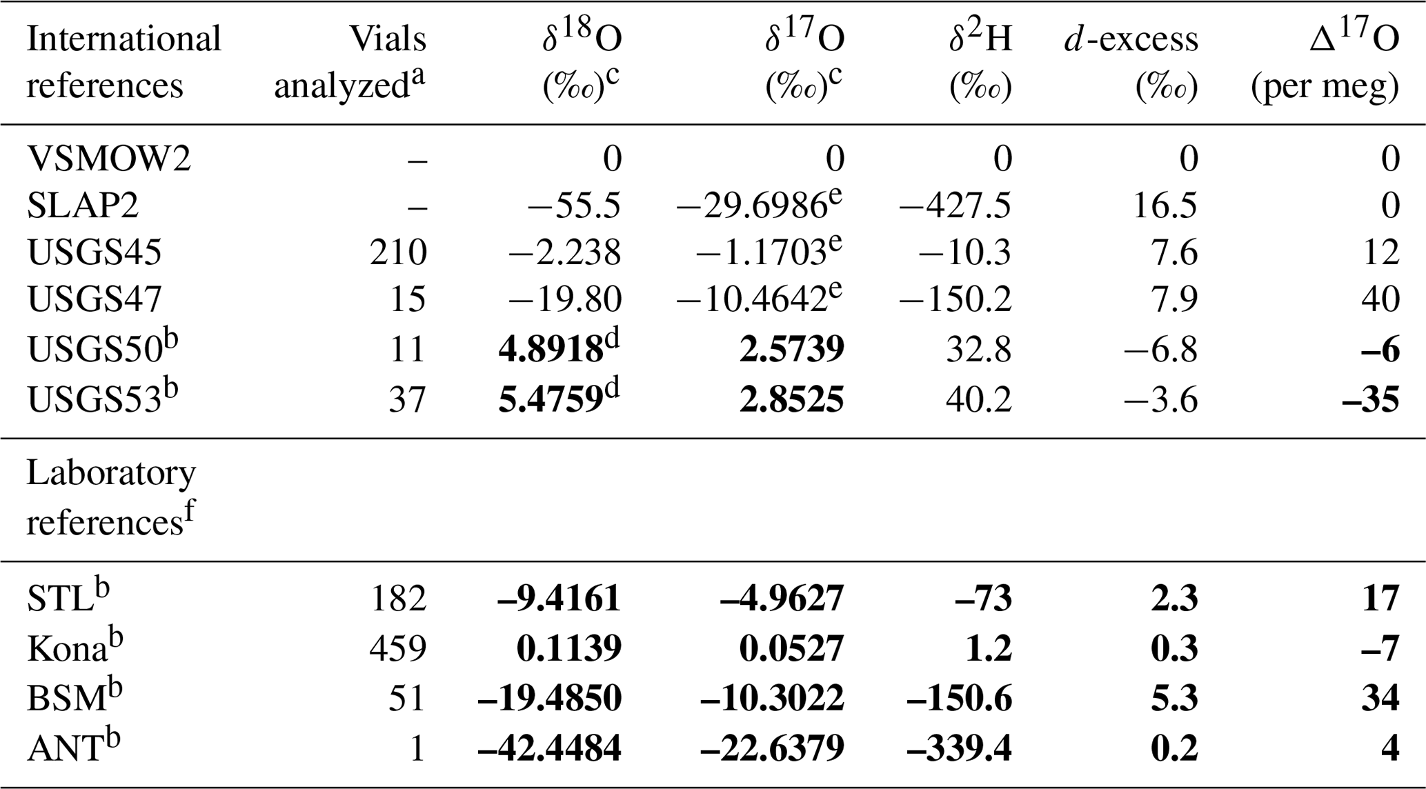
^a The number of discrete vials analyzed by this lab; it excludes any vials used for scale normalization. ^b International or laboratory reference waters whose ¹⁷O composition was previously unconstrained. ^c Up to 4 decimal places are reported to allow reproduction of Δ¹⁷O. For traditional interpretation of delta values, we use and recommend rounding to 2 decimal places. ^d We report our calibrated value rather than the recommended value for compatibility with our observed Δ¹⁷O. Additional, external analyses would be required to detect if the recommended value is subject to revision. ^e Values are derived from Berman et al. (2013). ^f STL: tap water from St. Louis, MO, USA; Kona: bottled drinking water from Kona Deep; BSM: tap water from Big Sky, MT, USA; ANT: ice core sample from Antarctica.

Table 2 Long-term performance of standard reference materials. Values for standard deviation (SD), root mean square error (RMSE), and mean signed difference (MSD) for all reference materials analyzed during the ∼ 2 year measurement period.

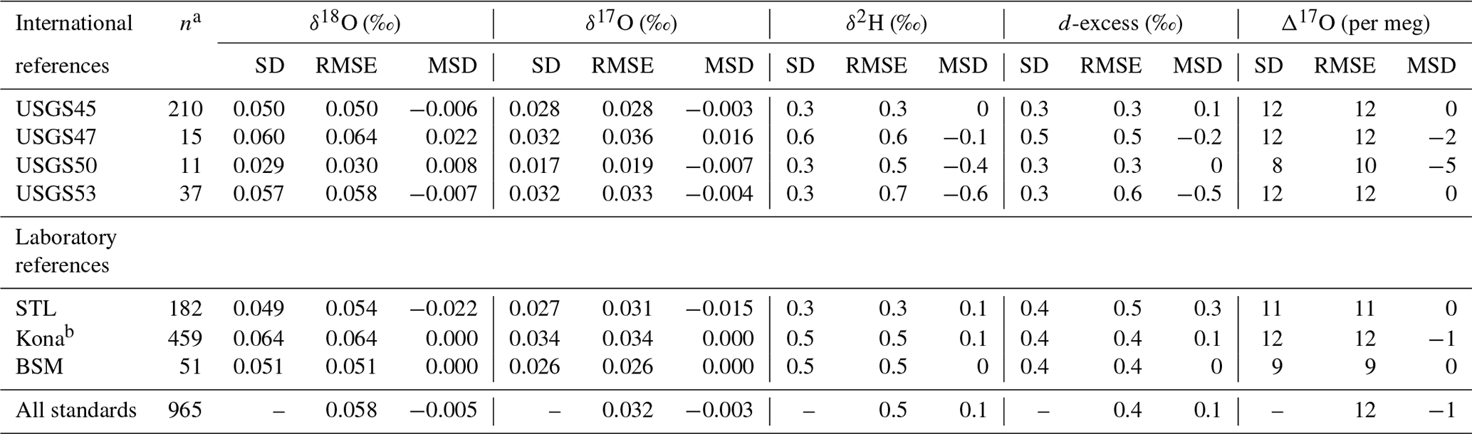
^a The number of discrete vials analyzed by this lab; it excludes any vials used for scale normalization. ^b Kona vials were used for drift correction and should not be strictly interpreted as control standards.

Primary reference waters (VSMOW2 and SLAP2) were used for scale normalization from January 2019 to June 2020 to establish acceptable performance of the instrument and to calibrate in-house laboratory reference waters and international reference waters previously unconstrained for ¹⁷O composition (Table 1). In-house laboratory reference waters were selected in order to (1) bracket the common range of δ¹⁸O and δ²H in natural waters across the globe and, in particular, to bracket low-latitude precipitation and surface water samples which are routinely analyzed in our lab and to (2) capture a large range of Δ¹⁷O values. Tap water from St. Louis, MO (STL), tap water from Big Sky, Montana (BSM), and bottled Kona drinking water from Hawaii (Kona) were stored in 30 L kegs following Tanweer et al. (2009). In addition, three 10 L polyethylene containers of melted Antarctic ice core (ANT) were stored in a cold room for occasional analysis of more ¹⁸O- and ²H-depleted samples. All secondary reference waters were measured independently for ¹⁷O composition at the University of Michigan via H₂O fluorination and analysis by dual-inlet isotope ratio mass spectrometry (Table S1 in the Supplement) using the same conditions as described by Li et al. (2015). Δ¹⁷O values produced by our Picarro (Table 2) for control standards have a precision (1 standard deviation) of 9–12 per meg (mean of 12). Our calibrated values are within the error of the independent measurements (Table S1).

Table 3 Typical sequence structure.

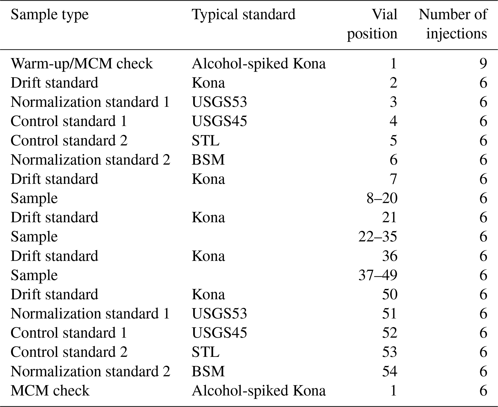
Sequences were structured to account for drift by bracketing unknowns with normalization and control standards with an additional drift standard injected between every ∼ 12 samples (Table 3). A warm-up vial was used consisting of our drift standard, which, for the final 6 months of the 18-month measurement period, was spiked with a small amount of ethanol (174 mg L⁻¹) and methanol (32 mg L⁻¹) to serve as a quality check on the combustion performance of the MCM. Each normalization/control standard set (vial positions 3–6 and 51–54 of Table 3) was ordered from more positive to more negative δ¹⁸O and δ²H values. Aside from the warm-up vial (nine injections), all vials used six injections of the extended long-pulse injection routine, resulting in a ∼ 14.4 min injection-to-injection duration and approximately 1.5 h analytical time per vial. Our typical sequence (Table 3) lasted ∼ 3.3 d and was designed to allow for some operator flexibility to ensure a regular schedule of two complete sequences (80 unknown vials) per week.

Unknown samples run during the study period were predominantly unfiltered rainwater, although ground-, tap-, and filtered river-water samples were run intermittently. Samples whose Δ¹⁷O was intended to be measured were typically analyzed with a minimum of three replicates as discrete, 200 µL aliquots spread across separate sequences. See Sect. 4.3 for the rationale. Samples were stored at 4 ^∘C in 4 mL glass vials with polyethylene PolyCone caps wrapped in Parafilm. During measurement, a sample was opened, and a 200 µL aliquot was transferred to a measurement vial. Storage vials were then recapped, fresh Parafilm applied, and stored again at 4 ^∘C.

2.2 Corrections for memory, instrument drift, and scale normalization

Sample-to-sample memory is a typical operating constraint of continuous flow instruments. The commonly suggested approach to reducing memory for Picarro water isotope analyzers is to perform at least six injections and discard all but the last three (Picarro Inc., 2015b). A second approach is to perform an empirical correction by estimating the size of the memory reservoir(s) and using this information to remove the influence of the previous vial (Van Geldern and Barth, 2012; Gröning, 2011). We implemented both approaches in our standard processing routine: correction of all injections following the “simple one-memory approach” of Gröning (2011) while also using only the last three injections of each vial for the calculation of isotope values. Memory coefficients, defined as the fraction of the current vial's contribution to the observed isotope value, were determined using a “memory term sequence” using 5 sets of 25 injection replicates alternating between an enriched sample (Kona, δ¹⁸O ≈ 0 ‰; Table 1) and a depleted sample (ANT, δ¹⁸O ≈ −42 ‰). The last eight injections of each were averaged to calculate the “memory-free” values and then used with simple isotope mass balance to calculate the fraction (i.e., memory coefficient) of the previous vial at each injection (Gröning, 2011). Memory coefficients were relatively stable over time. Memory coefficients were updated by running the memory term sequence every ∼ 3 months. We calculated memory coefficients only for primary isotope metrics (δ¹⁸O, δ¹⁷O, and δ²H). Any memory effect measured on the secondary metrics of d-excess and Δ¹⁷O are observed by comparing their calculations from corrected and uncorrected primary isotope data.

Instrument drift was accounted for by the repeated injection of discrete vials of Kona (Table 1) spread throughout the sequence (Table 3). The Kona standard was selected because most unknowns analyzed in this period were relatively enriched, tropical rainfall samples. Given the length of our sequences (∼ 3.3 d), the maximum daily drift according to specifications of 0.2 ‰ (for oxygen) and 0.8 ‰ (for hydrogen) can well exceed measurement precision of 0.025 ‰ and 0.1 ‰, respectively (Picarro Inc., 2017). Our drift correction was based on a linear regression of the drift standard delta values versus injection position, the latter of which is a proxy for time. To apply the drift correction, the slope of the drift regression was multiplied by an injection's position, and the product then subtracted from the injection's observed delta value. This was calculated and applied independently for δ¹⁸O, δ¹⁷O, and δ²H. Our L2140-i did not always exhibit linear drift, and so the choice to perform the drift correction was made on a per-sequence basis.

Normalization to the VSMOW–SLAP scale was achieved by linear regression of the normalization standards. As the Picarro factory calibration is relatively stable over time, raw δ¹⁸O values are typically within ∼ 1 ‰ of the corrected values; however these small variations result in the uncorrected Δ¹⁷O being hundreds of per meg away from calibrated values (Fig. S12). Uncorrected δ²H, however, has tended to drift directionally over time by ∼ 5 ‰ (Fig. S12). Typically, USGS53 and BSM (Table 1) were used as normalization standards. Both the starting and ending sets of standards were used for scale normalization, yielding some averaging of instrument noise that may otherwise impact “true” two-point linear normalization (Paul et al., 2007).

2.3 Processing

Post-run processing to apply the various corrections (Sect. 2.2) was performed using an R script (supplemental file S1), following the approach of Schauer et al. (2016). The L2140-i produces four levels of data reduction: spectral, private, user, and coordinator data (Schauer et al., 2016). Spectral data are recorded as hierarchical data format (HDF) files and contain the absorbance values from each ring-down analysis with approximately 400–500 discrete measurements per second. Private data, referred to in this paper as “high-resolution data”, are also in the HDF file format and are a reduction of the spectral data format at approximately 1 Hz containing integrated absorbances for each isotopologue, as well as a wide array of other instrument variables. User data are a subset of high-resolution data (i.e., private data) variables exported at the same temporal resolution (1 Hz) as a tab-delimited file. Coordinator data are the default user-facing data product and integrate (i.e., averages) the data for each injection as a single line containing the mean and standard deviation of isotope values, as well as a very limited subset of diagnostic results. See Schauer et al. (2016) for greater detail about the L2140-i's data types. Our post-processing approach used the high-resolution data product. After the user collected the appropriate high-resolution data for a sequence based on date and time, our processing script read the HDF files, used a set of criteria to find each injection (or pulse) based on H₂O levels, and assigned them to injections in a sequence based on user input and our sequence template (supplemental file S1). Each injection contained ∼ 430 measurements based on the time it took to generate one line of high-resolution data (∼ 1 Hz) and the duration of usable data (∼ 8 min) during each injection cycle of the long-pulse mode. Concentration ratios (R) of heavy-to-light isotopologues corresponding to each isotope system (Table S2) were used to calculate delta values expressed in per mil notation:

$$\begin{array}{}\text{(1)}& \mathit{\delta }=\left(R_{\mathrm{sample}}/{\mathrm{R}}_{\mathrm{standard}}-\mathrm{1}\right)\times \mathrm{1000},\end{array}$$

where R_sample corresponds to the observed signal, and R_standard corresponds to the observed R of an injection of VSMOW2 performed shortly after the instrument installation. The δ values correspond roughly, but not exactly, to the default, uncalibrated δ values shown by the Picarro data viewer and coordinator software during analysis. Schauer et al. (2016) noted that δ²H experienced increased memory during the long-pulse mode and recommended using only the first ∼ 200 s of δ²H data when integrating (via the arithmetic mean) each pulse, while the oxygen delta values should use the full pulse. Our initial testing found that 180 s was optimal for δ²H, and our script used this value, although this may be an instrument-specific variable. Injections were then memory corrected, summarized to the vial level using the last three injections of each vial, assessed for drift correction, and then scale normalized. The derived values of deuterium excess (d) and Δ¹⁷O were calculated from the fully corrected isotope values. Deuterium excess was defined as

$$\begin{array}{}\text{(2)}& d\text{-excess}={\mathit{\delta }}^{\mathrm{2}}\mathrm{H}-\mathrm{8}\left({\mathit{\delta }}^{\mathrm{18}}\mathrm{O}\right),\end{array}$$

while Δ¹⁷O was defined as

$$\begin{array}{}\text{(3)}& \begin{array}{rl}{\mathrm{\Delta }}^{\mathrm{17}}\mathrm{O}& =\left(\ln \left({\mathit{\delta }}^{\mathrm{17}}\mathrm{O}/\mathrm{1000}+\mathrm{1}\right)\right.\\ & \left.-\mathrm{0.528}\times \ln \left({\mathit{\delta }}^{\mathrm{18}}\mathrm{O}/\mathrm{1000}+\mathrm{1}\right)\right)\times {\mathrm{10}}^{\mathrm{6}}\end{array}\end{array}$$

using a slope of 0.528 (Luz and Barkan, 2010) and expressed in per meg (10⁶).

Our processing script produces an Excel file containing sheets that report various layers of data reduction: calibrated results of samples, summary statistics and results of quality control standards, injection-level and vial-level results corrected only for memory, and some additional diagnostic results and metadata. Sample results are output both rounded (for general reporting) and unrounded for easy recalculation of Δ¹⁷O values. Summary statistics for control standards include observed arithmetic mean, observed standard deviation, the root mean square error, and mean signed difference. Root mean square error (RMSE) was calculated as

$$\begin{array}{}\text{(4)}& \mathrm{RMSE}=\sqrt{{\displaystyle \frac{\sum _{i=\mathrm{1}}^n{\left(x_i-{\widehat{x}}_i\right)}^{\mathrm{2}}}{n-\mathrm{1}}}},\end{array}$$

where x_i is the final, calibrated value of a standard, and ${\widehat{x}}_i$ is the current accepted value for that standard. The mean signed difference was calculated as

$$\begin{array}{}\text{(5)}& \mathrm{MSD}={\displaystyle \frac{\sum _{i=\mathrm{1}}^n\left(x_i-{\widehat{x}}_i\right)}{n}}\end{array}$$

following the same notation as RMSE. RMSE is used as the primary measure of precision and accuracy, while MSD provides an estimate of bias from the accepted value. We also provide an R script (supplemental file S2) that performs post-processing operations on Picarro's coordinator data output. The coordinator data script is not able to utilize the shortened integration time of δ²H measurements but does perform memory, drift, and scale-normalization corrections.

2.4 Statistical methods

All data analysis and plotting were performed within R (R Core Team, 2017) using the tidyverse package set (Wickham et al., 2019). Picarro's HDF files were read using the rhdf5 package (Fischer et al., 2020). All statistical hypothesis testing was performed by application of a balanced bootstrap approach using an appropriate sampling statistic (e.g., arithmetic mean, ordinary least-squares slope), and the statistic's 95 % confidence interval was tested for overlap with zero to test for significance, which is equivalent to a p value cutoff of 0.05 for null hypothesis testing (Davison et al., 1986). Unless otherwise noted, errors on summary statistics reported in Sect. 3 (given in brackets) are the 95 % confidence interval.

3 Results

3.1 Memory corrections

Memory coefficients generated by memory term sequences as described in Sect. 2.2 show little variation over the measurement period (Fig. 1). δ¹⁸O and δ¹⁷O have nearly identical memory effects and averaged 98.8 % (98.7 %–98.9 %) of current vial contribution to the current pulse by the fourth consecutive injection from a vial, which falls slightly short of the stated efficiency of 99 % by Picarro. This slight deviation may be due to the increased flow path introduced by the MCM device or due to our longer pulse duration than the high-precision mode. As expected, δ²H experiences greater memory and achieved 98.4 % (98.3 %–98.4 %) current vial contribution by the fourth consecutive injection, which slightly exceeds Picarro's stated performance of 98 %. The shortened δ²H data usage note in Sect. 2.3 may explain the improved performance. Our currently limited dataset (n = 2 sequences) for the high-precision mode indicates the performance for δ²H matches the 98 % specification (fourth injection mean of 98.0 %). Correction for memory improves the RMSE of control standards in the case of all metrics except Δ¹⁷O where no difference was observed (Fig. S1). The magnitude of improvement was ∼ 0.05 ‰ for δ¹⁸O and δ¹⁷O and ∼ 0.5 ‰ for δ²H.

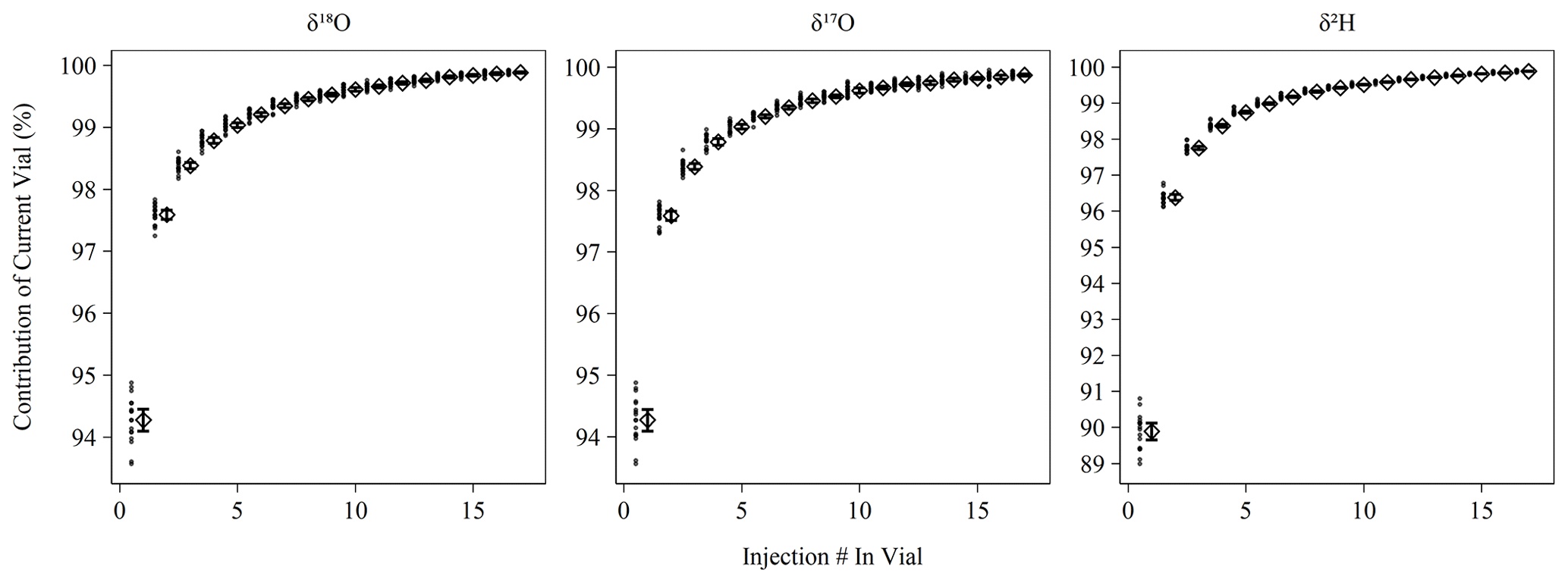
Figure 1 Percent contribution of the current vial's injection to the observed isotopic measurement based on memory term sequences (Sect. 2.2). Long-term mean and 95 % bootstrapped confidence interval shown as diamonds and error bars, respectively, with contribution estimates from individual memory coefficient runs shown as filled circles. Note that δ¹⁸O and δ¹⁷O have different y axis ranges than δ²H.

3.2 Drift corrections

Instrument drift on the L2140-i is rated at a maximum of 0.2 ‰ d⁻¹ for oxygen measurements and 0.8 ‰ d⁻¹ for hydrogen measurements (Picarro Inc., 2017). Our assessment of drift using the Kona standard as outlined in Sect. 2.2 indicated significantly less drift than the maximum specification during the 2-year measurement period (Fig. 2). Hydrogen measurements were almost always drift corrected, whereas oxygen measurements showed more variability and more often had sequences whose drift slope approached zero. However, for both oxygen and hydrogen measurements during the measurement period, the average drift slope was significantly different from zero as shown in the confidence intervals of Fig. 2. When combined with the sequence length of ∼ 3.3 d, the magnitude of the daily drift rates (Fig. 2) exceeds typical instrument error (Table 2) by ∼ 0.06 ‰ and ∼ 0.4 ‰ for oxygen and hydrogen measurements, respectively.

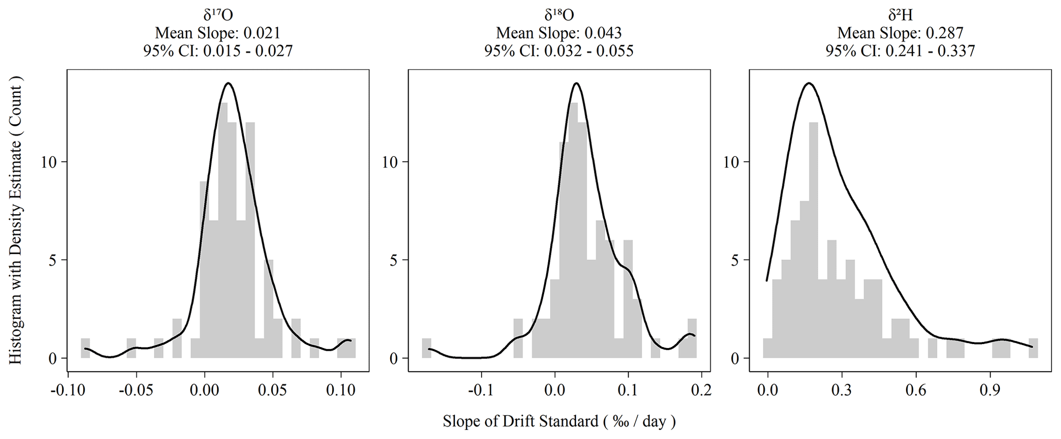
Figure 2 Histograms of ordinary least-squares regression slopes of drift standard isotope values versus elapsed sequence time. Summary statistics are presented above each plot. The 95 % confidence intervals are the 2.5 and 97.5 percentiles of the bootstrapped distribution of mean slopes.

In addition to our standard drift-correction procedure, we tested several alternative approaches to drift correction. This was necessary to account for the multiple possible causes of instrument drift, which are not well understood but which would have different consequences for sequence structure and other practicalities of routine sample analysis. Further, the long-term drift slopes in Fig. 2 are all significantly different from zero, which indicates that the L2140-i – at least our specific unit – exhibits positive directional drift (i.e., more positive isotope values over time). On the time scale of individual sequences, drift is observed to vary beyond the long-term mean with oxygen measurements sometimes even exhibiting negative drift slopes (Fig. 2). The variability of short-term drift – i.e., the observed drift at the sequence level – may be due to extrinsic, time-varying factors (e.g., environmental conditions), or it may be due to the fact that the magnitude of the drift is comparable to short-term instrumental precision. If the former is true, then a series of drift standards with each sequence is necessary to capture the impact of these time-varying factors, as in our standard operating procedure. If the latter is true, then simply a large sample size of sequences is necessary to estimate the true drift terms (e.g., Fig. 2), and then these terms can be applied to each sequence without accounting for sequence-level drift standards. Finally, alternative approaches were tested to account for drift that is non-linear and/or inconsistent over time.

Table 4 Accuracy metrics for all control and drift vials of known isotope composition for various drift-correction approaches. Values for root mean square error (RMSE) and mean signed difference (MSD; in parentheses) for all vials analyzed during the ∼ 2 year measurement period.

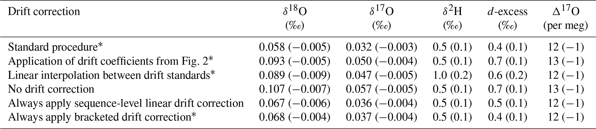
^∗ See Sect. 2.2.

To test these alternatives, we used the long-term coefficients from Fig. 2 to correct all the sequences during our measurement period and calculated RMSE and MSD and found worsened performance compared to our standard drift-correction procedure for most isotope measurements (Table 4). We also reprocessed sequences by drift correcting using linear interpolation between individual drift standards, which would better account for non-linear drift. Linear interpolation between individual drift standards also produced worsened performance for most isotope measurements (Table 4). As an alternative to our standard procedure of applying a drift correction only when the drift standards vary directionally, we also reprocessed sequences completely leaving out the drift correction, by always applying the drift correction and by always applying the drift correction calculated from only the first and last bracketing drift standards (Table 4). Always applying sequence-level linear drift correction using either all the drift standards or only the first and last bracketing drift standards provides results very close to our standard procedure (Table 4), although this should be expected as our standard procedure typically applies the sequence-level linear drift correction. Long-term performance of Δ¹⁷O was insensitive to the method of drift correction.

3.3 Contamination by organic compounds

Organic contamination during the last 6 months of the measurement period was monitored as described in Sect. 2.1 with the use of a sample of our Kona standard spiked with amounts of ethanol and methanol following Picarro's recommendations for assessing MCM cartridge health for δ¹⁸O and δ²H in the user manual (Picarro Inc., 2015a). The MCM manual suggests using a “simulated plant water” solution ranging from ∼ 1.3 % (v:v) alcohols to ∼ 0.26 % (v:v) alcohols, equivalent to 10 648 and 2130 mg L⁻¹, respectively. In these cases, Δ¹⁷O is elevated by well over 1000 per meg. The concentration employed in our MCM quality assurance standard as described in Sect. 2.1 is equivalent to a 50-fold dilution (∼ 213 mg L⁻¹) of the original 1.3 % solution and results in a Δ¹⁷O elevation of ∼ 100 per meg without the use of the MCM (or when the MCM cartridge has failed). Elevation of Δ¹⁷O due to spiked alcohols is detectable from the unspiked standard in as little as 42 mg L⁻¹ or ∼ 250-fold diluted from the original 1.3 % alcohol solution. The threshold for detectable alteration of the measurement is similar for other isotope measurements (Fig. 3). An MCM cartridge was considered spent when the MCM quality assurance standard exceeded +100 per meg relative to the pure Kona standard, which was always observed to occur as a single step rather than a partial failure over a series of injections. However, as the quality assurance standard only bracketed sequences, we do not know the exact failure mode of the cartridges except that it occurs over the duration of a single sequence. During the 6 months of routinely operating with the MCM on, we exchanged five cartridges. Each cartridge lasted between 5 and 75 d with an average lifetime of 31 d. Therefore, the extreme sensitivity of Δ¹⁷O to organic contamination makes the effective cartridge lifetime much shorter than the expected 4 months of operation when analyzing only δ¹⁸O and δ²H (Picarro Inc., 2015a).

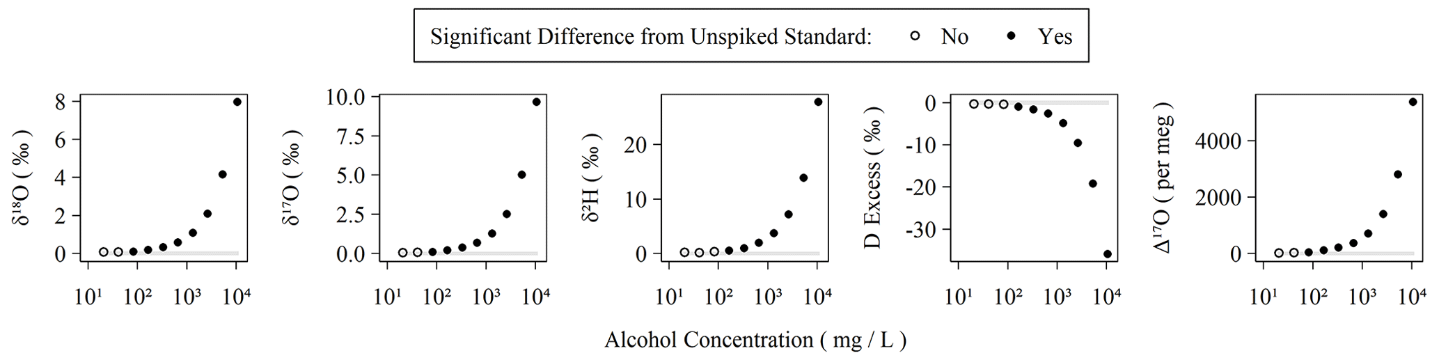
Figure 3 Observed isotopic measurements with increasing amounts of alcohols spiked into our Kona lab standard. The highest concentration here corresponds to 1.1 % (v:v) ethanol and 0.2 % (v:v) methanol and was serially diluted in 50 % steps to generate the remaining points. Each concentration was measured using two replicate vials with six injections each. The average and standard deviation of the last three injections of each vial were compared to triplicate vials of the Kona standard using a Monte Carlo approach, which simulated normal distributions from the observed averages and standard deviations, and were then subjected to a balanced bootstrap unpaired test of differences in the mean values and then evaluated at the 95 % confidence interval level.

We tested and developed several techniques for flagging samples with suspected organic contamination. First, in some cases, visual inspection of the data is sufficient to flag samples of possible concern because the measurements lie well outside the observed natural range of Δ¹⁷O in meteoric waters (approximately −50 to +60 per meg although values are most commonly positive; Aron et al., 2021). Second, the L2140-i produces diagnostic values based on spectral characteristics to help the user determine if organic contamination has occurred. However, Picarro's ChemCorrect software is unable to correct for interference and moreover does not operate on ¹⁷O mode data (Picarro Inc., 2015b). Our standard procedure used these suggested values to flag samples that may be “contaminated”. Third, we developed a potentially more sensitive metric for detecting contaminated samples that makes use of two spectral peaks for the ¹⁸O-containing water isotopologue (referred to hereafter as the “¹⁸O​​​​​​​ laser flag”). The ¹⁸O laser flag was calculated as the standard deviation of the instrument's two δ¹⁸O values corresponding to spectral peak ratios (see Table S2) of peak 11 to peak 2 (used for ¹⁷O mode δ¹⁸O measurement) and peak 1 to peak 2 (used for normal mode δ¹⁸O measurement but still operated in ¹⁷O mode). The two ¹⁸O-containing spectral peaks are measured independently by two different lasers, and their peak absorbances are separated by ∼ 7 cm⁻¹ (Steig et al., 2014). The response factors of each ¹⁸O-containing peak to concentration were different by about a factor of 1.7 and required some form of normalization for comparison. As we were already calculating their apparent δ¹⁸O during processing, and this calculation implicitly accounts for their different response factors by use of a reference standard, we chose to use the two δ¹⁸O results and their standard deviation in the familiar per mil notation to assess the ¹⁸O laser flag. During sequence processing, we calculate the maximum ¹⁸O laser flag value among non-spiked standards and add 0.05 ‰ (an arbitrary factor equivalent to ∼ 2–3 standard deviations of internal precision). Samples whose ¹⁸O laser flag exceeds this threshold were flagged as potentially contaminated.

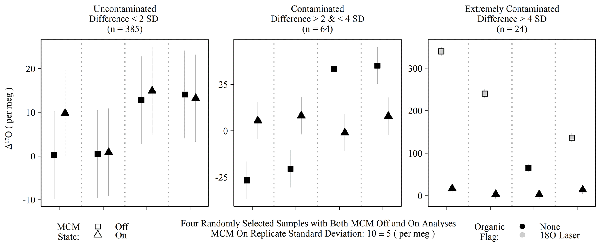
Figure 4 Randomly selected subset of calibrated Δ¹⁷O of samples run with the MCM off and on categorized into three groups based on the differences between the MCM off and on analyses. Differences exceeding 2 standard deviations of instrumental precision are assumed to derive from organic contamination. Only “extremely contaminated” samples are typically identified by spectral flags as having organic interference (grey-filled points).

The MCM is a peripheral device recommended by Picarro when users intend to analyze samples with substantial organic interference, such as plant waters. Initially, we operated the instrument with the MCM in warm mode (hereafter MCM off) for two reasons: first, we were measuring pure rainwater and tap water samples and therefore did not expect significant organic contamination, and second, we expected any minor contamination would be detected via Picarro's spectral contamination flags. This initial batch of MCM off samples (n = 473) contained 16 calibrated Δ¹⁷O values that greatly exceeded the expected natural range (as high as 628 per meg). Those unusual samples nearly always (15 out of 16) exceeded the threshold of our ¹⁸O laser flag when the Δ¹⁷O exceed 100 per meg but were only flagged by Picarro's suggested metrics in extreme cases (> 500 per meg). Due to this variable flagging, we reran replicates from this batch with the MCM on and found that Δ¹⁷O for obviously contaminated samples (i.e., both spectral flags and extreme Δ¹⁷O) was then shifted to within the expected natural range for meteoric waters: the full range of MCM on Δ¹⁷O values was −61 to 58 per meg. False negatives – MCM off samples with no contamination flags but excessively different Δ¹⁷O values from their MCM on replicates – were determined by comparing Δ¹⁷O differences between MCM modes and used either a 2 or 4 standard deviation threshold of 20 or 40 per meg, respectively, based on instrumental precision. Differences between 20 and 40 per meg were categorized as contaminated, whereas differences > 40 per meg were categorized as extremely contaminated. Only 15 of the 24 extremely contaminated samples were spectrally flagged, and none of the 64 samples from the contaminated group of Fig. 4 triggered any type of spectral flags. All extremely contaminated samples had elevated Δ¹⁷O, whereas the contaminated group was roughly split between positive and negative biases. While some of the contaminate group (14 % of MCM off samples) may simply be uncontaminated outliers, only 4 % of individual MCM on replicates were greater than 20 per meg away from their replicate means, which is consistent with 2 standard deviations, accounting for ∼ 95 % of a normal distribution. All of the 473 samples compared in this section were rainwater samples from which we would have no a priori reason to expect organic contamination.

3.4 Long- and short-term precision and accuracy

The long-term performance for standard reference materials on the L2140-i within the measurement period is summarized in Table 2. The long-term precision of standards (i.e., the standard deviation of final, calibrated values) was essentially identical to our primary measure of accuracy (RMSE) due to the relatively small bias in accuracy as measured by MSD. Long-term summary statistics can mask some variability in sequence-to-sequence performance, so we also summarized standards at the sequence level (Fig. 5). Sequence-level mean values (Fig. 5, Table S3) for RMSE and MSD are essentially identical to long-term performance (Table 2). However, short-term bias in accuracy can be a much larger factor than long-term bias, with the standard deviation of MSD at the sequence-level about 50 % the size of RMSE (Fig. 5, Table S3). This effect is not typically problematic for primary isotope measurements due to the already small error, but for Δ¹⁷O the standard deviation of sequence-level MSD (Fig. 5, Table S3) is 6 per meg, which can indicate systematic error at the sequence level. The USGS45 standard was included as a control in all sequences, as its Δ¹⁷O has some consensus, and its calibrated values all converged on the current accepted values (Table 2) with consistent performance through time (Fig. S4).

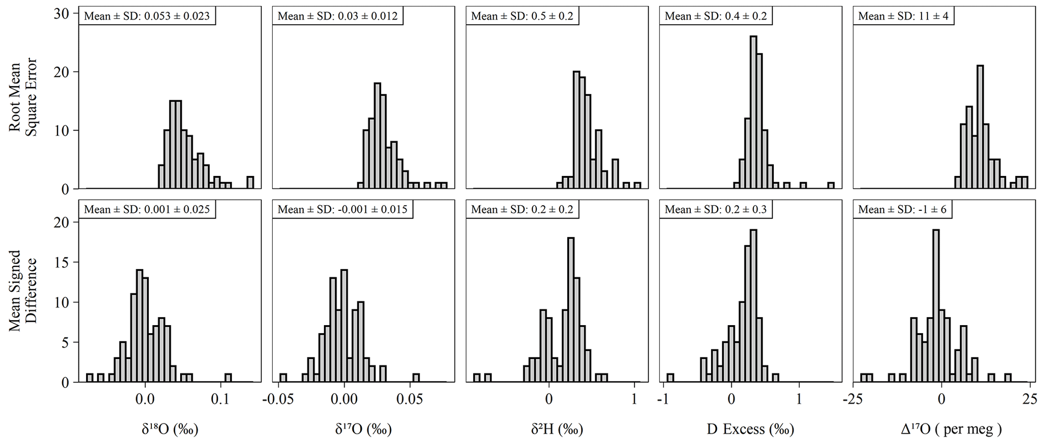
Figure 5 Histograms of accuracy metrics (see Sect. 2.3 for formulas) for all sequences (n = 85) run during the study. Note that RMSE cannot be less than zero. Under ideal conditions, the mean MSD is equal to zero. Means and standard deviations (SD) shown above each histogram for each pairing of isotope measurement and accuracy metric.

The duration of the measurement period of replicate samples had a small but weak influence on replicate precision. For measurement of Δ¹⁷O in unknown samples, we utilized discrete vials measured across multiple sequences, an approach that provides a measure of medium-term precision (i.e., reproducibility across a limited set of sequences) and produces optimal mean errors (see Sect. 4.3 and 4.5). The average standard deviations of unknown samples for each measurement type (Fig. S3) are equal to or exceed the long-term performance of standards (Table 2). The use of discrete sequences for unknowns resulted in a mean measurement period of 7 (range: 0–21) months as defined by the first and the last time an unknown was measured. There were weak but significant relationships of unknown replicate precision versus the measurement period for all isotope metrics (Fig. S5), and all relationships became insignificant when the data were more equally weighted using 2-week binned average standard deviations (Fig. S6). Our sample storage strategy of 4 mL vials using polyethylene PolyCone caps wrapped with Parafilm stored in a refrigerator at 4 ^∘C is apparently effective for at least the storage duration of the study period.

The standard deviation of the last three injections of a vial was used as a measure of short-term precision. We used this metric to assess overall short-term precision across the entire measurement period (Fig. S7, n = 4112 discrete vials) and to evaluate the impact of the instrument's two measurement modes and pulse length on short-term precision. The varying operation modes (normal mode versus ¹⁷O mode) and pulse length routines (high precision versus long pulse) were compared by running replicate sequences (n = 48 vials each) in each of the modalities and assessed using paired differences. In ¹⁷O mode, the results of this experimental comparison (Fig. S8) indicated that the long-pulse routine improves precision for δ¹⁷O, δ¹⁸O, and Δ¹⁷O relative to the high-precision routine. Pulse length did not produce significant improvements in the short-term precision of δ¹⁸O when operated in normal mode (i.e., ¹⁷O disabled; Fig. S8). When comparing ¹⁷O mode vs. normal mode (Fig. s9), operating the instrument in normal mode (i.e., ¹⁷O disabled) improved the precision of δ¹⁸O by an average of 0.010 ‰ (0.007 ‰–0.012 ‰), whereas ¹⁷O mode improved the precision of δ²H by an average of 0.15 ‰ (0.12 ‰–0.17 ‰) with no differences between modes for d-excess. The short-term precision during this limited experiment was similar to the entire measurement period (Fig. S7).

Finally, we assessed the influence of data source (Picarro's high-resolution data vs. coordinator data) on precision. Our standard data processing approach used Picarro's high-resolution output via our R processing script (supplemental file S1). An alternative processing approach (supplemental file S2) uses Picarro's default user-accessible coordinator data output via a modified R script written to ingest the coordinator output's simple comma-separated values (CSV) files. In principle, the only differences between these methods were that the high-resolution approach used our own pulse-detection parameters (versus those hard coded into Picarro to generate coordinator data) and that our high-resolution data script uses only the first ∼ 180 s of each pulse for determining δ²H versus the entire pulse for coordinator data (Schauer et al., 2016). All corrections (memory, drift, and scale normalization) were calculated in the same way. To compare the two approaches, we processed ∼ 6 months of sequences from the first half of 2020 (16 standard sequences with 3 memory term sequences) using both R scripts. Significant differences in short-term precision between the two approaches were found for δ¹⁷O, δ¹⁸O, and Δ¹⁷O, with the high-resolution approach having 3.9 %, 2.4 %, and 6.5 %, respectively, smaller standard deviations than coordinator data (Fig. S10). These values were calculated using the mean absolute differences between the processing approaches and dividing it by the precision of the high-resolution results. Despite differences in short-term precision, standards with known isotopic composition had statistically indistinguishable RMSE values for all measurements except δ²H (Fig. S11).

4 Discussion and recommendations for operational procedures

4.1 Corrections

In our standard protocol, we apply three corrections: memory, drift, and scale normalization. Of these, the only correction commonly understood to be necessary is that of scale normalization – required to place the uncalibrated data on the internationally accepted VSMOW–SLAP scale (Paul et al., 2007). Corrections for memory and drift are commonly applied by users of laser-based isotope instruments (Chesson et al., 2010; Van Geldern and Barth, 2012), although various approaches are possible (Berman et al., 2013), and some analytical conditions can be maintained to avoid these corrections (Schauer et al., 2016). However, the necessity of corrections is determined by the level of precision and/or accuracy needed by the end user and their research question. The addition of standards to measure and account for these corrections consumes both analyst and analyzer time, and thus the choice to apply them must balance the investment of time against the requirements of instrument performance. While the application of post-analysis corrections to data is necessary, such corrections should be minimized to prevent “overcorrection”, i.e., introduction of bias and/or artifacts (e.g., overfitting of low signal-to-noise relationships, incorrectly modeling the function to be accounted for). Here, we discuss the impact of each of these corrections and their relative importance for different users and applications.

Memory correction was determined by an empirical isotope balance mixing model as described in Sect. 2.2 following Van Geldern and Barth (2012). Memory coefficients determined this way showed little variation over the 2-year measurement period (Fig. 1) and significantly improved all isotope measurements except Δ¹⁷O (Fig. S1). Other users have chosen different approaches to handling instrument memory. Efforts to avoid memory correction include increasing the number of discrete measurements in a vial or the ordering of measurements to ensure adjacent measurements are isotopically similar (Schauer et al., 2016), which in both cases minimizes the impact of sample-to-sample memory. The former effect can be seen in Fig. 1 where memory is increasingly diminished with consecutive measurements, with the primary trade-off being an increase in analyzer time spent on a single vial. The latter effect of “isotopic ordering” is only possible if approximate isotopic values are known a priori, which is only possible in certain situations (e.g., directional measurement of ice cores) or with preliminary isotopic measurement. In our laboratory, our measurements typically target meteoric waters that vary widely on an event-to-event basis and would require preliminary measurement to order. Even then, this approach would still be problematic because ensuring small isotopic differences between all adjacent unknowns may not be possible for any given batch of samples. We therefore find the method of calculating and applying memory coefficients to be practical as well as effective in minimizing sample-to-sample memory for routine analysis of unknown meteoric waters with a wide range of variability. Calculation of memory coefficients is done through a memory term sequence as described in Sect. 2.2 and measured on a ∼ 3-month interval, while application of coefficients is done during post-processing. Aside from the requirement of determining the memory coefficients, this does not add significant analysis time as this correction does not require positions in a standard sequence to be applied.

Drift correction used a sequence-level linear regression slope of drift standards as described in Sect. 2.2 and followed standard practice in continuous flow applications. Correction for drift requires that the user includes a series of replicates of a standard to measure the observed drift during a sequence. Our standard sequence structure uses five drift replicates (Kona; Table 3) and, thus, consumes approximately ∼ 9 % of a sequence's run time. The benefits of drift correction are predominantly in improving the accuracy of δ¹⁸O, δ¹⁷O, and d-excess with RMSE approximately halved compared to not drift correcting (Table 4). However, there is no consistent effect observed for either δ²H or Δ¹⁷O. The lack of consistent improvement for δ²H, which itself has the largest daily drift values (Fig. 2), is surprising and suggests that the larger errors inherent with δ²H measurement may outweigh the effect of drift. Considering the range of isotopic variability in natural samples, the improvement to RMSE is substantial for δ¹⁸O (0.107 ‰ uncorrected vs. 0.058 ‰ corrected; Table 4) and perhaps less meaningful (or nonexistent) for the other quantities. These results suggest that omitting drift correction may be an appropriate decision if the end user is accepting of higher error for δ¹⁸O, δ¹⁷O, and d-excess. The opportunity cost of drift correction is not negligible: if our typical sequence structure (Table 3) was adjusted to exchange the drift standards for unknown samples, then our overall throughput of unknowns would be increased by 12.5 %. An appropriate compromise might be including drift standards only in the beginning and end of each sequence (bracketed drift correction in Table 4), which performs only marginally worse than our standard procedure, while also still increasing sample throughput compared to our typical sequence by 7.5 %. The primary drawback of this compromise is that the operator has little visualization of the drift effect during the sequence and would be obligated to simply always apply the slope calculated from the two drift standards.

Scale normalization is mandatory to ensure compatibility of interlaboratory measurements. Additionally, measurements made within a laboratory but separated in time benefit from increased comparability via scale normalization. However, we note that there may be some unique circumstances or applications for which scale normalization would not be strictly necessary. For example, the device could be used for measuring artificially enriched isotopic tracer samples whose differences are expected to exceed long-term variation. In our lab, the long-term instrumental drift on the Picarro L2140-i is surprisingly small for δ¹⁸O and δ¹⁷O (∼ 2 ‰ and ∼ 1.5 ‰ ranges, respectively) with directional drift of ∼ 6 ‰ for δ²H (Fig. S12). Due to the sensitivity of Δ¹⁷O, its long-term variation is extreme with a range of ∼ 600 per meg. Therefore, measurement of pulses of highly enriched isotope samples could yield largely satisfactory results without scale normalization, although such results would not necessarily be on the VSMOW–SLAP scale except in the loosest sense.

4.2 Error structure of replicate analyses and implications for Δ¹⁷O

The relative magnitude of the natural range of meteoric Δ¹⁷O (∼ 110 per meg, Aron et al., 2021) to the short-term precision of the measurement (∼ 11 per meg) – a ratio of 10 to 1 – is distinct from the other data streams produced by the L2140-i, which have range-to-precision ratios at least an order of magnitude greater than Δ¹⁷O. This may be an exaggeration when considering samples from a specific locality where the range of observed values is much smaller than the global range. However, for example, δ¹⁸O would need a natural observed range of only 0.164 ‰ to match the 10 to 1 ratio of Δ¹⁷O.

In other analytical settings, such as with isotope ratio mass spectrometry, a common approach to overcoming issues of precision is to perform repeat measurements and report their final average (Berman et al., 2013). If each measurement is a sample from a distribution with shape dictated by the performance of the instrument, then the average of repeated measurements will approach the average of the distribution, which itself approximates the true value if bias is sufficiently small (Miller and Miller, 1988). In the case of the L2140-i (and likely other CRDS instruments), the sequence-level bias (MSD) has variability equal to approximately 50 % of the long-term RMSE (Fig. 5). As such, distributing replicate measurements within a single sequence would not be adequate for approaching the true value. Therefore, we choose to distribute our replicate measurements across distinct (i.e., independently calibrated) sequences in an approach similar to many IRMS and some IRIS applications (Uechi and Uemura, 2019). As the average bias of sequences is close to zero (Table 2, Fig. 5), this approach should effectively minimize the impact of bias. While our approach takes more effort than preparing replicate vials for measurement in a single sequence, for our scientific purposes the impact on error minimization is well worth the effort, and we can be much more confident that the mean of our replicates minimizes sequence-level accuracy bias.

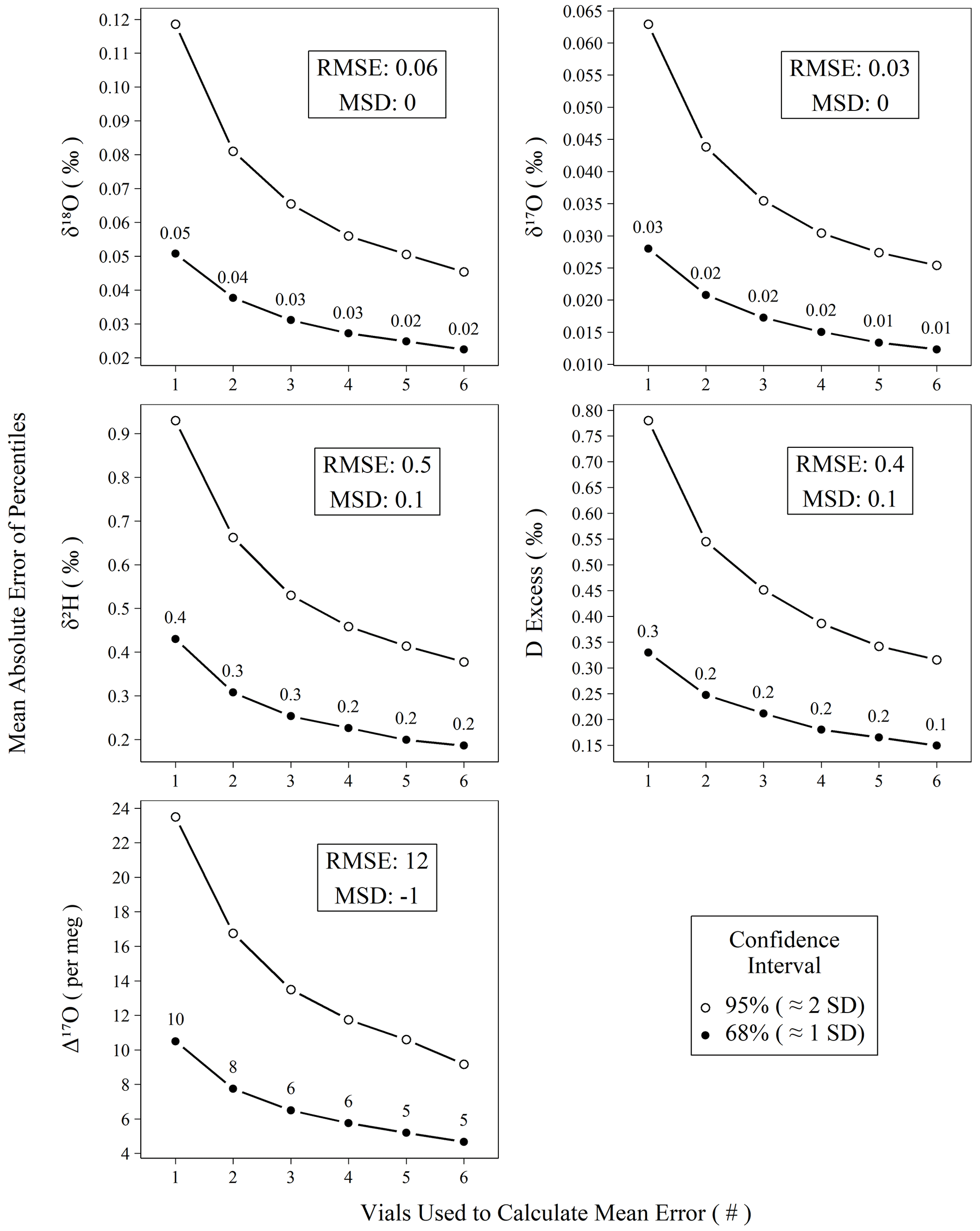
Figure 6 Mean absolute error of calibrated standards for isotope measurements versus the number of vials averaged prior to mean error calculation. All measurements of control and drift standards (n = 896) were subtracted from their accepted values, resampled (n = 100 000) without replacement into replicates of varying (1–6) size, and summarized as means to create probability distributions of mean errors. Confidence intervals (68 % and 95 %) were calculated for the probability distributions, and the mean absolute values of their percentiles are plotted against their replicate size. The two intervals chosen, 68 % and 95 %, roughly correspond to 1 and 2 standard deviations, respectively.

Figure 6 demonstrates the effect of replicate measurements using all control and drift standards analyzed during the study period. The decrease in error (i.e., width of the confidence interval) with an increasing number of averaged vials follows the trend in the standard error of the mean. Using only the n = 1 data from Fig. 6, we can predict the observed error structure of increasing replicates according to the standard error the mean (Fig. S13) with all r² > 0.99, which strongly indicates our error structure is normal. Figure 6 can be used to estimate the number of replicates needed to achieve a certain error threshold for unknown samples. Other users seeking to reproduce our performance should observe a very similar error reduction gradient as shown in Fig. 6, assuming comparable long-term instrumental performance. For Δ¹⁷O, we choose to measure three independent replicates in our standard operating procedure, which yields an error of ∼ 6 per meg from the true value for the 68 % confidence interval. Although this is particularly important for planning the measurement structure for Δ¹⁷O due to its limited natural range, the results in Fig. 6 can also be used if increased confidence is desired for other metrics.

4.3 Sensitivity to organic contamination

The sensitivity of IRIS instruments to certain dissolved, volatile organic compounds – typically short-chain-length alcohols – is well-known and especially problematic for analysis of plant and soil waters (Brand et al., 2009; Martín-Gómez et al., 2015; Nehemy et al., 2019; West et al., 2010). Picarro's MCM device was developed to remove interfering compounds via combustion, and Martín-Gómez et al. (2015) demonstrated effective removal of short-chain alcohols as long as their concentrations are below ∼ 2 % v:v, although others have found mixed results and opt for offline methods to minimize organic interference (Chang et al., 2016). In the presence of organic contamination, spectral interference causes δ¹⁸O, δ¹⁷O, and δ²H to shift by a few to tens per mil with the magnitude of the shifts depending on the identity and concentration of the organic contaminants (Brand et al., 2009). Both Picarro's and our own ¹⁸O laser data quality flags readily detect organic contamination in the form of ethanol/methanol mixtures with total concentrations exceeding 1 % (v:v) of water. However, the water isotopologues' absorption spectra used by the L2140-i are quite narrow (Steig et al., 2014) compared to the wide absorption spectra of both ethanol and methanol (Adachi et al., 2002; Dong et al., 2019). This may explain why our ¹⁸O laser flag appears to be a more sensitive indicator of spectral contamination: comparing values between the two lasers covers a wider spectral region than simply characterizing the spectral background of a single laser, which is apparently how the Picarro flags operate. The observed effect of wide spectral inference by organics is that each isotopologue's spectral peak, and thus isotope ratio measurement, is distinctly affected by these organic contaminants. This effect is magnified for Δ¹⁷O, as it is both based on two isotope ratios and is interpreted at the per meg level (10⁶) rather than per mil (10³). Thus, an alcohol contamination of 1.1 % v:v (8680 mg L⁻¹) ethanol and 0.2 % v:v (1584 mg L⁻¹) methanol shifts δ¹⁸O and δ¹⁷O by only ∼ 3 ‰ but over 2000 per meg for Δ¹⁷O (Fig. 3). In reality, these shifts are comparable when placed on similar scales (i.e., 2000 per meg is equal to 2 ‰), but the practical sensitivity is realized at the level that the measurement is scientifically interpreted at.

The MCM appears to effectively remove organic contamination but with one important cautionary note: the catalytic elements in the combustion cartridge are expended over time, and the effective lifespan of a cartridge is far shorter for Δ¹⁷O analyses than for δ¹⁸O, δ¹⁷O, or δ²H analyses on their own. The testing procedure recommended by Picarro only extends to ∼ 2100 mg L⁻¹ alcohols; however Δ¹⁷O is sensitive to alcohol contamination to approximately ∼ 40 mg L⁻¹ alcohols (Fig. 3). Our approach of analyzing an alcohol-spiked water sample before each sequence is crucial because it enables us to be positive the MCM's catalysts are effective prior to the analysis of samples. If sequences are not being run continuously, we typically also run the alcohol-spiked MCM quality control sample at the end of a sequence to ensure the catalyst was functional throughout the run. Additional alcohol-spiked quality control samples could be run throughout a sequence, but we choose to avoid this to preserve the activity of the MCM catalysts.

The behaviors documented in Figs. 3 and 4 strongly suggest that effective organic removal is mandatory for reliable measurement of Δ¹⁷O in all types of meteoric water samples, even rainwater, using the L2140-i. Without confident removal of organics, samples can be shifted away from their true values while remaining well within the range of natural variability, as well as being essentially undetectable through current spectral flagging techniques. The same is true of all other isotope metrics (Fig. 3), but, while the magnitude of those shifts do exceed analytical error at similar levels of dissolved organics, they are much more rarely interpreted near the limits of analytical error. However, users that are interpreting other isotope metrics at or near the limits of analytical error should employ organic removal to ensure that their unknowns actually have the same analytical error as pure standards.

The levels of dissolved alcohols required to shift analytical measurements are between ∼ 40 and ∼ 80 mg L⁻¹ (Fig. 3), which is equivalent to ∼ 20 to ∼ 40 mg C L⁻¹. The amount of dissolved organic carbon (DOC) in rainfall globally tends to vary at levels well below this at between 0.2 and 11.4 mg C L⁻¹ (Iavorivska et al., 2016). Our low-latitude rainfall samples would need to have at least double the upper range of global rainfall DOC for simple alcohols to be the source of our spectral interference. This may be plausible, as a daily-resolution record of precipitation from a site in São Paulo, Brazil, found an average precipitation DOC 20 % higher than Iavorivska et al.'s (2016) global synthesis and rain-event-scale measurements as high as 50 mg C L⁻¹ (Godoy-Silva et al., 2017). However, while simple alcohols are common constituents of leaf water, precipitation can contain many different types of volatile organics, including terpenoids associated with volatile emissions from plants (Guenther et al., 2006), aromatic hydrocarbons associated with biomass or fossil fuel combustion (Abdel-Shafy and Mansour, 2016), and additional, poorly characterized compounds (Altieri et al., 2009). While our spiked standard used for quality control produces positive deviations in Δ¹⁷O (Fig. 3), we observed negative deviations (Fig. 4) that exceeded error that could be due to other compounds with differing spectral interferences from ethanol and methanol. If the L2140-i is more sensitive to other compound classes found in precipitation than the simple alcohols tested here, then the threshold for spectral interference may be even lower than observed in Fig. 3.

4.4 Comparison with Δ¹⁷O performance in DI-IRMS and other IRIS approaches

IRIS devices have historically been considered less technically demanding and time consuming than IRMS, either continuous flow or dual inlet (Berman et al., 2013; Wassenaar et al., 2018). However, our results here agree with other reports (Van Geldern and Barth, 2012; Gröning, 2011; Pierchala et al., 2019; Wassenaar et al., 2021) that operator choices and attention to corrections can greatly attenuate the performance of IRIS devices in much the same ways as IRMS. The primary differences are analytical throughput, cost (both purchasing and maintenance), and the technical skill required for operation and routine maintenance. At least for Picarro IRIS devices, the training needed for operation and routine maintenance is rather simple, as most hardware failures that occur within the device require that the unit be repaired and recalibrated by Picarro technicians. However, post-analysis corrections, such as those detailed in this paper, are as necessary for IRIS devices as they are for IRMS to yield reproducible results on a common, international reference scale.

In terms of accuracy and precision, the long-term accuracy of our L2140-i (12 per meg overall; Table 2) is comparable to or better than both IRIS and DI-IRMS performances reported in recent literature (∼ 8 per meg via DI-IRMS (Berman et al., 2013); 8–21 per meg via IRIS (Schauer et al., 2016; Pierchala et al., 2019). While our long-term Δ¹⁷O performance is slightly worse than Schauer et al.'s (2016), our analysis of precipitation and tap waters required that we overcome memory between isotopically disparate adjacent samples, which is a common issue with IRIS devices (Van Geldern and Barth, 2012; Gröning, 2011; Lis et al., 2008). The throughput of our approach (∼ 80 unknown vials per week) is comparable to best practices in triple oxygen isotope IRIS and DI-IRMS techniques (Barkan and Luz, 2005; Berman et al., 2013; Pierchala et al., 2019; Schauer et al., 2016).

Beyond short-term precision and assessment of accuracy bias, practically any of these instrument types can be utilized to achieve comparable results. In the case of the L2140-i, we show that accuracy metrics for meteoric water samples can rival those of DI-IRMS as long as an appropriate number of replicates is chosen, as we show empirically in Fig. 6. Our choice of three distinct replicates requires a total of ∼ 6.3 h per unknown when the full sequence structure is considered. This throughput could be improved (or worsened) depending on operator demands for final error metrics by adjusting the number of discrete replicates that are utilized for each unknown according to Fig. 6. In the case of Δ¹⁷O, our method approaches the ∼ 8 per meg measurement precision of common DI-IRMS approaches (Berman et al., 2013) when two replicates are used, (∼ 4.2 h) albeit with a slightly worse throughput (Barkan and Luz, 2005).

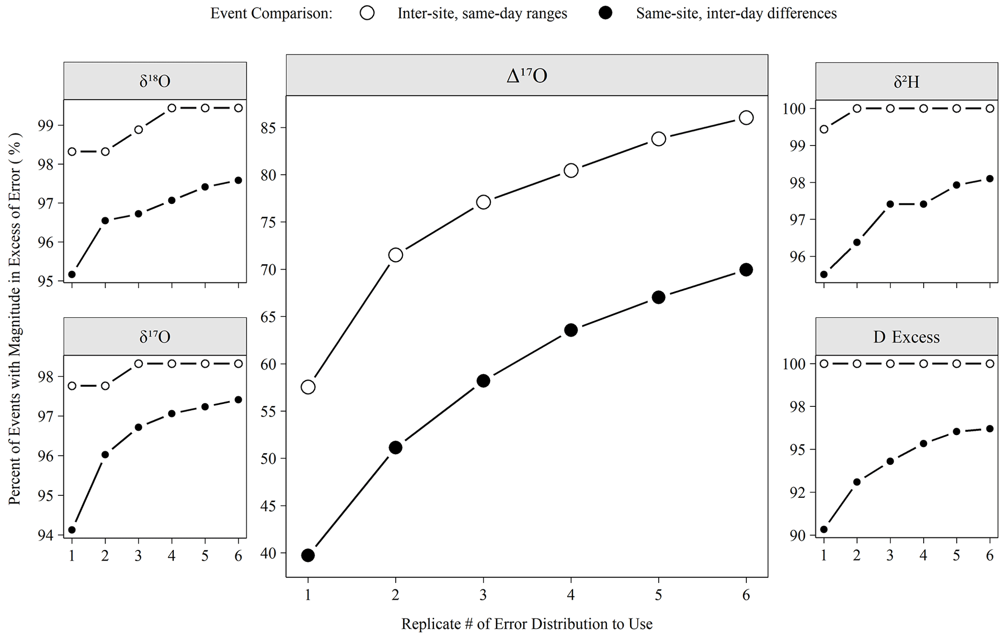
Figure 7 The percentage of meteoric precipitation events captured by varying numbers of analytical replicates. Inter-site, same-day ranges are the range of all sites from a Ugandan monitoring network (see Sect. 2.1). Same-site, inter-day differences are the differences of measured isotope values between sequential precipitation events (< 7 d span). If the event magnitude (either range or difference) exceeded the error for a given replicate number (Fig. 6), then it is considered here “detected”.

The number of replicates to perform is a critical operational choice as this sets the analytical throughput of the instrument. Figure 7 demonstrates the effect of replicate number on a potential scientific question. Utilizing the low-latitude precipitation samples that were the bulk of unknowns run during the period considered here, we defined two types of events that we might want to detect. Inter-site, same-day ranges are the range of isotope values observed at all sites with rain on a given day in the network, and same-site, inter-day differences are the difference of isotope values observed between consecutive (< 7 d apart) precipitation events at a single site. If the magnitude of the range or difference exceeded the replicate error structure shown in Fig. 6, then the event was detected. Figure 7 shows that a large majority of these events are readily detectable (i.e., exceed our error estimate) for any replicate number for all measurements except Δ¹⁷O. For Δ¹⁷O, an increase from 1 to 3 replicates allows for the detection of ∼ 15 % more events in absolute terms or 20 % (ranges) to 30 % (differences) in relative terms. Although the scientific importance of such events is another question to be investigated, these events must first be detected to study their importance.

4.5 Operational choices to optimize the performance of Δ¹⁷O, δ¹⁸O, δ²H, and d-excess in meteoric water samples using the Picarro L2140-i

Our results demonstrate that various operation modes and user choices for the Picarro L2140-i require trade-offs between data quality, time, effort, and/or training. Some operational choices that we describe above can optimize the performance of one measurement while degrading the quality or precluding measurement of another. For example, our limited experimentation suggests that normal mode results in better performance than ¹⁷O mode of δ¹⁸O but surprisingly slightly worse performance of δ²H and of course precludes analysis of Δ¹⁷O. Other user choices can clearly improve the performance of all isotope variables with only minimal additional time and effort, such as using high resolution for post-processing (see below), whereas other choices disproportionately improve some variables more than others, such as the approach to drift correction, so the decision to invest the extra time should depend on the scientific questions being investigated. That said, there are several operational choices that we contend are necessary for reliable and reproducible analysis of Δ¹⁷O, such as removal of organics. In this section, we offer recommendations for the particular use case of (1) analyzing predominantly natural, meteoric waters where large sample-to-sample differences are expected and (2) desiring optimal performance of Δ¹⁷O without sacrificing the quality of δ¹⁸O, δ²H, or d-excess. We expect this is a common use case for many laboratories wishing to incorporate Δ¹⁷O analyses into existing hydrologic, atmospheric, biological, and geological investigations based on stable isotopes in water or for new investigators wishing to analyze Δ¹⁷O in novel settings.

Corrections for memory, drift, and scale normalization. We contend that all of our corrections (memory, drift, and scale normalization) should be performed in order to optimize data quality. However, as discussed in Sect. 4.1, the number of drift standards could be reduced to a bracketed approach as long as some sacrifice to the performance of δ¹⁸O is acceptable to the user.

Long-pulse vs. high-precision mode. We recommend the increased analysis time of the long-pulse mode because it significantly improves precision for δ¹⁸O, δ¹⁷O, and Δ¹⁷O relative to the high-precision mode, consistent with Schauer et al. (2016). The shorter pulse lengths of the high-precision mode would require more replicates to match the performance of the long-pulse mode. While we do not have sufficient data from the high-precision mode to evaluate its error versus replicate pattern, if the pattern is similar to the long-pulse mode (Fig. 6) in that error is reduced as a function of the inverse root of the replicate number, then it would require ∼ 5 replicate analyses to achieve the same performance as our standard procedure of three replicates in the long-pulse mode. This would take approximately the same amount of analysis time but requires substantially more user preparation, uses more standard and sample material, and actuates the syringe much more often. As noted by others (Van Geldern and Barth, 2012; Schauer et al., 2016), syringe failure is by far the most common reason for sequence failure, and reducing the number of actuations is typically desired.

Processing data using high-resolution vs. coordinator streams. Although a post-processing choice and not an operation mode, we observed significant but essentially negligible improvements in precision for δ¹⁸O, δ¹⁷O, and Δ¹⁷O when processed using high-resolution versus coordinator outputs (see Sect. 2.3 for details on output types). However, high-resolution processing strongly outperforms coordinator data in terms of δ²H accuracy (∼ 0.25 ‰ RMSE improvement, Fig. S11), which is due to the shorter δ²H integration time that is made possible by working on the 1 Hz scale, high-resolution output that further reduces the impact of sample-to-sample memory (Schauer et al., 2016; Steig et al., 2014). Working with the high-resolution HDF files requires the use of some sort of command-line-based program capable of ingesting the HDF format (e.g., R, MATLAB, Python), as well as navigating the date–time-organized high-resolution folder structure. Combined, these make working with the high-resolution output more onerous than the much simpler, sequence-level summary CSV files of the coordinator output that can also be processed using available graphical user interface approaches (e.g., Coplen and Wassenaar, 2015; Gröning, 2011). The high-resolution output is also rich in additional diagnostic data streams such as the ability to calculate the more sensitive ¹⁸O laser flag spectral contamination metric (Fig. S2). Our unit has also exhibited occasional errant scans where only a single line (∼ 1 Hz) of high-resolution data has a poor spectral fit and extremely divergent isotope readings bounded by otherwise normal readings (Fig. S14). While we believe this particular problem may be unique to our unit, other unknown problems with these devices may be present and may only be detectable through analysis of the data-rich high-resolution files. In this specific case, the problem is both only detectable and solvable (the errant high-resolution data point is removed prior to calculation of the ∼ 560 high-resolution data point average for the injection) through the use of high-resolution data for post-processing. We do not recommend using coordinator output unless the worsened δ²H accuracy is acceptable.

Number and sequencing of replicate measurements. The replicate number should be determined based on the needed estimated accuracy of the measurement. Figure 6 is an effective guide, assuming similar long-term performance as our device. If your performance is better (or worse), then you should consider doing a similar analysis on your own data for more accurate estimates of error. We choose to distribute our unknown replicates across distinct sequences and recommend this approach to other users based on reasoning discussed in Sect. 4.2.

Removal of organic matter via the MCM. Our results using rainfall indicate that online removal of organic contaminants is mandatory to ensure data quality. Nearly 20 % of our samples (Fig. 4) exhibit symptoms of organic interference with much less (3 %) being detectable by spectral contamination flags, which is an experience confirmed by other users (Chang et al., 2016). Offline removal using activated charcoal or solid-phase extraction can remove some organic contaminants but typically remove only about 90 % of the starting concentration (Chang et al., 2016). This may be suitable for samples already near the limits of spectral interference (Fig. 3), although our limits are only for short-chain alcohols common in leaf extracts and may not represent organics found in rainfall. Future work on the concentration and specific identity of these contaminants will be useful in guiding strategies to handle organic inference for IRIS analysis.

5 Conclusions

In this work we present a measurement scheme and ∼ 2 years of analyses using a Picarro L2140-i to measure all the singly substituted stable isotopes of natural (predominantly meteoric) waters with a focus on optimized measurement of Δ¹⁷O. While isotope scale normalization is obviously mandatory, we find that our recommended post-processing corrections for instrumental drift and sample-to-sample memory strongly improve δ²H, δ¹⁷O, δ¹⁸O, and d-excess, whereas relatively little benefit is found for Δ¹⁷O. Critically, Δ¹⁷O is shown to be extremely sensitive to organic spectral interference, and this interference is often not detected by spectral contamination flags. The MCM is marketed by Picarro as an optional device, but the sensitivity of Δ¹⁷O to organics indicates that organic removal is required for confident measurement of any natural waters that may contain volatile organic carbon, including rainwater collected in field settings. However, the catalyst lifetime of MCM cartridges is quite variable, and there is no automatic indication of its failure. We resolve this by including a quality control standard intentionally spiked with interfering short-chain alcohols to ensure effective organic removal by the MCM.

We note that the uncertainty of Δ¹⁷O occupies a much larger fraction of its natural variability than other water isotope measurements. While our approach performs comparably with other laser-based devices (Pierchala et al., 2019; Schauer et al., 2016), we find that the variability of calibration bias for a sequence (Fig. 5) is a critical factor in producing accurate measurements of unknown samples. This is overcome by distributing replicates of unknown samples across distinctly calibrated sequences, and we measure this effect on accuracy empirically using control standards. For our recommended approach of three replicates, a total of ∼ 6.3 h per unknown sample is required, accounting for standards and inter-sequence downtime and yielding mean absolute errors of 0.3 ‰, 0.03 ‰, 0.02 ‰, 0.2 ‰, and 6 per meg for δ²H, δ¹⁸O, δ¹⁷O, d-excess, and Δ¹⁷O, respectively (Fig. 6). Due to replication, these are less than long-term RMSE (Table 2, Fig. 6). Our measurement approach and post-processing steps are applied in conjunction with modifications such as increased pulse length and shorter integration times of δ²H as described by Schauer et al. (2016).

Most of our recommendations are relatively easy to implement. For Δ¹⁷O, we find that most post-processing is unnecessary and that the only critical features for accurate and precise measurement are sufficient integration time (either by increased injections or longer pulses) and distribution of analytical replicates across distinctly calibrated sequences. Our finding of Δ¹⁷O organic sensitivity is specific to the L2140-i but, given similar spectra, likely impacts any infrared laser device. For overall performance of the instrument, we do find drift and memory corrections are necessary. While these post-processing steps can be onerous, memory correction removes the need to isotopically order samples. We document two avenues for data export from the instrument with appropriately matched processing scripts written in R. The use of the default coordinator output is more user-friendly than the HDF-based high-resolution stream, especially considering the compatibility with existing laboratory information management systems (Coplen and Wassenaar, 2015). The primary analytical benefit of high-resolution data is improved accuracy of δ²H. We provide standard operating procedures for post-processing complete with example data for both output types (supplemental files S1 and S2).

The recent 2020 water isotope intercomparison exercise (Wassenaar et al., 2021) clearly demonstrated the apparent difficulty of making accurate and precise Δ¹⁷O measurements by laser spectrometry. This difficulty was apparent even despite the lack of any organic-spiked samples included in the intercomparison set (employed in Wassenaar et al., 2018), which would have caused much more serious inter-lab deviations in Δ¹⁷O. Aside from organic interference, we demonstrate that the primary weakness of laser spectrometry Δ¹⁷O is sequence-level calibration bias. Our presented strategy overcomes this obstacle and yields comparable performance and throughput to DI-IRMS. This is achieved through a suite of operational parameters, sequence structure, and post-processing corrections, but we provide some options to ease adoption. Although the increased adoption of triple-oxygen-measuring laser spectrometry devices has expanded greatly in recent years, operator skill and care are required to produce robust Δ¹⁷O measurements that are competitive with DI-IRMS. The accessibility of laser spectrometry combined with careful operation will help to rapidly expand the study of the complete stable isotopic composition of water and enable the detection of signals previously hidden in the noise.