Observations of anomalous propagation over waters near Sweden

Radio waves propagating in the atmosphere are affected by the prevailing atmospheric state. The state of the atmosphere can cause radio waves to refract more or less towards the ground. When the refractive index of the atmosphere differs from standard atmospheric conditions, the propagation is considered to be anomalous. Radars which are affected by anomalous propagation can observe ground clutter far beyond the radar horizon. In this work, 4.5 years' worth of data from five operational Swedish C-band dual-polarization weather radars are presented. Analyses of the data reveal a strong seasonal cycle and a weaker diurnal cycle in ground clutter from coastal regions across nearby waters. A comparison was drawn between the impacts of anomalous propagation on ground clutter measured with horizontal polarization and vertical polarization, respectively; however, no clear difference was found.

1 Introduction

The atmosphere has a large impact on the propagation of electromagnetic waves. Radio waves are, for example, attenuated by precipitation, but due to the atmosphere's refractive property, radio waves are also refracted. The refractive index of the atmosphere depends on the temperature, pressure, and water vapor (Bean and Dutton, 1966; Battan, 1973; ITU, 2019). Due to the vertical inhomogeneity of the atmosphere, radio waves are normally refracted slightly towards the ground. One typical atmospheric state is referred to as the standard atmosphere (see, e.g., Patterson, 2008). However, other atmospheric conditions can also occur during which radio waves are refracted less (subrefraction) or more (super-refraction) towards the ground. In some cases, radio waves can even become trapped and reach the ground far beyond the normal radio horizon (for a description of the normal radio horizon, see, e.g., Skolnik (2001, chap. 8)). These non-standard atmospheric conditions lead to what is known as anomalous propagation (Battan, 1973; Turton et al., 1988).

The effects of anomalous propagation of radio waves were already known in the 1930s (Kerr, 1951). Since then, anomalous propagation has been studied thoroughly (see, e.g., Kerr, 1951; Bean and Dutton, 1966; Battan, 1973), and the research field is still active. For example, in order to better understand how the atmosphere's refractive index changes with height, a number of studies based on in situ measurements have been conducted. The refractive index has been measured at different heights using radiosondes (e.g., Steiner and Smith, 2002; Bech et al., 2002; Wang et al., 2018) or, less commonly, using instruments attached to towers or masts (Falodun and Ajewole, 2006; Adediji et al., 2011) or helicopters (Babin, 1996).

In situ measurements can achieve very high vertical resolution and, in some cases (e.g., measurements from towers or masts), high temporal resolution over long time periods. However, the horizontal resolution has so far been limited for in situ measurements. With the advancement of numerical weather prediction (NWP) models, a new way of investigating the atmosphere's refractive index has become available. von Engeln and Teixeira (2004) and Lopez (2009) used data from the European Centre for Mid-Range Weather Forecasting (ECMWF) to present global climatologies of the atmosphere's refractive index. Many more studies have used NWP data to examine the refractive index in more limited geographical regions (Atkinson and Zhu, 2006; Sirkova, 2015; Magaldi et al., 2016; Emmanuel et al., 2017). NWP data have been compared with radiosonde data, with which they have shown good agreement (von Engeln and Teixeira, 2004; Bech et al., 2007a; Zhu et al., 2022).

Anomalous propagation can have a large impact on radar measurements. If a radar beam is subjected to atmospheric subrefraction, targets close to the ground can be missed, whereas if a radar beam is super-refracted, unexpected ground clutter can occur far beyond the normal radar horizon. In addition to changes in the distances at which a target can be detected and increases in ground clutter, a range–height error can also occur (Skura, 1987). A range–height error can lead to an erroneous estimation of a target's true height. For the radar user, it is therefore important to know when and how often anomalous propagation conditions occur.

For weather radars, anomalous propagation often leads to unwanted ground clutter (Doviak and Zrnić, 2006). To address this problem, much work has been done to derive various algorithms that can detect and remove such echoes (see, e.g., Moszkowicz et al., 1994; Grecu and Krajewski, 2000; Cho et al., 2006; Overeem et al., 2020; Husnoo et al., 2021). Even though most studies concerning weather radars and anomalous propagation have focused on mitigating the effects of ground clutter, data from weather radars have also been used to study anomalous propagation itself. Fornasiero et al. (2006) analyzed 3 years' worth of data from two C-band dual-polarization weather radars in northern Italy and found a seasonal cycle and also a diurnal cycle in the received ground clutter. Increased occurrence of super-refraction was observed in the summer, as well as during nights and mornings. Mesnard and Sauvageot (2010) analyzed 1 year's worth of data from an S-band weather radar in southwest France. They reported on the spatial distribution and the temporal duration of continuous ground clutter detected far beyond the radar horizon from both sea and land.

Anomalous propagation is common in littoral environments (see, e.g., von Engeln and Teixeira, 2004). Even though Sweden is surrounded by waters (e.g., the Baltic Sea, the Gulf of Bothnia, and Kattegat), only a few studies on anomalous propagation based on data from this region have been published. Alberoni et al. (2001) proposed a method for removing ground clutter and sea clutter from weather radars and presented results from applying this technique on a few days' worth of data from a weather radar on the Swedish island of Gotland in the Baltic Sea. Bech et al. (2007b) investigated the effects of anomalous propagation on beam blockage models and, in a case study, applied their method to data from the same weather radar on Gotland. A number of measurement campaigns have also been conducted in the Baltic Sea, mainly focused on studying evaporation ducts. During these campaigns, a combination of in situ measurements, radiosondes, and microwave measurements were performed and reported (see, e.g., Scholz and Förster, 2003; Förster et al., 2004; Essen et al., 2004; Förster and Riechen, 2006; Essen et al., 2012; Danklmayer et al., 2013, 2015, 2016a, b).

Despite the large impact of anomalous atmospheric conditions on the propagation of radio waves, no long-term analyses of continuous radar measurements over the Baltic Sea or its neighboring waters have, as far as the author is aware, been published. A more thorough investigation of anomalous propagation in this region is therefore warranted. In this work, we present data from five Swedish weather radars from 2017 to 2021 in order to study the seasonal and diurnal cycles of anomalous propagation over the waters near Sweden.

2 Data

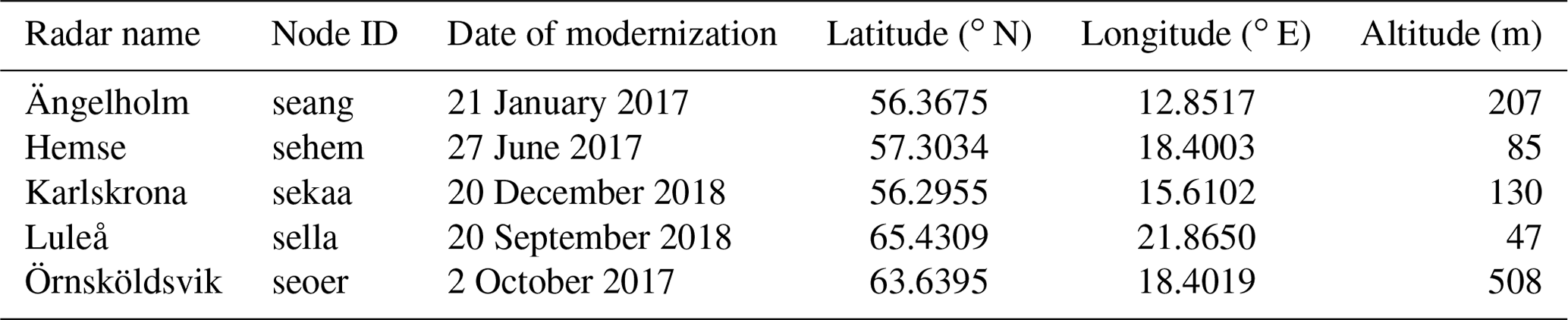
The Swedish weather radar network consists of 12 dual-polarization, C-band, Doppler weather radars. The radars provide almost-nationwide cover, with an update rate of 5 min. The current weather radars were recently modernized from single to dual polarization. The modernization dates for the radars that were used in this work are shown in Table 1.

Table 1 Location and modernization dates for the weather radars selected for this work.

Weather radars measure echo strength using the equivalent radar reflectivity factor Z (hereafter called reflectivity), which is expressed in mm⁶ m⁻³ or, in its corresponding logarithmic unit, dBZ (Doviak and Zrnić, 2006). The minimum echo strength the Swedish weather radars register is −32 dBZ. Any signal equal to or below the minimum echo strength is given this value. This echo value is later in this work referred to as “no echo”. At larger distances from the radars, the sensitivity is not enough to measure −32 dBZ. For example, at the maximum distance of 240 km, the minimum echo strength detected by the Swedish radars is approximately 10 dBZ. The maximum echo strength the radars record is 96 dBZ.

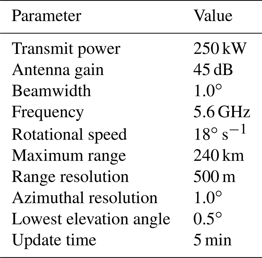
The scan strategy consists of 10 different elevation angles, with 0.5^∘ being the lowest elevation angle. The maximum unambiguous range for the lowest four elevation angles is 240 km. The radar data are stored with a range resolution of 500 m and have an azimuthal resolution of 1^∘. These and some other technical parameters of the radars are shown in Table 2. For more information on the radars, see the World Meteorological Organization weather radar database (WMO, 2023).

Table 2 Some of the technical parameters used by the Swedish weather radar systems.

According to the radar program of the European Meteorological Services Network (EUMETNET, 2023), weather radars should be identified by a five-letter node (Michelson et al., 2019). The node identifiers for the Swedish radars are shown in Table 1, as well as in Fig. 1. The node identifiers are used to refer to the different radars throughout the rest of this document.

The Swedish weather radars generate a range of products based on the received echoes. Two products have been used in this work: the unfiltered reflectivity data and the corresponding Doppler-filtered reflectivity data. Since the radars use dual polarization, the impact of anomalous propagation on polarization has also been studied. For this reason, data sets from both horizontal and vertical polarization were used. The weather radars use dual polarization in a simultaneous transmit-and-receive mode. All data in this work come from polar volumes, but only data from the scan with the lowest elevation angle, 0.5^∘, were analyzed. Data from 1 January 2017 until 20 July 2021 were used.

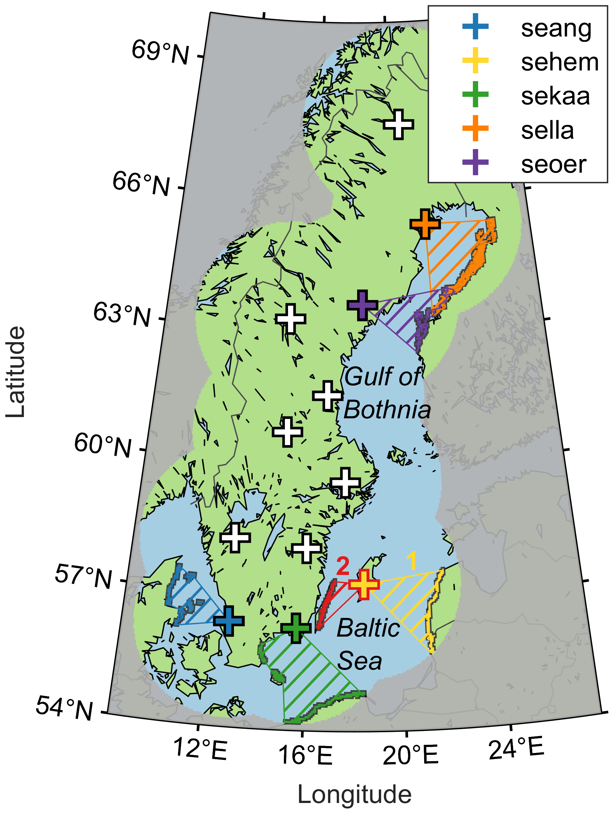
Figure 1 The Swedish weather radar network and its coverage. Radar locations are marked by plus signs. The five radars used in this work are listed in the legend. Six groups of radar cells from these five radars were selected to monitor for ground clutter. These radar cells are shown in different colors.

3 Method

3.1 Extracting ground clutter from weather radar data

As was mentioned in Sect. 2, the Swedish weather radars generate two products that are of interest for this study: the unfiltered reflectivity data and the Doppler-filtered reflectivity data. The Doppler-filtered data are useful for measuring precipitation rates, as this filter suppresses echoes from non-moving targets such as ground clutter. The Doppler-filtered data are the product that is of most interest to meteorological analyses. The unfiltered reflectivity data are useful for comparison and for troubleshooting but are otherwise normally of little interest for meteorological purposes.

In this work, we are, to the contrary, only interested in ground clutter and wish to suppress echoes originating from other sources. By subtracting the Doppler-filtered reflectivity data from the unfiltered reflectivity data, ground echoes can be extracted. In addition, many spurious signals, such as emissions from the sun or from man-made transmitters, can also be suppressed as long as these signals deviate sufficiently from the radar's own frequency.

Figure 2 shows reflectivity data from weather radar sehem, located on the island of Gotland in the Baltic Sea. The data presented in the figure have been averaged over the summer months (June, July, and August) from 2017 to 2021. Different panels in Fig. 2 show the unfiltered reflectivity data, the Doppler-filtered reflectivity data, and the difference between these two data sets.

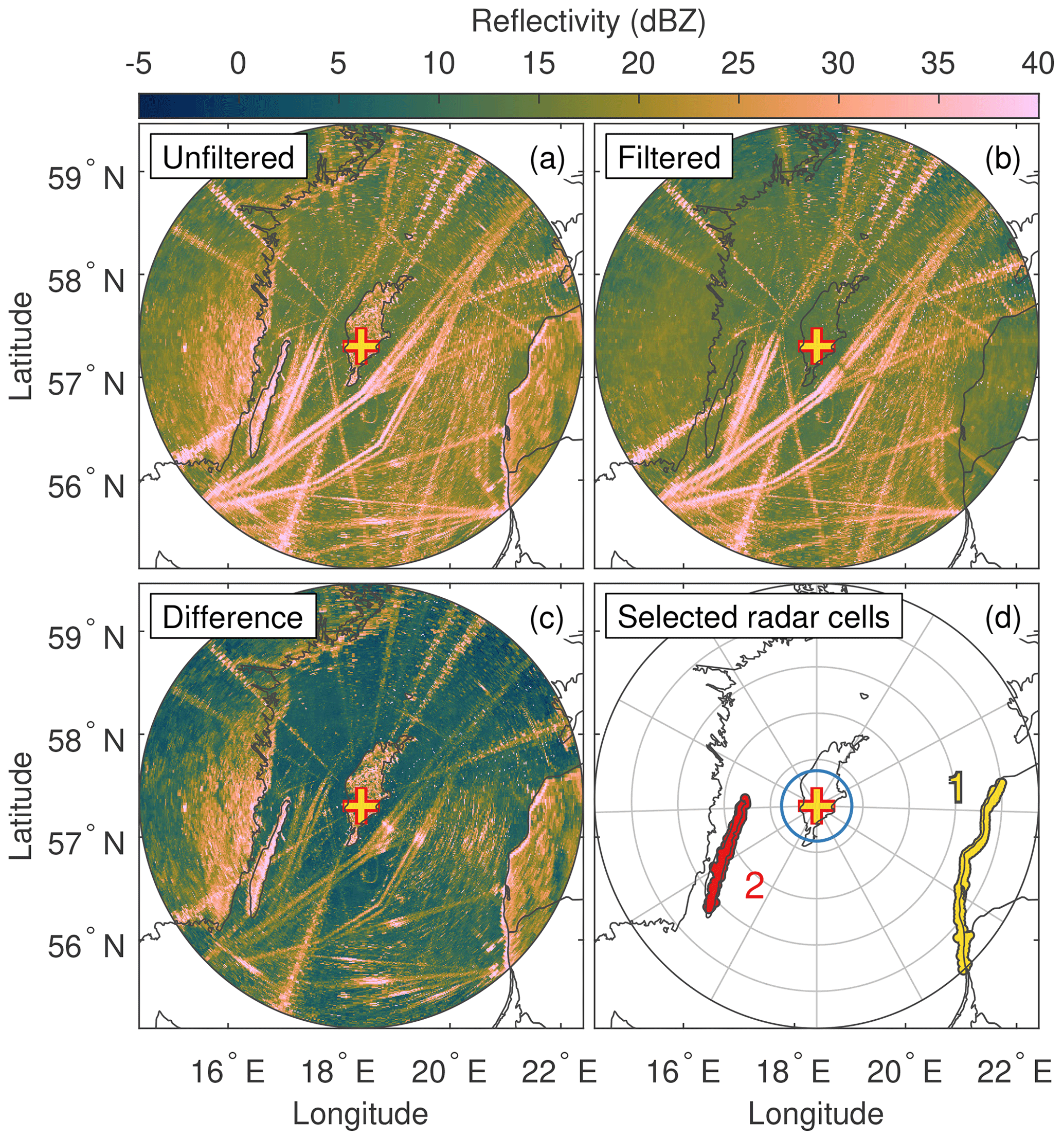
Figure 2 Data from weather radar sehem on the island of Gotland in the Baltic Sea, averaged over June, July, and August 2017–2021. (a) Unfiltered reflectivity data. (b) Doppler-filtered reflectivity data. (c) Difference between unfiltered and filtered reflectivity data. (d) Radar cells from two regions (the island of Öland to the southwest and the coastlines of Latvia and Lithuania to the east) were selected to study the effects of anomalous propagation. The blue ring near the radar shows the radar horizon, assuming standard atmospheric conditions. Range rings are displayed in 50 km increments.

Figure 2a shows the unfiltered reflectivity data. Here, the most prominent echoes originate from cargo ships, fishing vessels, etc. that regularly traffic the Baltic Sea. The ship routes are clearly seen, extending from the southwest to the northeast of the island. Strong echoes also come from ground clutter near the coastline of the Swedish island of Öland to the southwest and from the coastlines of Latvia and Lithuania to the east. Interference from other transmitters can also be seen, showing up as spokes from the edges to the radar at the center. In the background, a much weaker but more homogeneous echo can be seen. This background echo is the result of precipitation.

Figure 2b shows the Doppler-filtered reflectivity data. In this data set, much of the ground clutter from the coastal regions have been suppressed, but most of the ship echoes and interference from other transmitters still remain. However, when the radial velocities of the ships are close to zero, most of these echoes are suppressed. The precipitation background echoes remain in this data set.

Figure 2c shows the difference between unfiltered and filtered reflectivity data. From this data set, it is seen that the ground clutter from the coastlines are back. The echoes from the ships are suppressed (except when the radial velocities of the ships are close to zero). The background echoes from precipitation have also been reduced, while to a large degree, interference spokes from other transmitters still remain. This data set (the difference between the unfiltered and the Doppler-filtered reflectivity data) is used for further analyses.

Figure 2d shows two groups of radar cells that were selected for radar sehem for further study (see Sect. 3.2). The radar horizon, calculated for the center of the radar main lobe using standard atmospheric conditions, is also shown for comparison. It can be seen that all the selected radar cells are located well beyond the radar horizon.

3.2 Selecting radar cells to monitor for ground clutter

The radars that are of most interest for this study are radars that are situated near Sweden's coastline and for which land exists, within their maximum range, on the far side of nearby waters. Five radars were found to fulfill these conditions. These radars are shown in Fig. 1 and are also listed in Table 1.

For each of these radars, cells from the coastline of the far side of nearby waters were selected. The selected radar cells all showed large reflectivity values compared to neighboring radar cells when averaged over summer months (June to August; see Fig. 2). The selected radar cells are shown in Fig. 1. For the radar on the island of Gotland, sehem, radar cells were selected both to the east (the coastlines of Latvia and Lithuania) and to the west (the island of Öland).

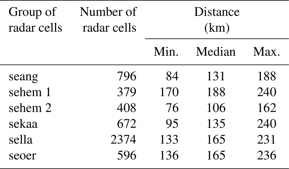
Table 3 lists the number of radar cells that were selected for each radar, together with the minimum, median, and maximum distances to these cells.

Table 3 Number of radar cells in the selected regions, together with minimum, median, and maximum distances to these cells.

3.3 Data analyses

In order to analyze the effects of anomalous propagation, the difference data set (see Sect. 3.1) was used. For all data analyses, the difference data set with horizontal polarization from the lowest elevation angle was used, unless otherwise stated.

From the difference data set, reflectivity values from the selected radar cells were extracted. For each group of radar cells, time series and histograms of the reflectivity data were generated. The time series were constructed by calculating the median reflectivity value from all radar cells in each group for every time step (i.e., with 5 min time resolution). In order to analyze the distribution of the reflectivity values, four different types of histogram were generated.

In the first type of histogram, the values of the reflectivity data from all the groups of radar cells were stored for each day of the year. Reflectivity data were binned with 0.5 dBZ resolution, i.e., stored in 256 bins. The histograms thus resulted in a matrix for each selected group with the size 365×256. From the histograms, empirical cumulative distribution functions (ECDFs) of reflectivity data were calculated for each day. In addition, time series of binary values were constructed, representing “echo” (reflectivity values $>-\mathrm{32}$ dBZ) or “no echo” (reflectivity value $=-\mathrm{32}$ dBZ).

In the second type of histogram, the values of all reflectivity data from all the groups of radar cells were stored as a function of the time of day (resulting in matrices with the size 288×256, i.e., the daily 5 min time resolution times the resolution of the binned data). In the same way as for the previous histograms, ECDFs were calculated for each time step of the day. Also, time series of binary values were constructed, representing “echo” or “no echo”.

In the third type of histogram, the relative frequency of echoes (i.e., reflectivity values $>-\mathrm{32}$ dBZ) for all groups of radar cells was calculated as a function of the day of the year and as a function of the time of the day (resulting in matrices with the size 365×288, i.e., the number of days of the year times the daily time resolution).

The fourth type of histogram consisted of pairwise reflectivity values from each of the three data sets (i.e., unfiltered, Doppler-filtered, and difference) using horizontal and vertical polarization. For each group of radar cells, the number of measurements with a certain horizontal reflectivity value and a certain vertical reflectivity value were stored (resulting in matrices with the size 256×256, i.e., the resolution of the binned data with horizontal polarization times the resolution of the binned data with vertical polarization).

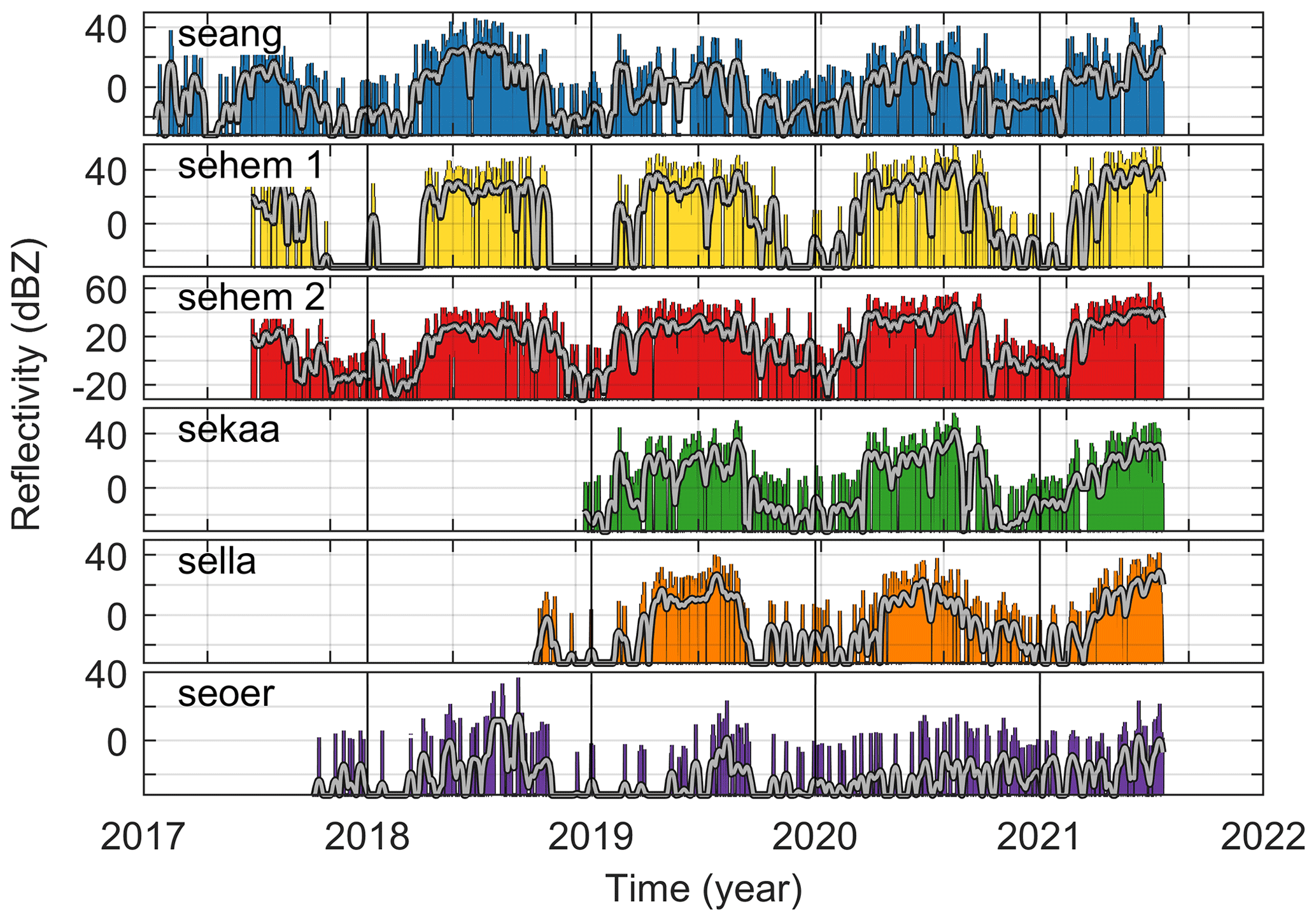
Figure 3 Time series of median values of reflectivity data from all selected groups of radar cells. Lines showing a moving average in time are depicted in gray.

4 Results

4.1 Seasonal variation in ground clutter strength

Using the time series that were extracted for each of the selected groups of radar cells, the reflectivity data as a function of time could be visualized. Figure 3 shows the median reflectivity values from the selected groups of radar cells as a function of the time of year together with a line depicting a moving average in time (achieved by applying a 14 d long Hanning weighted window). For many of the selected groups, a seasonal cycle can be seen, perhaps most notably for group sehem 1. The values of the reflectivity data are, for every selected group, on average, higher during the summer months (June, July, and August) compared to during the winter months (December, January, and February). In the figure, it can also be seen that the reflectivity data from group seoer are much lower than those from the other groups. This is most likely a result of radar seoer being situated at a much higher altitude compared to the other radars (see Table 1). For radar seoer to detect ground clutter from the far side of the Gulf of Bothnia, the atmospheric super-refraction must be much stronger than for the other radars.

Another way of examining the time series from the selected groups of radar cells for periodic patterns is to perform a spectral analysis. Spectral analyses of all time series, using the fast Fourier transform, are shown in Fig. 4. The 1-year period and the 1 d period are highlighted in the figure. All time series show a peak in the spectral amplitude at the 1-year period, but only a few show signs of a diurnal cycle. Even for the time series in which the diurnal cycle is discernible (e.g., group sekaa), it is much weaker compared to the seasonal cycle.

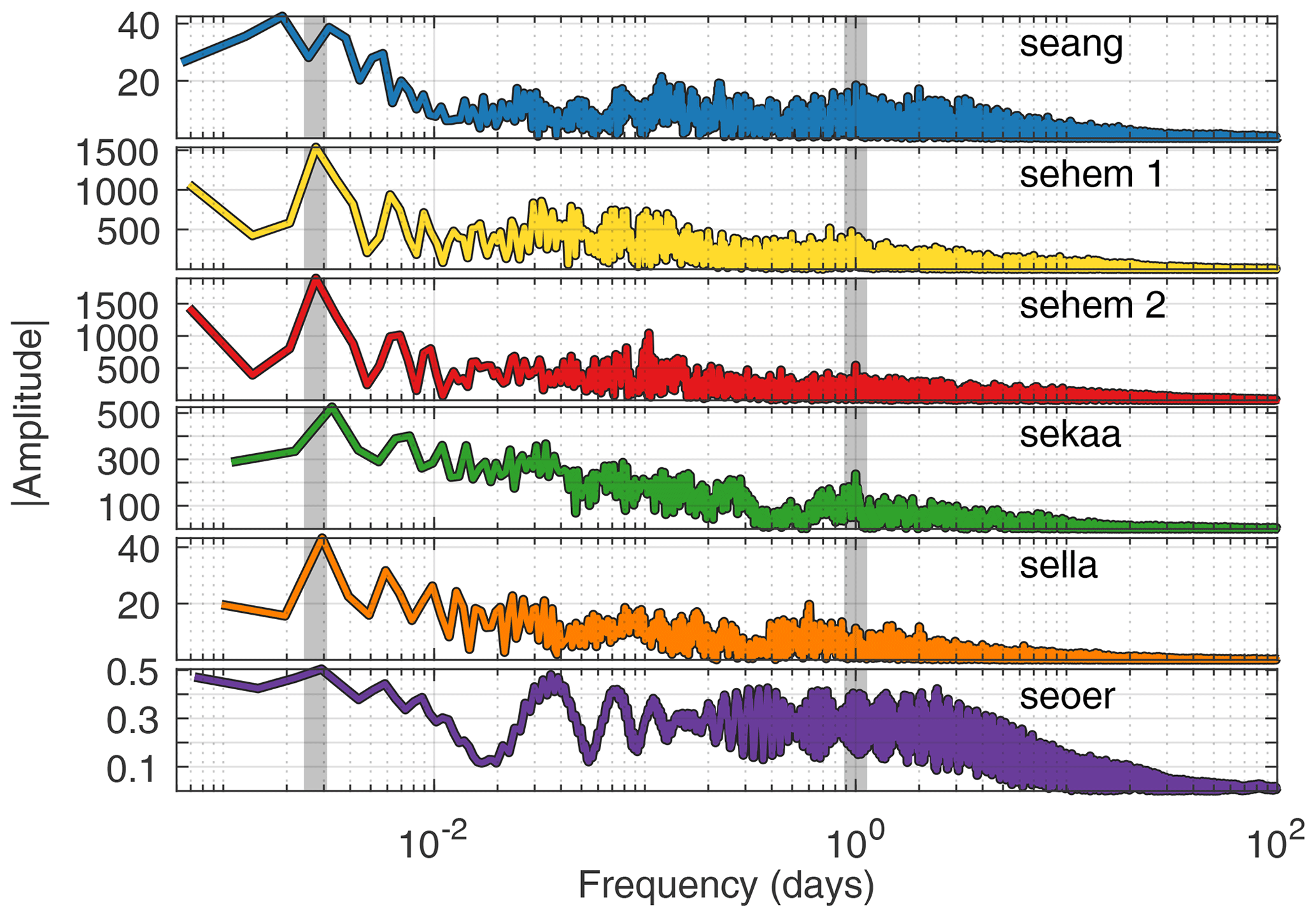
Figure 4 Spectral analysis of the median values of the reflectivity data from all radar cells in the selected areas. The 1-year and 1 d periods are highlighted in the figure with gray vertical lines.

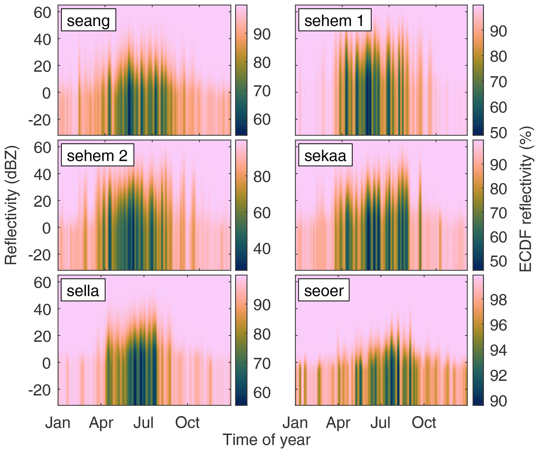
Figure 5 Empirical cumulative distribution function of reflectivity values from all selected groups of radar cells as a function of the time of year.

The time series only show median reflectivity values, and the seasonal cycle can be examined in greater detail by studying the histograms that were generated in the data analyses (see Sect. 3.3). Figure 5 shows the ECDFs of the reflectivity data as a function of the time of year for all selected groups of radar cells. In order to more clearly display the seasonal cycle, a moving average in time (achieved by applying a 7 d long Hanning weighted window) was applied to the data. From the figure, it is clear that an increase in reflectivity values occurs during the summer months but that most measurements still belong to the data bin with the lowest reflectivity value (i.e., −32 dBZ). This value, as explained in Sect. 2, actually shows that no echo of sufficient strength was detected. It can also be seen from Fig. 5 that radar seoer detects far fewer echoes from its selected group of radar cells compared to the other radars. For over 90 % of the time, there were no echoes detected by radar seoer from its selected radar cells.

In addition to examining the ECDFs of the reflectivity data, we can inspect the binary time series that represent “echo” or “no echo”. Figure 6 shows the relative frequency of detected echoes as a function of the time of year for all selected groups of radar cells. To more clearly show the seasonal cycle, a moving average was applied (using a 14 d long Hanning weighted window).

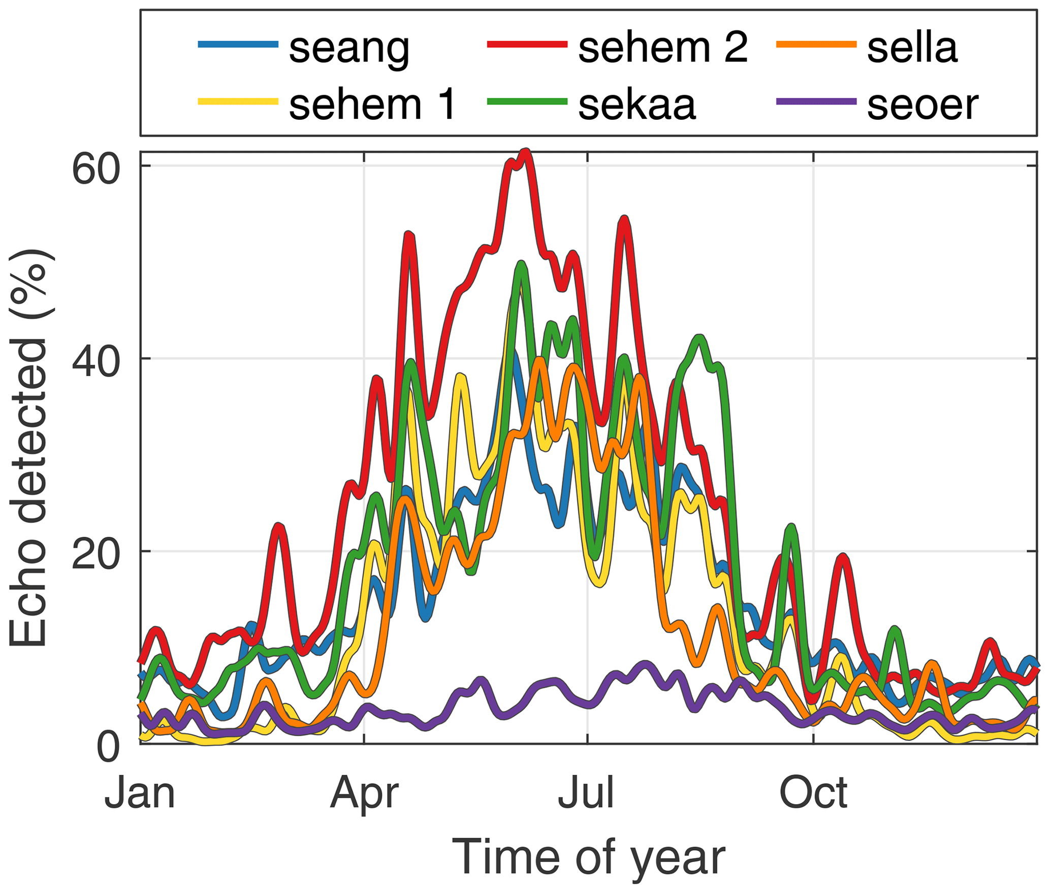
Figure 6 Relative frequency of detected echoes from the selected groups of radar cells as a function of the time of year.

From Fig. 6, it is clear that the chance of detecting ground clutter from the selected groups of radar cells increases during the summer months. This is true for all groups but is least clearly visible for group seoer due to the reason discussed above.

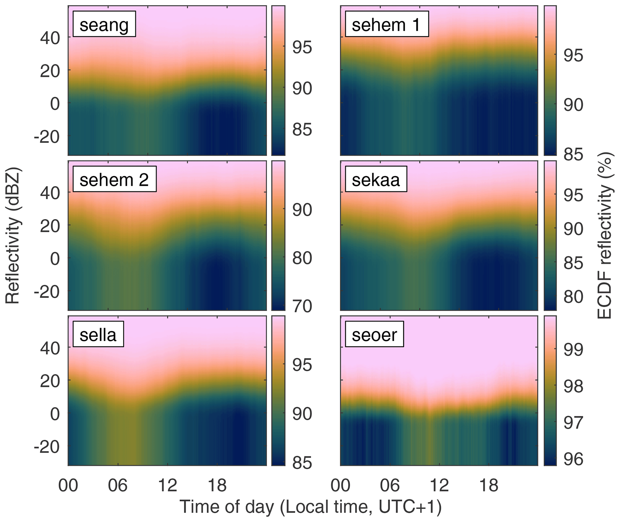
Figure 7 Empirical cumulative distribution function of reflectivity values for all selected groups of radar cells as a function of the time of day.

4.2 Diurnal variation in ground clutter strength

To investigate the extracted data for the presence of a diurnal cycle, the histogram that stored reflectivity values as a function of the time of day can be studied. In the same way as for the seasonal cycle, Fig. 7 shows the ECDFs of reflectivity data as a function of the time of day for all selected groups of radar cells. A weak but consistent diurnal cycle can be seen for all groups. The ECDFs show a decrease in stronger reflectivity values in the morning (around 06:00–07:00 local time, LT) and a slight increase in stronger reflectivity values in the evening (around 18:00–19:00 LT). It can also be seen that, for a majority of the time, no echoes were detected from any group of radar cells. This is particularly evident for echoes from group seoer, from which detectable echoes were observed less than 5 % of the time.

As for the analysis of the seasonal cycle, a binary value can be defined from the data, representing “echo” or “no echo”. The relative frequency of detected echoes as a function of the time of day is shown in Fig. 8. Here, the diurnal cycle is clearly visible for all groups of radar cells except for group seoer. Even for the other groups, echoes were only detected, on average, some 10 %–25 % of the time, and the variation during the day was of the order of 5 % or less.

4.3 Seasonal and diurnal variation in ground clutter strength

From Figs. 6 and 8, it is clear that there exists both a seasonal cycle and a diurnal cycle in the reflectivity data, extracted from the selected groups of radar cells. In order to separate the two cycles, Fig. 9 shows the relative frequency of detected echoes as a function of both the time of year and the time of day. To improve visibility, the data in the figure were smoothed over the time of year by applying a moving-average filter (using a 7 d long Hanning weighted window). No smoothing was applied to the time of day.

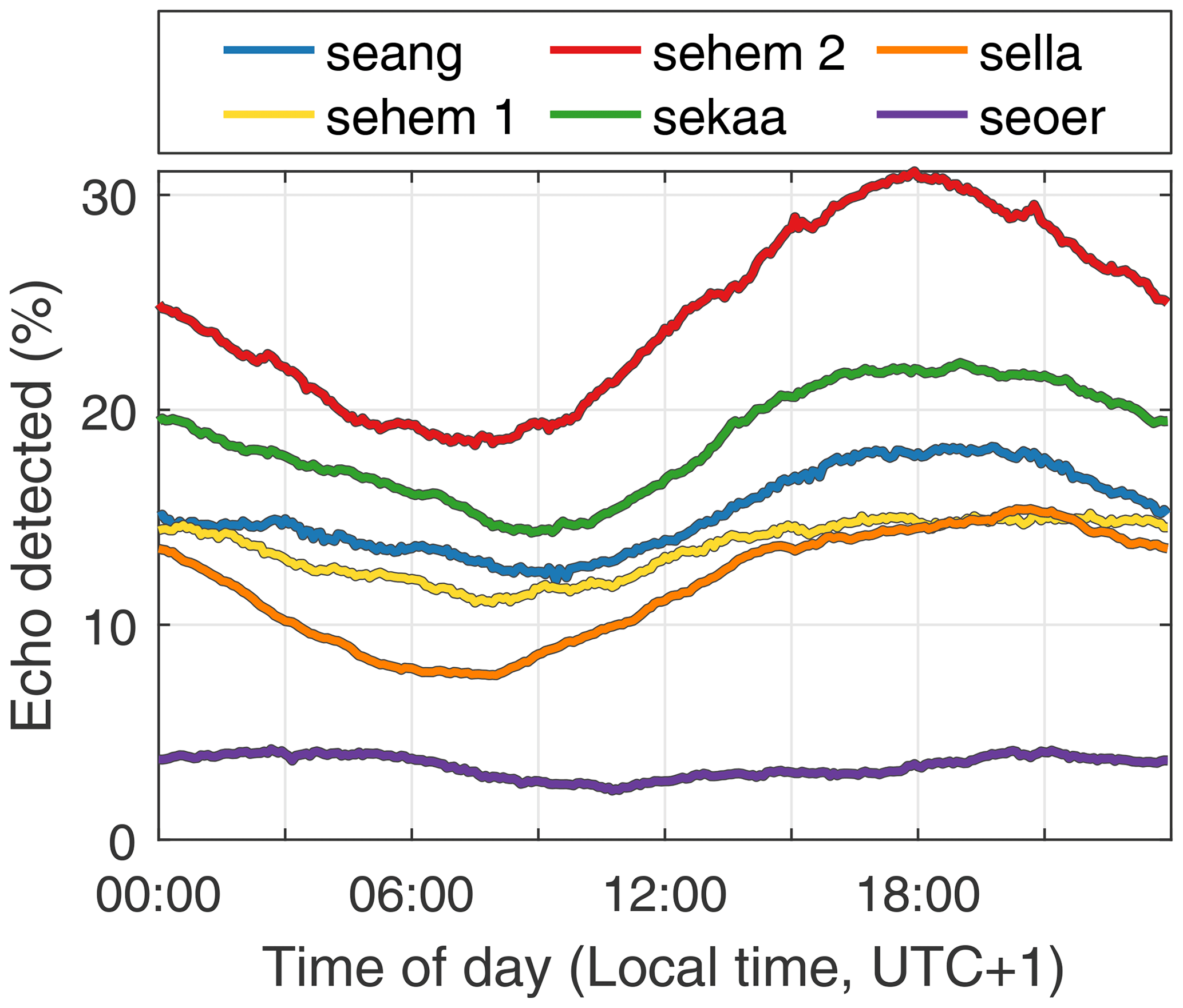
Figure 8 Relative frequency of detected echoes from all the selected groups of radar cells as a function of the time of day.

Figure 9 highlights the results that have already been shown. A prominent seasonal cycle is seen for all selected groups of radar cells (even though is it considerably weaker for group seoer). Most echoes occurred during summer, and echoes were clearly less common during winter. Imposed on the seasonal cycle, a diurnal cycle can be seen. Echoes were more frequently detected during the evening, around 18:00 LT. The fewest echoes were detected in the morning, around 06:00–07:00 LT.

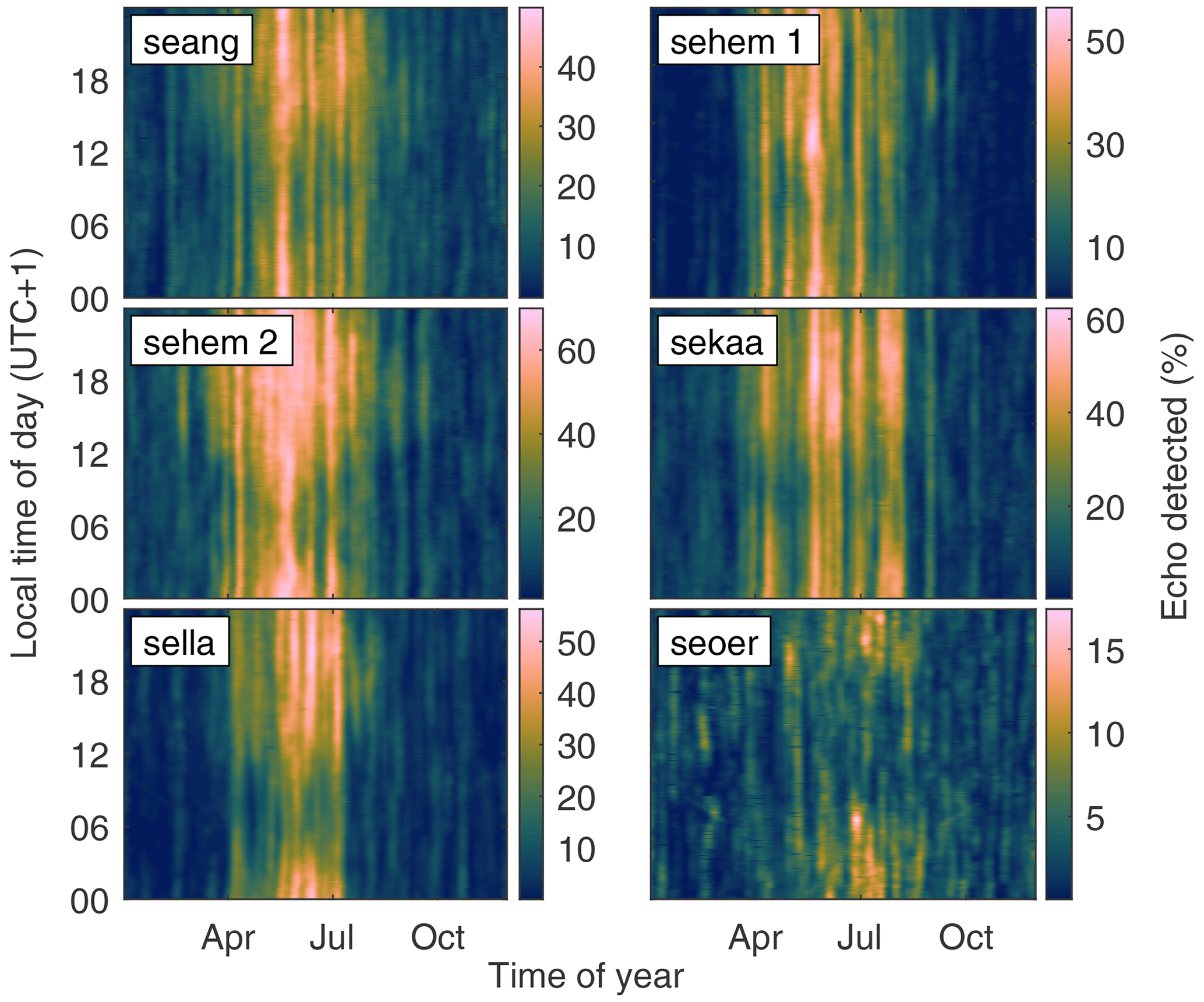
Figure 9 Relative frequency of detected echoes from all selected groups of radar cells as a function of the time of year and of the time of day.

4.4 Polarization and ground clutter strength

The results presented above were all based on measurements using horizontal polarization. In order to investigate whether ground echoes from a vertically polarized wave were affected by anomalous propagation in the same way, pairwise measurements of horizontal and vertical polarization were stored.

From the pairwise data set, two-dimensional histograms were generated for all selected groups of radar cells using the unfiltered data set, the Doppler-filtered data set, and the difference data set (see Sect. 3.1). The results are presented in Fig. 10. In the figure, the histograms for the three different data sets are shown together with relative frequencies of the difference between the reflectivity values of the two polarizations for all three data sets.

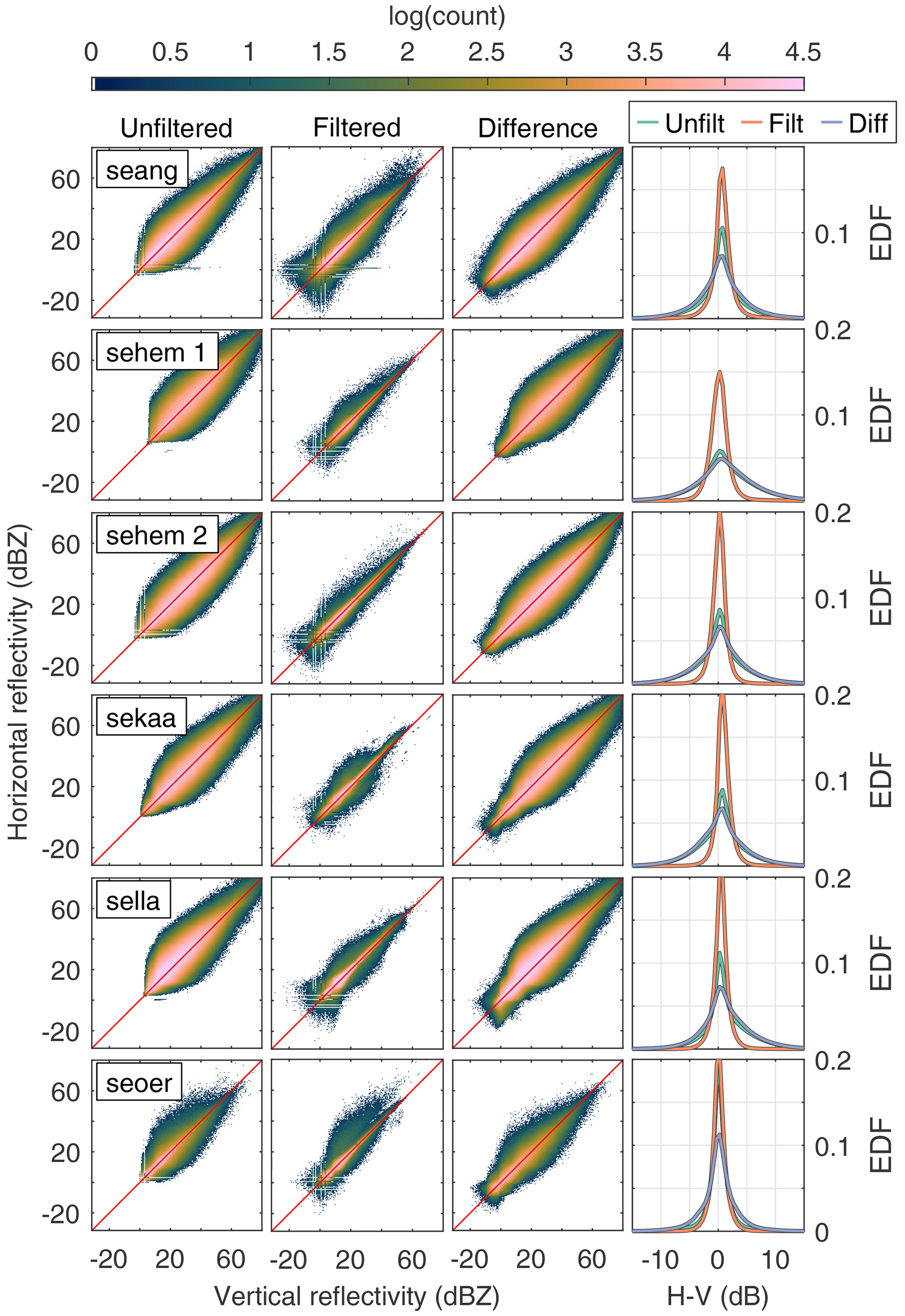
Figure 10 Columns 1–3 show histograms of pairwise measurements of reflectivity data using horizontal and vertical polarization for three different data sets: unfiltered reflectivity, Doppler-filtered reflectivity, and the difference between the unfiltered and filtered data sets. Column 4 shows empirical distribution functions of the pairwise difference between horizontal and vertical measurements.

It can be seen from the histograms that most of the data are concentrated along the diagonal line at which the horizontal and the vertical reflectivity values are equal. Some deviations can be seen, but the distributions are mostly symmetrical for all three data sets. Data from the Doppler-filtered data set are most closely concentrated along the diagonal line, which is true for all groups of radar cells. Since the main difference between the Doppler-filtered data set and the other two data sets (at the selected radar cells) consists of ground clutter, the implication is that ground clutter vary more than echoes from precipitation when using different polarizations. However, from the figure, it is difficult to tell if ground clutter from either polarization are stronger, on average.

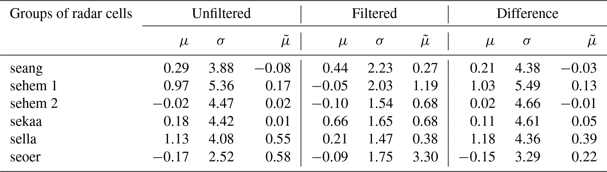
To find any systematic difference between the ground clutter reflectivity values from the two polarizations, statistical parameters were calculated from the pairwise data set. Table 4 lists the mean (μ), the standard deviation (σ), and the skewness $\left(\stackrel{\mathrm{̃}}{\mathit{\mu }}=E\left[{\left(x-\mathit{\mu }\right)}^{\mathrm{3}}/{\mathit{\sigma }}^{\mathrm{3}}\right]\right)$ of the pairwise data set for all selected groups of radar cells. The table emphasizes what can be seen in Fig. 10, namely that the standard deviations for the unfiltered and difference data sets are larger than the standard deviation for the Doppler-filtered data set. Ground clutter from horizontal polarization tends to result in slightly stronger reflectivity values compared to that from vertical polarization (up to ca. 1 dB). The Doppler-filtered data set has the largest skewness values, which are positive for all selected groups of radar cells.

Table 4 Statistical parameters for the difference in pairwise reflectivity values measured using horizontal and vertical polarization for all selected groups of radar cells and three different data sets. Mean values (μ) are in dB, standard deviation (σ) is in dB, and skewness ($\stackrel{\mathrm{̃}}{\mathit{\mu }}$) is unitless.

5 Discussion

In this work, data from operational weather radars have been used to analyze anomalous propagation. To do this, echoes from non-moving targets were extracted from radar cells in coastal areas on the far side of nearby waters. While it is not possible to know the radar cross-section of the ground in the selected radar cells, the relative changes in echo strength over time can be studied.

The assumption in this work is that the changes in ground clutter strength over time are due to changes in the atmospheric conditions and, in particular, to variations in the refractive index of the atmosphere between the radar and the selected radar cells. However, there are other factors that also can change and have an impact on the received echoes.

Precipitation attenuates radar waves and could affect the strength of the received ground clutter. However, since precipitation in the studied region is generally higher during the summer and is often in form of snow in the winter (which leads to weaker reflected echoes), the seasonal cycle should actually be more pronounced if this was taken into consideration.

For the period of the study (2017–2021), the Gulf of Bothnia (see Fig. 1) was ice covered in the winter for 4 of the 5 years. The radar most significantly affected by the ice cover was radar sella. A more detailed analysis of how the ice cover affects the atmospheric conditions would be interesting to conduct but is out of scope of this work.

There are some limitations in using the presented method. While analyzing the variation in ground clutter over time provides an understanding of how the radars are affected by anomalous propagation, it is not possible to extract the horizontal distribution of the atmospheric refraction. Ground clutter only reveals the total impact, but it is quite possible that the refraction is inhomogeneous.

Another limitation in using this method is that it is not possible to account for the presence of subrefraction, at least not for the long distances studied here. As the weather radar should not detect ground clutter from far beyond the radar horizon during standard atmospheric conditions, there should be no difference in the received ground clutter during subrefractive conditions.

The results presented in this work could be used to compare with atmospheric refractive indices extracted from NWP data if used together with a radio wave propagation model. The results could also be compared to other data sets from the same region. It would be especially interesting to compare the presented data with a data set based on another frequency, such as data from X-band radars or communication signals on the VHF band.

6 Conclusions

In this work, 4.5 years' worth of data from operational weather radars in Sweden have been used to analyze anomalous propagation. Five radars situated close to the Swedish coast were selected for this study. From these radars, radar cells from six coastal regions from the far side of nearby waters were selected. The temporal variations in the received ground clutter from these regions were analyzed.

The analyses show that a clear seasonal cycle exists in the extracted reflectivity data. During summer months (June, July, and August), ground clutter were more frequent and also stronger, whereas during winter (December, January, and February), ground clutter were less frequent and much weaker.

In addition to the seasonal cycle, a diurnal cycle was found. The diurnal cycle was much weaker than the seasonal cycle, but it was nevertheless found that ground clutter were more frequent (and stronger) in the evening (around 18:00 LT) and less prevalent (and also weaker) in the morning (around 06:00–07:00 LT).

Since the weather radars utilize dual polarization, the data set was examined for any systematic difference between reflectivity data from horizontal and vertical polarizations. In the examined data set, reflectivity data from horizontal polarization were slightly stronger (up to approximately 1 dB) than reflectivity data from vertical polarization.