the Creative Commons Attribution 4.0 License.
the Creative Commons Attribution 4.0 License.
 | 12 Apr 2023
Ground-based remote sensing of aerosol properties using high-resolution infrared emission and lidar observations in the High Arctic
Denghui Ji
Mathias Palm
Christoph Ritter
Philipp Richter
Xiaoyu Sun
Matthias Buschmann
Justus Notholt
Arctic amplification, the phenomenon that the Arctic is warming faster than the global mean, is still not fully understood. The Transregional Collaborative Research Centre “TRR 172: ArctiC Amplification: Climate Relevant Atmospheric and SurfaCe Processes, and Feedback Mechanisms (AC)3” program, funded by the Deutsche Forschungsgemeinschaft (DFG, German Research Foundation), contributes towards this research topic. For the purpose of measuring aerosol components, a Fourier transform infrared spectrometer (FTIR), for measuring downwelling emission (in operation since 2019), and a Raman lidar are operated at the joint Alfred Wegener Institute for Polar and Marine Research and Paul Emile Victor Institute (AWIPEV) research base in Ny-Ålesund, Spitsbergen (79∘ N, 12∘ E). To carry out aerosol retrieval using measurements from the FTS, the LBLDIS retrieval algorithm, based on a combination of the Line-by-Line Radiative Transfer Model (LBLRTM) and the DIScrete Ordinate Radiative Transfer (DISORT) algorithm, is modified for different aerosol types (dust, sea salt, black carbon, and sulfate), aerosol optical depth (AOD), and effective radius (Reff). Using lidar measurement, an aerosol and cloud classification method is developed to provide basic information about the distribution of aerosols or clouds in the atmosphere and is used as an indicator to perform aerosol or cloud retrievals with the FTS. Therefore, a two-instrument joint-observation scheme is designed and subsequently used on the data measured from 2019 to the present. In order to introduce this measurement technique in detail, an aerosol-only case study is presented using data from 10 June 2020. In the aerosol-only case, the retrieval results show that sulfate is the dominant aerosol throughout the day ( = 0.007 ± 0.0027), followed by dust ( = 0.0039 ± 0.0029) and black carbon ( = 0.0017 ± 0.0007). Sea salt ( = 0.0012 ± 0.0002), which has the weakest emission ability in the infrared wave band, shows the lowest AOD value. Such proportions of sulfate, dust, and BC also show good agreement with Modern-Era Retrospective analysis for Research and Applications version 2 (MERRA-2) reanalysis data. Additionally, comparison with a Sun photometer (AErosol RObotic NETwork – AERONET) shows the daily variation in the AOD retrieved from FTS to be similar to that retrieved by Sun photometer. Using this method, long-term observations (from April to August 2020) are retrieved and presented. We find that sulfate is often present in the Arctic; it is higher in spring and lower in summer. Similarly, BC is also frequently observed in the Arctic, with less obvious seasonal variation than sulfate. A BC outburst event is observed each spring and summer. In spring, sulfate and BC are dominant, whereas sea salt and dust are relatively low. In addition, a sea salt enhancement event is observed in summertime, which might be due to the melting of sea ice and emissions from nearby open water. From the retrieved results over a long time period, no clear correlations are found; thus, the aforementioned species can be retrieved independently of one another.
- Article
(2854 KB) - Full-text XML
- BibTeX
- EndNote


In the Arctic, near-surface temperatures are rising much faster than those of the global mean (Wendisch et al., 2017). This phenomenon is called Arctic amplification (Serreze and Barry, 2011; Wendisch et al., 2017; Previdi et al., 2021). In order to understand the causes and effects of rapid warming in the Arctic, many studies have focused on the key processes contributing to Arctic amplification, like temperature feedback (Bony et al., 2006; Soden and Held, 2006), surface albedo feedback (Graversen et al., 2014), and cloud and water vapor feedback (Taylor et al., 2013; Philipp et al., 2020). The “TRR 172: ArctiC Amplification: Climate Relevant Atmospheric and SurfaCe Processes, and Feedback Mechanisms (AC)3” collaborative research program focuses on Arctic amplification (http://www.ac3-tr.de, last access: 6 December 2022).
Apart from the physical feedback processes, aerosol has a large impact on the Arctic environment (Abbatt et al., 2019; Schmale et al., 2021). Aerosol influences the Arctic climate via aerosol–cloud interactions (Fan et al., 2016) and aerosol–surface interactions (Donth et al., 2020). For example, black carbon (BC) deposits on snow and ice, lowering the surface albedo (Ming et al., 2009; Bond et al., 2013) and thus warming the surface. Dust, when present in layers over high-albedo surfaces and/or deposited to the snow, will warm the atmosphere (Krinner et al., 2006). In contrast, sulfate, organic matter, and sea salt may cool the Arctic by scattering light back to space and by modifying the microphysics of liquid clouds (Schmeisser et al., 2018). At cirrus temperatures, dust, ammonium sulfate, and sea salt increase the cloud albedo by increasing ice crystal concentrations (Wagner et al., 2018).
In recent decades, mainly in situ measurements of aerosols have been performed in the Arctic. Most reports show that the aerosol composition is changing. Koch et al. (2011) and Ren et al. (2020) found that sulfate and BC are decreasing compared with the last century. Several projects in the aforementioned ArctiC Amplification: Climate Relevant Atmospheric and SurfaCe Processes, and Feedback Mechanisms (AC)3 collaborative research program also focus on BC concentration measurements (Kodros et al., 2018; Zanatta et al., 2018), and they have revealed an annual cycle of BC in the Arctic: higher concentrations in spring and lower concentrations in early summer (Schulz et al., 2019). Shaw (1995) and Francis et al. (2018, 2019) found that dust can be transported over long distances into the Arctic and that this process plays an important role in Arctic haze. In recent years, the open-water area has become larger and the sea surface temperature has increased, leading to a local increase in the emission of sea salt (Domine et al., 2004; Struthers et al., 2011; May et al., 2016). Thus, during the Arctic warming period, the proportions of different aerosols in the region also change.
There are several ways to measure the aerosol composition, including remote sensing from satellite or ground-based instruments, in situ measurements on the surface, or measurements from aircraft. Satellite instruments can provide measurements over large areas, but they are not very suitable in the Arctic due to the frequent existence of clouds and snow/ice on the surface, which make measurements challenging (Lee et al., 2021). In situ measurements provide much more accurate information, but they are often limited to the planetary boundary layer, have limited coverage, and are temporally sparse. Ground-based remote sensing provides measurements with a similar measurement geometry to those of satellites and is not confined to a particular altitude, unlike in situ measurements. Ground-based methods provide time series measurements from the surface and have a similar viewing geometry to satellites. Hence, a combination of different measurement methods is necessary to provide a complete picture of aerosols in the Arctic. In this paper, we focus on a passive ground-based remote sensing method in the thermal infrared region in order to retrieve the aerosol components. Using atmospheric thermal emission spectra, measured by a Fourier transform spectrometer (FTS), we perform a retrieval of aerosol properties as proposed by Rathke et al. (2002). Turner (2008) extended this method to dust measurements. However, these previous studies (Rathke et al., 2002; Turner, 2008) were limited to a specific type of aerosol, such as sulfate or dust. Based on the aforementioned publications, this paper will further expand the number of aerosol types that can be measured by FTS.
The remainder of this paper is structured as follows: in Sect. 2, the measurement site location and the setup of the two instruments are described; Sect. 3 presents the joint-observation scheme using two instruments, the Koldewey Aerosol Raman Lidar (KARL) and the NYAEM-FTS Fourier transform spectrometer, and information on the retrieval algorithm for the NYAEM-FTS, including details on the lookup tables of aerosol scattering properties; Sect. 4 presents the results of both the KARL and NYAEM-FTS measurements for one case study of an aerosol-only event (10 June 2020) and for long-term observations from April to August in 2020; and the article ends with a summary and conclusions in Sect. 5.
2.1 Site description
Ny-Ålesund (79∘ N, 12∘ E), Svalbard, is located in the North Atlantic atmospheric transport gateway to the Arctic. The AWIPEV (http://www.awipev.eu, last access: 6 December 2022) research base is part of the village of Ny-Ålesund and is jointly operated by the AWI Potsdam (Alfred Wegener Institute; http://www.awi.de, last access: 6 December 2022) and the IPEV (Polar Institute Paul-Émile Victor; https://institut-polaire.fr/, last access: 6 December 2022). The AWI Potsdam operates an extensive suite of instruments, some of which are a very useful complement to the NYAEM-FTS (Sect. 2.2), including an aerosol lidar instrument (Sect. 2.3) and a Sun photometer (Sect. 3.2).
2.2 The NYAEM-FTS instrument
The NYAEM-FTS Fourier transform spectrometer, which measures downwelling emission in the thermal infrared, was installed in summer 2019. The NYAEM-FTS consists of a Bruker VERTEX 80 Fourier transform spectrometer, an SR-800 blackbody, an automatically operated mirror to select the radiation source, and an automatically operated hutch that shields the instrument from the environment. It is situated in a temperature-stabilized (at about 21–25 ∘C) laboratory.
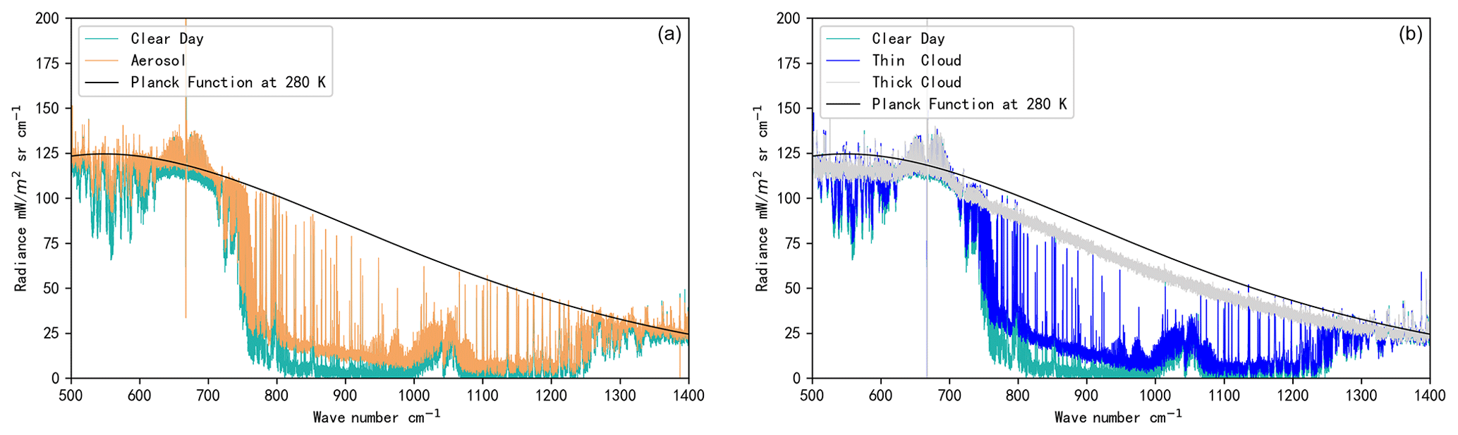
Figure 1Four different emission spectra measured by the NYAEM-FTS under (a, b) clear-sky (green), (a) aerosol event (yellow), (b) thin-cloud (blue), and (b) thick-cloud (gray) conditions, respectively. The radiance calculated using Planck function at 280 K (black line) is presented in this figure. Note that the emission at around 650 cm−1 originates under ambient CO2 conditions from the laboratory air.
The Bruker VERTEX 80 is a tabletop instrument. It is operated in zenith geometry with an adjustable field of view in the range of 3.3–22 mrad. The beam splitter is a KBr beam splitter, and the detector is an extended MCT (mercury–cadmium–telluride) detector with a spectral range of 400–2500 cm−1 (4–25 µm). This instrument has a spectral resolution of 0.08 cm−1 (August 2019–August 2020) or 0.3 cm−1 (August 2020 to the present). All resolutions are suitable for the analysis of aerosol properties, as the spectral features are broadband (see Fig. 1). The mirror selecting the emission source is the first optical part of the setup, and a total power calibration is performed to gain the radiance from spectra (Revercomb et al., 1988). This means that three measurements are required to complete the observation of a spectrum: two measurements of the blackbody at hot and ambient temperatures, respectively, and one measurement pointing skywards (Rathke and Fischer, 2000; Turner, 2005; Richter et al., 2022). The SR-800 blackbody is used as a blackbody radiator. It can be adjusted between 0 and 120 ∘C, holding the temperature within 0.1 K.
Figure 1 shows four different emission spectra measured by the NYAEM-FTS under clear-day, thick-cloud, thin-cloud and aerosol event conditions, respectively. The Planck function at 280 K is also presented in this figure. From Fig. 1, the intensity of thick-cloud emission in the infrared is high (close to that calculated using the Planck function). However, in the atmospheric window between 800 and 1200 cm−1, the intensity of clear-sky emission is lower (close to zero) than that of thick cloud. Between the thick-cloud and clear-sky emission spectra in this window (800–1200 cm−1), aerosol (Fig. 1 orange line) and thin-cloud (Fig. 1 blue line) emission spectra are presented as well, showing the baseline from which the aerosol information will be retrieved. In general, it is easy to distinguish between a thick-cloud and a clear-sky spectrum; however, distinguishing aerosols from thin cloud is difficult or impossible. Therefore, more information from other instruments, e.g., lidar measurements, is used to distinguish days with clouds from days with aerosols present above the instrument.
2.3 The Koldewey Aerosol Raman Lidar (KARL)
In Ny-Ålesund, the KARL is operated, and it measures in three colors (355, 532, and 1064 nm) (Ritter et al., 2016). It is positioned about 10 m away from the NYAEM-FTS and also points skywards. Aerosol backscatter coefficients (in all three colors), extinction coefficients (355 and 532 nm), and depolarization (355 and 532 nm) are measured.
Table 1Aerosol classification by lidar measurements, as per the classification system defined by Ritter et al. (2016).
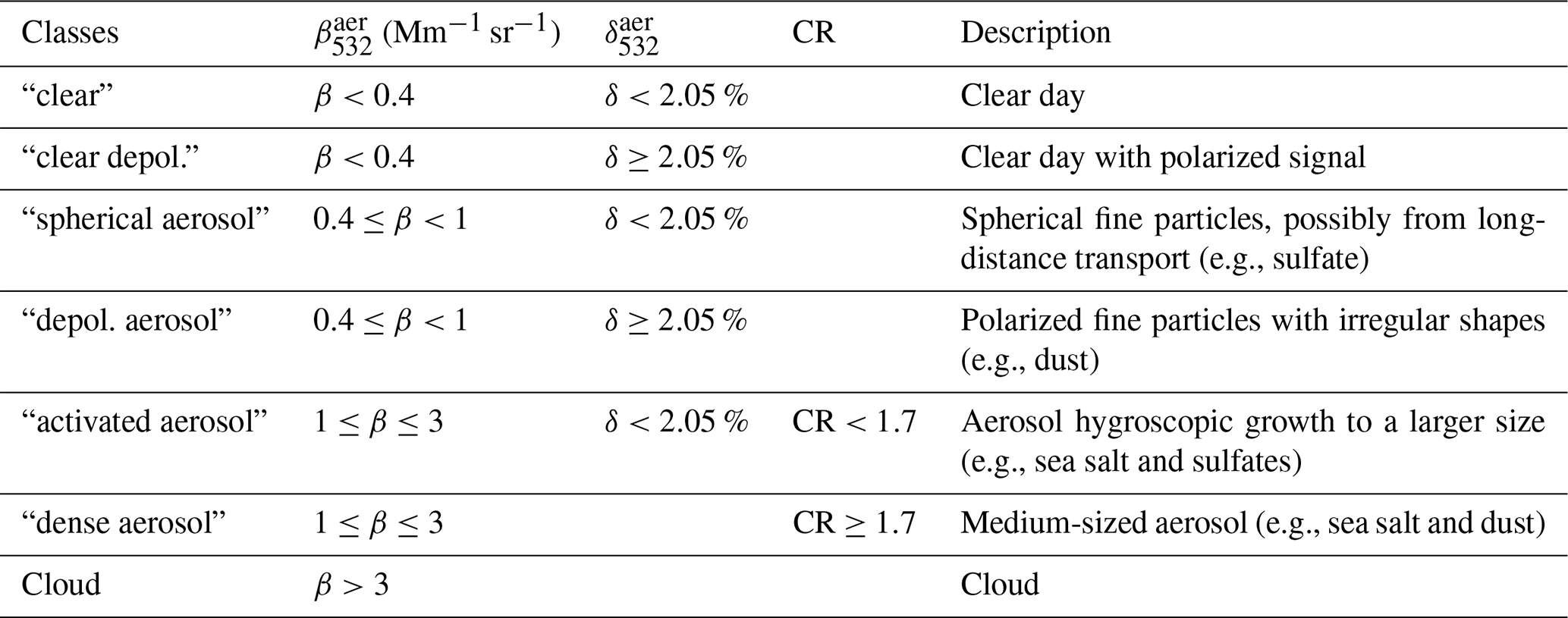
For lidar products, the aerosol backscatter coefficient (βaer), the aerosol depolarization (δaer), and the color ratio (CR) are used for aerosol optical property analysis. According to Freudenthaler et al. (2009), the definitions of those quantities are given as follows:
where and are the backscatter coefficients of the vertical and parallel polarized light, respectively. The depolarization depends on the particles' shape, e.g., spherical particles do not show any depolarization in the backscatter.
where is the aerosol backscatter coefficient at wavelength λ. More details are given in Freudenthaler et al. (2009) and Ritter et al. (2016). Based on the aforementioned information, Ritter et al. (2016) distinguished six conditions for the aerosol classification using those lidar quantities (see the conditions given in quotation marks in Table 1).
3.1 The TCWret V1 and TCWret V2 retrieval algorithms
The TCWret V1 and TCWret V2 retrieval algorithms are based on the Total Cloud Water retrieval (TCWret) algorithm developed by Richter et al. (2022). TCWret V1 is used for cloud parameter retrieval, whereas TCWret V2 is modified for aerosol retrieval. The main difference between the two is the scattering property lookup tables. The core of the TCWret retrieval program is the LBLDIS radiative transfer model (Richter et al., 2022), which consists of the Line-by-Line Radiative Transfer Model (LBLRTM) clear-sky radiative transfer model (Clough et al., 2005) and the DIScrete Ordinate Radiative Transfer (DISORT) scattering code (Stamnes et al., 1988). The LBLDIS coupled model is used in several retrieval algorithms, such as the mixed-phase cloud property retrieval algorithm (MIXCRA; Turner, 2005), CLARRA (Rowe et al., 2013), and TCWret (Richter et al., 2022). Note that these retrieval algorithms share the same forward models. The differences among them are the particular implementation, e.g., of the scattering.
In this paper, TCWret V1 refers to TCWret with cloud databases, whereas TCWret V2 refers to TCWret with aerosol databases. The algorithm reliability, or how well the method can precisely retrieve aerosol information, is tested in Sect. 3.1.4. In Sect. 3.1.1, the aerosol scattering property lookup tables and the artificial spectra simulated using the forward model are described in detail. A description of the retrieval algorithm can be found in Appendix A.
3.1.1 Aerosol scattering property lookup tables
In this study, sulfate, sea salt, dust, and BC are retrieved using the TCWret V2 retrieval algorithm. The complex refractive index database only covers the abovementioned aerosols in the infrared band. The spectral signature of the other aerosols is too small; thus, is not possible to retrieve them from the infrared (IR) spectra. The complex imaginary refractive indices of sulfate and dust are based on the Optical Properties of Aerosols and Clouds (OPAC) Global Aerosol Data Set (GADS), BC is from Chang and Charalampopoulos (1990), and sea salt is from Eldridge and Palik (1997) and Palik (1997) (see Fig. 3).
The aerosol optical properties are calculated using the Lorenz–Mie theory. The code for this calculation was developed by Mishchenko et al. (1999). For aerosol scattering property calculations, information on the aerosol size distribution and aerosol shape is also needed. In Mie code (Mishchenko et al., 1999), a spherical aerosol shape with a single-mode lognormal particle size distribution is selected. The lognormal function is given as follows:
where N is the total aerosol number concentration, Dg is the median diameter, and σg is termed geometric standard deviation. In this study, the geometric standard deviation of the aerosol size distribution is assumed to be 0.2, and the effective radius (Reff) is set from 0.1 to 1 µm. The main reason for setting the upper limit of the Reff to 1 µm is that aerosols in the Arctic region often have an Reff below 1 µm, according to measurements of the aerosol size distribution in the Arctic area (Asmi et al., 2016; Park et al., 2020; Boyer et al., 2023). In addition, if this constraint is not set to 1 µm, the retrieval of fine particles, such as sulfate and BC, will occasionally be mathematically increased for a better fit of the spectrum, which is artificial. Because sea salt can be larger than 1 µm, when the retrieved Reff of sea salt is close to 1 µm and sea salt is the dominant aerosol, the database of sea salt is extended to 2.5 µm and the retrieval is run again.
3.1.2 The instrument joint-observation scheme
As previously indicated, it is difficult to distinguish between thin clouds and aerosols relying solely on the NYAEM-FTS instrument. Thus, KARL measurements are used to select the spectra in aerosol-only scenarios (see Sect. 2.3).
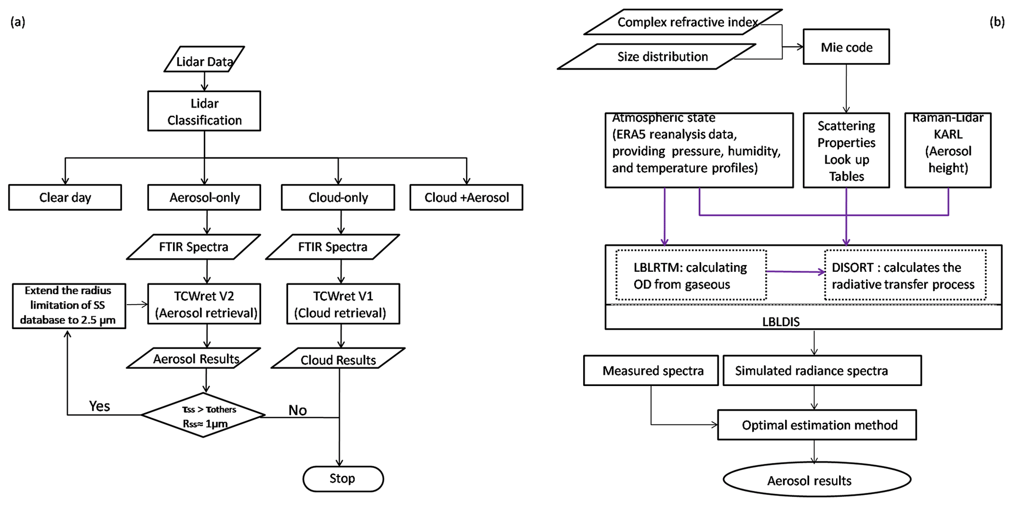
The aerosol or cloud height is determined from the KARL measurements and is provided to the TCWret retrieval algorithm (see Sect. 3.1). For cloud-only observations, the first version of the algorithm, TCWret V1, is used to retrieve cloud parameters, as described by Richter et al. (2022). For aerosol-only events, the modified version, TCWret V2, is used to carry out the aerosol components retrieval. For complex situations with the simultaneous existence of clouds and aerosols, the concurrent NYAEM-FTS measurements will be excluded. A flow diagram of the joint-observation scheme is found in Fig. 2a.
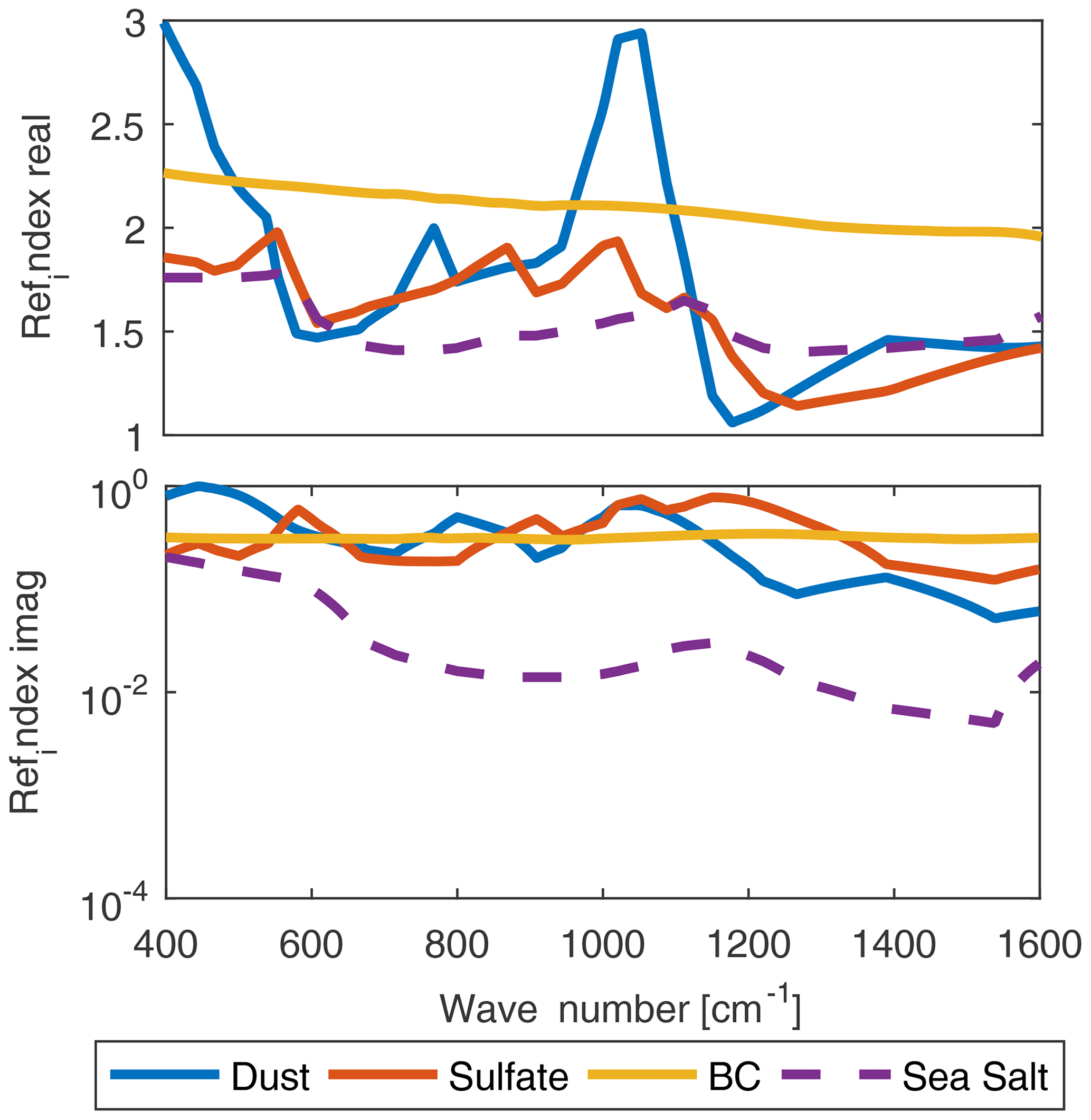
Figure 3The complex refractive index of dust, sulfate, BC, and sea salt. The complex imaginary refractive indices of sulfate and dust are based on the OPAC/GADA database, BC is from Chang and Charalampopoulos (1990), and sea salt is from Eldridge and Palik (1997) and Palik (1997).
A flow diagram of TCWret V2 is given in Fig. 2b. As shown in Fig. 2b, there are several inputs for model simulations. Firstly, scattering coefficient databases for different aerosol types are calculated using Mie code (Mishchenko et al., 1999) based on the aerosol complex refractive index and the aerosol size distribution. Secondly, the atmospheric state profile, which includes temperature, humidity, and pressure (referred to as THP), is obtained from ERA5 reanalysis data with a time resolution of 3 h (Hersbach et al., 2018). Thirdly, the aerosol height information, which is provided by the KARL (Sect. 2.3), is obtained as input. Finally, to obtain the temperature of the aerosol layer (the fourth input), the ERA5 temperature is interpolated to the altitude measured by the KARL. Furthermore, for all aerosol types, the a priori information of aerosol is fixed as an aerosol optical depth (AOD) of 0.0001 and an Reff of 0.35 µm.
3.1.3 Artificial spectra from LBLDIS
When considering downwelling emissions from the atmosphere on a clear day, the main contributions to emissions in the thermal infrared band are from greenhouse gases, i.e., CO2, H2O, N2O, CO, CH4, and O3. If there is a cloud or aerosol layer, its broadband emissions can also be observed (see Fig. 1).
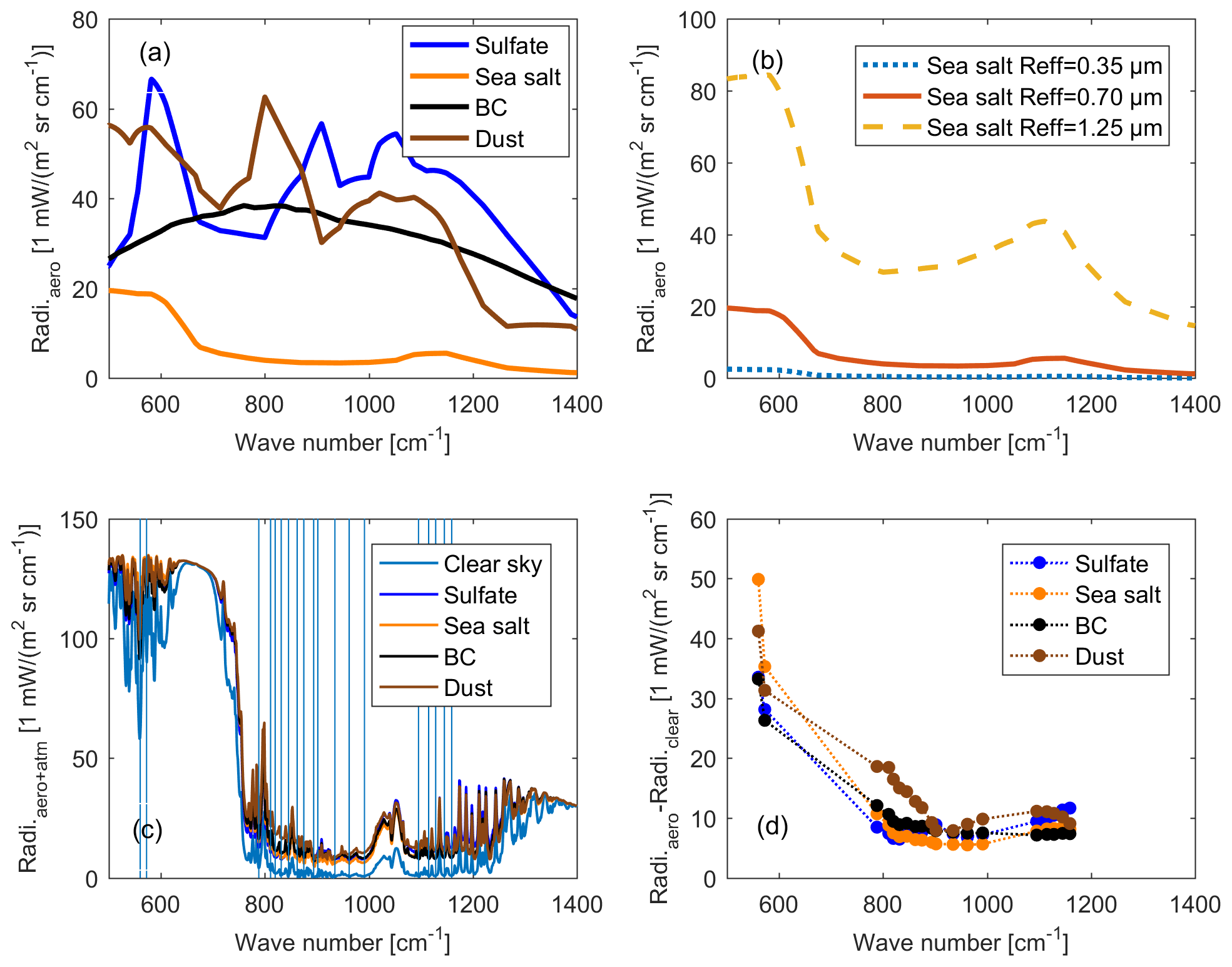
Figure 4(a) Emission spectra of small aerosol particles (dust – brown, sulfate – blue, sea salt – orange, and BC – black) with a Reff = 0.35 µm and a number density = 2000 cm−3; (b) emission spectra of sea salt with different particle sizes; (c) emission spectra of aerosols (AOD = 0.1) with atmospheric gases and for the clear-sky case; and (d) the difference between the total emission spectra of the aerosol and clear-sky cases in microwindows. The vertical blue lines in panel (c) show the middle values of the microwindows selected for retrieval. The emission spectra are simulated from LBLDIS with a resolution of 1 cm−1.
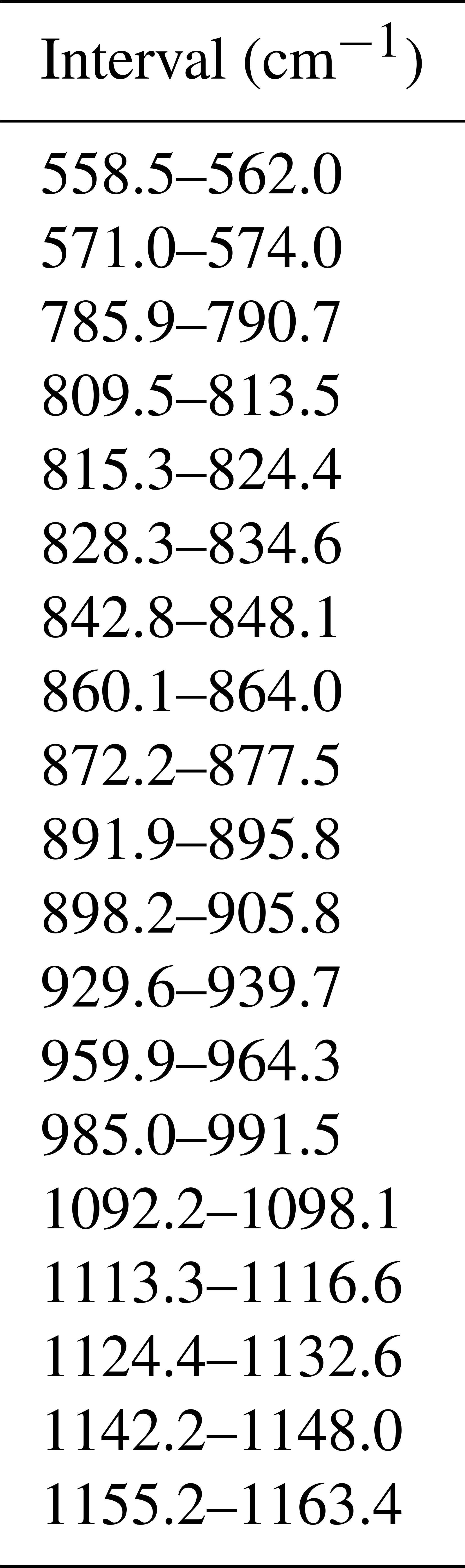
Several thermal infrared emission spectra from the LBLDIS model are shown in Fig. 4. Using the same number density, different aerosol types exhibit unique characteristics in the infrared emission spectra (shown in Fig. 4a). Among those aerosols, the radiance emitted from sea salt is lowest, due to its low light-absorbing capability compared with other aerosols. When the number density is fixed in model simulation, the radiance from sea salt increases with the size of particles (Fig. 4b). Other larger aerosol types are presented in Fig. A1. Using the same number density, the radiance from sea salt particles that are the same size as other aerosols is significantly lower; the radiances are only comparable when sea salt has a large particle size compared with the other aerosols. Figure 4c shows the thermal infrared emission spectra of atmospheric gases (clear sky) and different aerosols within atmosphere. According to Fig. 4c, the gas emissions dominate over the aerosol signal in some wave bands. Those bands are not considered for the retrieval, e.g., CO2 between 640 and 690 cm−1 and O3 between 1000 and 1100 cm−1. Aerosol windows (see Fig. A1) are chosen in the 500–600, 800–1000, and 1100–1200 cm−1 regions, which are selected as retrieval microwindows (vertical lines in Fig. 4c and compare Table A1). The spectra in Fig. 4d are shown in the form of the difference between the aerosol and clear-sky conditions in these microwindows. Based on this information, the emission spectra of aerosol events are different from one another; thus, the emissions from aerosols can be measured, and the aerosol types can be retrieved using the emission FTS. The reason for avoiding the gas emissions is the dependency of these emissions on the atmospheric temperature distribution.
3.1.4 Error estimation
In order to investigate the precision of the retrieved values, artificial spectra simulated from LBLDIS are used to explore the performance of TCWret V2 in the retrieval of aerosol types. Artificial spectra with preset AOD and Reff values are created using LBLDIS and then act as measured spectra retrieved by the algorithm. Specifically, we assume that all particles are concentrated at a single level: 2000 m a.g.l. (above ground level). The AOD values of sea salt, sulfate, dust, and BC are all set to 0.1, and the Reff is set to 0.7 µm. However, the retrieval results suffer from several uncertainty sources, as outlined in the following:
-
The aerosol height is a source of uncertainty, similar to the error in the aerosol layer temperature, as the aerosol height in this study is given by lidar measurement.
-
Uncertainty in the humidity profile has a significant signal with respect to the far-infrared emission spectrum, at about 1500–2000 cm−1; thus, the water vapor profile could change the radiance of the emission spectrum, which might affect the retrieval results.
-
Calibration uncertainty in the measured spectra is also an important source of uncertainty in the retrieval and could be caused by misreading the blackbody temperature. In this study, the total power calibration method (Revercomb et al., 1988) is used to calibrate the spectra. Assuming that the accuracy of the blackbody temperature is K, the propagation of this error into radiance is
According to Richter et al. (2022), the partial derivative can be estimated using
where B(Thot) is the hot blackbody temperature and B(Tamb) is the surface air temperature. With Thot=100 ∘C and Tamb=0 ∘C, = 0.41 mW sr−1 m−2 cm−1 is an average for the spectral interval between 500 and 2000 cm−1.
-
Measurement uncertainty is a source of uncertainty in the retrieval results, as the noise in the spectrum is assumed to be white in space and time.
-
Database uncertainty could be caused by uncertainty in the aerosol complex refractive index; both the real and imaginary part of the index could have an influence on the accuracy of the aerosol scattering property lookup tables, as mentioned in Sect. 3.1.1.
Table 2Parameter errors and modifications for artificial spectra.
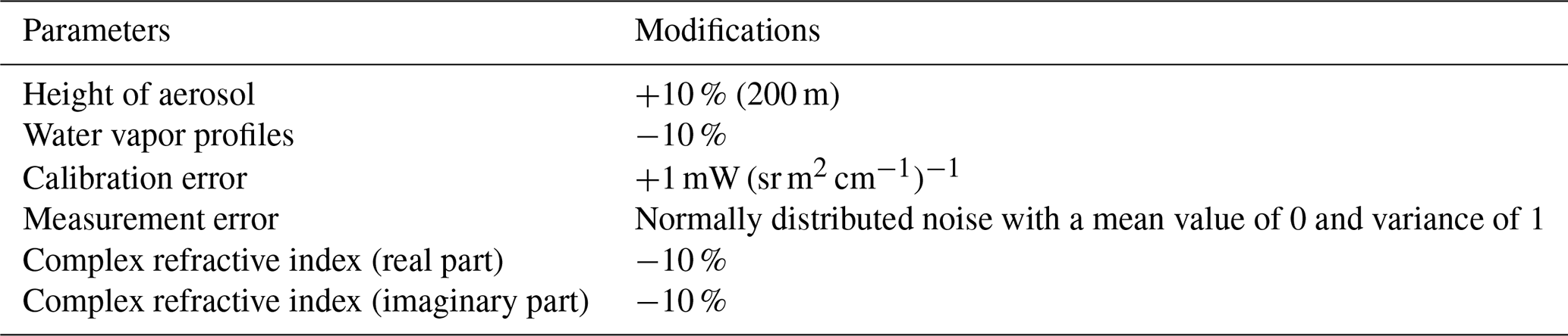
The artificial spectra with modifications are simulated according to Table 2. Compared with preset values, one can then compute the difference between retrieved values and preset values by perturbing each parameter.
3.2 AErosol RObotic NETwork (AERONET) and Modern-Era Retrospective analysis for Research and Applications version 2 (MERRA-2) AOD
The AERONET dataset provides aerosol products that are primarily in the visible wave band. Additionally, MERRA-2 provides aerosol information. Hence, it is worth investigating whether our measurements can be combined with existing data to provide more comprehensive aerosol information in the future. In this paper, we summarize the results from AERONET and MERRA-2 in the aerosol case in order to provide a general understanding of the aerosol events (see Fig. 8).
The AERONET project is a federation of ground-based remote sensing aerosol networks. It is widely used as a ground-based reference for the validation of aerosol retrievals. In Ny-Ålesund, a Sun photometer measuring solar extinction at several wavelengths is adopted to give the daily variance in AOD on 10 June 2020.
MERRA-2 is the latest version of the global atmospheric reanalysis dataset produced by the NASA Global Modeling and Assimilation Office (GMAO) using the Goddard Earth Observing System (GEOS, version 5.12.4) model. Hourly time-averaged two-dimensional data collection (M2T1NXAER) in MERRA-2 is used in this study (Gelaro et al., 2017). This collection consists of assimilated aerosol diagnostics, such as column mass density of aerosol components (BC, dust, sea salt, sulfate, and organic carbon), surface mass concentration of aerosol components, and the total extinction (and scattering) AOD at 550 nm. The dataset covers the period from 1980 to the present. In this paper, the AOD of sea salt, sulfate, dust, BC, and organic carbon in Ny-Ålesund are shown for 10 June 2020.
4.1 Artificial spectra retrieval
As we mentioned in Sect. 3.1.4, the artificial spectra are given by a forward model with preset values (see Table 2). The retrieved results of those artificial spectra can be obtained by using the artificial spectra as the observed spectra in the retrieval algorithm. The difference between retrieved values with the preset values and those obtained by perturbing each parameter is shown in Fig. 5.
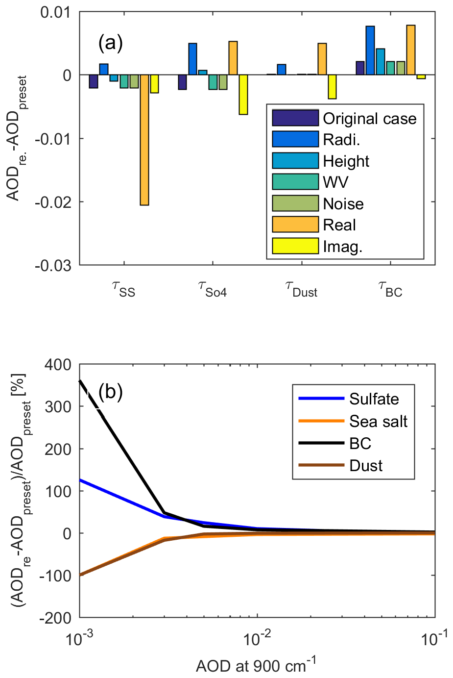
Figure 5(a) The difference between the retrieved AOD in the original case with preset values and that with several possible perturbations (see Table 2). (b) The relative uncertainties in the AOD in the original cases with several preset values. Note that the artificial spectra with several preset values in panel (b) mean that the AOD values of aerosols are set from 0.001 to 0.1. Using the same method but for different preset AOD values, the reliable range of AOD values is given in panel (b).
Figure 5a shows that the original case, without any modifications, is close to the preset values. The difference between the AOD retrieved in the original case and the preset values is less than 0.005 at 900 cm−1, leading to convincing results using this retrieval algorithm. Noise in the measurements and water vapor (WV) profiles have small effects on the retrieval. The most important parameter is the database error, caused by the uncertainty in the complex refractive index. A decrease of 10 % in the real part of the complex refractive index will cause a positive error of about 7 % in the AOD of sulfate, dust, and BC, although it causes negative error of 18 % in the AOD of sea salt. While a 10 % decrease in the imaginary part of the complex refractive index will cause a negative error of about 4 % in the AOD of sulfate, dust, and BC, it causes a negative error of 1 % in the AOD of sea salt. Following the database errors, the second most important error is the calibration error, e.g., a 1 K error in the blackbody temperature will cause a change in radiance of about 0.47 mW sr−1 m−2 cm−1. An offset of radiance by 1 mW sr−1 m−2 cm−1 causes an approximate 4 % overestimation in the results. The temperature error in the aerosol layer is the third most important effect in the aerosol retrieval.
In order to show the reliable range of the retrieved AOD, using similar artificial spectra but for several AOD from 0.001 to 0.1 at 900 cm−1, the relative uncertainties in the AOD original case with preset values are given in Fig. 5b. The uncertainty in the AOD retrieval is 0.0015; hence, aerosols are reliably retrieved when the AOD is > 0.003. Therefore, we consider the results to be reliable when the retrieved AOD is greater than 0.003.
Organic carbon (OC) is one of the major components in tropospheric aerosols. However, it is not considered because no complex refractive index data exist in the infrared wave band of OC. There are also many types of OC, and each of them has a different spectral signature. We assume that the spectral signature of OC is very weak. However, if there are spectral features which are not fitted, e.g., due to the presence of aerosol types that are not accounted for in the scattering database, the error margin on the retrieved aerosol types will be increased.
In conclusion, when aerosol is present in the atmosphere, the emission from aerosol can be measured by FTS. According to forward-model simulations, different aerosol types show their own features. Using artificial spectra with preset values, error estimations caused by the retrieval could be calculated.
4.2 Aerosol-only retrieval
On 10 June 2020, there was a distinct aerosol event in Ny-Ålesund (see the aerosol distribution derived using the KARL in Fig. 6). This aerosol event is chosen as our aerosol-only case. Figure 7 presents the four different aerosol classes and cloud based on the lidar classification method (see Sect. 2.3). During this day, aerosols were mainly distributed below 1500 m (see Fig. 6). From 07:00 to 11:00 UTC, the thickness of a coarse aerosol layer (dense aerosol according to the lidar classification method in Sect. 2.3) near the surface decreased, while this aerosol load increased and split into two layers, one layer near the surface and another activated aerosol layer (at a height of about 500 m), in the afternoon. At around 08:00 UTC, clouds were present at a height of 3500 m; this was screened out in the aerosol-only FTS retrieval.
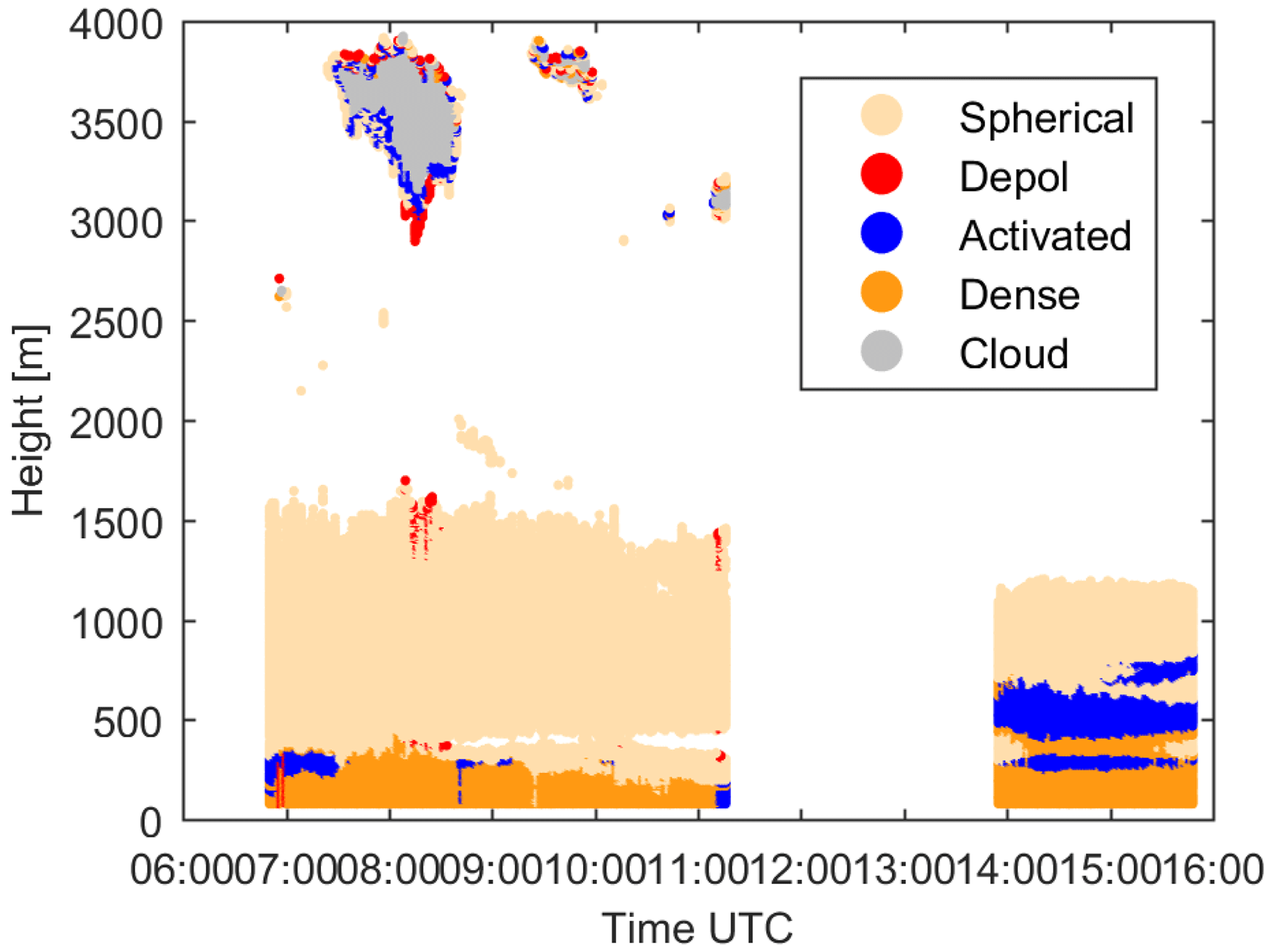
Figure 6Four different aerosol classes (spherical particles – light yellow, depolarization particles – red, activated particles – blue, and dense particles – dark yellow) and cloud (gray) on 10 June 2020 based on the lidar classification method.
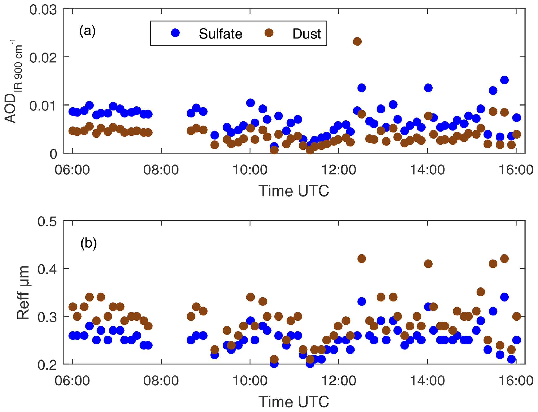
Figure 7(a) The AOD of sulfate (blue) and dust (brown) retrieved from emission FTS measurements and (b) Reff results with same color information on 10 June 2020.
Figure 7 shows the results retrieved from the FTS. From Fig. 7a, it can be seen that the dominant aerosol above Ny-Ålesund is sulfate (a daily average of about AOD = 0.007 ± 0.0027). Dust also exists but generally at lower concentrations than sulfate (daily average of about AOD = 0.0039 ± 0.0029). The AOD values of BC and sea salt are much lower than the reliable range of AOD; therefore, the retrieved values of BC and sea salt are not presented. From 09:00 to 11:00 UTC, the AOD of sulfate decreases with time; after that, it increases slowly from 12:00 to 14:00 UTC (before reaching approximately 0.0135 at 14:00 UTC). With respect to daily variation, dust (as the second most dominant aerosol) does not show daily variation that is as significant as that of sulfate. From the long-term observations, it is found that dust and sulfate are independent in the retrieval (see Fig. 9), which will be discussed in the following section. Considering the uncertainty in the dust retrieval and the reliable range of the retrieval, it can be concluded that the AOD of dust is relatively stable during the aforementioned day. From Fig. 7b, it can be seen that both sulfate and dust are small in size (0.25 ± 0.03 and 0.30 ± 0.06 µm, respectively).
Figure 8 shows the AOD from the FTS, AERONET, and MERRA-2. In this analysis, the AOD from the FTS will be called AODIR, the AOD from AERONET will be referred to as AODAERO, and the AOD from MERRA-2 will be written as AODMERRA-2. From the Sun photometer (AERONET) measurements, as shown in Fig. 8a, the AODAERO (blue line for 500 nm and red line for 780 nm) decreases from 08:00 to 11:00 UTC and increases after 14:24 UTC. Compared with AERONET, AODIR (black line) shows similar daily variation, whereas the minimum in AODMERRA-2 (orange line) is at 08:00 UTC, about 3 h earlier than AODIR and AODAERO. According to MERRA-2 reanalysis data, as shown in Fig. 8b, the first two major aerosol components are sulfate and dust, which is consistent with AODIR in Fig. 8. Furthermore, the daily variation in AODMERRA-2 on 10 June 2020 is mainly caused by sulfate and sea salt. Apart from sea salt, which shows a limited signal in the infrared wave band, the daily variation in sulfate in MERRA-2 is also similar to the FTS measurement, but the turning point in MERRA-2 is about 3 h earlier than that in the observations. In conclusion, the agreement in the daily variation between the FTS measurements and the Sun photometer measurements as well as the consistency in the dominant aerosol components between the FTS and MERRA-2 reanalysis data support the high quality of the FTS retrieval results.
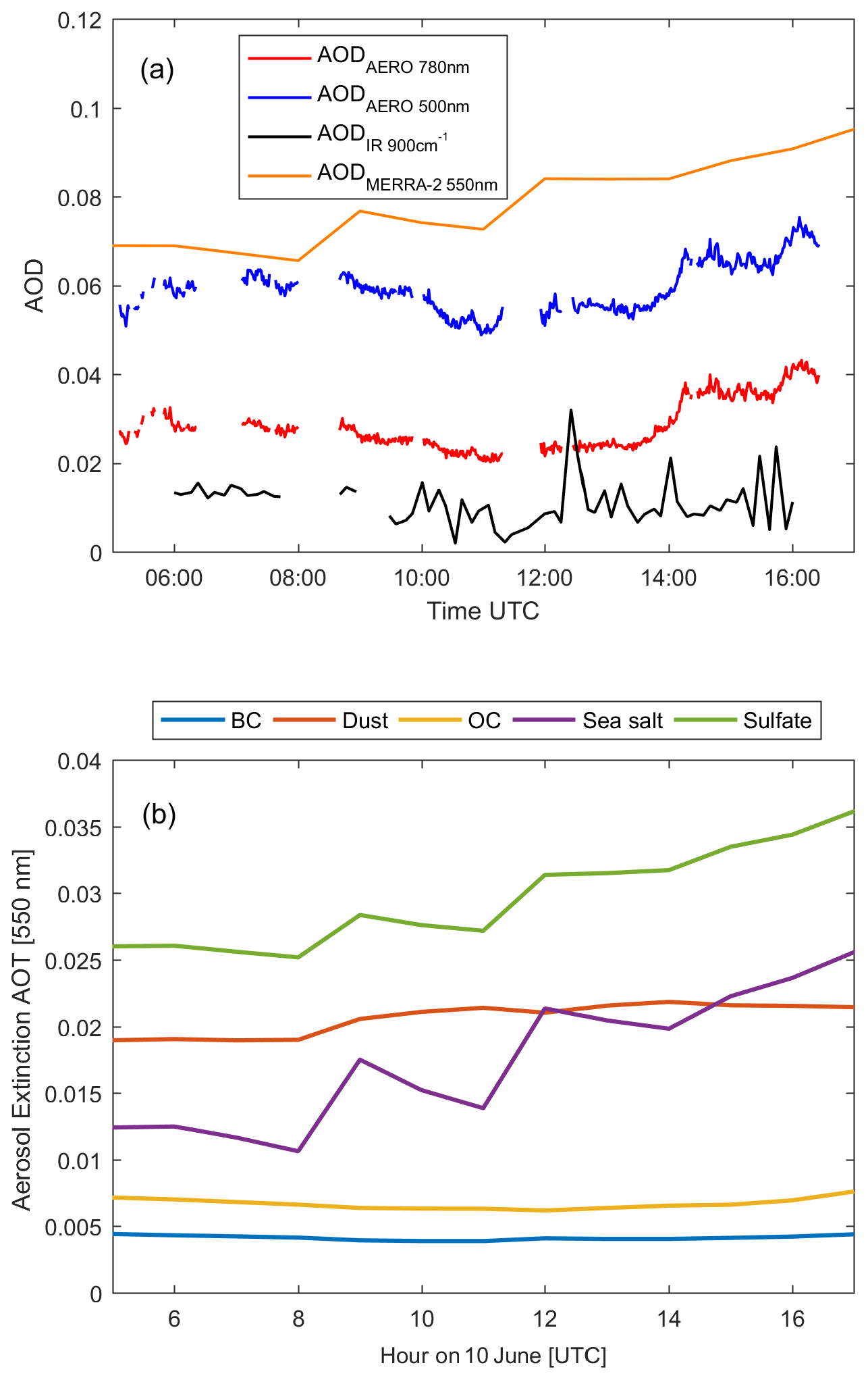
Figure 8(a) AOD measured by a Sun photometer (AERONET, 500 nm in blue and 780 nm in red), AOD measured by the FTS (900 cm−1 in black), and AOD from MERRA-2 reanalysis data (550 nm) in Ny-Ålesund on 10 June 2020. (b) The AOD of different aerosol components in MERRA-2 reanalysis data in Ny-Ålesund on 10 June 2020. AERONET data are from https://www.mdpi.com/2072-4292/11/11/1362 (last access: 6 December 2022), and MERRA-2 data are from https://goldsmr4.gesdisc.eosdis.nasa.gov/data/MERRA2/M2T1NXAER.5.12.4/ (last access: 6 December 2022).
Additionally, according to the lidar measurements (see Fig. 6), there are indications of activated aerosol at a height of about 500 m in the afternoon. In the FTS retrieval algorithm, the aerosol databases do not include liquid water nor activated particles; thus, only dry particles are considered in our retrieval. The appearance of an activated aerosol signal indicates that hygroscopic growth of aerosol needs to be considered in the aerosol scattering property lookup tables, which will be the focus of future research.
4.3 Long-term observation
For the continuous long-term observation of aerosols, Cloudnet (Illingworth et al., 2007) is a better alternative than the KARL measurements due to its improved data continuity as well as the inclusion of aerosol height data and cloud-type information. With the Cloudnet dataset, aerosol-only situations can be distinguished, and the corresponding spectra are retrieved using TCWret V2. The results are presented in Fig. 9. The dominant aerosol type varies from April to August and is not fixed. For sulfate is often present in the Arctic, although it is higher during springtime and lower in summer. Similarly, BC is also frequently observed in the Arctic, with less obvious seasonal variation than sulfate. A BC outburst event is observed each spring and summer. In spring, sulfate and BC concentrations are significant, whereas sea salt and dust concentrations are lower. In addition, a sea salt enhancement event is observed in summer, possibly due to emissions from nearby open water. Figure 9b, c, d, e, f, and g present correlation plots between different aerosol types. None of these plots show a clear correlation; thus, the species in question can be retrieved independently of one another.
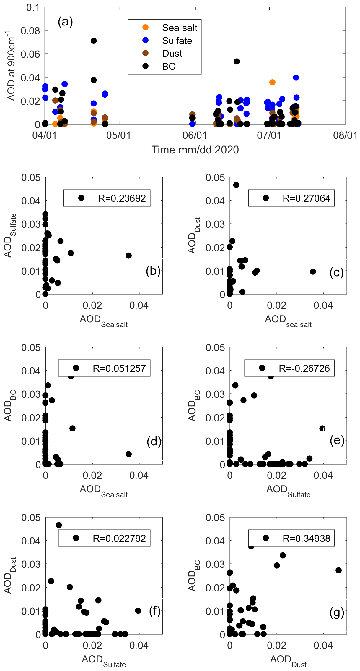
Figure 9(a) Long-term observations using FTS (from April to August). The correlations between (b) sea salt and sulfate, (c) sea salt and dust, (d) sea salt and BC, (e) sulfate and BC, (f) sulfate and dust, and (g) dust and BC.
The FTS instrument, NYAEM-FTS, which is used to measure downwelling emitted radiation, has been in operation since 2019. Using the NYAEM-FTS in combination with the KARL, aerosols can be observed more comprehensively than by either instrument alone.
For the FTS emission measurements, according to forward-model simulation, the aerosol signatures of different aerosol types in the infrared spectral region are quite clear and independent. The TCWret V1 retrieval algorithm (Richter et al., 2022) has been modified for retrieval of the optical depth and Reff of different aerosol types. Combining lidar and FTS, a two-instrument joint-measurement scheme has been designed and applied to carry out aerosol component retrieval. The measurements from both instruments are analyzed using a case study on 10 June 2020 (aerosol-only case) to show the potential synergy.
In the aerosol-only case study on 10 June 2020, the cloud and aerosol signals could be clearly distinguished using measurements from the KARL. From the emission FTS measurements, we see that sulfate is the dominant aerosol throughout the day. Compared with Sun photometer measurements, the daily variation in the aerosol AOD is mainly affected by sulfate in the infrared. Comparing the results from the NYAEM-FTS with MERRA-2 reanalysis data, the proportions of sulfate, dust, and BC show good agreement.
For long-term observations from April to August 2020, it can be seen that sulfate is often present in the Arctic, although it is higher during springtime and relatively lower in summer. Similarly, BC is also frequently observed in the Arctic, with less obvious seasonal variation compared with sulfate. During the springtime, sulfate and BC concentrations are significant, whereas sea salt and dust abundances are relatively low. None of these species show a clear correlation with one another; thus, they can be retrieved independently.
The database used in TCWret V2 does not include activated particles, which will be the subject of a future study.
The retrieval method adopted in the modified TCWret algorithm for the aerosol case is an optimal estimation method (Rodgers, 2000), and the relationship between a measured emission spectrum y and the unknown aerosol state x can be described by a simple mathematical model:
where F(x) is the forward model and ε is the error in observation. The solution of the inverse problem is the state x minimizing a cost function ξ2(x) usually defined as
where is the inverse measurement error covariance matrix, containing the variances of the spectral radiance; xa is the a priori; and is the inverse error in the a priori covariance matrix xa. The state vector x in the modified TCWret algorithm is defined as follows: , where τ is the AOD of aerosols and r is the Reff of aerosols.
As the forward model is a nonlinear function, an iterative method is needed to minimize the cost function ξ2(x):
Here xn and xn+1 are the aerosol parameters of the nth and (n+1)th step, and sn is the modification of the aerosol parameters during the nth iteration. For weak nonlinear problems, the Gauss–Newton (GN) method can be successfully applied. In significant nonlinear situations, however, the GN method is not guaranteed to decrease the cost function; therefore, the method of steepest descent could be used. The Levenberg–Marquardt (LM) method modification combines both methods by starting with the steepest descent method far away from the minimum and using the GN method near the minimum. At each iteration, a damping factor μ is adjusted in such a way that if the step results in a decrease in the cost function, the damping factor μ is decreased, bringing the next step closer to the GN step. If the step causes the cost function to increase, the iteration is repeated with a higher damping factor μ, resulting in a step closer to the gradient descent direction (Ceccherini and Ridolfi, 2010). The adjustment vector sn could be determined by the following governing equation:
where is the Jacobian matrix; i denotes the parameters in the state vector; is the inverse measurement error covariance matrix, containing the variances of the spectral radiance; xa is the a priori; is the inverse error of the a priori covariance matrix xa; is the LM term, as previously mentioned; F(xi) is the calculated spectral radiance; and y is the measured spectral radiance.
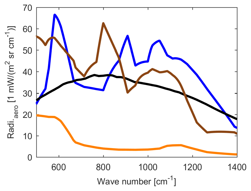
Figure A1The emission spectra of large aerosol particles (dust – brown, sulfate – blue, sea salt – orange, and BC – black) with a Reff = 0.70 µm and a number density = 2000 cm−3.
The iteration is said to have converged if the cost function ξ2 does not change anymore, i.e., the change in the cost function ξ is below a threshold. This threshold is set 0.001 in this study, i.e., the iteration has converged if
Averaging kernels
The averaging kernels are a useful diagnostic tool to characterize the solution of the retrieval. In TCWret, averaging kernels are calculated as follows:
where xr is the retrieved state vector, x is the true value of the state vector, Tr is the final transfer matrix T, and Kr is the final Jacobian matrix. According to Ceccherini and Ridolfi (2010), the final transfer matrix could be calculated as follows:
where 0 is a zero matrix and I is an identity matrix; the other quantities have been described above. The matrices Kn are calculated in Eq. (A4). The calculation of the transfer matrix is performed in parallel to the minimization. The following is an example of averaging kernels:
The averaging kernels belong to the retrieved result, as they include a lot of information about the retrieval results, e.g., how much influence is exerted by the a priori and how independent the retrieved quantities are from one another. On the diagonal elements, one finds the derivatives of each element in the retrieved state vector with respect to its corresponding element in the true state vector. From the averaging kernel, the AOD of sulfate is the parameter least dependent on a priori information, followed by the AOD of dust and sea salt. Except for dust, all other aerosol size information is difficult to retrieve. Moreover, the information in each row or column suggests that there is very little connection between the parameters and that they are all independent of one another, supporting the finding of a low correlation in Sect. 4.3.
Table A1Microwindows used in TCWret to retrieve the microphysical aerosol or cloud parameters (Richter et al., 2022).
The latest version of TCWret can be downloaded from Zenodo (https://doi.org/10.5281/zenodo.3948048, Richter et al., 2022). The lidar data, spectra measured from the emission FTS, and retrieval results are available from the corresponding author upon request. AERONET data are from https://www.mdpi.com/2072-4292/11/11/1362 (last access: 6 December 2022; Graßl and Ritter, 2019). MERRA-2 data are from https://goldsmr4.gesdisc.eosdis.nasa.gov/data/MERRA2/M2T1NXAER.5.12.4/ (last access: 6 December 2022; Gelaro et al., 2017).
PR implemented TCWret V1 and DJ developed it into TCWret V2, the retrieval of aerosol parameters. MP designed and built the measurement setup, performed measurements, and gave advice on the development of TCWret. CR performed lidar measurements and gave advice on using the lidar and Sun photometer data. XS gave advice on forward-model simulation. MB gave advice on the calibration processes, performed the measurements, and maintained the instrument. JN gave advice on the measurement setup and the development of TCWret. All authors contributed to the paper.
At least one of the (co-)authors is a member of the editorial board of Atmospheric Measurement Techniques. The peer-review process was guided by an independent editor, and the authors also have no other competing interests to declare.
Publisher's note: Copernicus Publications remains neutral with regard to jurisdictional claims in published maps and institutional affiliations.
We gratefully acknowledge funding from the Deutsche Forschungsgemeinschaft (DFG, German Research Foundation) within the framework of the Transregional Collaborative Research Center “TRR 172: ArctiC Amplification: Climate Relevant Atmospheric and SurfaCe Processes, and Feedback Mechanisms (AC)3” program “E02: Ny-Ålesund Column Thermodynamic Structure, Clouds, Aerosols, Trace Gases and Radiative Effects” subproject (project no. 268020496). We thank the AWI Bremerhaven and the AWI Potsdam for logistical support at the AWIPEV research base and the station personnel for on-site support. We thank the senate of Bremen for partial funding of this work.
This research has been supported by the University of Bremen and the German Research Foundation (DFG, grant no. 268020496-TRR 172-(AC)3).
The article processing charges for this open-access publication were covered by the University of Bremen.
This paper was edited by Alexander Kokhanovsky and reviewed by three anonymous referees.
Abbatt, J. P. D., Leaitch, W. R., Aliabadi, A. A., Bertram, A. K., Blanchet, J.-P., Boivin-Rioux, A., Bozem, H., Burkart, J., Chang, R. Y. W., Charette, J., Chaubey, J. P., Christensen, R. J., Cirisan, A., Collins, D. B., Croft, B., Dionne, J., Evans, G. J., Fletcher, C. G., Galí, M., Ghahreman, R., Girard, E., Gong, W., Gosselin, M., Gourdal, M., Hanna, S. J., Hayashida, H., Herber, A. B., Hesaraki, S., Hoor, P., Huang, L., Hussherr, R., Irish, V. E., Keita, S. A., Kodros, J. K., Köllner, F., Kolonjari, F., Kunkel, D., Ladino, L. A., Law, K., Levasseur, M., Libois, Q., Liggio, J., Lizotte, M., Macdonald, K. M., Mahmood, R., Martin, R. V., Mason, R. H., Miller, L. A., Moravek, A., Mortenson, E., Mungall, E. L., Murphy, J. G., Namazi, M., Norman, A.-L., O'Neill, N. T., Pierce, J. R., Russell, L. M., Schneider, J., Schulz, H., Sharma, S., Si, M., Staebler, R. M., Steiner, N. S., Thomas, J. L., von Salzen, K., Wentzell, J. J. B., Willis, M. D., Wentworth, G. R., Xu, J.-W., and Yakobi-Hancock, J. D.: Overview paper: New insights into aerosol and climate in the Arctic, Atmos. Chem. Phys., 19, 2527–2560, https://doi.org/10.5194/acp-19-2527-2019, 2019. a
Asmi, E., Kondratyev, V., Brus, D., Laurila, T., Lihavainen, H., Backman, J., Vakkari, V., Aurela, M., Hatakka, J., Viisanen, Y., Uttal, T., Ivakhov, V., and Makshtas, A.: Aerosol size distribution seasonal characteristics measured in Tiksi, Russian Arctic, Atmos. Chem. Phys., 16, 1271–1287, https://doi.org/10.5194/acp-16-1271-2016, 2016. a
Bond, T. C.,d Doherty, S. J., Fahey, D. W., Forster, P. M., Berntsen, T., DeAngelo, B. J., Flanner, M. G., Ghan, S., Kärcher, B., Koch, D., Kinne, S., Kondo, Y., Quinn, P. K., Sarofim, M. C., Schultz, M. G., Schulz, M., Venkataraman, C., Zhang, H., Zhang, S., Bellouin, N., Guttikunda, S. K., Hopke, P. K., Jacobson, M. Z., Kaiser, J. W., Klimont, Z., Lohmann, U., Schwarz, J. P., Shindell, D., Storelvmo, T., Warren, S. G., and Zender, C. S.: Bounding the role of black carbon in the climate system: A scientific assessment, J. Geophys. Res.-Atmos., 118, 5380–5552, https://doi.org/10.1002/jgrd.50171, 2013. a
Bony, S., Colman, R., Kattsov, V. M., Allan, R. P., Bretherton, C. S., Dufresne, J.-L., Hall, A., Hallegatte, S., Holland, M. M., Ingram, W., Randall, D. A., Soden, B. J., Tselioudis, G., and Webb, M. J.: How Well Do We Understand and Evaluate Climate Change Feedback Processes?, J. Climate, 19, 3445–3482, https://doi.org/10.1175/JCLI3819.1, 2006. a
Boyer, M., Aliaga, D., Pernov, J. B., Angot, H., Quéléver, L. L. J., Dada, L., Heutte, B., Dall'Osto, M., Beddows, D. C. S., Brasseur, Z., Beck, I., Bucci, S., Duetsch, M., Stohl, A., Laurila, T., Asmi, E., Massling, A., Thomas, D. C., Nøjgaard, J. K., Chan, T., Sharma, S., Tunved, P., Krejci, R., Hansson, H. C., Bianchi, F., Lehtipalo, K., Wiedensohler, A., Weinhold, K., Kulmala, M., Petäjä, T., Sipilä, M., Schmale, J., and Jokinen, T.: A full year of aerosol size distribution data from the central Arctic under an extreme positive Arctic Oscillation: insights from the Multidisciplinary drifting Observatory for the Study of Arctic Climate (MOSAiC) expedition, Atmos. Chem. Phys., 23, 389–415, https://doi.org/10.5194/acp-23-389-2023, 2023. a
Ceccherini, S. and Ridolfi, M.: Technical Note: Variance-covariance matrix and averaging kernels for the Levenberg-Marquardt solution of the retrieval of atmospheric vertical profiles, Atmos. Chem. Phys., 10, 3131–3139, https://doi.org/10.5194/acp-10-3131-2010, 2010. a, b
Chang, H.-C. and Charalampopoulos, T.: Determination of the wavelength dependence of refractive indices of flame soot, Proc. R. Soc. London, Ser. A, 430, 577–591, https://doi.org/10.1098/rspa.1990.0107, 1990. a, b
Clough, S., Shephard, M., Mlawer, E., Delamere, J., Iacono, M., Cady-Pereira, K., Boukabara, S., and Brown, P.: Atmospheric radiative transfer modeling: a summary of the AER codes, J. Quant. Spectrosc. Ra., 91, 233–244, https://doi.org/10.1016/j.jqsrt.2004.05.058, 2005. a
Domine, F., Sparapani, R., Ianniello, A., and Beine, H. J.: The origin of sea salt in snow on Arctic sea ice and in coastal regions, Atmos. Chem. Phys., 4, 2259–2271, https://doi.org/10.5194/acp-4-2259-2004, 2004. a
Donth, T., Jäkel, E., Ehrlich, A., Heinold, B., Schacht, J., Herber, A., Zanatta, M., and Wendisch, M.: Combining atmospheric and snow radiative transfer models to assess the solar radiative effects of black carbon in the Arctic, Atmos. Chem. Phys., 20, 8139–8156, https://doi.org/10.5194/acp-20-8139-2020, 2020. a
Eldridge, J. and Palik, E. D.: Sodium Chloride (NaCl), in: Handbook of Optical Constants of Solids, edited by: Palik, E. D., Academic Press, Burlington, 775–793, https://doi.org/10.1016/B978-012544415-6.50041-8, 1997. a, b
Fan, J., Wang, Y., Rosenfeld, D., and Liu, X.: Review of Aerosol–Cloud Interactions: Mechanisms, Significance, and Challenges, J. Atmos. Sci., 73, 4221–4252, https://doi.org/10.1175/JAS-D-16-0037.1, 2016. a
Francis, D., Eayrs, C., Chaboureau, J.-P., Mote, T., and Holland, D. M.: Polar jet associated circulation triggered a Saharan cyclone and derived the poleward transport of the African dust generated by the cyclone, J. Geophys. Res.-Atmos., 123, 11–899, https://doi.org/10.1029/2018JD029095, 2018. a
Francis, D., Eayrs, C., Chaboureau, J.-P., Mote, T., and Holland, D. M.: A meandering polar jet caused the development of a Saharan cyclone and the transport of dust toward Greenland, Adv. Sci. Res., 16, 49–56, https://doi.org/10.5194/asr-16-49-2019, 2019. a
Freudenthaler, V., Esselborn, M., Wiegner, M., Heese, B., Tesche, M., Ansmann, A., Müller, D., Althausen, D., Wirth, M., Fix, A., Ehret, G., Knippertz, P., Toledano, C., Gasteiger, J., Garhammer, M., and Seefeldner, M.: Depolarization ratio profiling at several wavelengths in pure Saharan dust during SAMUM 2006, Tellus B, 61, 165–179, https://doi.org/10.1111/j.1600-0889.2008.00396.x, 2009. a, b
Gelaro, R., McCarty, W., Suárez, M. J., Todling, R., Molod, A., Takacs, L., Randles, C. A., Darmenov, A., Bosilovich, M. G., Reichle, R., Wargan, K., Coy, L., Cullather, R., Draper, C., Akella, S., Buchard, V., Conaty, A., da Silva, A. M., Gu, W., Kim, G.-K., Koster, R., Lucchesi, R., Merkova, D., Nielsen, J. E., Partyka, G., Pawson, S., Putman, W., Rienecker, M., Schubert, S. D., Sienkiewicz, M., and Zhao, B.: The Modern-Era Retrospective Analysis for Research and Applications, Version 2 (MERRA-2), J. Climate, 30, 5419–5454, https://doi.org/10.1175/JCLI-D-16-0758.1, 2017 (data available at: https://goldsmr4.gesdisc.eosdis.nasa.gov/data/MERRA2/M2T1NXAER.5.12.4/, last access: 6 December 2022). a, b
Graßl, S. and Ritter, C.: Properties of Arctic Aerosol Based on Sun Photometer Long-Term Measurements in Ny-Ålesund, Svalbard, Remote Sens., 11, 1362, https://doi.org/10.3390/rs11111362, 2019. a
Graversen, R. G., Langen, P. L., and Mauritsen, T.: Polar Amplification in CCSM4: Contributions from the Lapse Rate and Surface Albedo Feedbacks, J. Climate, 27, 4433–4450, https://doi.org/10.1175/JCLI-D-13-00551.1, 2014. a
Hersbach, H., Bell, B., Berrisford, P., Biavati, G., Horányi, A., Muñoz Sabater, J., Nicolas, J., Peubey, C., Radu, R., Rozum, I., Schepers, D., Simmons, A., Soci, C., Dee, D., and Thépaut, J.-N.: ERA5 hourly data on pressure levels from 1979 to present, Copernicus climate change service (C3S) climate data store (CDS) [data set], https://doi.org/10.24381/cds.bd0915c6, 2018. a
Illingworth, A. J., Hogan, R. J., E., O., Bouniol, D., Brooks, M. E., Delanoé, J., Donovan, D. P., Eastment, J. D., Gaussiat, N., Goddard, J. W. F., Haeffelin, M., Baltink, H. K., Krasnov, O. A., Pelon, J., Piriou, J.-M., Protat, A., Russchenberg, H. W. J., Seifert, A., Tompkins, A. M., van Zadelhoff, G.-J., Vinit, F., Willén, U., Wilson, D. R., and Wrench, C. L.: Cloudnet: Continuous Evaluation of Cloud Profiles in Seven Operational Models Using Ground-Based Observations, B. Am. Meteorol. Soc., 88, 883–898, 2007. a
Koch, D., Bauer, S. E., Genio, A. D., Faluvegi, G., McConnell, J. R., Menon, S., Miller, R. L., Rind, D., Ruedy, R., Schmidt, G. A., and Shindell, D.: Coupled Aerosol-Chemistry–Climate Twentieth-Century Transient Model Investigation: Trends in Short-Lived Species and Climate Responses, J. Climate, 24, 2693–2714, https://doi.org/10.1175/2011JCLI3582.1, 2011. a
Kodros, J. K., Hanna, S. J., Bertram, A. K., Leaitch, W. R., Schulz, H., Herber, A. B., Zanatta, M., Burkart, J., Willis, M. D., Abbatt, J. P. D., and Pierce, J. R.: Size-resolved mixing state of black carbon in the Canadian high Arctic and implications for simulated direct radiative effect, Atmos. Chem. Phys., 18, 11345–11361, https://doi.org/10.5194/acp-18-11345-2018, 2018. a
Krinner, G., Boucher, O., and Balkanski, Y.: Ice-free glacial northern Asia due to dust deposition on snow, Clim. Dynam., 27, 613–625, https://doi.org/10.1007/s00382-006-0159-z, 2006. a
Lee, S.-M., Shi, H., Sohn, B.-J., Gasiewski, A. J., Meier, W. N., and Dybkjær, G.: Winter Snow Depth on Arctic Sea Ice From Satellite Radiometer Measurements (2003–2020): Regional Patterns and Trends, Geophys. Res. Lett., 48, e2021GL094541, https://doi.org/10.1029/2021GL094541, 2021. a
May, N., Quinn, P., McNamara, S., and Pratt, K.: Multiyear study of the dependence of sea salt aerosol on wind speed and sea ice conditions in the coastal Arctic, J. Geophys. Res.-Atmos., 121, 9208–9219, https://doi.org/10.1002/2016JD025273, 2016. a
Ming, J., Xiao, C., Cachier, H., Qin, D., Qin, X., Li, Z., and Pu, J.: Black Carbon (BC) in the snow of glaciers in west China and its potential effects on albedos, Atmos. Res., 92, 114–123, https://doi.org/10.1016/j.atmosres.2008.09.007, 2009. a
Mishchenko, M. I., Dlugach, J. M., Yanovitskij, E. G., and Zakharova, N. T.: Bidirectional reflectance of flat, optically thick particulate layers: an efficient radiative transfer solution and applications to snow and soil surfaces, J. Quant. Spectrosc. Ra., 63, 409–432, https://doi.org/10.1016/S0022-4073(99)00028-X, 1999. a, b, c
Palik, E. D.: Gallium Arsenide (GaAs), in: Handbook of Optical Constants of Solids, edited by: Palik, E. D., Academic Press, Burlington, 429–443, https://doi.org/10.1016/B978-012544415-6.50018-2, 1997. a, b
Park, J., Dall'Osto, M., Park, K., Gim, Y., Kang, H. J., Jang, E., Park, K.-T., Park, M., Yum, S. S., Jung, J., Lee, B. Y., and Yoon, Y. J.: Shipborne observations reveal contrasting Arctic marine, Arctic terrestrial and Pacific marine aerosol properties, Atmos. Chem. Phys., 20, 5573–5590, https://doi.org/10.5194/acp-20-5573-2020, 2020. a
Philipp, D., Stengel, M., and Ahrens, B.: Analyzing the Arctic Feedback Mechanism between Sea Ice and Low-Level Clouds Using 34 Years of Satellite Observations, J. Climate, 33, 7479–7501, https://doi.org/10.1175/JCLI-D-19-0895.1, 2020. a
Previdi, M., Smith, K. L., and Polvani, L. M.: Arctic amplification of climate change: a review of underlying mechanisms, Environ. Res. Lett., 16, 093003, https://doi.org/10.1088/1748-9326/ac1c29, 2021. a
Rathke, C. and Fischer, J.: Retrieval of Cloud Microphysical Properties from Thermal Infrared Observations by a Fast Iterative Radiance Fitting Method, J. Atmos. Ocean. Tech., 17, 1509–1524, https://doi.org/10.1175/1520-0426(2000)017<1509:ROCMPF>2.0.CO;2, 2000. a
Rathke, C., Notholt, J., Fischer, J., and Herber, A.: Properties of coastal Antarctic aerosol from combined FTIR spectrometer and sun photometer measurements, Geophys. Res. Lett., 29, 46-1–46-4, https://doi.org/10.1029/2002GL015395, 2002. a, b
Ren, L., Yang, Y., Wang, H., Zhang, R., Wang, P., and Liao, H.: Source attribution of Arctic black carbon and sulfate aerosols and associated Arctic surface warming during 1980–2018, Atmos. Chem. Phys., 20, 9067–9085, https://doi.org/10.5194/acp-20-9067-2020, 2020. a
Revercomb, H. E., Buijs, H., Howell, H. B., LaPorte, D. D., Smith, W. L., and Sromovsky, L. A.: Radiometric calibration of IR Fourier transform spectrometers: solution to a problem with the High-Resolution Interferometer Sounder, Appl. Optics, 27, 3210–3218, https://doi.org/10.1364/AO.27.003210, 1988. a, b
Richter, P.: RichterIUP/TCWret: Total Cloud Water retrieval (v1.0), Zenodo [code], https://doi.org/10.5281/zenodo.3948048, 2020. a
Richter, P., Palm, M., Weinzierl, C., Griesche, H., Rowe, P. M., and Notholt, J.: A dataset of microphysical cloud parameters, retrieved from Fourier-transform infrared (FTIR) emission spectra measured in Arctic summer 2017, Earth Syst. Sci. Data, 14, 2767–2784, https://doi.org/10.5194/essd-14-2767-2022, 2022. a, b, c, d, e, f, g, h
Ritter, C., Neuber, R., Schulz, A., Markowicz, K., Stachlewska, I., Lisok, J., Makuch, P., Pakszys, P., Markuszewski, P., Rozwadowska, A., Petelski, T., Zielinski, T., Becagli, S., Traversi, R., Udisti, R., and Gausa, M.: 2014 iAREA campaign on aerosol in Spitsbergen – Part 2: Optical properties from Raman-lidar and in situ observations at Ny-Ålesund, Atmos. Environ., 141, 1–19, https://doi.org/10.1016/j.atmosenv.2016.05.053, 2016. a, b, c, d
Rodgers, C. D.: Inverse methods for atmospheric sounding: theory and practice, vol. 2, World scientific, https://doi.org/10.1142/3171, 2000. a
Rowe, P. M., Cox, C. J., Neshyba, S., and Walden, V. P.: Toward autonomous surface-based infrared remote sensing of polar clouds: retrievals of cloud optical and microphysical properties, Atmos. Meas. Tech., 12, 5071–5086, https://doi.org/10.5194/amt-12-5071-2019, 2019. a
Schmale, J., Zieger, P., and Ekman, A. M.: Aerosols in current and future Arctic climate, Nat. Clim. Change, 11, 95–105, https://doi.org/10.1038/s41558-020-00969-5, 2021. a
Schmeisser, L., Backman, J., Ogren, J. A., Andrews, E., Asmi, E., Starkweather, S., Uttal, T., Fiebig, M., Sharma, S., Eleftheriadis, K., Vratolis, S., Bergin, M., Tunved, P., and Jefferson, A.: Seasonality of aerosol optical properties in the Arctic, Atmos. Chem. Phys., 18, 11599–11622, https://doi.org/10.5194/acp-18-11599-2018, 2018. a
Schulz, H., Zanatta, M., Bozem, H., Leaitch, W. R., Herber, A. B., Burkart, J., Willis, M. D., Kunkel, D., Hoor, P. M., Abbatt, J. P. D., and Gerdes, R.: High Arctic aircraft measurements characterising black carbon vertical variability in spring and summer, Atmos. Chem. Phys., 19, 2361–2384, https://doi.org/10.5194/acp-19-2361-2019, 2019. a
Serreze, M. C. and Barry, R. G.: Processes and impacts of Arctic amplification: A research synthesis, Global Planet. Change, 77, 85–96, https://doi.org/10.1016/j.gloplacha.2011.03.004, 2011. a
Shaw, G. E.: The Arctic Haze Phenomenon, B. Am. Meteorol. Soc., 76, 2403–2414, https://doi.org/10.1175/1520-0477(1995)076<2403:TAHP>2.0.CO;2, 1995. a
Soden, B. J. and Held, I. M.: An Assessment of Climate Feedbacks in Coupled Ocean–Atmosphere Models, J. Climate, 19, 3354–3360, https://doi.org/10.1175/JCLI3799.1, 2006. a
Stamnes, K., Tsay, S.-C., Wiscombe, W., and Jayaweera, K.: Numerically stable algorithm for discrete-ordinate-method radiative transfer in multiple scattering and emitting layered media, Appl. Optics, 27, 2502–2509, https://doi.org/10.1364/AO.27.002502, 1988. a
Struthers, H., Ekman, A. M. L., Glantz, P., Iversen, T., Kirkevåg, A., Mårtensson, E. M., Seland, Ø., and Nilsson, E. D.: The effect of sea ice loss on sea salt aerosol concentrations and the radiative balance in the Arctic, Atmos. Chem. Phys., 11, 3459–3477, https://doi.org/10.5194/acp-11-3459-2011, 2011. a
Taylor, P. C., Cai, M., Hu, A., Meehl, J., Washington, W., and Zhang, G. J.: A Decomposition of Feedback Contributions to Polar Warming Amplification, J. Climate, 26, 7023–7043, https://doi.org/10.1175/JCLI-D-12-00696.1, 2013. a
Turner, D. D.: Arctic Mixed-Phase Cloud Properties from AERI Lidar Observations: Algorithm and Results from SHEBA, J. Appl. Meteorol., 44, 427–444, https://doi.org/10.1175/JAM2208.1, 2005. a, b
Turner, D. D.: Ground-based infrared retrievals of optical depth, effective radius, and composition of airborne mineral dust above the Sahel, J. Geophys. Res.-Atmos., 113, D00E03, https://doi.org/10.1029/2008JD010054, 2008. a, b
Wagner, R., Kaufmann, J., Möhler, O., Saathoff, H., Schnaiter, M., Ullrich, R., and Leisner, T.: Heterogeneous Ice Nucleation Ability of NaCl and Sea Salt Aerosol Particles at Cirrus Temperatures, J. Geophys. Res.-Atmos., 123, 2841–2860, https://doi.org/10.1002/2017JD027864, 2018. a
Wendisch, M., Brückner, M., Burrows, J. P., Crewell, S., Dethloff, K., Ebell, K., Lüpkes, C., Macke, A., Notholt, J., Quaas, J., Rinke, A., and Tegen, I.: Understanding causes and effects of rapid warming in the Arctic, Eos, 98, https://doi.org/10.1029/2017EO064803, 2017. a, b
Zanatta, M., Laj, P., Gysel, M., Baltensperger, U., Vratolis, S., Eleftheriadis, K., Kondo, Y., Dubuisson, P., Winiarek, V., Kazadzis, S., Tunved, P., and Jacobi, H.-W.: Effects of mixing state on optical and radiative properties of black carbon in the European Arctic, Atmos. Chem. Phys., 18, 14037–14057, https://doi.org/10.5194/acp-18-14037-2018, 2018. a