the Creative Commons Attribution 4.0 License.
the Creative Commons Attribution 4.0 License.
 | 02 May 2023
Estimating turbulent energy flux vertical profiles from uncrewed aircraft system measurements: exemplary results for the MOSAiC campaign
John J. Cassano
Matthew D. Shupe
Gijs de Boer
Dale Lawrence
Abhiram Doddi
Holger Siebert
Gina Jozef
Radiance Calmer
Jonathan Hamilton
Christian Pilz
Michael Lonardi
This study analyzes turbulent energy fluxes in the Arctic atmospheric boundary layer (ABL) using measurements with a small uncrewed aircraft system (sUAS). Turbulent fluxes constitute a major part of the atmospheric energy budget and influence the surface heat balance by distributing energy vertically in the atmosphere. However, only few in situ measurements of the vertical profile of turbulent fluxes in the Arctic ABL exist. The study presents a method to derive turbulent heat fluxes from DataHawk2 sUAS turbulence measurements, based on the flux gradient method with a parameterization of the turbulent exchange coefficient. This parameterization is derived from high-resolution horizontal wind speed measurements in combination with formulations for the turbulent Prandtl number and anisotropy depending on stability. Measurements were taken during the MOSAiC (Multidisciplinary drifting Observatory for the Study of Arctic Climate) expedition in the Arctic sea ice during the melt season of 2020. For three example cases from this campaign, vertical profiles of turbulence parameters and turbulent heat fluxes are presented and compared to balloon-borne, radar, and near-surface measurements. The combination of all measurements draws a consistent picture of ABL conditions and demonstrates the unique potential of the presented method for studying turbulent exchange processes in the vertical ABL profile with sUAS measurements.
- Article
(4021 KB) - Full-text XML
- BibTeX
- EndNote


This work analyzes turbulent energy fluxes in the Arctic atmospheric boundary layer (ABL), based on measurements with a small uncrewed aircraft system (sUAS). The Arctic ABL interacts with the underlying sea ice by modulating the surface energy budget. Turbulent processes, in particular turbulent energy fluxes, play a major role in the ABL development, because they describe how energy is distributed vertically within the ABL. Turbulent fluxes of sensible and latent heat and momentum are intertwined with cloud formation, the movement of sea ice, and other key interactions between the atmosphere and surface. The Arctic ABL is typically stratified in terms of temperature, humidity, aerosol concentration, etc., and knowing the vertical profile of turbulent fluxes sheds light on how these different layers interact.
In the central Arctic ABL, very few in situ vertical profile observations of turbulence parameters exist. Vertical profile measurements of turbulent energy fluxes are even less common because they require high-resolution and accurate measurements of the vertical wind velocity and other atmospheric state parameters. Turbulent energy fluxes have been estimated from sophisticated aircraft-based measurements of the three-dimensional wind vector (e.g., Tjernström, 1993), although only for limited time periods due to expensive aircraft operation and extensive organizational efforts. sUASs are more convenient to operate and are increasingly used, especially for turbulence observations (e.g., Kral et al., 2020; Lampert et al., 2020; de Boer et al., 2018). Their low flight speed has less impact on the measured turbulence parameters, and their high vertical resolution is beneficial for studying thin layers of turbulence (Balsley et al., 2018). Fixed-wing aircraft make use of spiral ascents or slant profiles. Further, sUASs can fly at very low altitudes, which is advantageous for studying the shallow Arctic ABL (Jonassen et al., 2015) and its interaction with the surface. sUAS-based high-resolution turbulence measurements are usually obtained with pitot-static or multi-hole pressure probes (van den Kroonenberg et al., 2008; Calmer et al., 2018; Kral et al., 2020), and turbulence parameters have been derived from those measurements (Balsley et al., 2018; Luce et al., 2019). If the three-dimensional wind vector is measured by the multi-hole probe, turbulent fluxes can be directly estimated (Rautenberg et al., 2019). However, sUAS observations often provide the one-dimensional horizontal wind velocity relative to the instrument, which requires further considerations to estimate turbulent fluxes. For example, Knuth and Cassano (2014) apply an integral method to retrieve the fluxes from mean quantities, Båserud et al. (2019) derive fluxes from several consecutive vertical mean profiles, and Greene et al. (2022) make use of mean gradient-based similarity functions in the stable Arctic ABL.
The yearlong MOSAiC (Multidisciplinary drifting Observatory for the Study of Arctic Climate; Shupe et al., 2022) field campaign is a unique opportunity for detailed observation of Arctic ABL conditions. During MOSAiC, the DataHawk2 (DH2) sUAS (Lawrence and Balsley, 2013; Hamilton et al., 2022) was operated to measure the horizontal wind velocity and temperature with a high temporal resolution. Turbulence parameters have been derived from DH2 measurements (Luce et al., 2019; Balsley et al., 2018), but the derivation of turbulent fluxes has not been studied in detail because the vertical wind velocity for the direct estimate of turbulent fluxes based on the eddy covariance method is not measured directly. The present paper proposes the flux gradient method as an alternative method to estimate the turbulent fluxes from DH2 measurements. With a parameterization of the turbulent exchange coefficient based on turbulence estimates, the vertical profile of turbulent fluxes of latent and sensible heat is reconstructed. The parameterization must be suitable for the Arctic ABL conditions. During MOSAiC, alongside the DH2, the BELUGA (Balloon-born moduLar Utility for profilinG the lower Atmosphere) tethered-balloon system was operated and provided direct turbulent flux estimates by measuring the Earth-referenced, three-dimensional, high-resolution wind vector (Egerer et al., 2019a) as a reference. The sUAS-based flux profiles are further evaluated along with surface-based measurements of turbulent fluxes as a continuous and well-characterized perspective. The present paper is structured as follows: Sect. 2 introduces the field campaign and measurement platforms, the applied method for turbulent flux estimation, and elaborates how DH2 measurements are applied with this method; Sect. 3 presents vertical profiles of turbulent parameters and fluxes for three example cases for stable stratification, a decoupled mixed-phase cloud layer, and a cloud- and wind-shear-driven ABL, and it also compares DH2 observations to BELUGA and mast measurements; and Sect. 4 presents a discussion of the limitations and future potential of the applied flux method.
2.1 Measurement platforms and campaign
2.1.1 MOSAiC campaign
During the yearlong MOSAiC expedition, the German icebreaker RV Polarstern (Knust, 2017) was frozen in the sea ice and drifted across the Arctic Ocean between September 2019 and September 2020 (Shupe et al., 2022). Extensive measurements were taken to explore the Arctic climate system, including the ocean, sea ice, and atmosphere. The drift expedition is divided into five legs, covering the annual cycle, and includes measurements on the ship as well as on, below, and above the ice surrounding the ship.
The DH2 sUAS was flown from March to August 2020, during legs 3 and 4 of the MOSAiC field campaign, over the Arctic Ocean ice pack (de Boer et al., 2022). The flights were conducted on the sea ice adjacent to the icebreaker RV Polarstern, and the sea ice cover changed from primarily snow covered with some ridges and leads to bare ice with melt ponds over the 5-month period. The BELUGA tethered balloon system was operated from the ice floe during leg 4 in July 2020 (Lonardi et al., 2022) at a distance of 150–700 m from the DH2. The instruments on the balloon recorded vertical profiles of thermodynamics, aerosol particles, clouds, radiation, and turbulence properties. A summary of all DH2 and BELUGA flights is provided in de Boer et al. (2022) and Lonardi et al. (2022), respectively. Additionally, a meteorological mast on the ice floe recorded meteorology and wind conditions at different heights close to the surface (Cox et al., 2021). The temporal development of clouds can be evaluated by means of cloud radar (Johnson et al., 2021) and ceilometer measurements made onboard RV Polarstern (Schmithüsen, 2021).
On 4 d in July 2020, the two airborne platforms were operated nearly simultaneously. The present work includes these comparison days (characterized by mostly stable stratification) and a DH2 flight on 9 April 2020 in less stable conditions. Flight profiles for the days studied are shown in Fig. 1 along with the cloud boundaries. Whereas the DH2 measurements stop at cloud base in most cases, BELUGA adds in-cloud measurements above the DH2 profiles.
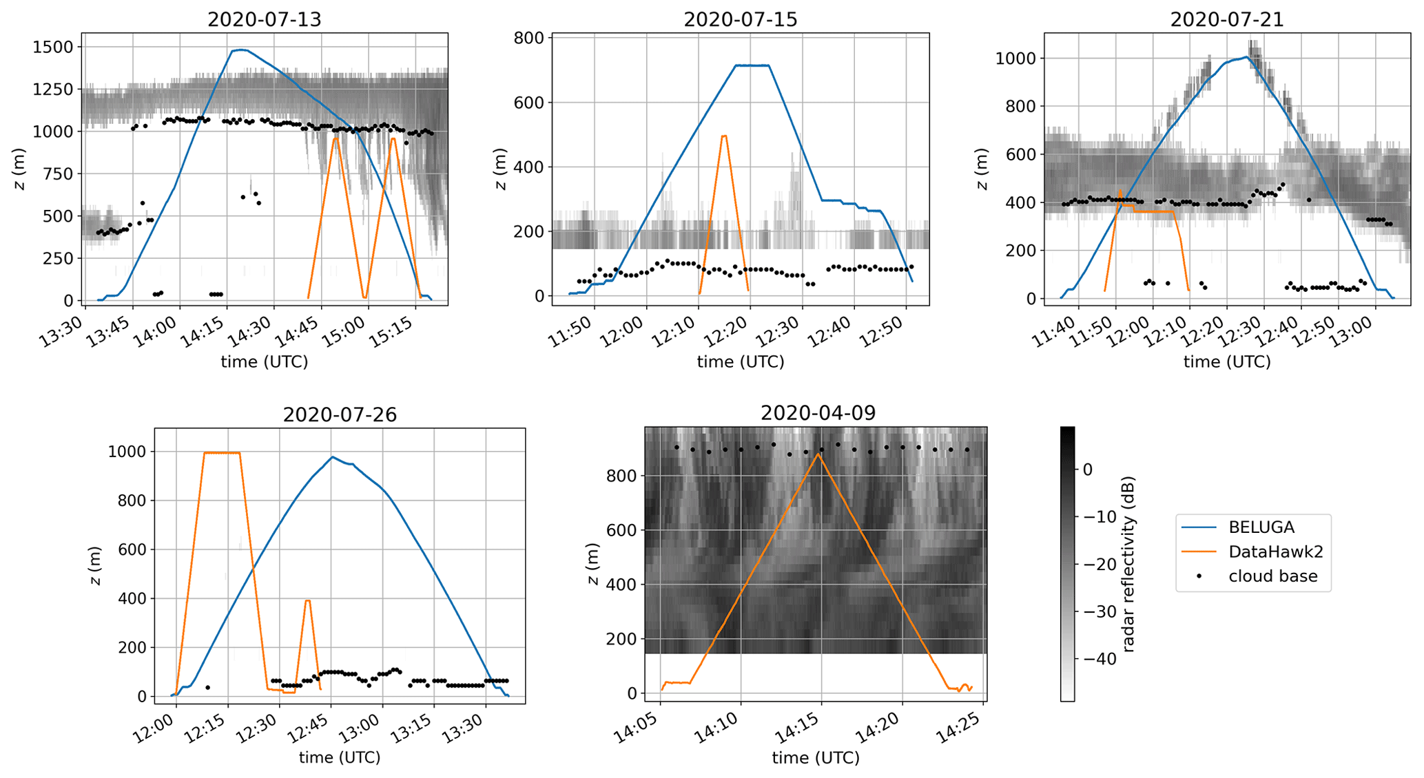
Figure 1Time–height profiles of DH2 and BELUGA flights for days presented in this paper. Days in July 2020 include the cases in which both platforms were operated simultaneously. Cloud base is from the RV Polarstern ceilometer (Schmithüsen, 2021). The gray shading shows radar reflectivity (Johnson et al., 2021). Note that the BELUGA balloon was observed by the radar during the case on 21 July 2020.
2.1.2 DH2 small uncrewed aircraft system
sUASs fill a niche in atmospheric observation, offering perspectives that are challenging to obtain with other in situ sensing methods. This includes an ability to fly in a variety of atmospheric conditions, some of which (e.g., fog, low aerosol concentrations, and no clouds/precipitation) can challenge traditional remote sensing techniques. sUASs can provide observations at altitudes from meters above the surface all the way up through the upper troposphere. Additionally, such platforms can provide high temporal and spatial resolutions and are able to resample a given layer of interest repeatedly. Their ability to sample horizontally also offers unique perspectives on spatial heterogeneity. While these platforms offer numerous advantages and can capture unique information, there are also constraints to their operation related to weather (e.g., winds, visibility, and icing conditions) and site-specific operational regulations.
The DH2 is instrumented to collect detailed information on the thermodynamic structure of the atmosphere while also simultaneously collecting data on winds and atmospheric turbulence. To observe the thermodynamic state, the system was equipped with a Vaisala RSS-421 pressure, temperature, and humidity sensor suite, with sensors extending into the streamflow passing over the aircraft. The platinum resistive temperature sensor on the RSS-421 offers 0.01 ∘C resolution and a repeatability of 0.1 ∘C with a 0.5 s response time at typical airspeeds. This sensor also includes a capacitive silicon pressure sensor offering 0.01 hPa resolution and a 0.4 hPa repeatability as well as a thin-film capacitive relative humidity (RH) sensor that offers a resolution of 0.1 % RH and a repeatability of 2 % RH. The response rate of the RH sensor is temperature dependent and ranges from approximately 0.3 s (at 20 ∘C) to 10 s (at −40 ∘C). In addition to the Vaisala sensor, the DH2 is equipped with a custom fine-wire array. This consists of 5 µm diameter platinum sensor wires, with one operated as a cold-wire thermometer and the other heated to serve as a hot-wire anemometer. The fine-wire array also includes a Sensirion SHT85 temperature and humidity sensor. A pitot-static probe serves as a reference for the hot-wire anemometer. Finally, the DH2 is equipped with (1) upward- and downward-looking IR thermometers that offer qualitative information on the surface state under the aircraft and the presence of clouds above the aircraft and (2) a custom-designed autopilot and associated sensor suite to measure aircraft attitude, position, and velocity. More details on the DH2 platform can be found in Hamilton et al. (2022).
During MOSAiC, this platform was operated semi-routinely from the expedition’s central observatory, near the frozen-in icebreaker RV Polarstern. The aircraft conducted frequent profiles to 1 km above the ice surface, operating in a spiral ascent–descent pattern while approximately maintaining a single geodetic location above the slowly drifting ice pack. Diameters of the spiral ascents and descents were 150 to 200 m, with a typical vertical rate of 2 m s−1. For this project, operations were limited to time periods when average winds were below 10 m s−1 and visibility was sufficient to maintain a visual line of sight to the aircraft in flight. This prevented the aircraft from flying in significant precipitation and/or through clouds. The DH2 was operated in very cold temperatures (down to −37 ∘C) and launched/landed on broken sea ice and melt-pond-covered surfaces. Despite weather challenges, the DH2 conducted a total of 82 flights during MOSAiC, compiling 42.9 flight hours of data over the central Arctic Ocean. Additional details on the MOSAiC DH2 deployment, including photographs of the aircraft, can be found in de Boer et al. (2022), and the data from these deployments are publicly available from the National Science Foundation (NSF) Arctic Data Center (Jozef et al., 2022b, 2021).
DH2 measurements of temperature, wind, and humidity were compared to those from the radiosondes as an established platform by Jozef et al. (2022a), who found that DH2 and radiosonde profiles of the aforementioned variables were similar to each other: features including ABL height, low-level jets, and inversions were in agreement between DH2 and radiosonde measurements taken at approximately the same time. Additionally, Hamilton et al. (2022) provide detailed statistics on the performance of the DH2 when compared to radiosonde observations within 1 h of the DH2 launch during MOSAiC, showing reasonable agreement of temperature and wind.
The pitot-static probe and the fine-wire sensors have been used in previous studies (e.g., Kantha et al., 2017; Balsley et al., 2018; Luce et al., 2019) to derive turbulent parameters such as the temperature structure parameter, eddy dissipation rate, and Ozmidov scale. Similarly, in the present study, we use the pitot-static probe and the hot-wire probe to derive the turbulent kinetic energy dissipation rate ε. The pitot-static probe, connected to a differential pressure sensor, is calibrated postflight as described by Doddi et al. (2022). The procedure for calculating horizontal winds from the pitot airspeed is also described in that study. The hot-wire airspeed cannot be calibrated directly to the pitot airspeed because the zero-voltage of the measurement circuit is adjusted in-flight to accommodate the measurement range. Therefore, hot-wire airspeed fluctuations are calibrated to pitot airspeed fluctuations in the spectral space for defined time intervals of 5 s. Figure 2 gives an example of a 5 s spectrum for pitot and hot-wire fluctuations. The pitot spectrum typically shows artifacts at frequencies above around 100 Hz due to motor vibrations and the electronics' noise floor, which have also been observed in previous studies (e.g., Luce et al., 2018). The spectral peaks from motor vibration are more pronounced on ascents. The DH2 uses a custom pitot tube with very short tubing to the pressure sensor so that no filtering of the airspeed signal is apparent up to the 400 Hz Nyquist frequency, beyond the anti-alias filtering roll-off seen at 300 Hz. As described in Doddi et al. (2022), estimates of ε only utilize the portion of the inertial subrange up to the vibration/noise floor artifacts in these spectra (indicated by the spectral average “Calibration points” in Fig. 2). The hot-wire spectra are much less distorted by motor vibrations than pitot spectra, but the hot-wire spectrum must be calibrated to the pitot spectrum with a calibration constant for each individual spectrum. This additional complexity was not warranted in the present study; therefore, turbulence parameters in this paper will be derived from the pitot airspeed, as discussed in Sect. 2.3.
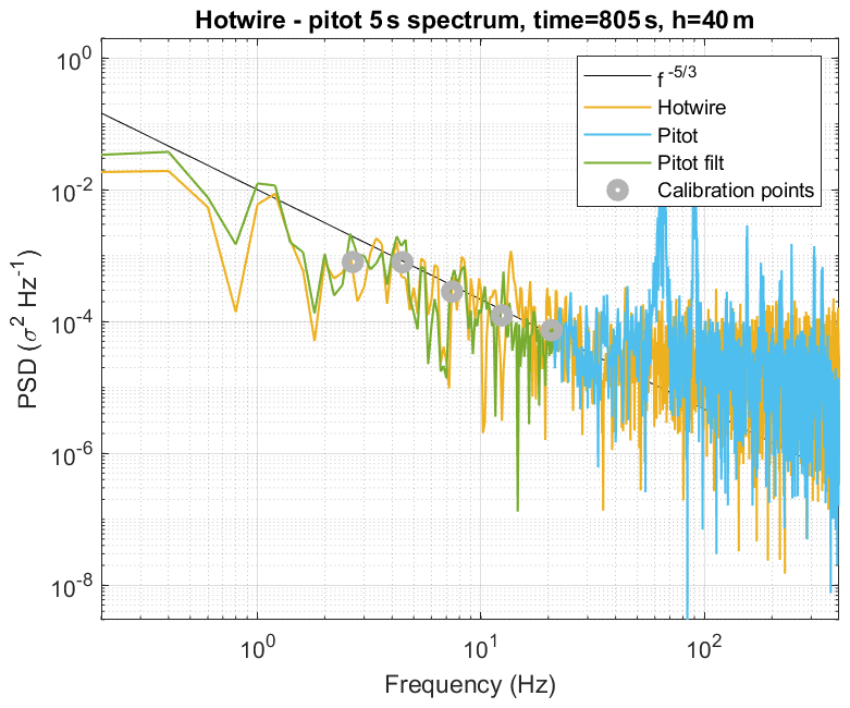
Figure 2Comparison of hot-wire and pitot spectra for one 5 s segment on 13 July 2020. The hot-wire fluctuations are calibrated to the pitot fluctuations in the frequency range marked by the gray dots (“pitot filt”).
2.1.3 Tethered balloon system
The BELUGA system operated during MOSAiC consisted of a 90 m3 helium-filled balloon attached to a winch via a 2 km tether. Multiple instrument packages were operated with BELUGA for vertical profile observations typically up to an altitude of 1 km. One profile lasted about 30 min at ascent and descent rates of 0.3–1 m s−1. BELUGA was operated below, inside, and above clouds at surface wind speeds below 7.5 m s−1 (Lonardi et al., 2022).
The main instrument used for this data analysis is an ultrasonic anemometer package including an attitude reference system. Using attitude angles and inertial velocities, the observed three-dimensional wind vector is transferred to an Earth-fixed reference system. The temporal resolution of the three-dimensional wind vector measurement is 50 Hz, which corresponds to a typical spatial resolution of 10 cm at a 5 m s−1 mean wind speed. An advantage of the ultrasonic system is the additional measurement of virtual temperature, which allows direct measurement of turbulent heat and momentum fluxes. The application and the limitations for turbulent flux estimates with BELUGA are discussed in Egerer et al. (2019a, 2021a).
2.1.4 Additional measurements
Vertical profile measurements at lower altitudes can be compared to near-surface meteorology and flux measurements from towers. The towers with nominal measurement heights of 2, 6, 10, and (temporarily) 23 m were mounted on the sea ice within 300–400 m distance of RV Polarstern (Shupe et al., 2022). These surface-based measurements provide a reference for flux magnitudes using a well-accepted ground-based eddy-correlation approach. Measurements of interest for this study were made by temperature and relative humidity probes and sonic anemometers mounted at several heights. The sonic anemometers operated at 20 Hz and were resampled to 10 Hz for analysis. Additionally, surface pressure was measured at a 2 m height, and 10 Hz measurements of water vapor concentration were made at 2 m (May 2020 and earlier) or 6 m heights (June 2020 and thereafter). Collectively, these measurements were used to derive surface sensible, latent, and momentum fluxes via the eddy-correlation technique at nominal 10 min intervals using 13.6 min segments of data (Cox et al., 2021). Measurements at 23 m height were only available during the period up until May. For the period starting in June, the meteorological tower was installed approximately 100 m from the BELUGA launch site during June–July.
Additionally, the Ka-band ARM Zenith Radar (KAZR) was operated by the US Department of Energy (DOE) Atmospheric Radiation Measurement (ARM) program onboard RV Polarstern (Johnson et al., 2021). It provided continuous vertical measurements of the radar reflectivity, mean Doppler velocity, and spectral width, which collectively provide information on the vertical distribution of clouds, the type of clouds, and the presence of turbulent mixing in the atmosphere. The radar and mast measurements serve as a reference and for putting the DH2 measurements into context.
2.2 Flux gradient method and turbulent exchange coefficient
The flux gradient method (Stull, 1988), as a first-order local turbulence closure scheme, relates local gradients to respective turbulent fluxes. Using this method, turbulent fluxes (e.g., the turbulent sensible heat flux ) can be approximated from vertical profiles of mean parameters (marked with an overline) using the mean vertical potential temperature gradient :
The turbulence exchange coefficient for heat KH must be parameterized as a function of the flow. Commonly, the parameterizations are formulated for the turbulent exchange coefficient of momentum Km (Holt and Raman, 1988), which is related to KH via the turbulent Prandtl number Prt:
Similarly, the turbulent latent heat flux is related to the mean profile of specific humidity q with KQ≈KH (Dyer, 1967) and the mean humidity gradient :
The flux gradient method is one of the simplest turbulence parameterizations and is particularly suited for small eddies (Stull, 1988). The presence of larger-sized eddies and counter-gradient fluxes might cause the method to fail. However, a local closure scheme (where K is a local estimate) might be best suited to describe a nonclassical, complex ABL with, for example, multiple inversions.
A large number of parameterizations for Km have been developed (e.g., Bhumralkar, 1976; Mahrt and Vickers, 2003; Cuxart et al., 2006) and are widely used for sub-grid turbulence in numerical models. Some of the parameterizations are derived from or validated against airborne measurements (e.g., Bélair et al., 1999; Aliabadi et al., 2016). The main method for the K parameterization used in the present work is based on the work of Hanna (1968), who suggested parameterizing K based on local turbulence parameters of the vertical velocity spectrum. The study, based on dimensional reasoning, hypothesizes that K can be parameterized by the quantities determining the turbulent energy spectrum of vertical wind velocity: standard deviation of vertical wind velocity σw, eddy dissipation rate ε, and the wavelength of the peak in the wind velocity energy spectrum. As these parameters interdepend on one another (Hinze, 1975), two out of the three are sufficient to determine K. Applying this parameterization allows one to deduce turbulent fluxes from vertical profiles of the measured turbulence parameters σw (or variance ) and ε. Km is related to σw and ε by
leading to
The turbulent Prandtl number Prt can be approximated (Sect. 2.3.4); C is a constant with C=0.35 for nearly neutral conditions. In the original paper, the parameterization is validated by different observational data over land and sea from towers and aircraft under various stability regimes in the ABL up to 320 m height.
With the parameterized turbulent exchange coefficient, the turbulent fluxes of heat and moisture are as follows:
Here, ρ is the air density, cp is the specific heat capacity of air, Lv is the latent heat of vaporization, and KQ≈KH is assumed. The method by Hanna (1968) has been used for a wide range of applications. It is often adopted for air pollution modeling (Tomasi et al., 2019; McNider and Pour-Biazar, 2020) and has also served to calculate particle fluxes based on sUAS data (Platis et al., 2016). The method has even been extended to ABL conditions in a tropical cyclone (He et al., 2021) using tower observations and to hurricane conditions in the low-level troposphere (Zhang et al., 2010) using aircraft observations.
To apply the Hanna (1968) parameterization, some assumptions have to be made. First, Prt is a function of stability (Li, 2019): heat transport is suppressed under stable conditions through buoyancy effects. Different formulations exist for how Prt varies depending on different stability parameters, and a relationship has to be selected based on available data and conditions (see discussion in Sect. 2.3.4). Second, the constant C has to be determined from observations and also depends on stability. The original value C=0.35 is based on a variety of stability conditions (Hanna, 1968; Busch and Panofsky, 1968). Subsequent studies have shown that C is closer to 0.41 for stable conditions (Nieuwstadt, 1984; Lee, 1996). Here, we use C=0.41, as we analyze mostly stable conditions. Last, it matters if the turbulence parameters in Eq. (4) are estimated from velocity fluctuation measurements transverse to (e.g., w components) or along (u component) the mean flow. In isotropic turbulence, the statistical properties of the flow are independent of the direction in which they are measured. Because atmospheric turbulence is predominantly anisotropic, especially at larger scales (e.g., Lovejoy et al., 2007; Biltoft, 2001), this has to be considered when measuring turbulence. The next section introduces the DH2 measurements and how they can be applied with the flux gradient method, and it also discusses the assumptions mentioned above.
2.3 Application of the flux gradient method to DH2 measurements
The DH2 provides measurements of the one-dimensional horizontal airspeed with a pitot-static probe and a hot-wire anemometer at a sampling frequency of f=800 Hz. These measurements provide the foundation to apply the flux gradient method with the K parameterization by Hanna (1968) based on the turbulence parameters dissipation rate (ε) and wind velocity variance (σ2). Fluctuations in the measured airspeed of the pitot and hot-wire probe correspond to longitudinal measurements of the three-dimensional wind velocity field. Due to the small slant-path angle of the helical flight resulting from the ∼2 m s−1 ascent–descent rate and ∼15 m s−1 airspeed, we consider these to be approximate horizontal measurements.
2.3.1 Dissipation rate
The turbulent energy dissipation rate ε is of central importance in describing turbulent flows. Muschinski et al. (2004) and Siebert et al. (2006) discuss different methods for estimating local dissipation rates from airborne in situ measurements. Most commonly, ε is derived either from the energy spectrum or from structure functions. Both techniques estimate dissipation rates from measurements at inertial subrange scales.
The spectral method is based on the turbulent energy spectrum of lateral or longitudinal wind velocity fluctuations in a defined time period. In the inertial subrange, the longitudinal energy spectrum has the following universal form:
(Kolmogorov, 1941) with the energy dissipation rate ε, wave number , mean horizontal airspeed , and the universal Kolmogorov constant α≈0.5 for the longitudinal wind velocity spectrum (Högström et al., 2002; Yeung and Zhou, 1997). A fit to the energy spectrum of a measured time series segment provides a local ε.
Structure functions are based on the velocity increment between two measurement points at times and t. By evaluating the structure function for a discrete time series of a flow velocity component, the dissipation rate can be retrieved. Siebert et al. (2006) concluded that the second-order structure function provides the most robust results for estimating local dissipation rates from observational data. We estimate local dissipation rates ε from the second-order structure function for the longitudinal wind component u
in a defined time period with C2≈2 for the longitudinal flow component. Averaged parameters in Eq. (9) are indicated by an overline, u(t) is the horizontal wind velocity at the time t, and t* is a time lag. The structure function can also be applied to the vertical wind component w with C2≈2.6 for lateral velocity components (Pope, 2000).
The DH2 turbulence dissipation rates are derived from high-resolution pitot airspeed fluctuations following the turbulence spectral analysis presented in previous publications (Frehlich et al., 2003; Luce et al., 2018, 2019; Doddi et al., 2022). The dissipation rates are computed by fitting the measured one-dimensional airspeed frequency power spectra to the model universal turbulence energy spectrum E(k) (Eq. 8) in the inertial subrange characterized by a slope (Kolmogorov, 1941). Taylor's frozen flow hypothesis (Pope, 2000) is invoked to approximate the temporally measured DH2 one-dimensional airspeed power spectra as wave number spectra, thereby enabling model spectral fitting. First, the pitot-measured airspeed data are segmented into 5 s interval time records. The time records are detrended and subsequently windowed by a variance-preserving Hanning window. A fast Fourier transform algorithm is implemented to compute energy spectra of the windowed time records and normalized to obtain the one-dimensional airspeed power spectral density (PSD). The pitot-measured airspeed is contaminated by aircraft-motor-vibration-induced periodic artifacts that appear as sharp peaks in spectra at high frequencies (see Sect. 2.1.2 and Fig. 2). The average PSD in equally spaced logarithmic frequency bins is computed to reduce the spectral variance and aid in identifying the motor-induced periodic artifacts. The mean and standard deviation of the -weighted spectra are calculated in a frequency range that avoids the prominent periodic artifacts. The turbulence dissipation rates including error bars are estimated from the spectral fit mean and standard deviation using Eq. (5) in Luce et al. (2019) and Eq. (30) in Frehlich et al. (2003). Doddi (2021) presents the details of the DH2 pitot spectral analysis procedures outlined above and careful consideration of the assumptions involved in turbulence spectral analysis. Here, the results of the spectral method are dissipation rates derived from pitot airspeed fluctuations. The hot-wire provides comparable dissipation rates to the pitot because the hot-wire spectrum for each segment is fitted to the pitot spectrum; however, the varying hot-wire calibration coefficient influences the results. Figure 3 shows a vertical profile of ε for a day where the hot-wire calibration was reliable. The spectral methods for pitot and hot-wire (black and red crosses, respectively) show a very similar vertical structure and magnitude.
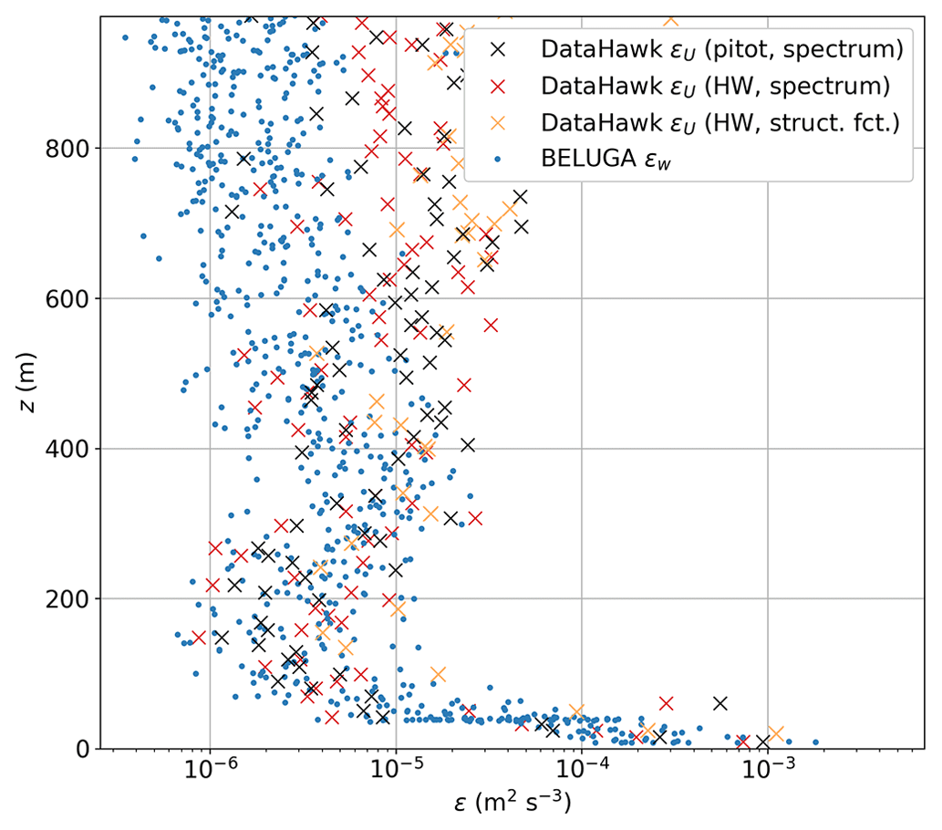
Figure 3Comparison of different methods for calculating ε (subscripts indicate the wind component that ε was derived from): vertical profile (ascent) for 26 July 2020. For DH2, ε is derived using the spectral method from pitot and hot-wire measurements and applying the second-order structure function method to hot-wire measurements for comparison with BELUGA. ε for BELUGA is derived using the second-order structure function for the vertical wind velocity component w.
For BELUGA, the dissipation rates are derived from the second-order structure function (Egerer et al., 2019a, 2021a; Lonardi et al., 2022). For defined time segments, the structure function on the left side of Eq. (9) is evaluated for time lags t* in an empirical time range of . Fitting this curve to the right side of the equation yields ε for each time period. Exponents (that should theoretically equal ) are accepted in a range of 0.3 to 0.9, otherwise no dissipation rate can be estimated. Values of ε can be estimated from any spectral range in the inertial subrange in Eq. (9); hence, time periods for applying this equation can be short, and periods of 2 s length are selected to be consistent with previous studies (Egerer et al., 2019a, 2021a). As the sonic anemometer provides the three-dimensional wind vector, dissipation rates can be estimated from both the horizontal and vertical wind components. For BELUGA, the vertical wind component is used because of the higher measurement resolution. However, Hanna (1967) found it easier to determine ε from the horizontal component rather than from the vertical and found the relation (indices of ε indicate the wind vector component it was derived from) near the ground with similar values higher up. Anisotropy might be responsible for a difference in εu and εw and will be further discussed in Sect. 2.3.5.
For BELUGA and DH2, different established methods are used because they are suited to the individual characteristics of the respective measurements in terms of distinctive features in the spectra, measurement resolution, etc. To exclude errors resulting from the two different methods, they are compared by also applying the structure-function approach to the DH2 data. Because of the artifacts in the pitot fluctuation time series, hot-wire fluctuations restored from the fitted spectra are used. This is possible for the 26 July flight, which had few variations in the hot-wire calibration constant. The results in Fig. 3 suggest that both the structure function and spectral method provide similar ε results for the DH2. The spectral method for pitot will be used as the default method for the DH2. The results for BELUGA are added for comparison, showing a comparable vertical structure with a similar magnitude of ε. BELUGA dissipation rates agree very well with DH2 values below 600 m altitude. Above, the results from the two platforms deviate from each other, which might be caused by the spatial distance between them. However, BELUGA cannot resolve values below around m2 s−3, because the sonic anemometer on BELUGA has a lower measurement resolution limit (influenced by the sampling frequency and noise floor).
Dissipation rates for BELUGA and DH2 are further compared for all flight times when both platforms operated simultaneously (flights on 12, 15, 21, and 26 July 2020; see Fig. 1), covering a large range of turbulence intensities. Figure 4 compares averaged dissipation rates in 10 m height bins (ascents and descents) for both platforms and ε for BELUGA derived from the vertical and horizontal wind component. All data points as a whole show a clear, near-linear relation between DH2 and BELUGA dissipation rates. εu from the DH2 seems to fit better with εw from BELUGA. This might be due to the fact that BELUGA has a lower resolution for the horizontal component and does not resolve smaller ε for this component. However, when comparing different measurement platforms, one should consider the spatial distance and time difference between the observations in potentially fast-changing ABL conditions.

Figure 4Comparison of dissipation rates ε for BELUGA and DH2 for all concurrent fight times. Each data point represents a 10 m height interval with averaged ε for the daily data shown in Fig. 1. For BELUGA, dissipation rates are calculated for the horizontal wind component u and the vertical component w. The black line represents the 1:1 relation.
2.3.2 Wind speed variance
The variance of a wind velocity component is needed, along with the turbulent dissipation rate, to apply Eq. (4). For the DH2, the hot-wire wind velocity fluctuations would be most suitable to calculate variances in discrete time segments, as the hot-wire is less disturbed by motor vibrations than the pitot. However, the highly variable hot-wire calibration can cause artificial variance. On the other hand, the distortions in the pitot airspeed data do not allow a simple variance estimation from time series segments, as the high-frequency spectral peaks create artificial variance as well.
Therefore, variances are calculated by integrating the pitot airspeed power spectra over frequencies that exclude the spectral artifacts. The power spectra are calculated for 5 s intervals (an example is given in Fig. 2). A low-pass spectral filter is applied to exclude the high-frequency peaks due to motor vibrations. The cutoff frequency for the low-pass filter varies for each individual spectrum depending on the frequency range of the spectral peaks and is determined as outlined in the following. After detecting the noise floor in the spectrum, an slope is fitted to frequency-binned data points above the noise floor. The standard deviation from this curve is then calculated, starting with the lowest-frequency points. If subsequent points deviate more than 10 % of the standard deviation, these points are excluded. The highest frequency of the “valid” data points is the cutoff frequency up to which the spectral variance is calculated. The cutoff frequency is commonly above 10 Hz (in the example spectrum in Fig. 2, the cutoff frequency is 35 Hz). Each 5 s spectrum provides one value for its variance. The consistent 5 s interval for calculating both dissipation rates and variances was chosen as a compromise between resolving the vertical profile and including as many scales of the energy spectrum as possible for calculating variances. With the relatively short averaging time for variances, we exclude lower frequencies in the spectrum; however, we aim to resolve a vertical profile and the turbulent exchange between shallow layers in the ABL. A comparison of different DH2 averaging intervals shows an expected decrease in resolution with increasing averaging time, yet the magnitude of the variance increases only slightly relative to the range in variance across a vertical profile. Therefore, we assume the 5 s interval to be sufficient for the purpose of this study.
For BELUGA, variances are derived directly from time series segments for one wind velocity component as outlined in Egerer et al. (2019a). Turbulent fluctuations are separated from the larger-scale ABL structure by applying a high-pass 20th-order Bessel filter with a filter window of typically 10–50 s length. Variances are calculated in a rolling window on the vertical profile. The selected filter window determines the included scales and, therefore, the magnitude of resulting variances. In Fig. 5, filter windows of 5, 15, and 30 s are tested for BELUGA variances on a vertical profile for the vertical wind component w. Although the variance estimate grows with time window length, the increase (e.g., between 5 and 15 s windows, about a factor of 2) is small relative to the range in variances typically seen over altitude (nearly 2 orders of magnitude in this case). Instead, the window mainly determines the vertical resolution of the variance. To compare the BELUGA method to DH2 variances, Fig. 5 adds BELUGA variances calculated from 5 s detrended time series segments (as used for DH2 spectrally derived variances). This is equivalent to spectral variances without applying any filter. The observed structure in the vertical profile agrees well for rolling variances in different window sizes and the 5 s detrended segments, although the detrended segments show slightly higher variances. The magnitude seems to agree well with a 15 s rolling filter window. As a result, variances for BELUGA are calculated with a 15 s window high-pass filtered time series. Note that because the airspeed of the DH2 is about 15 m s−1 and the typical wind speed measured by BELUGA is about 5 m s−1, using a 5 s analysis window for DH2 measurements would be equivalent to a 15 s analysis window for BELUGA measurements in terms of the wind field scales included in the variance estimates. The variance derived from DH2 measurements, as described above, are added in Fig. 5. The general magnitude and vertical structure compare well to BELUGA measurements, but the DH2 variances fluctuate more. The differences in Fig. 5 might be due to the varying cutoff frequency or undetected spectral peaks in the DH2 estimates or to the fact that the DH2 samples over a larger spatial domain transverse to the mean wind compared with BELUGA.
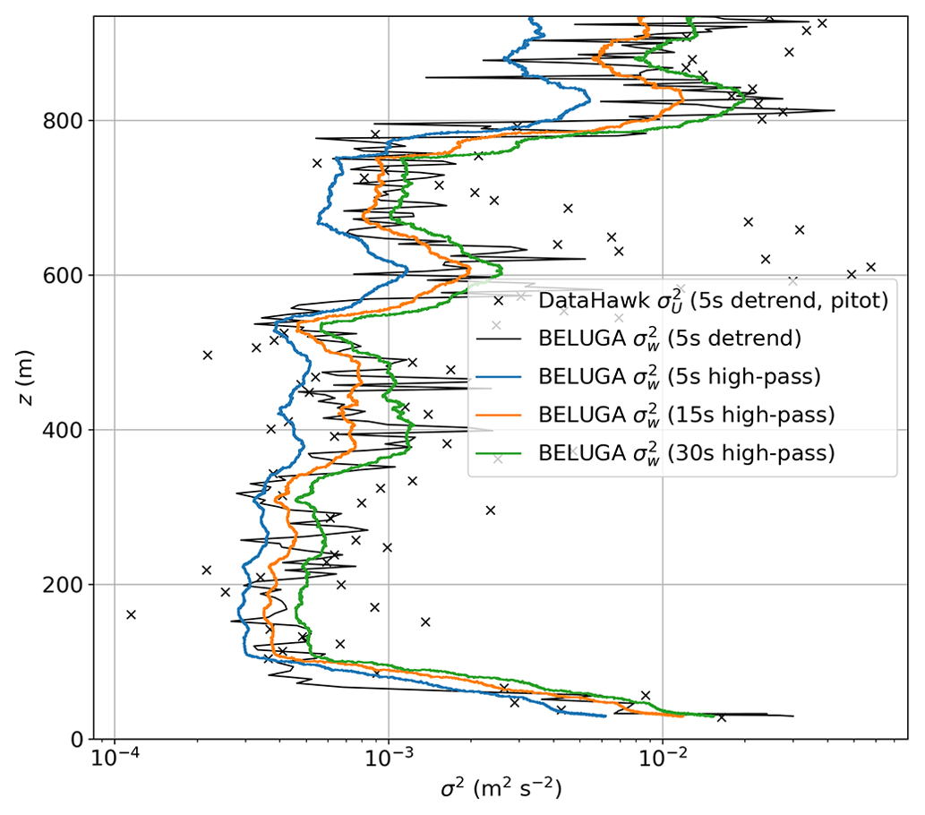
Figure 5Comparison of different methods for calculating wind velocity variances σ2: vertical profile (first descent) for 13 July 2020. The black line represents BELUGA variances calculated from nonoverlapping, detrended 5 s segments. The orange, blue, and green lines show BELUGA variances calculated in rolling windows after applying different high-pass filters to the time series. The black crosses result from DH2 5 s pitot, filtered spectra, as described in the text.
Figure 6 compares DH2 and BELUGA variances for all concurrent flights, similar to Fig. 4 for dissipation rates. For BELUGA, variances are calculated for the horizontal and vertical wind components. The resolution limit (noise floor) for the horizontal component is higher; therefore, values for m2 s−2 are locked to a value near the noise floor level of around m2 s−2. The influence of the measurement resolution limit is more obvious for variances than for dissipation rates. Above the BELUGA resolution limit, there is a correlation between DH2 and BELUGA variances across all variance levels, despite the inevitable spatial and temporal differences in the measured parameters.

2.3.3 Richardson number
Stability is of central importance to describe the vertical structure of the ABL and is used in this study for parameterizations of the turbulent Prandtl number and anisotropy. Different parameters exist to describe the stability of a flow, such as the bulk, gradient, and flux Richardson numbers or the Monin–Obukhov length. In this study, we use the gradient Richardson number as a stability parameter. This number can describe the ABL structure locally (e.g., in the case of multiple inversions) because it does not depend on surface conditions. Further, it can be derived from vertical profile measurements of mean parameters. The gradient Richardson number represents the ratio of buoyancy (with the Brunt–Väisälä frequency N) to wind shear S:
When calculating local wind and temperature gradients for Rig on the vertical profile, the measured temperature and wind profiles must be averaged in a defined time window. For BELUGA, a 20 s window is selected to provide a 10 m vertical resolution at climb speeds of around 0.5 m s−1. DH2 ascends and descends at around 2 m s−1. Although the corresponding time interval for the equivalent vertical resolution would be 5 s, a 10 s averaging window for temperature is selected as a compromise between vertical resolution and horizontal averaging on the flight pattern circles. Different from temperature, the DH2 wind profile is averaged over 20 s to exclude artifacts from wind changes on the helix flight pattern and from extreme bank angle changes for both platforms, outliers are excluded on the resulting Rig profile, and the profile is again smoothed to reduce artifacts. Figure 7a shows a distribution of derived Rig for DH2 and BELUGA for 1 d during MOSAiC. For both platforms, the distribution of Rig peaks at values just above zero and shows a comparable density distribution. The DH2 distribution is slightly flatter than the one for BELUGA. However, the Ri-outlier problem (Sorbjan and Grachev, 2010) – the ratio of very small gradients is ambiguous and it becomes hard to differentiate stable and low-wind conditions – is especially present under the conditions encountered in the Arctic. Therefore, large Rig values have to be treated with caution. A critical Richardson number value Ric between 0.25 and 1 (Miles, 1961; Abarbanel et al., 1984) is assumed to differentiate conditions with weak stability (Ri<Ric) and strongly stable conditions (Ri>Ric). Values for Rig in Fig. 7a cover both stable and unstable conditions. However, turbulence can still be present beyond Ric (Sukoriansky et al., 2006), as has been shown by a large number of meteorological and oceanographic observations (e.g., Kondo et al., 1978; Yagüe et al., 2001; Mack and Schoeberlein, 2004). Further, Jozef et al. (2022a) found that a value of Rig=0.5 to 0.75 on the vertical profile can be used to determine the ABL height based on DH2 MOSAiC data.
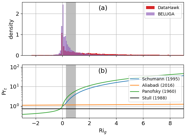
Figure 7Histograms of (a) all measured gradient Richardson numbers Rig for BELUGA and DH2 for flights on 13 July and (b) different parameterizations for Prt=f(Rig). The range of critical Richardson numbers is shown using gray shading.
2.3.4 Turbulent Prandtl number
The turbulent Prandtl number Prt describes the ratio of momentum transfer to heat transfer and is used in this work to apply the parameterization in Eq. (4) to turbulent heat transport. Prt is a function of the flow itself and, more precisely, of the stability of the flow. The controversy about a quantitative description of Prt in relation to a stability parameter is still ongoing (Li, 2019; Grachev et al., 2007). Most studies agree that Prt≈1 is close to unity for turbulent flows that are often associated with Ri<Ric. The behavior of Prt for stable flows is less clear, which is obvious given that the definition of Prt (Eq. 2) presumes the existence of turbulence implicitly. For stable flows, the behavior of Prt also depends on the selected stability parameter. Many studies agree that Prt increases with increasing stability when plotting Prt versus the gradient Richardson number Rig (Kondo et al., 1978; Kim and Mahrt, 1992; Yagüe et al., 2001; Monti et al., 2002; Galperin et al., 2007). Grachev et al. (2007) found that Prt increases with increasing Rig but decreases with increasing flux Richardson number Rf, surface-based bulk Richardson number, and the Monin–Obukhov stability parameter (all measures for increasing stability), although using the same data. Yagüe et al. (2001) found no clear stability dependence when using as a stability parameter. Opposed to other studies, Sorbjan and Grachev (2010) found that Prt decreases with Rig. According to Howell and Sun (1999) and Grachev et al. (2007), Prt is even less than one when plotted against the Monin–Obukhov stability parameter.
In this study, we rely on Rig as a stability parameter, even though it is prone to self-correlation and the Ri-outlier problem (Grachev et al., 2007). Other parameters such as and the surface-based Rib assume a classical ABL and do not cover more complicated structures such as multiple inversions. Li (2019) compare different relations of Prt to Rig and conclude that a number of field and laboratory experiments and numerical simulations show an increasing, asymptotic behavior of Prt with Rig under stable conditions in the form of (Bange and Roth, 1999; Vasil'ev et al., 2011; Aliabadi et al., 2016). The study also compares two analytical functions for the relationship based on direct numerical simulations (Venayagamoorthy and Stretch, 2010) and large-eddy simulations (LESs) for laboratory experiments (Schumann and Gerz, 1995), which agree well with experimental data from other studies. These functions are close to an earlier formulation of Panofsky et al. (1960), which is used in Hanna (1968). Figure 7b compares the different formulations to the simplified constant value of Prt=0.7 (Stull, 1988).
Because most of these studies are tied to very specific conditions often confined to the surface layer, we use the Prt–Rig relation of Aliabadi et al. (2016). This relation was derived in clear-air turbulence in the Arctic lower troposphere using aircraft measurements up to a 3 km altitude. Different stability regimes including counter-gradient fluxes were covered, yielding the following formulation:
where a=0.89 and b=0.01 (Fig. 7b). We use this parameterization because it is based on the suitable parameter Rig and on airborne measurements in the Arctic exceeding the surface layer; moreover, it is a conservative estimate between other parameterizations and the simplified assumption Prt≈0.7.
Hence, the DH2 provides the necessary measurements of T, , and ε to estimate the turbulent heat flux. It remains open that the DH2 airspeed measurements represent the near-horizontal vector component of velocity fluctuations (due to the small slant-path angle), whereas the vertical component is needed for the method discussed above. Therefore, the next section examines anisotropy of these fluctuations.
2.3.5 Anisotropy
Turbulence properties in the ABL behave differently depending on their orientation in the flow field. Isotropy is more likely to be found at smaller scales, and the scales at which a flow becomes anisotropic is influenced by stability and other factors. Generally, anisotropy is favored by strong stability (with low turbulence), and horizontal modes dominate in anisotropic flows with high Richardson numbers (Mauritsen and Svensson, 2007). Galperin et al. (2007) showed that turbulence in an otherwise stable environment is influenced by anisotropy and internal waves. Anisotropy also depends on the height above the surface: close to the surface, horizontal mixing becomes dominant due to the spatial limitations of vertical eddies.
The K parameterization in Sect. 2.2 is based on the vertical velocity spectrum, but the DH2 turbulence estimates are based on the horizontal wind component u. The slant profiles are assumed to provide horizontal measurements because of the small effective angle to the horizontal plane of around 8∘. When using the DH2 measurements, isotropy cannot be assumed, as the stable ABL is predominantly anisotropic (particularly at larger scales), with the horizontal component dominating. Therefore, we aim to describe anisotropy depending on a stability parameter so that the vertical wind turbulence estimates in Eq. (5) can be replaced by the horizontal turbulence estimates measured by the DH2. While some studies describe a qualitative relation of anisotropy and stability (Mauritsen and Svensson, 2007; Nowak et al., 2021), no quantitative parameterization of these parameters exists (to the authors' knowledge). This is reasonable because anisotropy depends on many influence factors beyond stability, especially near the surface, and cannot be entirely parameterized. However, finding an empirical correlation between anisotropy and layer stability provides a useful way to predict when anisotropy could be expected. For this approximation, we use available MOSAiC data from BELUGA and examine anisotropy through ratios of directionally derived quantities, resulting in anisotropy coefficients A for variances and dissipation rates:
We use Rig as the stability parameter. While the coefficients and Aε are well suited to describe anisotropy in stronger turbulence, the quotient of small values for w and u becomes prone to errors for strong stability with weak turbulence. BELUGA measurements are consulted for the sought-after parameterization because they provide co-located estimates for variances and dissipation rates derived from both horizontal and vertical wind velocity components and data are collected on a vertical profile. While meteorological towers provide the same sort of measurements, these are obviously influenced by the surface, which complicates the comparison to the DH2 profile measurements. All BELUGA flights during MOSAiC are considered for the anisotropy description. To verify a more universal relation, further data from a previous BELUGA campaign on Arctic sea ice in 2017 are included (Physical feedbacks of Arctic planetary boundary level Sea ice, Cloud and AerosoL – PASCAL; Egerer et al., 2019a; Wendisch et al., 2019).
Figure 8 shows results for the relation of and Aε to Rig in the form of box plots for discrete Rig bins. In Fig. 8a, data from the two included campaigns agree well for variance anisotropy ratios and show more anisotropy (with dominant horizontal fluctuations, meaning ) for stronger stability (high Rig) and closer to isotropy () for weaker stability (Rig<0.25). Under very unstable conditions (Rig<0), decreases again. For Aε, the data are more scattered and agree less between the two campaigns (not shown), but they still show a similar shape of the distribution. If all campaign data are plotted together, a root function for both the –Rig and Aε–Rig relation can be fitted to the means of the box plots. These relations (shown in Fig. 8b) are used with the DH2 horizontal measurements to provide turbulence parameter estimates of the vertical spectrum based on the measured horizontal spectrum and Rig. Applying these anisotropy–stability relations from BELUGA measurements enables DH2 measurements in Eq. (4) to be used to calculate vertical flux profiles.
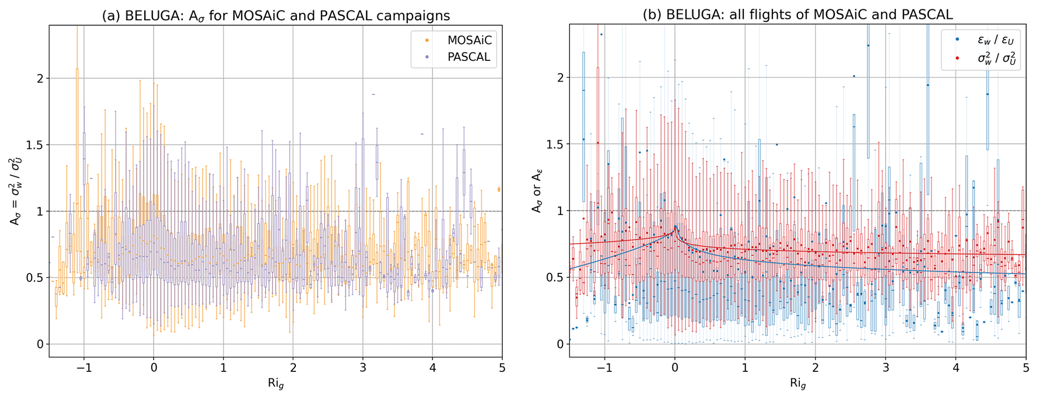
Figure 8Anisotropy in relation to stability (expressed by Rig) from BELUGA measurements for the MOSAiC and PASCAL campaigns: (a) comparison of anisotropy for variances segregated between MOSAiC and PASCAL data and (b) anisotropy for variances and dissipation rates from all MOSAiC and PASCAL data. The box plots for each Rig interval include the first quartile to the third quartile of the data, with a line at the medians and a dot at the means. The mean values are used to fit a function of the form (the function is fitted to a version of the plot with a more highly resolved Rig).
This section presents DH2 vertical profiles for three case studies with different ABL conditions. Two cases were obtained in July 2020, with concurrent measurements from DH2 and BELUGA. During the first case, clear-sky ABL conditions on 26 July were shaped by a strong persistent high-pressure system over the Barents Sea and a significant warm and moist air intrusion from the southeast (Lonardi et al., 2022). In contrast, on 13 July a high-pressure system over the North Pole caused colder and calm conditions with a liquid cloud layer (Lonardi et al., 2022). The third case on 9 April with a single-layer, mixed-phase cloud is associated with an anomalously cold period associated with air masses coming from the north (Rinke et al., 2021).
3.1 The 26 July 2020: stably stratified ABL with weak turbulence
Many of the DH2 measurement days during MOSAiC are characterized by stable stratification of the ABL. The 26 July case is one example of these conditions and is selected for analysis because of concurrent measurements of DH2 and BELUGA up to 1000 m. Generally, this day experienced clear-sky conditions with some intermittent low-level fog or haze near the surface evident in radar data. Lidar data occasionally show very thin high clouds formed in aerosol-rich layers probably without significant impact on the lower atmospheric structure. Both DH2 and BELUGA measurements up to 1000 m (Fig. 9) show a similar ABL structure with a surface-based temperature and humidity inversion between the surface and 200 m. Above the inversion, the ABL is slightly stable throughout the profile with nearly constant q. The air mass is warm and moist with potential temperatures up to 20 ∘C and q between 5 and 6 g kg−1. Wind speed is also fairly constant throughout the profile, not exceeding 5 m s−1 below 800 m. Meteorological measurements from both platforms agree well with the radiosonde and tower measurements.
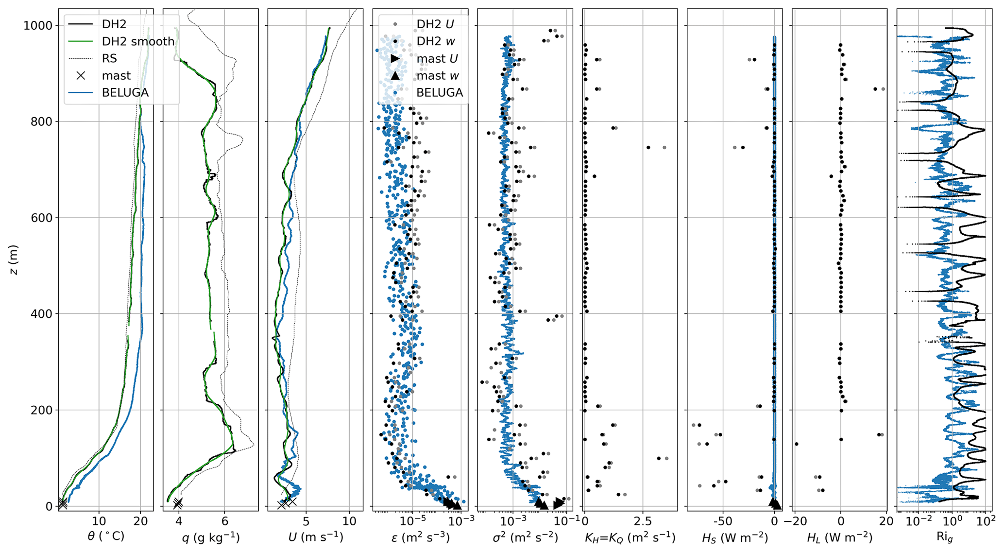
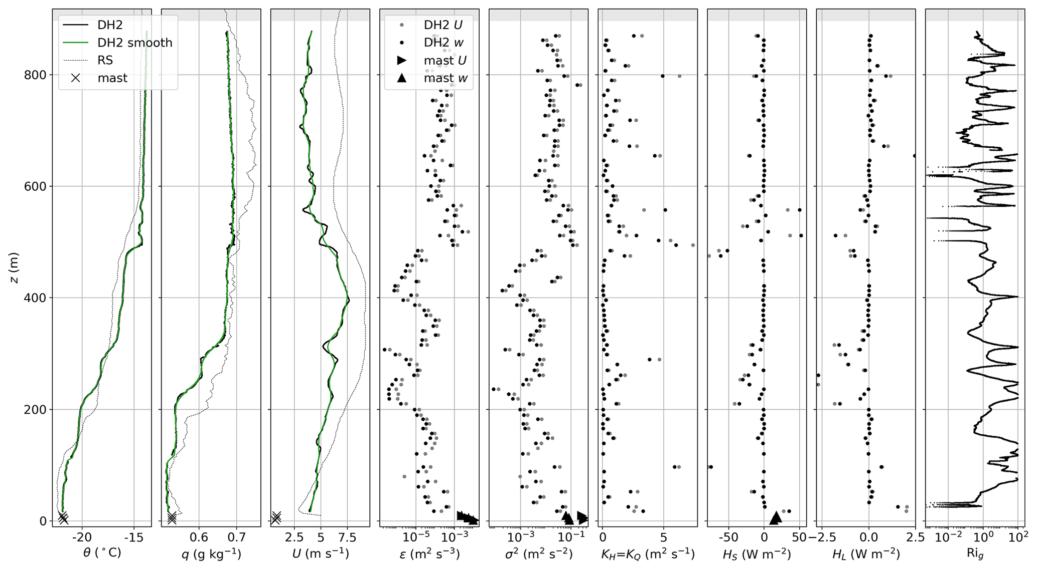
Figure 9Vertical profiles for 26 July (first ascent) for DH2 (black lines and dots) and BELUGA (blue lines and dots) with radiosonde (thin dotted lines) and tower (crosses and triangles near the surface) measurements as reference. The panels show potential temperature θ, specific humidity q, horizontal wind speed u, dissipation rate ε, wind speed variance σ2, turbulent exchange coefficients KH and KQ, turbulent heat fluxes of sensible heat HS and latent heat HL, and gradient Richardson number Rig. The green lines show the smoothed DH2 profiles for gradient calculations. The gray dots for ε, σ2, K, and flux values are derived from horizontal DH2 measurements without anisotropy correction.
Dissipation rates and wind speed variances indicate surface-induced turbulence within the inversion layer. Above the inversion, turbulence gets very weak with values of m2 s−3. At this point, the BELUGA measurements fall below the sonic instrument's noise level, which becomes evident from the barely varying values throughout the profile. DH2 shows more ε and σ2 variations within several layers of tens of meters thickness. The fourth and fifth panels in Fig. 9 for ε and σ2, respectively, also compare the DH2 “horizontal” direction (actual slant profile measurements) and “vertical” direction (measurements corrected with the anisotropy relation in Sect. 2.3.5). The difference between those directions (corresponding to the anisotropy factor in Fig. 8) is much less than the variation between the turbulent surface layer and the stable layer above (equal to 2 orders of magnitude); the general profile is not altered by using either of the directions. Anisotropy close to the surface is also reflected in the tower measurements: these show higher variances (by almost 1 order of magnitude) for the horizontal direction than for the vertical direction because of larger-scale fluctuations included in the 13 min averaging interval. DH2 and BELUGA do not cover these larger-scale fluctuations due to their measurement principle (the averaging interval is restricted on the vertical profile). For the mast dissipation rates, horizontally and vertically derived values are similar because ε is a measure of energy dissipation at small scales in the inertial subrange which are more isotropic. The turbulent exchange coefficient K is close to zero throughout the vertical profile (due to the low turbulent motions) but increases near the surface. This also applies to sensible and latent heat fluxes: these are close to zero throughout the profile and turn negative inside the inversion. Here, enhanced turbulent motions mix heat and moisture downward along the mean temperature and humidity gradients. The larger flux values are associated with more scatter. The BELUGA sensible heat flux profile looks similar, although with smaller flux values in the inversion. This is probably caused by the limited averaging time of 10 s for the covariances. However, the mast flux magnitudes with the 13 min averaging time indicate a negative flux with similar magnitude at 11 m height and slightly positive fluxes below. Gradient Richardson numbers are below Ric close to the surface, matching the turbulence profiles. In the stable region above, Rig indicates several thin layers of increased turbulence. These might be natural or a result of the quotients of shallow temperature and wind velocity gradients. To conclude, the measurements of all platforms draw a consistent picture of the ABL conditions for stable stratification with increased turbulence near the surface. The turbulent flux profiles resulting from measured turbulence parameters and mean gradients complement the picture reasonably.
3.2 The 13 July 2020: decoupled, cloud-driven mixed layer
The 13 July 2020 case is characterized by a decoupled mixed layer with a stratocumulus cloud in its upper part. Radar measurements show a persistent cloud layer just above 1 km height, slightly varying in height and thickness (Shupe et al., 2022). The DH2 recorded two profiles up to the cloud base; BELUGA flew a profile almost simultaneously up to above the cloud top. The DH2 and BELUGA profile measurements in Fig. 10 show the strong 7 K temperature inversion capping the cloud layer between 1100 and 1300 m. Additionally, weaker temperature inversions are observed within the lowest 70 m near the surface and barely visible at 600 and 800 m height. For this day, no reliable humidity data are available from the DH2, but the radiosonde profile suggests a relatively wet ABL with q= 3.5 to 4 g kg−1 and multiple weak inversions. Wind speed is around 6 m s−1 inside and below the cloud, decreasing to a minimum at 570 m, with a shallow 6 m s−1 low-level jet (LLJ) at the top of the surface-based temperature inversion, evident in the DH2 and BELUGA measurements.
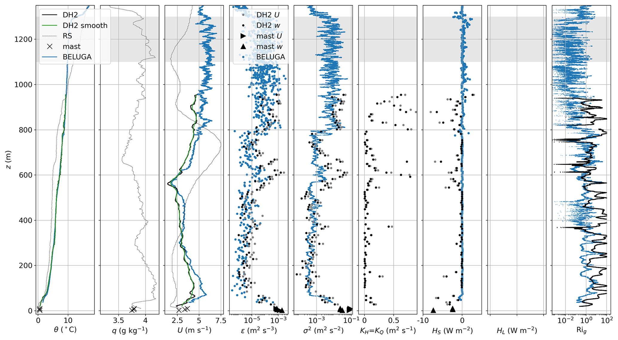
Figure 10Vertical profiles for 13 July (first descent). Panels are as in Fig. 9, but no reliable q and HL data from the DH2 are available for this case.
Dissipation rates and wind speed variances again show a similar turbulent structure and define the cloud-driven mixed layer with increased turbulence inside and below the cloud between 800 and 1300 m. Observations of vertical velocity and spectral width from the cloud radar (not shown) also support this general structure. This mixing is caused by cloud-top radiative cooling, which drives buoyant, upside-down shallow convection extending below cloud base. Due to relatively weak turbulence, the cloud-driven mixed layer does not extend below about 800 m, such that this layer is decoupled from lower atmospheric layers and the surface below. Below the mixed layer, turbulence is very weak; thus, this stable layer decouples the mixed layer from the surface. At around 600 m, another thin layer of increased turbulence (more pronounced in DH2 data than for BELUGA) seems to be associated with an intermittent and thin secondary cloud layer occasionally visible at different levels below the primary cloud in the radar data (Fig. 1). At the bottom, the surface-driven turbulent layer extends up to about 75 m within the surface-based temperature inversion. The profile of turbulent exchange coefficients K shows increased values where turbulence is highest: close to the surface, within the cloud-driven mixed layer and at the secondary cloud layer near 600 m, leading to negative (downward) sensible heat fluxes in these layers. DH2 flux estimates fluctuate much more than BELUGA flux estimates, probably due to the longer averaging times for BELUGA. The negative sensible heat fluxes at around 800 m are basically a detrainment of heat from the cloud-driven mixed layer. The mixed layer is relatively warm (θ≈10 ∘C) and probably had little interaction with the melting sea ice surface (at ∼0 ∘C) over the course of its advective path. This is similarly described in Shupe et al. (2013): a relatively warm, moist air mass moves over the sea ice and remains decoupled from the surface partly because of the vast difference in the thermodynamic state of the cloudy mixed layer versus the surface layer. Some of the warmth of the layer is lost due to radiative cooling at the cloud top, and some is lost by downward mixing, which effectively increases the energy content of the layer between 0 and 800 m and also contributes to sensible heating of the surface, as seen in the surface layer. The magnitude of DH2 near-surface fluxes agrees well with tower-derived fluxes, despite the disparity in averaging intervals. However, even the relatively reliable tower estimates differ by 5 W m−2 between the individual measurement heights, which suggests strong variability in the surface layer. Altogether, the observations of ABL conditions with a decoupled, cloud-driven mixed layer are in agreement with previous observations (Shupe et al., 2013; Sotiropoulou et al., 2014) and add information about downward turbulent fluxes at layer interfaces.
3.3 The 9 April 2020: cloud- and wind-shear-driven turbulence
The 9 April 2020 is a case with a mixed-phase cloud typical of the Arctic ABL. At the time of the DH2 flight, radar and lidar data show a persistent liquid cloud with cloud base at about 900 m and ice crystal precipitation (and sublimation) below (Fig. 1). The radar Doppler spectral width shows turbulent mixing as a result of cloud radiative cooling and buoyancy extending below the cloud base down to approximately 500 m (not shown). The DH2 flew a vertical profile up to just below cloud base at 900 m, but no BELUGA flights are available. Figure 11 depicts the rather complicated ABL structure recorded by the DH2. The thin (100 m thick), near-neutral surface layer is capped by stable stratification above with several smaller temperature inversions between the surface and 600 m, some weak overturning at 500 m, and slightly stable to near-neutral conditions above 600 m. Throughout, temperatures are very low: down to −22 ∘C at the surface and −14 ∘C near the cloud base. The specific humidity profile resembles the temperature profile; the liquid water content is very low due to the cold temperatures. The profile reveals an apparent moisture inversion above the surface to 300 m, highlighting the important role of advective moisture (and the limited surface source of moisture at this time of the year). The wind profile exhibits a weak LLJ in the stably stratified region between the surface and 600 m with a maximum wind speed of 7.5 m s−1 at 400 m.
The turbulence profiles for ε and feature several turbulence maxima probably generated from three different sources: (i) surface-based turbulence – the vertical profiles seem to clearly continue the mast measurements, (ii) cloud-driven turbulence evident as a constant turbulence magnitude between cloud base and the lower boundary of the near-neutral layer at 500 m, and (iii) shear-induced turbulence by the LLJ with a local minimum at the jet core and increased values below and above at 300 and 500 m, respectively. An increase in turbulent dissipation on the upper and lower edges of the LLJ has been observed in previous studies relating LLJs to turbulence (e.g., Banta et al., 2006; Smedman et al., 1993). Throughout the profile, the turbulence is strongest at the interface of the cloud mixed layer with the upper bound of the LLJ at 500 m, where the temperature profile also shows overturning. At this altitude, the turbulent heat fluxes are also most pronounced, with a negative (downward) sensible and latent heat flux at the top of the temperature and humidity inversion. The variability in HS at the bottom of the cloud-driven mixed layer reflects the slight variation in θ between 500 and 600 m. Probably, the base of the mixed layer is not static but varies in space and time, leading to some inconsistencies and turbulent exchanges. The presence of some upward sensible heat fluxes above suggests the interaction of multiple layers in that zone (also subtly seen in the temperature profile). Comparison with the radiosonde suggests that there is an evolution in this layer just above 500 m. Downward-oriented heat fluxes also occur just below the jet core, and a stronger upward-directed flux (15 W m−2) is observed in the near-neutral surface layer. Lastly, the Rig profile again shows very small values in the high-turbulence regions.
For all three cases presented here, the observations represent typical ABL structures in the Arctic that have been observed previously. The DH2 observations add valuable information about the turbulence vertical structure and turbulent fluxes in regions with pronounced turbulence. Although flux magnitudes seem to be consistent with surface flux measurements, the absolute values of fluxes should be treated with caution, as the variance estimates only include small scales due to the short time records. Nonetheless, the method presented provides a robust idea of the vertical profile shape of turbulent fluxes.
This work and the case studies herein demonstrate the potential of DH2 measurements to analyze turbulence and turbulent fluxes in the Arctic ABL as observed during MOSAiC. The flux gradient method with the parameterization of the turbulent exchange coefficient is an established method to derive vertical profiles of turbulent fluxes. The method of Hanna (1968) has been applied with sUAS measurements before by Platis et al. (2016) for studying particle fluxes by means of Km. The present study extends the Hanna (1968) method to KH and KQ for sensible and latent heat fluxes by parameterizing the relation of different turbulent exchange coefficients via Prt. For this, we apply a parameterization of Prt depending on stability derived from airborne measurements in the Arctic ABL (Aliabadi et al., 2016). If the flux method is applied to DH2 measurements in other locations, the selection of the Prt parameterization might have to be re-evaluated depending on prevailing stability conditions. Another novelty presented here is an empirical description of anisotropy in the vertical ABL profile depending on the gradient Richardson number as a stability parameter. With this relation, fluctuations in vertical wind components can be inferred from measurements of the horizontal component. The anisotropy relation was derived from airborne sonic anemometer measurements during MOSAiC and another Arctic field campaign. As a result, the extended flux method allows one to estimate vertical profiles of turbulent fluxes based on measurements of the one-dimensional, high-resolution horizontal wind speed along with a low-resolution temperature/humidity measurement. Hence, measurement instrumentation can be kept relatively simple, which is advantageous with the limited payload and battery capacity of sUASs.
However, the applied method is subject to several limitations. Generally, the flux gradient method is more suitable for stable stratification (which mostly applies to conditions in this study) than for unstable conditions, and counter-gradient fluxes are not represented by the method. However, studying stable ABLs brings different challenges: with shallow vertical gradients and small flux magnitudes, small perturbations in the measured parameters increase relative flux errors. Moreover, the length scales and timescales included in the flux estimates are restricted by the averaging time for variances (Eq. 4 and the empirical anisotropy description) because the flux magnitude is proportional to the square of variances (when assuming correctly estimated dissipation rates). The estimates for variances include only timescales smaller than the averaging time, so the derived fluxes represent the small-scale turbulent transport, and may underestimate the total flux. Further, short averaging intervals, compared with integral timescales, increase random and systematic errors of variances and fluxes (Lenschow et al., 1994). Nonetheless, DH2 flux magnitudes near the surface agree well with eddy covariance fluxes from a co-located ground-based tower. Other limitations result from the measurement mode typical of sUASs. First, the DH2 helix flight pattern produces a slant profile instead of a true vertical profile. We assume the slant profile measurements as horizontal and average these over a certain height interval. If the interval is too small, horizontal heterogeneity might appear as “vertical” fluctuations (Balsley et al., 2018). On the other hand, the interval cannot be too long or the method will not achieve the desired vertical resolution. Second, most DH2 flights are located outside of clouds, and the flights are limited to lower-wind conditions, which excludes some case analyses that might be especially interesting when studying the Arctic ABL. Further errors might occur due to DH2-specific issues and the measurement conditions: the wind estimation is inaccurate under certain conditions of extreme flight dynamics (de Boer et al., 2022; Doddi et al., 2022) and the wake of the ship during MOSAiC might have influenced the measurements near the surface. Lastly, the empirical anisotropy relation relies on relatively few BELUGA measurements in stable stratification. For future applications, the authors recommend extending and verifying this relation.
Despite all these limitations, the DH2 results agree well with established measurement methods like meteorological flux towers and radar. This provides confidence in the obtained results and offers the following novel insights into turbulent transport processes in the Arctic ABL:
- i.
The case studies in this work represent typical Arctic ABL structures observed in previous studies. Nonetheless, high-resolution vertical profile measurements are rare, and the DH2 may offer very detailed insights into turbulent exchange processes.
- ii.
These vertical profile details also provide important context for the evolution of the surface energy budget, which then controls the sea ice thermodynamic state and melt. In particular, this is evident in the 13 July case where downward sensible heat fluxes warm the near-surface layer and support ice melt.
- iii.
In the past, these vertical transfers of turbulent heat fluxes within the ABL have typically been inferred from model simulations, as very few measurements were available of this type. The results from the presented method will be essential for evaluating LES studies examining the energy and moisture budgets associated with clouds and cloud-driven mixed layers (e.g., Solomon et al., 2014; Neggers et al., 2019).
The methods shown in this study will be extended to further cases of interest, which requires careful examination of the available measurements for each individual case. Turbulent flux profiles from the DH2 are available from a wide operation period during MOSAiC, from winter to the melt season. The resulting vertical profiles of turbulent fluxes can be analyzed concerning different ABL and sea ice conditions, including the influence of atmospheric stability, stratification, clouds, leads, and melt ponds to understand the complex interactions between ABL processes, the surface energy budget, and sea ice. Some of these cases can support LES studies, where these new observation-based perspectives will add unique new constraints on cloud, turbulence, and moisture processes. All of these insights will help to advance our understanding of how turbulent fluxes influence the interactions between the Arctic atmosphere and surface.
DataHawk2 meteorological data are available from the Arctic Data Center: https://doi.org/10.18739/A22Z12Q8X (Jozef et al., 2021) and https://doi.org/10.18739/A2Z31NQ11 (Jozef et al., 2022b). BELUGA turbulence data during MOSAiC are hosted on PANGAEA: https://doi.org/10.1594/PANGAEA.931404 (Egerer et al., 2021b). Met tower data are available from the Arctic Data Center: https://doi.org/10.18739/A2VM42Z5F (Cox et al., 2021). Cloud Radar data are available from the DOE ARM archive: https://doi.org/10.5439/1393437 (Johnson et al., 2021). BELUGA turbulence data during PASCAL are hosted on PANGAEA: https://doi.org/10.1594/PANGAEA.899803 (Egerer et al., 2019b).
UE performed the turbulence data analysis with support from DL and AD. GJ, GdB, JJC, RC, and JH conducted the DataHawk2 flights and post-processed and published the meteorological data. DL developed the DH2 platform and turbulence sensors. MDS was the ATMOS team lead during MOSAiC and complemented the case descriptions with additional ground-based data. CP and ML collected the BELUGA data during MOSAiC, and HS was the BELUGA PI during MOSAiC. UE compiled the manuscript with contributions from all co-authors.
The contact author has declared that none of the authors has any competing interests.
Publisher’s note: Copernicus Publications remains neutral with regard to jurisdictional claims in published maps and institutional affiliations.
This work was supported by the CIRES Visiting Fellows Program that is funded by the NOAA Cooperative Agreement with CIRES, NA17OAR4320101. Data used in this paper were produced as part of the international Multidisciplinary drifting Observatory for the Study of Arctic Climate (MOSAiC) with the tag MOSAiC20192020. We thank everyone involved in the RV Polarstern expedition during MOSAiC in 2019–2020 (project no. AWI_PS122_00), as listed in Nixdorf et al. (2021). Matthew D. Shupe was supported by the US National Science Foundation (grant no. OPP-1734551), the DOE Atmospheric System Research program (grant nos. DE-SC00021341 and DE-SC0023036), and the NOAA Physical Sciences Laboratory (grant no. NA22OAR4320151). Gijs de Boer was supported by the US National Science Foundation Office of Polar Programs (grant no. OPP 1805569), the US Department of Energy Atmospheric Systems Research program (grant no. DE-SC0013306), and the NOAA Physical Sciences Laboratory. Dale Lawrence was supported by the US National Science Foundation (grant nos. PDM-2128444 and OPP-1805569). Abhiram Doddi was supported by the US National Science Foundation (grant no. PDM-2128444). Part of the work was supported by the Deutsche Forschungsgemeinschaft (German Research Foundation; project no. 268020496–TRR 172) within sub-project A02 of the Transregional Collaborative Research Center “ArctiC Amplification: Climate Relevant Atmospheric and SurfaCe Processes, and Feedback Mechanisms (AC)3” project. A subset of data was obtained from the Atmospheric Radiation Measurement (ARM) User Facility, a US Department of Energy (DOE) Office of Science user facility managed by the Biological and Environmental Research program. The authors would like to thank Andrey Grachev and Chris Fairall for fruitful discussions.
This research has been supported by the CIRES Visiting Fellows Program that is funded by the NOAA Cooperative Agreement with CIRES (grant no. NA17OAR4320101).
This paper was edited by Cléo Quaresma Dias-Junior and reviewed by Sean Bailey and one anonymous referee.
Abarbanel, H. D. I., Holm, D. D., Marsden, J. E., and Ratiu, T.: Richardson Number Criterion for the Nonlinear Stability of Three-Dimensional Stratified Flow, Phys. Rev. Lett., 52, 2352–2355, https://doi.org/10.1103/PhysRevLett.52.2352, 1984. a
Aliabadi, A. A., Staebler, R., Liu, M., and Herber, A.: Characterization and Parametrization of Reynolds Stress and Turbulent Heat Flux in the Stably-Stratified Lower Arctic Troposphere Using Aircraft Measurements, Bound.-Lay. Meteorol., 161, 99–126, https://doi.org/10.1007/s10546-016-0164-7, 2016. a, b, c, d
Balsley, B. B., Lawrence, D. A., Fritts, D. C., Wang, L., Wan, K., and Werne, J.: Fine Structure, Instabilities, and Turbulence in the Lower Atmosphere: High-Resolution In Situ Slant-Path Measurements with the DataHawk UAV and Comparisons with Numerical Modeling, J. Atmos. Ocean. Tech., 35, 619–642, https://doi.org/10.1175/JTECH-D-16-0037.1, 2018. a, b, c, d, e
Bange, J. and Roth, R.: Helicopter-borne flux measurements in the nocturnal boundary layer over land – a case study, Bound.-Lay. Meteorol., 92, 295–325, https://doi.org/10.1023/A:1002078712313, 1999. a
Banta, R. M., Pichugina, Y. L., and Brewer, W. A.: Turbulent Velocity-Variance Profiles in the Stable Boundary Layer Generated by a Nocturnal Low-Level Jet, J. Atmos. Sci., 63, 2700–2719, https://doi.org/10.1175/JAS3776.1, 2006. a
Bhumralkar, C. M.: Parameterization of the planetary boundary layer in atmospheric general circulation models, Rev. Geophys., 14, 215–226, https://doi.org/10.1029/RG014i002p00215, 1976. a
Biltoft, C. A.: Some thoughts on local isotropy and the lateral to longitudinal velocity spectrum ratio, Bound.-Lay. Meteorol., 100, 393–404, 2001. a
Båserud, L., Reuder, J., Jonassen, M. O., Bonin, T. A., Chilson, P. B., Jiménez, M. A., and Durand, P.: Potential and Limitations in Estimating Sensible-Heat-Flux Profiles from Consecutive Temperature Profiles Using Remotely-Piloted Aircraft Systems, Bound.-Lay. Meteorol., 174, 145–177, https://doi.org/10.1007/s10546-019-00478-9, 2019. a
Busch, N. E. and Panofsky, H. A.: Recent spectra of atmospheric turbulence, Q. J. Roy. Meteor. Soc., 94, 132–148, https://doi.org/10.1002/qj.49709440003, 1968. a
Bélair, S., Mailhot, J., Strapp, J. W., and MacPherson, J.I.: An Examination of Local versus Nonlocal Aspects of a TKE-Based Boundary Layer Scheme in Clear Convective Conditions, J. Appl. Meteorol., 38, 1499–1518, https://doi.org/10.1175/1520-0450(1999)038<1499:AEOLVN>2.0.CO;2, 1999. a
Calmer, R., Roberts, G. C., Preissler, J., Sanchez, K. J., Derrien, S., and O'Dowd, C.: Vertical wind velocity measurements using a five-hole probe with remotely piloted aircraft to study aerosol–cloud interactions, Atmos. Meas. Tech., 11, 2583–2599, https://doi.org/10.5194/amt-11-2583-2018, 2018. a
Cox, C., Gallagher, M., Shupe, M., Persson, O., Solomon, A., Blomquist, B., Brooks, I., Costa, D., Gottas, D., Hutchings, J., Osborn, J., Morris, S., Preusser, A., and Uttal, T.: 10-meter meteorological flux tower measurements (Level 1 Raw), Multidisciplinary Drifting Observatory for the Study of Arctic Climate (MOSAiC), central Arctic, October 2019 - September 2020, Arctic Data Center [data set], https://doi.org/10.18739/A2VM42Z5F, 2021. a, b, c
Cuxart, J., Holtslag, A. A., Beare, R. J., Bazile, E., Beljaars, A., Cheng, A., Conangla, L., Ek, M., Freedman, F., Hamdi, R., Kerstein, A., Kitagawa, H., Lenderink, G., Lewellen, D., Mailhot, J., Mauritsen, T., Perov, V., Schayes, G., Steeneveld, G. J., Svensson, G., Taylor, P., Weng, W., Wunsch, S., and Xu, K. M.: Single-column model intercomparison for a stably stratified atmospheric boundary layer, Bound.-Lay. Meteorol., 118, 273–303, https://doi.org/10.1007/s10546-005-3780-1, 2006. a
de Boer, G., Ivey, M., Schmid, B., Lawrence, D., Dexheimer, D., Mei, F., Hubbe, J., Bendure, A., Hardesty, J., Shupe, M. D., McComiskey, A., Telg, H., Schmitt, C., Matrosov, S. Y., Brooks, I., Creamean, J., Solomon, A., Turner, D. D., Williams, C., Maahn, M., Argrow, B., Palo, S., Long, C. N., Gao, R.-S., and Mather, J.: A Bird's-Eye View: Development of an Operational ARM Unmanned Aerial Capability for Atmospheric Research in Arctic Alaska, B. Am. Meteorol. Soc., 99, 1197–1212, https://doi.org/10.1175/BAMS-D-17-0156.1, 2018. a
de Boer, G., Calmer, R., Jozef, G., Cassano, J. J., Hamilton, J., Lawrence, D., Borenstein, S., Doddi, A., Cox, C., Schmale, J., Preußer, A., and Argrow, B.: Observing the Central Arctic Atmosphere and Surface with University of Colorado uncrewed aircraft systems, Scientific Data, 9, 439, https://doi.org/10.1038/s41597-022-01526-9, 2022. a, b, c, d
Doddi, A.: Insitu Sensing and Analysis of Turbulence - Investigation to Enhance Fine-Structure Turbulence Observation Capabilities of Autonomous Aircraft Systems, dissertation, CU Boulder, https://scholar.colorado.edu/concern/graduate_thesis_or_dissertations/kp78gh76n (last access: 21 April 2023), 2021. a
Doddi, A., Lawrence, D., Fritts, D., Wang, L., Lund, T., Brown, W., Zajic, D., and Kantha, L.: Instabilities, Dynamics, and Energetics accompanying Atmospheric Layering (IDEAL): high-resolution in situ observations and modeling in and above the nocturnal boundary layer, Atmos. Meas. Tech., 15, 4023–4045, https://doi.org/10.5194/amt-15-4023-2022, 2022. a, b, c, d
Dyer, A. J.: The turbulent transport of heat and water vapour in an unstable atmosphere, Q. J. Roy. Meteor. Soc., 93, 501–508, https://doi.org/10.1002/qj.49709339809, 1967. a
Egerer, U., Gottschalk, M., Siebert, H., Ehrlich, A., and Wendisch, M.: The new BELUGA setup for collocated turbulence and radiation measurements using a tethered balloon: first applications in the cloudy Arctic boundary layer, Atmos. Meas. Tech., 12, 4019–4038, https://doi.org/10.5194/amt-12-4019-2019, 2019a. a, b, c, d, e, f
Egerer, U., Gottschalk, M., Siebert, H., Wendisch, M., and Ehrlich, A.: Tethered balloon-borne measurements of turbulence and radiation during the Arctic field campaign PASCAL in June 2017, PANGAEA [data set], https://doi.org/10.1594/PANGAEA.899803, 2019b. a
Egerer, U., Ehrlich, A., Gottschalk, M., Griesche, H., Neggers, R. A. J., Siebert, H., and Wendisch, M.: Case study of a humidity layer above Arctic stratocumulus and potential turbulent coupling with the cloud top, Atmos. Chem. Phys., 21, 6347–6364, https://doi.org/10.5194/acp-21-6347-2021, 2021a. a, b, c
Egerer, U., Pilz, C., Lonardi, M., Siebert, H., and Wendisch, M.: Tethered balloon-borne measurements of turbulence during MOSAiC leg 4 in July 2020, PANGAEA [data set], https://doi.org/10.1594/PANGAEA.931404, 2021b. a
Frehlich, R., Meillier, Y., Jensen, M. L., and Balsley, B.: Turbulence Measurements with the CIRES Tethered Lifting System during CASES-99: Calibration and Spectral Analysis of Temperature and Velocity, J. Atmos. Sci., 60, 2487–2495, https://doi.org/10.1175/1520-0469(2003)060<2487:TMWTCT>2.0.CO;2, 2003. a, b
Galperin, B., Sukoriansky, S., and Anderson, P. S.: On the critical Richardson number in stably stratified turbulence, Atmos. Sci. Lett., 8, 65–69, https://doi.org/10.1002/asl.153, 2007. a, b
Grachev, A. A., Andreas, E. L., Fairall, C. W., Guest, P. S., and Persson, P. O. G.: On the turbulent Prandtl number in the stable atmospheric boundary layer, Bound.-Lay. Meteorol., 125, 329–341, https://doi.org/10.1007/s10546-007-9192-7, 2007. a, b, c, d
Greene, B. R., Kral, S. T., Chilson, P. B., and Reuder, J.: Gradient-Based Turbulence Estimates from Multicopter Profiles in the Arctic Stable Boundary Layer, Bound.-Lay. Meteorol., 183, 321–353, https://doi.org/10.1007/s10546-022-00693-x, 2022. a
Hamilton, J., de Boer, G., Doddi, A., and Lawrence, D. A.: The DataHawk2 uncrewed aircraft system for atmospheric research, Atmos. Meas. Tech., 15, 6789–6806, https://doi.org/10.5194/amt-15-6789-2022, 2022. a, b, c
Hanna, S. R.: A model of vertical turbulent transport in the atmosphere, dissertation, The Pennsylvania State University, 1967. a
Hanna, S. R.: A Method of Estimating Vertical Eddy Transport in the Planetary Boundary Layer Using Characteristics of the Vertical Velocity Spectrum, J. Atmos. Sci., 25, 1026–1033, https://doi.org/10.1175/1520-0469(1968)025<1026:AMOEVE>2.0.CO;2, 1968. a, b, c, d, e, f, g, h
He, J., Chan, P., Li, Q., Li, L., Zhang, L., and Yang, H.: Observation of vertical eddy diffusivity and mixing length during landfalling Super Typhoons, J. Wind Eng. Ind. Aerod., 219, 104816, https://doi.org/10.1016/j.jweia.2021.104816, 2021. a
Hinze, J.: Turbulence, McGraw-Hill, New York, ISBN 0070290377, 1975. a
Holt, T. and Raman, S.: A review and comparative evaluation of multilevel boundary layer parameterizations for first-order and turbulent kinetic energy closure schemes, Rev. Geophys., 26, 761–780, https://doi.org/10.1029/RG026i004p00761, 1988. a
Howell, J. F. and Sun, J.: Surface-layer fluxes in stable conditions, Bound.-Lay. Meteorol., 90, 495–520, https://doi.org/10.1023/A:1001788515355, 1999. a
Högström, U., Hunt, J. C., and Smedman, A. S.: Theory and measurements for turbulence spectra and variances in the atmospheric neutral surface layer, Bound.-Lay. Meteorol., 103, 101–124, https://doi.org/10.1023/A:1014579828712, 2002. a
Johnson, K., Giangrande, S., and Toto, T.: Active Remote Sensing of Cloud Layers (ARSCL) Product using Ka-Band ARM Zenith Radars (ARSCLKAZR1KOLLIAS), ARM [data set], https://doi.org/10.5439/1393437, 2021. a, b, c, d
Jonassen, M. O., Tisler, P., Altstädter, B., Scholtz, A., Vihma, T., Lampert, A., König-Langlo, G., and Lüpkes, C.: Application of remotely piloted aircraft systems in observing the atmospheric boundary layer over Antarctic sea ice in winter, Polar Res., 34, 25651, https://doi.org/10.3402/polar.v34.25651, 2015. a
Jozef, G., de Boer, G., Cassano, J., Calmer, R., Hamilton, J., Lawrence, D., Borenstein, S., Doddi, A., Schmale, J., Preußer, A., and Argrow, B.: DataHawk2 Uncrewed Aircraft System data from the Multidisciplinary drifting Observatory for the Study of Arctic Climate (MOSAiC) campaign, A1 level, Arctic Data Center [data set], https://doi.org/10.18739/A22Z12Q8X, 2021. a, b
Jozef, G., Cassano, J., Dahlke, S., and de Boer, G.: Testing the efficacy of atmospheric boundary layer height detection algorithms using uncrewed aircraft system data from MOSAiC, Atmos. Meas. Tech., 15, 4001–4022, https://doi.org/10.5194/amt-15-4001-2022, 2022a. a, b
Jozef, G., de Boer, G., Cassano, J., Calmer, R., Hamilton, J., Lawrence, D., Borenstein, S., Doddi, A., Schmale, J., Preußer, A., and Argrow, B.: DataHawk2 Uncrewed Aircraft System data from the Multidisciplinary drifting Observatory for the Study of Arctic Climate (MOSAiC) campaign, raw data, Arctic Data Center [data set], https://doi.org/10.18739/A2Z31NQ11, 2022b. a, b
Kantha, L., Lawrence, D., Luce, H., Hashiguchi, H., Tsuda, T., Wilson, R., Mixa, T., and Yabuki, M.: Shigaraki UAV-Radar Experiment (ShUREX): overview of the campaign with some preliminary results, Progress in Earth and Planetary Science, 4, 19, https://doi.org/10.1186/s40645-017-0133-x, 2017. a
Kim, J. and Mahrt, L.: Simple formulation of turbulent mixing in the stable free atmosphere and nocturnal boundary layer, Tellus A, 44, 381–394, https://doi.org/10.3402/tellusa.v44i5.14969, 1992. a
Knust, R.: Polar research and supply vessel POLARSTERN operated by the Alfred-Wegener-Institute, Journal of large-scale research facilities, 3, A119, https://doi.org/10.17815/jlsrf-3-163, 2017. a
Knuth, S. L. and Cassano, J. J.: Estimating Sensible and Latent Heat Fluxes Using the Integral Method from in situ Aircraft Measurements, J. Atmos. Ocean. Tech., 31, 1964–1981, https://doi.org/10.1175/JTECH-D-14-00008.1, 2014. a
Kolmogorov, A. N.: Dissipation of Energy in Locally Isotropic Turbulence, Dokl. Akad. Nauk SSSR+, 32, 16 pp., 1941. a, b
Kondo, J., Kanechika, O., and Yasuda, N.: Heat and Momentum Transfers under Strong Stability in the Atmospheric Surface Layer, J. Atmos. Sci., 35, 1012–1021, https://doi.org/10.1175/1520-0469(1978)035<1012:HAMTUS>2.0.CO;2, 1978. a, b
Kral, S. T., Reuder, J., Vihma, T., Suomi, I., Haualand, K. F., Urbancic, G. H., Greene, B. R., Steeneveld, G.-J., Lorenz, T., Maronga, B., Jonassen, M. O., Ajosenpää, H., Båserud, L., Chilson, P. B., Holtslag, A. A. M., Jenkins, A. D., Kouznetsov, R., Mayer, S., Pillar-Little, E. A., Rautenberg, A., Schwenkel, J., Seidl, A. W., and Wrenger, B.: The Innovative Strategies for Observations in the Arctic Atmospheric Boundary Layer Project (ISOBAR) – Unique fine-scale observations under stable and very stable conditions, B. Am. Meteorol. Soc., 102, E218–E243, https://doi.org/10.1175/BAMS-D-19-0212.1, 2020. a, b
Lampert, A., Altstädter, B., Bärfuss, K., Bretschneider, L., Sandgaard, J., Michaelis, J., Lobitz, L., Asmussen, M., Damm, E., Käthner, R., Krüger, T., Lüpkes, C., Nowak, S., Peuker, A., Rausch, T., Reiser, F., Scholtz, A., Sotomayor Zakharov, D., Gaus, D., Bansmer, S., Wehner, B., and Pätzold, F.: Unmanned Aerial Systems for Investigating the Polar Atmospheric Boundary Layer—Technical Challenges and Examples of Applications, Atmosphere, 11, 416, https://doi.org/10.3390/atmos11040416, 2020. a
Lawrence, D. A. and Balsley, B. B.: High-Resolution Atmospheric Sensing of Multiple Atmospheric Variables Using the DataHawk Small Airborne Measurement System, J. Atmos. Ocean. Tech., 30, 2352–2366, https://doi.org/10.1175/JTECH-D-12-00089.1, 2013. a
Lee, X.: Turbulence Spectra and Eddy Diffusivity over Forests, J. Appl. Meteorol. Clim., 35, 1307–1318, https://doi.org/10.1175/1520-0450(1996)035<1307:TSAEDO>2.0.CO;2, 1996. a
Lenschow, D. H., Mann, J., and Kristensen, L.: How Long Is Long Enough When Measuring Fluxes and Other Turbulence Statistics?, J. Atmos. Ocean. Tech., 11, 661–673, https://doi.org/10.1175/1520-0426(1994)011<0661:HLILEW>2.0.CO;2, 1994. a
Li, D.: Turbulent Prandtl number in the atmospheric boundary layer – where are we now?, Atmos. Res., 216, 86–105, https://doi.org/10.1016/j.atmosres.2018.09.015, 2019. a, b, c
Lonardi, M., Pilz, C., Akansu, E. F., Dahlke, S., Egerer, U., Ehrlich, A., Griesche, H., Heymsfield, A. J., Kirbus, B., Schmitt, C. G., Shupe, M. D., Siebert, H., Wehner, B., and Wendisch, M.: Tethered balloon-borne profile measurements of atmospheric properties in the cloudy atmospheric boundary layer over the Arctic sea ice during MOSAiC: Overview and first results, Elementa: Science of the Anthropocene, 10, 000120, https://doi.org/10.1525/elementa.2021.000120, 2022. a, b, c, d, e, f
Lovejoy, S., Tuck, A. F., Hovde, S. J., and Schertzer, D.: Is isotropic turbulence relevant in the atmosphere?, Geophys. Res. Lett., 34, L15802, https://doi.org/10.1029/2007GL029359, 2007. a
Luce, H., Kantha, L., Hashiguchi, H., Lawrence, D., and Doddi, A.: Turbulence kinetic energy dissipation rates estimated from concurrent UAV and MU radar measurements, Earth Planets Space, 70, 207, https://doi.org/10.1186/s40623-018-0979-1, 2018. a, b
Luce, H., Kantha, L., Hashiguchi, H., and Lawrence, D.: Estimation of Turbulence Parameters in the Lower Troposphere from ShUREX (2016–2017) UAV Data, Atmosphere, 10, 384, https://doi.org/10.3390/atmos10070384, 2019. a, b, c, d, e
Mack, S. A. and Schoeberlein, H. C.: Richardson Number and Ocean Mixing: Towed Chain Observations, J. Phys. Oceanogr., 34, 736–754, https://doi.org/10.1175/1520-0485(2004)034<0736:RNAOMT>2.0.CO;2, 2004. a
Mahrt, L. and Vickers, D.: Formulation of Turbulent Fluxes in the Stable Boundary Layer, J. Atmos. Sci., 60, 2538–2548, https://doi.org/10.1175/1520-0469(2003)060<2538:FOTFIT>2.0.CO;2, 2003. a
Mauritsen, T. and Svensson, G.: Observations of Stably Stratified Shear-Driven Atmospheric Turbulence at Low and High Richardson Numbers, J. Atmos. Sci., 64, 645–655, https://doi.org/10.1175/JAS3856.1, 2007. a, b
McNider, R. T. and Pour-Biazar, A.: Meteorological modeling relevant to mesoscale and regional air quality applications: a review, J. Air Waste Manage., 70, 2–43, https://doi.org/10.1080/10962247.2019.1694602, 2020. a
Miles, J. W.: On the stability of heterogeneous shear flows, J. Fluid Mech., 10, 496–508, https://doi.org/10.1017/S0022112061000305, 1961. a
Monti, P., Fernando, H. J. S., Princevac, M., Chan, W. C., Kowalewski, T. A., and Pardyjak, E. R.: Observations of Flow and Turbulence in the Nocturnal Boundary Layer over a Slope, J. Atmos. Sci., 59, 2513–2534, https://doi.org/10.1175/1520-0469(2002)059<2513:OOFATI>2.0.CO;2, 2002. a
Muschinski, A., Frehlich, R. G., and Balsley, B. B.: Small-scale and large-scale intermittency in the nocturnal boundary layer and the residual layer, J. Fluid Mech., 515, 319–351, https://doi.org/10.1017/S0022112004000412, 2004. a
Neggers, R. A. J., Chylik, J., Egerer, U., Griesche, H., Schemann, V., Seifert, P., Siebert, H., and Macke, A.: Local and Remote Controls on Arctic Mixed-Layer Evolution, J. Adv. Model. Earth Sy., 11, 2214–2237, https://doi.org/10.1029/2019MS001671, 2019. a
Nieuwstadt, F. T. M.: The turbulent structure of the stable nocturnal boundary layer, J. Atmos. Sci., 41, 2202–2216, 1984. a
Nixdorf, U., Dethloff, K., Rex, M., Shupe, M., Sommerfeld, A., Perovich, D. K., Nicolaus, M., Heuzé, C., Rabe, B., Loose, B., Damm, E., Gradinger, R., Fong, A., Maslowski, W., Rinke, A., Kwok, R., Spreen, G., Wendisch, M., Herber, A., Hirsekorn, M., Mohaupt, V., Frickenhaus, S., Immerz, A., Weiss-Tuider, K., König, B., Mengedoht, D., Regnery, J., Gerchow, P., Ransby, D., Krumpen, T., Morgenstern, A., Haas, C., Kanzow, T., Rack, F. R., Saitzev, V., Sokolov, V., Makarov, A., Schwarze, S., Wunderlich, T., Wurr, K., and Boetius, A.: MOSAiC Extended Acknowledgement, Version 2, Zenodo, https://doi.org/10.5281/zenodo.5541624, 2021. a
Nowak, J. L., Siebert, H., Szodry, K.-E., and Malinowski, S. P.: Coupled and decoupled stratocumulus-topped boundary layers: turbulence properties, Atmos. Chem. Phys., 21, 10965–10991, https://doi.org/10.5194/acp-21-10965-2021, 2021. a
Panofsky, H. A., Blackadar, A. K., and McVehil, G. E.: The diabatic wind profile, Q. J. Roy. Meteor. Society, 86, 390–398, https://doi.org/10.1002/qj.49708636911, 1960. a
Platis, A., Altstädter, B., Wehner, B., Wildmann, N., Lampert, A., Hermann, M., Birmili, W., and Bange, J.: An Observational Case Study on the Influence of Atmospheric Boundary-Layer Dynamics on New Particle Formation, Bound.-Lay. Meteorol., 158, 67–92, https://doi.org/10.1007/s10546-015-0084-y, 2016. a, b
Pope, S. B.: Turbulent Flows, Cambridge University Press, https://doi.org/10.1017/CBO9780511840531, 2000. a, b
Rautenberg, A., Allgeier, J., Jung, S., and Bange, J.: Calibration Procedure and Accuracy of Wind and Turbulence Measurements with Five-Hole Probes on Fixed-Wing Unmanned Aircraft in the Atmospheric Boundary Layer and Wind Turbine Wakes, Atmosphere, 10, 124, https://doi.org/10.3390/atmos10030124, 2019. a
Rinke, A., Cassano, J. J., Cassano, E. N., Jaiser, R., and Handorf, D.: Meteorological conditions during the MOSAiC expedition: Normal or anomalous?, Elementa: Science of the Anthropocene, 9, 00023, https://doi.org/10.1525/elementa.2021.00023, 00023, 2021. a
Schmithüsen, H.: Continuous meteorological surface measurement during POLARSTERN cruise PS122/3, PANGAEA [data set], https://doi.org/10.1594/PANGAEA.935223, 2021. a, b
Schumann, U. and Gerz, T.: Turbulent Mixing in Stably Stratified Shear Flows, J. Appl. Meteorol. Clim., 34, 33–48, https://doi.org/10.1175/1520-0450-34.1.33, 1995. a
Shupe, M. D., Persson, P. O. G., Brooks, I. M., Tjernström, M., Sedlar, J., Mauritsen, T., Sjogren, S., and Leck, C.: Cloud and boundary layer interactions over the Arctic sea ice in late summer, Atmos. Chem. Phys., 13, 9379–9399, https://doi.org/10.5194/acp-13-9379-2013, 2013. a, b
Shupe, M. D., Rex, M., Blomquist, B., Persson, P. O. G., Schmale, J., Uttal, T., Althausen, D., Angot, H., Archer, S., Bariteau, L., Beck, I., Bilberry, J., Bucci, S., Buck, C., Boyer, M., Brasseur, Z., Brooks, I. M., Calmer, R., Cassano, J., Castro, V., Chu, D., Costa, D., Cox, C. J., Creamean, J., Crewell, S., Dahlke, S., Damm, E., de Boer, G., Deckelmann, H., Dethloff, K., Dütsch, M., Ebell, K., Ehrlich, A., Ellis, J., Engelmann, R., Fong, A. A., Frey, M. M., Gallagher, M. R., Ganzeveld, L., Gradinger, R., Graeser, J., Greenamyer, V., Griesche, H., Griffiths, S., Hamilton, J., Heinemann, G., Helmig, D., Herber, A., Heuzé, C., Hofer, J., Houchens, T., Howard, D., Inoue, J., Jacobi, H.-W., Jaiser, R., Jokinen, T., Jourdan, O., Jozef, G., King, W., Kirchgaessner, A., Klingebiel, M., Krassovski, M., Krumpen, T., Lampert, A., Landing, W., Laurila, T., Lawrence, D., Lonardi, M., Loose, B., Lüpkes, C., Maahn, M., Macke, A., Maslowski, W., Marsay, C., Maturilli, M., Mech, M., Morris, S., Moser, M., Nicolaus, M., Ortega, P., Osborn, J., Pätzold, F., Perovich, D. K., Petäjä, T., Pilz, C., Pirazzini, R., Posman, K., Powers, H., Pratt, K. A., Preußer, A., Quéléver, L., Radenz, M., Rabe, B., Rinke, A., Sachs, T., Schulz, A., Siebert, H., Silva, T., Solomon, A., Sommerfeld, A., Spreen, G., Stephens, M., Stohl, A., Svensson, G., Uin, J., Viegas, J., Voigt, C., von der Gathen, P., Wehner, B., Welker, J. M., Wendisch, M., Werner, M., Xie, Z., and Yue, F.: Overview of the MOSAiC expedition: Atmosphere, Elementa: Science of the Anthropocene, 10, https://doi.org/10.1525/elementa.2021.00060, 00060, 2022. a, b, c, d
Siebert, H., Lehmann, K., and Wendisch, M.: Observations of small-scale turbulence and energy dissipation rates in the cloudy boundary layer, J. Atmos. Sci., 63, 1451–1466, https://doi.org/10.1175/JAS3687.1, 2006. a, b
Smedman, A.-S., Tjernström, M., and Högström, U.: Analsyis of the turbulence structure of a marine Low-Level Jet, Bound.-Lay. Meteorol., 66, 195–126, 1993. a
Solomon, A., Shupe, M. D., Persson, O., Morrison, H., Yamaguchi, T., Caldwell, P. M., and de Boer, G.: The Sensitivity of Springtime Arctic Mixed-Phase Stratocumulus Clouds to Surface-Layer and Cloud-Top Inversion-Layer Moisture Sources, J. Atmos. Sci., 71, 574–595, https://doi.org/10.1175/JAS-D-13-0179.1, 2014. a
Sorbjan, Z. and Grachev, A. A.: An evaluation of the flux-gradient relationship in the stable boundary layer, Bound.-Lay. Meteorol., 135, 385–405, https://doi.org/10.1007/s10546-010-9482-3, 2010. a, b
Sotiropoulou, G., Sedlar, J., Tjernström, M., Shupe, M. D., Brooks, I. M., and Persson, P. O. G.: The thermodynamic structure of summer Arctic stratocumulus and the dynamic coupling to the surface, Atmos. Chem. Phys., 14, 12573–12592, https://doi.org/10.5194/acp-14-12573-2014, 2014. a
Stull, R. B.: An introduction to boundary layer meteorology, Kluwer Academic Publishers, Dordrecht, The Netherlands, ISBN 978-90-277-2769-5, 1988. a, b, c
Sukoriansky, S., Galperin, B., and Perov, V.: A quasi-normal scale elimination model of turbulence and its application to stably stratified flows, Nonlin. Processes Geophys., 13, 9–22, https://doi.org/10.5194/npg-13-9-2006, 2006. a
Tjernström, M.: Turbulence Length Scales in Stably Stratified Free Shear Flow Analyzed from Slant Aircraft Profiles, J. Appl. Meteorol., 32, 948–963, https://doi.org/10.1175/1520-0450(1993)032<0948:TLSISS>2.0.CO;2, 1993. a
Tomasi, E., Giovannini, L., Falocchi, M., Antonacci, G., Jiménez, P. A., Kosovic, B., Alessandrini, S., Zardi, D., Delle Monache, L., and Ferrero, E.: Turbulence parameterizations for dispersion in sub-kilometer horizontally non-homogeneous flows, Atmos. Res., 228, 122–136, https://doi.org/10.1016/j.atmosres.2019.05.018, 2019. a
van den Kroonenberg, A., Martin, T., Buschmann, M., Bange, J., and Vörsmann, P.: Measuring the Wind Vector Using the Autonomous Mini Aerial Vehicle M2AV, J. Atmos. Ocean. Tech., 25, 1969–1982, https://doi.org/10.1175/2008JTECHA1114.1, 2008. a
Vasil'ev, O., Voropaeva, O., and Kurbatskii, A.: Turbulent mixing in stably stratified flows of the environment: The current state of the problem (Review), Izv. Atmos. Ocean Phys.+, 47, 265–280, https://doi.org/10.1134/S000143381103011X, 2011. a
Venayagamoorthy, S. K. and Stretch, D. D.: On the turbulent Prandtl number in homogeneous stably stratified turbulence, J. Fluid Mech., 644, 359–369, https://doi.org/10.1017/S002211200999293X, 2010. a
Wendisch, M., Macke, A., Ehrlich, A., Lüpkes, C., Mech, M., Chechin, D., Dethloff, K., Velasco, C. B., Bozem, H., Brückner, M., Clemen, H.-C., Crewell, S., Donth, T., Dupuy, R., Ebell, K., Egerer, U., Engelmann, R., Engler, C., Eppers, O., Gehrmann, M., Gong, X., Gottschalk, M., Gourbeyre, C., Griesche, H., Hartmann, J., Hartmann, M., Heinold, B., Herber, A., Herrmann, H., Heygster, G., Hoor, P., Jafariserajehlou, S., Jäkel, E., Järvinen, E., Jourdan, O., Kästner, U., Kecorius, S., Knudsen, E. M., Köllner, F., Kretzschmar, J., Lelli, L., Leroy, D., Maturilli, M., Mei, L., Mertes, S., Mioche, G., Neuber, R., Nicolaus, M., Nomokonova, T., Notholt, J., Palm, M., van Pinxteren, M., Quaas, J., Richter, P., Ruiz-Donoso, E., Schäfer, M., Schmieder, K., Schnaiter, M., Schneider, J., Schwarzenböck, A., Seifert, P., Shupe, M. D., Siebert, H., Spreen, G., Stapf, J., Stratmann, F., Vogl, T., Welti, A., Wex, H., Wiedensohler, A., Zanatta, M., and Zeppenfeld, S.: The Arctic Cloud Puzzle: Using ACLOUD/PASCAL Multiplatform Observations to Unravel the Role of Clouds and Aerosol Particles in Arctic Amplification, B. Am. Meteorol. Soc., 100, 841–871, https://doi.org/10.1175/BAMS-D-18-0072.1, 2019. a
Yagüe, C., Maqueda, G., and Rees, J.: Characteristics of turbulence in the lower atmosphere at Halley IV station, Antarctica, Dynam. Atmos. Oceans, 34, 205–223, https://doi.org/10.1016/S0377-0265(01)00068-9, 2001. a, b, c
Yeung, P. K. and Zhou, Y.: Universality of the Kolmogorov constant in numerical simulations of turbulence, Phys. Rev. E, 56, 1746–1752, https://doi.org/10.1103/PhysRevE.56.1746, 1997. a
Zhang, J. A., Marks, F. D., Montgomery, M. T., and Lorsolo, S.: An Estimation of Turbulent Characteristics in the Low-Level Region of Intense Hurricanes Allen (1980) and Hugo (1989), Mon. Weather Rev., 139, 1447–1462, https://doi.org/10.1175/2010MWR3435.1, 2010. a